| Issue |
A&A
Volume 599, March 2017
|
|
|---|---|---|
| Article Number | A129 | |
| Number of page(s) | 29 | |
| Section | Stellar structure and evolution | |
| DOI | https://doi.org/10.1051/0004-6361/201629968 | |
| Published online | 14 March 2017 | |
SN 2015bh: NGC 2770’s 4th supernova or a luminous blue variable on its way to a Wolf-Rayet star?
1 Instituto de Astrofísica de Andalucía – CSIC, Glorieta de la Astronomía s/n, 18008 Granada, Spain
e-mail: cthoene@iaa.es
2 Dark Cosmology Centre, Niels Bohr Institute, Juliane Maries Vej 30, Copenhagen Ø, 2100, Denmark
3 Department of Particle Physics & Astrophysics, Weizmann Institute of Science, 76100 Rehovot, Israel
4 Department of Physics and Astronomy, Aarhus University, Ny Munkegade 120, 8000 Aarhus C, Denmark
5 Centre for Astrophysics and Cosmology, Science Institute, University of Iceland, Dunhagi 5, 107 Reykjavík, Iceland
6 Department of Astronomy, Kyoto University, Kitashirakawa-Oiwake-cho, Sakyo-ku, 606-8502 Kyoto, Japan
7 Kavli Institute for the Physics and Mathematics of the Universe (WPI), The University of Tokyo, 5-1-5 Kashiwanoha, Kashiwa, 277-8583 Chiba, Japan
8 Instituto de Astrofísica, Facultad de Física, Pontificia Universidad Católica de Chile, Av. Vicuña Mackenna 4860, Santiago, Chile
9 Millennium Institute of Astrophysics, Vicuña Mackenna 4860, 7820436 Macul, Santiago, Chile
10 INAF, Osservatorio Astronomico di Brera, via E. Bianchi 46, 23807 Merate, Italy
11 Department of Physics and Astronomy, University of Leicester, University Road, Leicester, LE1 7RH, UK
12 School of Physics, Trinity College Dublin, Dublin 2, Ireland
13 Space Science & Engineering Division, Southwest Research Institute, PO Drawer 28510, San Antonio, TX 78228-0510, USA
14 Space Science Institute, 4750 Walnut Street, Suite 205, Boulder, CO 80301, USA
15 DTU Space, National Space Institute, Technical University of Denmark, Elektrovej 327, 2800 Lyngby, Denmark
16 Department of Physics and Astronomy, University of Sheffield, Hicks Building, Hounsfield Road, Sheffield S3 7RH, UK
17 Las Campanas Observatory, Carnegie Observatories, Casilla 601, La Serena, Chile
Received: 27 October 2016
Accepted: 6 December 2016
Very massive stars in the final phases of their lives often show unpredictable outbursts that can mimic supernovae, so-called, “SN impostors”, but the distinction is not always straightforward. Here we present observations of a luminous blue variable (LBV) in NGC 2770 in outburst over more than 20 yr that experienced a possible terminal explosion as type IIn SN in 2015, named SN 2015bh. This possible SN (or “main event”) had a precursor peaking ~40 days before maximum. The total energy release of the main event is ~1.8 × 1049 erg, consistent with a <0.5 M⊙ shell plunging into a dense CSM. The emission lines show a single narrow P Cygni profile during the LBV phase and a double P Cygni profile post maximum suggesting an association of the second component with the possible SN. Since 1994 the star has been redder than an LBV in an S-Dor-like outburst. SN 2015bh lies within a spiral arm of NGC 2770 next to several small star-forming regions with a metallicity of ~0.5 solar and a stellar population age of 7–10 Myr. SN 2015bh shares many similarities with SN 2009ip and may form a new class of objects that exhibit outbursts a few decades prior to a “hyper eruption” or final core-collapse. If the star survives this event it is undoubtedly altered, and we suggest that these “zombie stars” may evolve from an LBV to a Wolf-Rayet star over the timescale of only a few years. The final fate of these stars can only be determined with observations a decade or more after the SN-like event.
Key words: supernovae: individual: SN 2015bh, SN 2009ip / stars: massive
© ESO, 2017
1. Introduction
Massive stars towards the end of their short life-span are unstable and can lose large amounts of mass in the form of eruptions. Luminous blue variables (LBVs) are a type of very massive star showing different types of variabilities: During S-Dor outbursts, which occur over time scales from months to decades, the star drops in temperature while staying constant or decreasing in luminosity (Groh et al. 2009) and finally goes back to its original state. Those variations are now thought to be caused by a change in the hydrostatic radius of the star, hence the S-Dor variations are irregular pulsations of the star (Groh et al. 2009, 2011; Clark et al. 2012). Another form of eruptive mass loss are the more rare “giant eruptions”, the most famous of which are the historic eruptions of Eta Carinae in 1861 (e.g. Smith 2008) and P Cygni in the 17th century (Humphreys et al. 1999). During those eruptions, the star reaches higher luminosities and lower temperatures as the outer layers detach from the rest of the star for reasons still poorly understood. The mass loss in those eruptions can be considerable, e.g. Eta Carinae has been estimated to have lost already >40 M⊙ in the last thousand years by means of eruptions and stellar winds (Gomez et al. 2010).
Interacting supernovae such as SNe IIn (Schlegel 1990) and SNe Ibn (Pastorello et al. 2008) provide another evidence for eruptive mass loss. In these events the fast SN shock-wave interacts with previously ejected material, creating the characteristic narrow (“n”) emission lines. The mass of the circumstellar material (CSM) required to power the luminosity of these types of SNe ranges from 0.1 (P Cygni) to 20–30 M⊙ (Eta Car and AG Car, Smith & Owocki 2006) which is too large to be explained by mass loss through stellar winds (e.g. Smith et al. 2008; Taddia et al. 2013). Smaller, periodic mass-loss events such as S-Dor variabilities have been suggested to explain the periodic pattern in the radio data of some Type IIb SNe (Kotak & Vink 2006).
Eruptive mass loss is also connected to SN “impostors”, non-terminal events that resemble SNe IIn spectroscopically but are normally fainter. SN impostors could be LBV giant eruptions, although most impostors do seem to behave differently from the Eta Carinae giant eruptions (for an extensive discussion see Smith et al. 2016b). Furthermore, not all impostors have been associated to LBVs (e.g. SN 2008S and NGC 300-OT, Kochanek 2011) The line between SN impostors (non-terminal event) and a “true” SN Type IIn (terminal explosion) is often unclear and largely debated. A famous example is SN 1961V which had a luminosity comparable to a SN IIn but is still considered by some to be a non-terminal event (Filippenko et al. 1995; Van Dyk et al. 2002 but see also Kochanek et al. 2011)
The connection between LBVs and SN IIn has not been recognized until recently. Classical stellar evolution models assume that LBV stars have not yet developed an iron core and requires them first to go through a Wolf-Rayet (WR) phase before exploding as a SN (Maeder & Meynet 2000). The lifetime of the LBV phase had been estimated to last only a few 104 yr (Humphreys & Davidson 1994), however, many mass-loss outbursts may have gone unobserved, which increases the possible time-span to 105 yr (Smith & Tombleson 2015; Smith 2014). Two observational facts now put in doubt the necessity of a WR phase prior to explosion: SNe IIn require interactions with an circumstellar medium (CSM) with masses and densities only achievable with giant eruptions, stellar winds alone would be too weak for this purpose (Smith 2014), although this has been questioned as well (Dwarkadas 2011). On the other hand, several likely cases of LBV progenitors of Type IIn and Ibn SNe have been claimed: SN 2005gl (Gal-Yam & Leonard 2009), SN 2009ip (Foley et al. 2011) and SN 2010jl (Smith et al. 2011a), although there is ample debate about the nature of all of these events.
A curious event in this context is SN 2009ip: Initially classified as a SN impostor (Smith et al. 2010; Foley et al. 2011), it was observed by Pastorello et al. (2013), until September 2012, when Smith & Mauerhan (2012) proposed that it had evolved into a real SN, after experiencing a major outburst in August 2012. Despite the many studies that have been published on SN 2009ip (e.g. Mauerhan et al. 2013; Pastorello et al. 2013; Fraser et al. 2013a, 2015; Margutti et al. 2014; Graham et al. 2014) there is no clear consensus on whether the progenitor star has survived the 2012 outburst.
In this paper, we present an extensive dataset of an LBV star in the galaxy NGC 2770 that has possibly exploded after experiencing multiple outbursts over the last 21 yr. A parallel paper has been published by (Elias-Rosa et al. 2016). The galaxy (also known as “SN Ib factory”, Thöne et al. 2009) had previously hosted 3 type Ib SNe, 1999eh, 2007uy (later classified as a Ib pec, Modjaz et al. 2014) and 2008D, the last two of which were observed almost simultaneously (see Fig. 1). Our collaboration has extensively studied SN 2008D (Malesani et al. 2009; Maund et al. 2009; Gorosabel et al. 2010) and SN 2007uy (Roy et al. 2013) as well as NGC 2770 (Thöne et al. 2009). Another detailed study of the host using resolved spectroscopic information is in preparation.
Sporadic observations of the galaxy show that the LBV had several outbursts between 1994 and 2015 but had not been reported. The intermediate Palomar Transient Factory (iPTF). discovered an outburst in December 2013, which, however, was only published in May 2015 (Duggan et al. 2015). This event has now been discussed in detail by Ofek et al. (2016). On February 7 2015, a SN candidate was reported by “SNhunt275” 1, and classified as a SN impostor by Elias-Rosa et al. (2015). After the discovery the event was monitored closely by several groups as well as amateur astronomers. In April 2015, we obtained photometry and spectra (de Ugarte Postigo et al. 2015a) and started monitoring SNhunt275 weekly. On May 15 the LBV had brightened to M ~ −16.4, two magnitudes brighter than our observation one week before. This behavior was similar to SN 2009ip and we considered the possibility that the progenitor star had exploded. We immediately reported the discovery (de Ugarte Postigo et al. 2015b) and initiated a dense follow-up campaign on the source, including ground-based imaging and spectroscopy as well as photometry from Swift (Campana et al. 2015). The source disappeared behind the Sun in mid June 2015 and reappeared at the end of September 2015 when it had faded significantly.
In Sect. 2 we present our extensive observing campaign as well as observations of NGC 2770. Sections 3 and 4 discuss the different episodes and physical properties of the LBV/SN. In Sects. 5 and 6 we determine the properties of the possible progenitor star and its environment. Finally in Sect. 7 we compare SN 2015bh with other events and discuss the evidence of whether or not the star might have actually experienced a terminal explosion. Throughout the paper we use a flat lambda CDM cosmology as constrained by Planck with Ωm = 0.315, ΩΛ = 0.685 and H0 = 67.3. For NGC 2770 we apply a luminosity distance of 27 Mpc corresponding to a distance modulus of 32.4 mag.
2. Observations
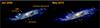 |
Fig. 1 Left: NGC 2770 observed with VLT (+FORS1) in January 2008, while there were two active SNe. An earlier SN from 1999 is indicated by a circle. Right: In May 2015 the SNe are gone in this image from GTC (+OSIRIS), but there is a new object, SN 2015bh, an LBV that potentially suffered a terminal explosion as a SN IIn. |
2.1. Imaging
Archival imaging data are available at irregular intervals since 1994 from the 1 m Jacobus Kapteyn Telescope (JKT), the 2.5 m Isaac Newton Telescope (INT) using the Prime Focus Cone Unit (PFCU) and the Wide Field Camera (WFC) and WHT. The LBV is detected in most of these observations except for a few epochs taken in poor conditions. Further data are available from SDSS taken in March 2004 in u′g′r′i′z′ bands. During the observations of SN 2008D from Jan. to March 2008 frequent imaging is available from ALFOSC at the Nordic Optical Telescope (NOT) in La Palma and FORS1+2 at the Very Large Telescope (VLT) on Chile. Further observations were used from the Hubble Space telescope (HST) archive for 5 epochs in 2008 and early 2009. Acquisition images in r′ from a drift-scan spectroscopy program at the Gran Telescopio Canarias (GTC) were obtained in Nov. 2013, serendipitously covering the onset of episode 2013A. Finally, we used images during episode 2015A from Asiago and from a UVOT/Swift programs (PI. P. Brown) in Feb. 2015.
On March 27 and April 9 2015 we observed NGC 2770 with OSIRIS/GTC using narrow continuum filters to complete a dataset on NGC 2770 during which we discovered that the source was still bright, and we decided to undertake a dedicated follow-up of the event. We then obtained weekly r-band observations through a DDT program (PI A. de Ugarte Postigo) at the Observatorio de Sierra Nevada (OSN) in Granada, Spain, using both the 1.5 m and the 0.9 m telescopes, with which we discovered the rebrightning on May 16, 2015, called the “main event” or episode 2015B. On May 9, we also obtained one epoch with the nIR imager Omega2000 at the 3.5 m telescope at Calar Alto Observatory (Spain) in J,H and KS bands.
Subsequently, we requested ToO observations by Swift/UVOT (PI S. Campana) with daily monitoring until the end of May 2015 and then at larger intervals until the object was too close to the Sun in mid June 2015. During the UVOT observations, XRT also observed the source in photon counting mode at 0.3–10 keV. Dense photometric monitoring of the main event was done from the ground with OSIRIS at the 10.4 m GTC (PI A. de Ugarte Postigo), the 0.5 m telescope at the University of Leicester, UK (UL50), the 0.6 m Rapid Eye Mount telescope (REM) at La Silla Observatory, Chile, and further observations with the OSN telescopes. Together, these observations provide us with an almost daily coverage of the LC from May 16 to June 20. NIR observations were performed at several epochs during episode 2015B with the REM telescope.
After the object became visible again by the end of September 2015 we continued the monitoring of the object until January 2016. Photometry in B,V, RI were obtained weekly using the 1.5 m OSN telescope, but the detection proved to be increasingly difficult, especially in the blue bands. On Nov. 26 we also obtained IR observations in J-band using the PAnoramic Near Infrared CAmera (PANIC) at the 2.2 m telescope in Calar Alto Observatory during its science verification phase. The observation consisted of 9 × 82 s under non optimal conditions and the object was detected at low S/N.
The optical and NIR images were reduced using IRAF with standard routines and pipelines developed for the different instruments or self-made procedures. After registering the images with alipy v2.0 and nshiftadd.cl they were coadded and astrometrised with astrometry.net2 (Lang et al. 2010). Aperture photometry was done for the different datasets using apertures of 1–1.5 × FWHM depending on the instrument and seeing conditions. Photometric calibrations were performed using SDSS for those images taken in Sloan filters, 2MASS for images in nIR and reference stars from Malesani et al. (2009) for images in John-Cousin filters. The result of all the photometric observations can be found in Table A.1. The light curve (LC) in R-band from 2008 to 2015 indicating the different episodes mentioned in the text is plotted in Fig. 2.
2.2. Spectroscopy
At the onset of episode 2013 (Episode 2013A) we serendipitously obtained spectra on 11 November 2013 with OSIRIS at the 10.4 m GTC during a drift-scan spectroscopy run to observe NGC 2770 and its satellite galaxy NGC 2770B. Episode 2013A was also detected by iPTF in December 2013 and spectra taken using GMOS-N, but the observations were first published in Ofek et al. (2016). Following the detection of the precursor in Feb. 2015 we performed spectroscopy on April 14, close to the maximum of the 2015A episode. Early data of this episode from February 2015 were published by the Asiago collaboration and included in our dataset.
Starting from the onset of episode 2015B/main event on May 16, we pursued an intense spectroscopic monitoring using primarily OSIRIS at the 10.4 m GTC and grism R1000B (3700–7800 Å), on a few occasions supplemented by grism R1000R (covering up to 10 000 Å). On June 4 and 6 we also obtained medium resolution observations from 5580 to 7680 Å using the R2500R grism. Further visible spectra were taken with TWIN and CAFOS at the 3.5 m and 2.2 m telescopes of the Calar Alto Observatory (Almería, Spain). High resolution spectra were obtained using HDS at Subaru (R ~ 40 000). We finally took three late epochs after the Sun gap in September 2015, November 2015 and January 2016 using OSIRIS/GTC and a single observation on Dec. 5, 2015 using FOCAS/Subaru. The log of observations is detailed in Table 1.
Spectra were reduced with standard procedures in IRAF and flux calibrated with standard stars taken the same night. The TWIN spectra show some issue in the flux calibration altering the shape of the spectrum, the reason for which is unknown and we hence exclude these data from any analysis requiring flux calibrated spectra. The Subaru data were reduced using the procedures described in Maeda et al. (2015) for the HDS data and Maeda et al. (2016) for the FOCAS data.
Log of the spectroscopic observations of SN 2015bh and its precusors.
2.3. Tuneable filters and driftscan spectroscopy
An ongoing project within our collaboration analyzes spatially resolved spectroscopic data of NGC 2770. Two of the datasets also cover the position of SN 2015bh: 1) Tuneable narrowband filter (TF) observations in [NII], Hα and [SII] were taken between 2013 and 2015 using the Fabry-Perot tunable filters at OSIRIS/GTC and cover all of NGC 2770. 2) A data cube obtained by drift-scan spectroscopy with the longslit spectrograph of OSIRIS/GTC in November 2013 at the onset of episode 2013A. The spectra cover the wavelength range from 3600 to 7900 Å at a spectral resolution of 2.6 Å and a spatial sampling of 1.2 arcsec, the data cube only covers the central part of NGC 2770.
The TF data contain Hα, [NII], the [SII] doublet and continuum observations, although [SII] is not used in this paper. To disentangle Hα and [NII] we used filter widths of 12 Å in steps of 8 Å. To improve the continuum subtraction and to obtain coverage in a blue filter we performed observations in three order separating filters (width 13–45 Å) roughly corresponding to g′, r′ and i′ filters in March 2015. The images were reduced with standard image reduction techniques. To account for the wavelength shift across the field, we assigned the true wavelength to each step in the scan using the wavelength dependency from the optical axis as described in Méndez-Abreu et al. (2011). Then we shifted the profile in each pixel to a common rest frame before integrating over a fixed wavelength range for each emission line. This shift was not applied to the continuum filters. No absolute flux calibration was done.
The driftscan data were reduced as 2D longslit spectra and wavelength calibrated. For each OB a template trace was extracted using a bright isolated region in the galaxy. We then extracted 50 regions per 2D spectrum, shifting the template trace by equal steps. The resulting 1D spectra were flux-calibrated using a single sensitivity function derived from a standard star observation during a photometric night and combined into a 3D data cube.
In both datasets the site of SN 2015bh is contaminated and/or dominated by emission from the LBV itself, either during a more quiescent state (part of the TF dataset, see Fig. A.1) or even during one of the pre-explosion outbursts (drift-scan dataset). Hence, we cannot use the data to measure any properties at the site of SN 2015bh directly, instead we can only infer properties from nearby SF regions. Here we use the part of the datasets described above in the vicinity of SN 2015bh. Including the full dataset is beyond the scope of this paper and will be presented in a separate paper (Thöne et al., in prep.)
 |
Fig. 2 Top: light curve of the progenitor of SN 2015bh from 1994 until 2016, the insets are blow-ups of episode 2008 in different colors and episodes 2015A&B (main event and precursor). SN 2009ip is also displayed for comparison and shows a very similar behavior. |
3. Evolution of the LBV 2008-2015
3.1. Photometric monitoring
Archival imaging dating back 21 yr before the main event indicate that the progenitor of SN 2015bh had been in an active state for at least two decades (see Fig. 2). Until the discovery in 2013 by iPTF and the detection of SNhunt275 in Feb. 2015, the LBV progenitor had falsely been identified as an Hii region in the same spiral arm of NGC 2770 as SN 2007uy, hence there are only serendipitous observations of the object during these years. We note that the position of the object inside a spiral arm of NGC 2770 might result in problems of crowding, especially using observations at low angular resolution, however, the progenitor of SN 2015bh seems to be fairly isolated and the underlying SF region, if any, seems to be very faint, hence we do not this this is an issue for our archival LC determination.
Already in 1994, the object was likely in a non-quiescent state with an absolute magnitude of –11 in V. Further single R-band detections in 1996, 2002 and 2004 ranging between –11 and –12 mag also indicate ongoing outbursts. During the dense observations in 2008 at the time of SN 2008D (see Fig. 2, inset a), significant variability was observed ranging between ~–9.8 mag and –12.1 in R-band: at the onset of SN 2008D on Jan. 10, 2008 and the subsequent ~30 days, the LBV was in a declining phase after a potential earlier outbust, fading to an absolute magnitude of ~–10 mag (episode 2008A). Another episode was observed around the turn of the year 2008/2009 (episode 2008B) with HST with a rebrightning of less than 2 mag and a quick subsequent decline. The color of the object usually turned redder during outbreaks after which it returned to a bluer state.
We also have archival radio observations of the object from the time of SN 2007uy and SN2008D as it was in the FoV of the Westerbork Synthesis Radio Telescope. Observations were performed on Jan 19 and 20, 2008, Nov. 15 and 16, 2008 and Sep. 12 2009 (van der Horst et al. 2011). The object was not detected in any of the epochs, which in fact were performed during an LBV outburst phase, with a limit of ~0.1 mJy or 8.7 × 1026 erg s-1 Hz-1 at 4.8 GHz (A. van der Horst, priv. comm.). SNe IIn have often been elusive in radio wavelengths, nevertheless some SNe with luminosities above our limits have been detected (see e.g. Margutti et al. 2014) albeit radio LCs are peaking at late time (>50 days post maximum).
During the following years, only narrow-band TF images of Hα and the continuum around the line were obtained which likely contain part of the asymmetric LBV Hα emission and are hence not reliable for inclusion in the light curve. A single observation from INT in Feb. 2012 showed the LBV at R = 19.8 mag (–12.6 mag) probably indicating another outburst phase.
In Nov. 2013 we serendipitously obtained images and a spectrum while observing NGC 2770B (a the satellite galaxy of NGC 2770) with driftscan spectroscopy covering also the central part of NGC 2770 and the site of SN 2015bh. By chance, we caught the object at the onset of another outburst (episode 2013A) with an increase in brightness from R = −10.2 to –12.5 mag. This outburst was detected later by iPTF, classified as an LBV outburst and named “iPTF13evf”. On Dec. 21, 2013 the object had faded to the level of comparison images taken between Jan. and Apr. 2014 Ofek et al. (2016). Those authors also searched the PTF and Catalina Real Time Survey (CRTS Drake et al. 2009) archives for other possible outbursts. No detections are made with PTF up to ~mag 21 (or –11.4 mag) up to 240 d before the 2013 episode and no outbursts brighter than magnitude 19 (or –13.4 mag) from CRTS until the precursor 2015A. Possibly no other major outburst happened at that time, although our detection from INT in 2012 would have been missed by those surveys.
3.2. Features in the spectra during the LBV phase
Our serendipitous spectra from the onset of episode 2013 are the only public spectra of SN 2015bh before the precursor event 2015A. Our full set of spectra from the episode 2015B throughout the main event is plotted in Fig. 3, in Fig. 4 we furthermore plot distinct epochs together with line identifications.
The spectrum from Nov. 2013 is characterized by intense narrow P Cygni profiles of the Balmer series, Fe II and Ca II, but no He I lines. The Balmer emission lines are very narrow (FWHM ~ 600 km s-1) and show a steep drop in the blue wing towards the absorption part of the P Cygni profile. This single, narrow P Cygni profile basically stays unchanged from 2013A throughout the main event and is probably reminiscent of material ejected prior to 2013.
The spectrum of that time looks similar to an LBV in quiescence or at least free of CSM interaction, which is not available for any other SN or impostor so far. We find a good match between the Nov. 2013 spectrum and a model for an LBV as described in Groh et al. (2014). The best-fit model from this work results in values of L = 1 × 10⁶L⊙, Teff = 8500 K, a mass loss rate of Ṁ = 5 × 10⁻⁴M⊙ yr-1 and a wind terminal speed of 600 km s-1 for SN 2015bh during the LBV phase (see Fig. A.1). This is similar to Eta Carinae today with the stellar radiation propagating through a dense wind. A full model of this stage will be discussed in a forthcoming paper (Groh et al., in prep.).
Ofek et al. (2016) published spectra taken with GMOS/ Gemini-N on Dec. 13, 2013, one month after our spectrum and during the maximum of the 2013A event. The spectra are of lower resolution, S/N and cover a smaller wavelength range. The only feature clearly detected is Hα and some weak tentative detections of various He I transitions also present in later spectra during the precursor in 2015. These authors measure the velocity of the absorption component of the P Cygni profile at –1300 km s-1 which is slightly higher than what we observe in the Nov. 12 spectra. The most curious feature is an absorption trough blue wards of Hα, which, if associated to Hα would have a velocity of ~–15 000 km s-1. However, it remains unclear whether this feature is real or due to some unknown reduction issue.
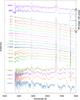 |
Fig. 3 Spectroscopic evolution of the LBV and SN, including two epochs during the LBV outbursts (episode 2013, –559 d and episode 2015A at –39 d) and a closely sampled time-series during the possible SN explosion from May 16 to June 19 (–7 to +27 d). After a gap in the observations due to sun constraints we obtained four new spectra in late September (+126 d), November 2015 (+181 d), December (+195.4 d) and January 2016 (+242 d). |
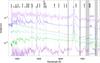 |
Fig. 4 Optical spectrum at 6 representative epochs and line identifications. Not all lines are visible in all epochs. The grey bars indicate atmospheric lines. Color coding of the spectra is the same as in Fig. 3 |
4. The 2015A event and possible SN explosion
4.1. Light curve evolution
There are no public data of SN 2015bh between the Dec. 2013 and Feb. 2015. The detection by SN hunt as “SNhunt 275” had an absolute magnitude of –13, slightly higher than during the last observed outburst in 2013. Spectra taken on Feb. 10 reported asymmetric Balmer lines and classified this event as a “SN impostor” (Elias-Rosa et al. 2015). We obtained our own imaging data in late March and early April 2015, showing a further increase in brightness. During our subsequent monitoring, the object rose to a maximum of R = −13.9 mag (around 25 days before the SN explosion), after which it declined to R = −13.6 mag on May 12, 2015. We call this episode the “precursor” or episode 2015A (see Fig. 2, inset b). Both the shape and magnitude difference of the precursor resemble the one observed for SN 2009ip.
On May 16, our weekly monitoring from the 1.5 m OSN telescope showed that the event suddenly brightened by ~2 mag, and continued to rise in the following days. The maximum R = 17.3 mag was reached around May 24 (which we define as T = 0 of the main event 2015B), after which the LC started a linear decline. The main event of 2009ip was slightly brighter but had similar rise and decay times. In addition, it showed a small “bump” during the decline post maximum not observed for SN 2015bh although it could have been missed by the observational gap between June and Sep. 2015. Both SN 2009ip and SN 2015bh were affected by observational gaps of ~3 months due to Sun constraints, so the exact evolution between ~30–120 days and 50–180 days for SN 2015bh and SN 2009ip, respectively, is not well determined. At late times (>100 d), the LCs of both events flatten and subsequently decay very slowly. As of June 2016, SN 2015bh remains in this shallow decline phase.
During the UVOT observations at the main event, we took simultaneous observations with XRT onboard Swift from May 16 to June 7, 2015 but fail to detect any X-ray emission at any epoch. Single observations of ~2 ks reach a limiting 0.3–10 keV unabsorbed flux of 3 × 10-13 erg cm-2 s-1 assuming a power law spectrum (with Γ = 2 and the Galactic column density of 2 × 1020 cm-2, Kalberla et al. 2005). At a distance of 27 Mpc this converts to an X-ray luminosity LX< 3 × 1040 erg s-1. Integrating the full set of X-ray observations we collected 48 ks and derive an upper limit of 5 × 10-14 erg cm-2 s-1 (LX< 4 × 1039 erg s-1). X-ray emission from SNe IIn have been detected with peak luminosities up to 3 × 1041 erg s-1 for SN 2010jl (Chandra et al. 2015). SN 2009ip showed some X-ray emission at peak with low significance at ~2.5 × 1039 erg s-1 and was detected at 9 GHz with ~5 × 1025 erg s-1 Hz-1 (Margutti et al. 2014).
After the object appeared behind the Sun again in late September 2015, the LC had dropped to ~–12.5 mag, a similar brightness to the object during the outbursts before the main event. In the following months until the end of our observing campaign in Jan. 2016, the light curve kept declining albeit with a very shallow slope.
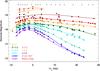 |
Fig. 5 Light curve in different bands during the main episode (2015B) and polynomial fits to the LCs. Grey arrows indicate the dates where we obtained spectroscopy. |
4.2. Spectral energy distribution, temperature and radius
During the main event, starting May 16, we have sufficient data to fit the SED from UVW1 (~1500 Å) to z/H-band (IR data are only available up to day 6 post maximum). We further have an early SED on May 9 during the pre-explosion event using J,H,K observations from Omega2000 and a late epoch on Nov. 27 (184 days post maximum) using the J-band observations from PANIC.
In Fig. 5 we show the multi band LC during the main event, in Fig. 6 we plot the complete SED evolution and a fit with a single expanding and cooling BB. The data are observed flux densities and the BB has been corrected for foreground extinction (AV = 0.062 from Schlafly & Finkbeiner 2011) as well as extinction in the host galaxy. The latter is determined via the resolved NaD doublet from the high-resolution spectrum on June 4. The NaD1 and D2 lines have EWs of 0.45 and 0.57 Å, respectively, applying the relation between NaD and extinction as described in Poznanski et al. (2012) we get an extinction of E(B−V) = 0.21 mag  . The high-resolution data from HDS/Subaru on May 30 give very similar values.
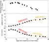 |
Fig. 6 Temperature and radius evolution of the BB fitted to the SED during the main event (see Fig. 7). In the top panel we plot the bolometric LC for comparison. |
During the first days, coincident with the rise in the LC, the BB gets hotter while the radius stays nearly constant (see Fig. 7). Past maximum, the radius increases with a rate of ~2300 km s-1 and about 15 days past maximum it slows down to 880 km s-1. In line with the radius, the temperature stays constant the first days, after which it cools with 660 K/day before slowing down to 150 K/day at 10 days post maximum. A similar change in the cooling and radius evolution was also seen in the last episode of SN 2009ip (Margutti et al. 2014), although the initial expansion velocity was slightly higher with ~4400 km s-1 but showed slower cooling rates (initially ~350 K day-1). Note also that the BB radius is significantly smaller than the one in SN 2009ip, although one has to be careful to associate the radius derived from the SED fit with a physical radius of the SN photosphere or interacting shell or when the radiating surface shows considerable asymmetry. The BB “radius” is therefore a lower limit on the “true” size of the radiating surface.
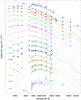 |
Fig. 7 SED from UV to IR from the precursor (one epoch), during the main explosion event until 180 days post maximum. The fit shown is a simple BB fit with varying temperatures. For the VIS bands we derive magnitudes using the flux calibrated spectra. In the last spectrum/SED, the R-band is clearly affected by the strong relative Hα line flux at that time. |
In the red and blue edges of the SED, a single BB does not seem to adequately fit the data (see Fig. 7). In the UV we observe two features: a drop in the UVM2 band past maximum of increasing strength, which likely originates from Fe II absorption lines at that wavelength (see e.g. Margutti et al. 2014). The excess in the UVW2 band is likely an instrumental feature: UVW1 and 2 have a leak in the red that becomes more pronounced for redder sources (Brown et al. 2010), and it in fact increases as the BB cools. In the IR we have a small excess in J and H band, starting already during the precursor but with no significant increase in strength. An additional component in the IR could be due to dust emission but should increase with time (see e.g. Gall et al. 2014). An IR excess has also been observed for 2009ip before maximum (Gall et al. 2012; Margutti et al. 2014) and attributed to emission from a shell expelled long before the main event. This explanation is also an appealing possibility for SN 2015bh. Unfortunately, we lack a good coverage in the IR to better assess an additional component due to pre-existing dust or dust production after the main event.
4.3. Bolometric LC and energy release
Using our photometry during episode 2015A and B we construct a pseudo-bolometric LC (see Fig. 8) following the method outlined in Cano et al. (2014): (1) we corrected all magnitudes for foreground and rest-frame extinction (see values in Sect. 4.2); (2) then we converted the AB UV/optical/NIR magnitudes into monochromatic fluxes using a flux zeropoint of 3.631 (×10-23 erg cm-2 s-1 Hz-1, e.g. Fukugita et al. 1995) to obtain flux densities (units of mJy). For epochs without contemporaneous observations we linearly interpolate the flux LCs to estimate the missing flux. Then, for each epoch of multi-band observations, and using the effective wavelength of each filter (Fukugita et al. 1995; Hewett et al. 2006; Poole et al. 2008) we (3) linearly interpolated between each datapoint; (4) integrated the SED over frequency, assuming zero flux at the integration limits, and finally (5) corrected for filter overlap. The linear interpolation and integration were performed using a program written in Pyxplot3.
During the precursor and the late epochs of the main event, there are not enough multi-band observations to determine the bolometric luminosity using the method described above. In order to construct a bolometric LC at those times we apply a different method by fitting the Planck function to each epoch of multi-band photometry to determine the black-body temperature and the radius of the blackbody emitter. Then, we integrated the fitted Planck function between the filter limits of our data (UV to I-band) in order to consider the same frequency range as that used when constructing the filter-integrated bolometric LC. The fitting and integration were performing using custom python programs. Both the shape and peak luminosity of the two bolometric LCs agree very well.
From the bolometric LC we derive estimates of the total energy release during the different events: The 2015A event released 1.8 × 1047 erg, though we must consider the caveat that this estimate only includes data obtained over three epochs, i.e. days –145 to –45. The first epoch of observations of the main event until the object disappeared behind the Sun counts with a total release of 1.2 × 1049 erg. Adding the luminosity of the observations after the object became visible again does not significantly increase the total energy release (the total energy between day 121 and 242 is 9.9 × 1046 erg). Assuming a linear interpolation during the time when the object was not observable yields a total energy release of the main event (2015B) of 1.8 × 1049 erg. Ofek et al. (2016) estimated a total energy release of >2.4 × 1046 erg for the LBV outburst in 2013.
4.4. Spectral evolution and line profiles
We modeled the different components in Hα and Hβ in our complete set of spectra. In Figs. 9 and 10 we plot the Hα and Hβ profiles at different representative epochs and the changes of the absorption and emission components over time.
The spectra of the precursor largely resemble those of the onset of the LBV outburst in 2013. While the P Cygni profile during the LBV phase only showed one absorption component, an additional a weak second absorption component in the spectra of the precursor maximum in April 2015. This could be the onset of the double absorption profile appearing post maximum of the main event and would imply that this faster material (v ~ 2000 km s-1) is directly related to the precursor (2015A) event, a possibility also noted by Ofek et al. (2016).
From the onset of the main event up to maximum the line profiles become rather smooth and almost symmetric with broad wings and very little (visible) absorption, although still present. HeI emission lines appear and get more pronounced while the Fe II lines disappear. This could be due to flash ionization of the material and time dependent recombination, affecting different transitions at a different timescale. The velocity of the narrow absorption component (and to a smaller degree the emission component) slightly decreases until maximum light although only by ~150–200 km s-1. There could be a similar tendency in the faster absorption component but fitting around maximum is difficult and has large errors. The FWHM of the broad absorption component decreases past maximum while the one of the narrow component slightly increases. These effects are probably associated to the increase in radiation field around maximum, ionizing the inner part of the emitting and absorbing shells.
In this phase, we also observe some broad “bump” blue wards of Hβ. It is not clear whether this bump is also present blue wards of Hα. If associated to the Balmer lines, this would mean some material ejected at very high velocities (~13 000 km s-1) Alternatively it could be a blend of NIII λλ 4634, 4640, C III λ 4647, 4650 and He II λ4686 as was also observed in the Ibn SNe 2013cu (Gal-Yam et al. 2014) and 2015U (Shivvers et al. 2016) and the type IIn SN 1998S (Shivvers et al. 2015). At +26 d and beyond there is some conspicuous bump in absorption blue wards of Hβ and possibly Hα, albeit at somewhat lower velocities (~7000 km s-1).
Past maximum, the spectrum starts to show clearly the double absorption profile with an increasing strength in absorption in time. It is important to note that the double absorption system is visible in all line, implying that the first and second shell corresponding to the two components have very similar abundance patterns.
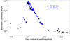 |
Fig. 8 Bolometric LC of the precursor (episode 2015A) and the main explosion event of SN 2015bh (epoch 2015B). As comparison we also plot the bolometric LC of SN 2009ip obtained in the same way as for 2015bh. |
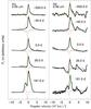 |
Fig. 9 Components fitted to the Hα and Hβ line at different representative epochs. The colors of the components are identical to the ones in Fig. 10: red/orange are the narrow P Cygni profile emission and absorption components, blue/turquoise the broad components and green the total fitted profile. |
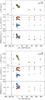 |
Fig. 10 Properties of Hα and Hβ derived from the component fits during the LBV phase, precursor and the main event. From top to bottom: total luminosity, velocity shift and FWHM and flux of the different components. Round symbols correspond to absorption components, triangles to emission components. Colors correspond to the components fitted as shown in Fig. 9. |
After the Sun gap at >126 d, the spectra had changed dramatically with FWHMa of several thousand km s-1. Hα has double peaked profile that can be modeled with the original emission component at the same velocity and an additional component at ~–2000 km s-1, the same velocity as the second absorption component observed before the observational gap. This could be an indication that those two components are related (see Sect. 4.7).
HeI λ5889 and λ7065, which had disappeared in late June, show up as broad emission lines with the same broad profile as the Balmer lines. A strong [CaII] λλ7291, 7323 doublet is also visible in those spectra. Fe II becomes visible again in emission, but shows a smaller FWHM than the other emission lines. The spectra thus resemble that of a nebular SN, with the exception that there are still absorption components present. A possible interpretation is that the ejecta have become optically thin and we are now seeing deeper into the material with a wide range of velocities.
4.5. Hα equivalent width
The Hα EW shows some remarkable changes throughout all phases (see Fig. 11). During the outbursts and the precursor, it had an EW of around 200 Å, during the main event it dropped to values of 50 Å after which it rose again to finally of values of more than 1000 Å at >126 days.
A similar behavior has been observed for other IIn SNe and also SN 2009ip (Smith et al. 2014). The EW evolution is very similar to the one of SN 1998S, a genuine type IIn SN. SN 2009ip had values of close to 1000 Å during the pre-explosion outbursts years before the main event, and increased again to even somewhat higher levels after the main event. Smith et al. (2014) interpret the large increase in EW as evidence for a terminal explosion of SN 2009ip as this takes place when the interacting material from the SN becomes optically thin, causing the continuum to drop and the Hα photons from the shock escape more easily.
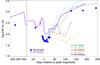 |
Fig. 11 Hα EW evolution from the LBV phase to the possible SN explosion. For comparison we also show the EW evolution for SN 2009ip and several there type IIn SNe (data from Smith et al. 2014, and F. Taddia, priv. comm.) |
4.6. Evolution of the Balmer decrement
Another interesting aspect is the evolution of the Balmer decrement Hα/Hβ (see Fig. 12), which in Case B recombination has a value of 2.73 in absence of extinction. While it showed relatively high values during the outburst and precursor (8.5 and 3.5), it dropped to values below Case B recombination around maximum. From ~day 10 on it rises again reaching up to values of 6–10 at late times, depending on the method used (i.e. taking the ratio of the peak fluxes or the ratio of the line fluxes).
SN 2009ip showed a relatively normal Balmer decrement of 3 ± 0.2 during the precursor but then dropped to a value of 1.1–1.3 during the peak of the main event (Levesque et al. 2014). The authors explain this with a very dense (ne> 1013 cm-3) plasma in the ejecta which thermalizes the emission due to collisions. At late times of ~200 days, however, the Balmer decrement of SN 2009ip increases to a value of 12 (Fraser et al. 2015). This is typical for nebular phases of outbursts from different objects when they cool and become optically thin and is caused by hydrogen self-absorption. Similar high Balmer decrement values have been observed in a number of other objects such as expanding shells of novae (Iijima & Esenoglu 2003) and the outflow from an X-ray binary outburst at late times (Muñoz-Darias et al. 2016).
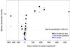 |
Fig. 12 Balmer decrement evolution using total integrated and peak fluxes of Hα and Hβ and comparison with SN 2009ip (data from Levesque et al. 2014, who uses peak flux values, and Fraser et al. 2015). |
4.7. A possible geometry of the event
From the evolution of the spectral lines we can get some idea on the geometry of the event (see Fig. 13). We caution that this geometry is simplified to be symmetric while the line profiles actually show indications for some small degree of asymmetry. The narrow P Cygni profiles had remained rather constant since the LBV outburst in November 2013. This implies that the material must have been so far from the star that it remained fairly unaffected even during the main event. We associate this to a thin shell at a large distance from the star moving with a moderate speed of v ~ −700 km s-1 that was expelled many years back in the past as also suggested by Ofek et al. (2016). Another possibility is that this component comes from a stellar wind sweeping up the CSM.
The second broad absorption component with v ~ −2000 km s-1 that already appears during the precursor becomes more pronounced after maximum. At >126 d this absorption component is replaced by a second component in emission at the same velocity. A possible scenario is that this second component is associated with a shell expelled at the time of the precursor that finally catches up with the v ~ −700 km s-1 shell and shock excitation leads to an emission component at –2000 km s-1. Assuming that the second shell was expelled around –50 d, at ~100 d, when the fast emission component appears, the shell would have reached a distance of ~2.5 × 1015 cm, which is at the same order of magnitude as the extrapolation of the BB radius evolution (see Fig. 6) out to 100 d. Alternatively, the material becomes optically thin, with the material that had first shown up in absorption now appearing as emission component.
SN 2009ip is thought to have a complicated geometry: Based on polarization measurements Mauerhan et al. (2014) propose a toroidal CSM with which the ejecta interact. The main event itself is also asymmetric but orthogonal to the toroidal CSM implying a bipolar shape of the SN photosphere or ejected shell at the main event. A similar conclusion was reached by Levesque et al. (2014) who propose a disk-like geometry of the ejecta to explain the observed (low) Balmer decrement around maximum which would require very special conditions in a shell-like structure. SN 2015bh has a similar behavior of the Balmer decrement with values below 2.73 during maximum albeit less extreme than SN 2009ip.
We also note the presence of a small additional emission component in the red wing of Hα at late times with a velocity shift of ~+2000 km s-1 which would be the receding counterpart of the second emission component showing up in the late time spectra. A curious case is SN 1998S which showed a triple-peaked Hα profile at late times, which could imply a similar scenario but very asymmetric or bipolar ejecta or a different viewing angle.
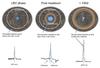 |
Fig. 13 Sketch of the event during the LBV phase, after maximum brightness and at late times (>120 d) together with the corresponding profiles of Hα. The LBV is embedded in a dense CSM indicated by the grey shaded area. During the LBV phase, only one absorption component is present while post maximum, after the emission starts to fade, a second component becomes visible in all emission lines which we therefore attribute to a shocked region associated to the shell ejection or SN explosion. At late times, the second component shows up in emission, either implying that the second shell has interacted with CSM (probably the earlier ejected shell) or that is has become optically thin. |
4.8. Modeling of the main event
We provide an order-or-magnitude estimate on the physical quantities related to the main event 2015B using the bolometric LC and other observational constraints. First, we fit the bolometric LC within the context of the “shell-diffusion” model (e.g. Arnett 1982, 1996; Smith & McCray 2007) as shown in Fig. 14. This model assumes that the ejecta crash into the dense CSM creating an optically thick, dense shell. This shell then cools down through adiabatic losses while the optical emission is created through diffusion. For the model in this figure, the parameters are M0 ~ 0.5 M⊙ (the mass of the dense shell including the swept-up ejecta) and R0 ~ 5 × 1014 cm (the initial distance to the shell). The LC decline is well reproduced by the diffusion model which supports the main physical assumption of the model. These are comparable to those obtained for SN 2009ip through similar analyses (Margutti et al. 2014; Fraser et al. 2015; Moriya 2015).
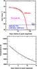 |
Fig. 14 Model fit to the bolometric LC and temperature evolution. |
The physical parameters are further constrained by the temperature evolution assuming a BB emission. Figure 14 shows the temporal evolution of the photospheric temperature based on the diffusion model, as compared to the one obtained from the BB fit to the SED. In this particular model, the parameters are M0 = 0.005 M⊙ and R0 = 4.5 × 1014 cm, and v = 2300 km s-1, where v is the velocity of the shell after the crash. The values are different from those obtained through the bolometric LC model, however, we caution that our model is very simplified. Therefore, our conservative estimates are M0 ~ 0.005−0.5 M⊙ (therefore E ~ 1047−1049 erg with v = 2300 km s-1) and R0 ~ 5 × 1014 cm. The distance to the shell is fairly consistent with the idea that it was created by the pre-explosion event 2015A about two months before.
The predicted LC as powered by the interaction with the CSM shell created at the 2015A event drops after ~30 days, after this the possible power source is the interaction with the CSM created before the 2015A event (likely by the 2013A event). Interestingly, the late-time luminosity is nearly constant after ~100 days. This suggests that the expanding dense shell is not decelerated any more (see also Moriya 2015). Adopting 2300 km s-1 as the constant shell velocity (i.e., free-expansion) expanding into the outer part of the CSM which was created before the 2015A event, the CSM density to explain the luminosity in this late phase corresponds to the mass loss rate or ~0.008 M⊙ swept up in ~30–100 days. The need for free expansion is then rephrased that this swept up mass should be smaller than M0, i.e., M0 > 0.008 M⊙, which is indeed satisfied (see above).
The 56Ni mass potentially produced in the 2015A event must be <0.005 M⊙, otherwise the predicted luminosity would exceed the luminosity in the late-phase (Fig. 14). Even including the uncertainty in the explosion date conservatively as large as 100 days, the upper limit would be ~0.01 M⊙. The small amount of 56Ni also agrees with our energy estimate, ~ 1047−1049 erg, which is not large enough to lead to explosive nucleosynthesis of 56Ni. In sum, the physical quantities we derived are all much smaller than those for typical CC SNe. This could mean that we actually do not have a CC event here.
5. The progenitor star and its evolution
Obtaining information about the progenitor star is hampered by the fact that the LBV has been in outburst as far back as 1994. The two epochs with the lowest luminosities during the 21 yr of observations were in early February 2008 and a year later in January/February 2009: at both times it had an absolute magnitude of ~–8 in R-band. Whether these epochs correspond to a genuinely “quiescent” state is debatable, in fact, it is more likely that the LBV was in a hot phase of the S Dor variability cycle or another type of outburst state in these epochs.
In Fig. 15 we plot the evolution of the object throughout the different states of outbursts (“LBV phase”), the precursor, the main 2015B event, and the subsequent post-maximum decline. We take the luminosity in R-band while the temperature is derived from V−I colors. We also plot stellar evolution tracks from the Geneva models (Ekström et al. 2012) for progenitors of 20–60 M⊙ at solar metallicity (although the true metallicity is closer to half solar, see Sect. 6) and with zero rotation. Furthermore we obtain data from the literature on Eta Carinae (Rest et al. 2012) and SN 2009ip (Pastorello et al. 2013; Fraser et al. 2015).
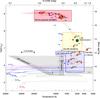 |
Fig. 15 HR diagram showing the evolution of SN 2015bh during the early outbursts, throughout the precursor, main event and decline (red dots). The boxes indicate the region in which SN 2015bh was located during different phases of the evolution. Blue dots show the same for SN 2009ip from 2009 to 2015 (data from Pastorello et al. 2013; Fraser et al. 2015). The last observation at –9.1 mag (R-band) is below the proposed progenitor level from HST observations in 1999 (blue dotted line, no color information is available for this epoch). We also plot data for Eta Carinae (Rest et al. 2012) today and during the main eruption as well as the range of LBVs between quiescence and outburst. |
5.1. Evolution through the HR diagram
Since 2004, the LBV was redder than S-Dor like LBVs during outburst, even during the periods of lowest luminosity: such states can be considered (perhaps falsely) as quiescent. LBVs typically have much higher temperatures during quiescence and become (visibly) cooler during outburst when the outburst shell detaches from the stellar surface, while remaining nearly constant in bolometric luminosity. Our object never reaches the temperatures of LBVs in quiescent state, and instead are similar to Eta Carinae during its giant eruption in the 1800s, albeit at a lower luminosity.
A possible interpretation is that the outbursts observed from 1994 to 2015 are a type of Eta-Car like giant eruption followed by a much more violent outburst or SN that Eta Car has not experienced (yet). The difference in luminosity might simply be a consequence of the higher mass of Eta Car compared to the LBV progenitor of SN 2015bh. However, Eta Car-like eruptions usually last much longer, sometimes several years. Another possibility is that some of the observations, e.g. in April 2008, actually do correspond to the quiescent state of the star. In this case, the object would be a cool, yellow hyper giant (YHG) such as ρ Cas which are probably evolved red giant stars. YHGs also show variations in luminosity and occasionally suffer larger eruptions, e.g. every ~50 yr for ρ Cas; those objects are enshrouded by dust and material from their frequent eruptions. YHGs have been classified by the “Keenan-Smolinski” criterion which requires one or several broad components in Hα and broad absorption lines. In 2013, SN 2015bh showed emission lines with narrow P Cygni profiles which is a characteristic of LBVs in outburst. However, YHGs and LBVs can not always be clearly distinguished based purely on their spectra.
After the main event the object returned to the same luminosity as it had during the LBV outbursts, but showing lower temperatures. The emission at 240 days is likely still associated to the radiating shell from the shock interaction and not from the photosphere of the star (in case it is still alive). From its current position in the HR diagram the object can either return to a bluer and fainter state (as is the case for SN 2009ip, see below) or simply continue cooling and dropping out of the HR diagram as predicted for a terminal explosion. Future observations in a few years from now might be able to make a more concrete statement on the final fate of the star.
5.2. The possible progenitor star
The progenitor properties depend on whether the low luminosity periods actually correspond to a quiescent state or not. If the star was a yellow hyper giant (YHG) in quiescence, stellar evolution tracks indicate a very massive star of ~50 M⊙. In case the star has always been in a type of outburst, the true quiescent state of the star should be lower and hence its mass though how much lower is difficult to estimate. Considering the spectra during outburst resemble those of LBVs rather than YHGs, the progenitor in (unobserved) quiescence may be bluer and possibly fainter, though this is only speculation. Elias-Rosa et al. (2016) also note an erratic and fast-changing behavior of the possible progenitor from HST imaging, speaking against a “quiescent” state at any time in 2008–2009. The progenitor of the Type IIb SN 2013cu in fact was proposed to be a possible YHG but with lower wind velocities than SN 2015bh (Groh 2014). Another case could be SN 1998S (see a recent paper by Shivvers et al. 2015) whose spectra shows a lot of similarities with SN 2015bh and where indications for pre-explosion mass losses have been found.
Only a few SN IIn progenitors have been identified to date: SN 2005gl was proposed to be an LBV of >50 M⊙ (Gal-Yam et al. Gal-Yam et al. 2007) and disappeared in post-explosion HST images (Gal-Yam & Leonard 2009). SN 2010jl, a very luminous SN IIn, had a >30 M⊙ progenitor (Smith et al. 2011a). An LBV progenitor was also suggested for the ultra luminous SN IIn SN 1978K (Smith et al. 2007a) although no pre-explosion imaging is available. The progenitor of SN 2009ip is poorly constrained as pre-imaging was only obtained in one filter in 1999 and is consistent with a star of at least 60 M⊙ (Foley et al. 2011; Smith et al. 2014). Indirect evidence for mass-loss episodes such as complex absorption line profiles (e.g. Trundle et al. 2008) indicate the possibility of LBVs as progenitor stars. SNe IIn show a large variety in explosion properties (Taddia et al. 2013) and might come from a range of progenitors. This might be even more true for SN impostors of which some are related to LBV stars (see e.g. UGC 2773 OT 2009-1, SN 2002 kg, SN 2000ch and SN 1961V Foley et al. 2011; Van Dyk et al. 2006; Wagner et al. 2004; Goodrich et al. 1989; Kochanek et al. 2011) while others are from cool, red, “extreme AGB” stars of relatively low masses (~9 M⊙; Kochanek 2011).
5.3. Late-time evolution of SN 2009ip
SN 2009ip has been observed now for more than 3 yr since the main event in 2012 (Fraser et al. 2015), which allows us to study the possible future evolution of SN 2015bh which is nearly 3 yr “behind” 2009ip. During the outburst phase, precusor and main event SN 2009ip occupied a very similar region as SN 2015bh did from 1994–2014 (see Fig. 15), although SN 2015bh might have been slightly bluer during the main event (data taken from Pastorello et al. 2013). After the main event, SN 2009ip went back to the region of the precursor and, after a short turn towards cooler temperatures, now turned hotter and bluer again (data taken from Fraser et al. 2015). In 2014 it was only ~0.1 mag brighter than in the HST pre-explosion images.
To investigate its further evolution we took images on Nov. 30, 2015 we also obtained observations in g′,r′,′i′ with OSIRIS/GTC of SN 2009ip (Thöne et al. 2015), which revealed that the object has dropped below the level in the HST images in 1999 (Foley et al. 2011; Smith et al. 2014) and has become even bluer (see Fig. 15). Several authors (e.g. Graham et al. 2014; Margutti et al. 2014) already noted this blue-turn but argue that a BB fit might not be appropriate at this stage. We also caution that the HST data have been taken in the F606W filter that contains Hα, while we determine the luminosity from g-band data that does not contain strong emission lines, hence the star might actually be still close to its level form 1999 and not already significantly below it. The new observations imply that either the progenitor observed in 1999 was already in an outburst state and is now returning to its quiescent level or that it shed a lot of mass and its new quiescent state is lower or that 2009ip. Another possibility is that 2009ip is part of a binary system of which one exploded and we now only observe the companion.
We also obtained spectra of SN 2009ip on Dec. 23 using LDSS3C on the 6.5 m Magellan-Clay telescope (Las Campanas Observatory, Chile, see Fig. A.2). The spectrum shows little continuum and a huge, nearly symmetric Hα line with an EW of >3000 Å well as weak emission lines of Feii and NaD possibly blended with He I. Hβ is only marginally detected implying a Balmer decrement of ≳50. In comparison to spectra of SN 2009ip from May 6, 2014 (part of the PESSTO data release), the hydrogen lines except Hα have basically vanished while the Fe II emission lines are still visible. The late time spectra also seem different from “typical” SN IIn such as SN 1998S (Mauerhan & Smith 2012) or SN 2010jl (Fransson et al. 2014; Gall et al. 2014) which show the characteristic, broad nebular emission lines. This could imply that the dense ejecta visible at late times are actually not present here. If the progenitor of SN 2009ip survived those events as a kind of “zombie” star, it would reach its current end-state in only a few more years from now. Deep high-resolution imaging might settle the question about the nature of SN 2009ip soon. The spectra indicate that there is furthermore very little emission left from the CSM interaction at this stage, facilitating those observations.
6. The progenitor environment
Studying Hα maps of SN hosts, Anderson et al. (2012) argued that SNe IIn were less associated with HII regions than what would be expected if they (all) originated from very massive stars, and that they are even less associated with SF regions than the low-mass progenitors of SN type II-P. Smith & Tombleson (2015) found that LBV stars are usually isolated from star formation, which lead them to propose that they are mass gainers in binary systems rather than very massive stars. Taddia et al. (2015) studied the environments of 60 interacting SNe including SNe IIn, Ibn and SN impostors, and found that SN impostors and long lasting (SN 1988Z-like) SNe IIn are typically found at lower metallicities than SN 1998S-like IIns. They proposed that the former class originates from LBV progenitors, while the latter result from the explosion of Red Supergiants (RSG) in a CSM. Habergham et al. (2014) finally concluded that SNIIn and impostors are not associated to ongoing SF traced by Hα emission. Furthermore they conclude that “SN 2008S-like” impostors (those with low mass progenitors) fall on regions without Hα emission while “Eta-Car like” impostors (possible LBV progenitors) do have underlying Hα emission.
Our Hα tunable filter map of NGC 2770 indicates that SN 2015bh is probably not lying within a bright SF region. It is, however, in the same spiral arm as SN 2007uy in a row of smaller SF regions spanning from the region of SN 2007uy along the spiral arm. A definite answer as to whether it is associated to a SF region or not is hard to give since any image available of NGC 2770 is contaminated by the LBV and there might well be a faint underlying SF region. However, in contrast to SN 2009ip, it is clearly hosted within the galaxy in one of the star-forming outer spiral arms.
A map of the region around the LBV site corresponding to half of the data cube constructed from the drift-scan spectroscopy dataset (~5 × 2.5 kpc) is shown in Fig. 16. Since we cannot determine properties of the environment at the actual location of SN 2015bh (in all available spectra we have contamination from the LBV star), we study the properties at the SF regions in the same spiral arm SE and NW of the LBV location. The metallicity is derived from the N2 parameter in the calibration of Marino et al. (2013), the SSFR is obtained from scaling the Hα luminosity with the magnitude in the region of 3980–4920 Å of the spectrum, corresponding to the coverage of a B-band filter.
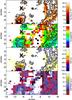 |
Fig. 16 The galactic environment of SN 2015bh in Hα, metallicity, Hα EW and specific SFR as observed with OSIRIS/GTC and drift-scan spectroscopy. The area covers about 5 × 2.5 kpc. Contours are from the TF observations of the Hα line. Note that the properties at the explosion site (marked by a cross) cannot be considered as the data are contaminated by emission from the LBV during outburst. |
The HII region to the SE is part of a cluster of several HII regions in one of which SN 2007uy was located (which is just outside the range covered by the driftscan cube). The SE and NW SF region have both a metallicity of 12 + log(O/H)= 8.46, Hα EWs of ~–40 and –10 Å and a specific SFR (SSFR) of ~3.1 and 2.1 M⊙/y/L/L*. The metallicity of both neighboring SF regions is below the mean of the metallicity gradient in NGC 2770 by about 0.06 dex and similarly low as for SN 2007uy and SN 1999eh (Thöne et al. 2009, and in prep.). Compared to other SN IIn site metallicities, SN 2015bh lies at the mean of the distribution (Taddia et al. 2015). The EW is rather low which would imply an age of the SF region of more than 7 and 10 Myr or the lifetime of a 25 or 17 M⊙ star for the two regions respectively. In line with this, the SSFR at both sites is rather low both within the galaxy and lower than any of the SN Ib sites (Thöne et al., in prep.). The fact that, in particular the region NW of the LBV site is neither very young nor particularly star-forming is supported by the absence of Hβ in emission, which is the case in many HII regions within NGC 2770, the HII cluster around SN 2007uy, however does show Hβ in emission.
7. Comparison with SN impostors and SN type IIn
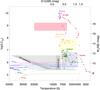 |
Fig. 17 Evolution throughout the HR diagram for several other events: The SN impostors SN 2008S, SN 2000ch and SNhunt248 and the type IIn SNe 1998S and 2010jl. Colored boxes correspond to the three main epochs of SN 2015bh as in Fig. 15. SN 2000ch occupies a very similar region to SN 2009ip and SN 2015bh in the LBV phase and could be a similar star in this pre-main event period. SN 2008S was always redder than SN 2009ip and SN 2015bh at much lower luminosities. SN 2010jl and SN 1998S reached higher magnitudes than the main events for SN 2009ip and SN 2015bh. SNhunt248 occupies a similar region during the outburst phase but has a lower luminosity at peak. The small late blue turn corresponds to a bump in the LC past maximum. |
7.1. SN 2015bh and SN type IIn
SNe IIn apparently span a large range of luminosities from SLSNe down to sub-luminous events which are difficult to disentangle from SN impostors. SN 2006gy (Smith et al. 2007b) and SN 2010jl (Stoll et al. 2011) with peak magnitudes of –22 mag and –20.5 mag, respectively, were classified as a SN IIn but had a much higher luminosity than typical SNe IIn (2006gy is now considered as the first SLSN-Type II detected). Most SN IIn show indications for massive progenitors, hence it might be a question of mass-loss through winds, eruptions and the structure of the CSM which defines the luminosity of the final explosion. Interacting SNe furthermore comprise H-poor events (SN Ibn) and even thermonuclear explosions (SN Ian).
Several classes of Type IIn SNe have been established in the past: SN 1994W, 1998S, 1988Z-like and “generic” SNe IIn (see e.g. Taddia et al. 2013; Kiewe et al. 2012). 1994W-like IIn (other members are e.g. SN 2009kn, Kankare et al. 2012 and SN 2006bo, Taddia et al. 2013) have a characteristic plateau post maximum (hence called SN IIPn), which is not the case for SN 2015bh. They have, however, a similar set of emission lines as we observe for SN 2015bh, but they never show the dramatic change to broad late-time emission lines. SN 1998S and 2008fq (Taddia et al. 2013) showed broad line profiles at >50 d and the Balmer line profiles actually resemble very much those of SN 2009ip. SN 1988Z-like SN such as SN 2006jd and SN 2006qq (Taddia et al. 2013) have very asymmetric emission lines with a broad component that can even be detached from the narrow component, and a suppression in the red wing due to dust (see e.g. SN 2010jl, Gall et al. 2014), which we do not observe here. Spectra of some type IIn SNe are shown in Fig. 18.
Precursors directly prior to the main event seem to be common in Type IIn SNe. Pastorello et al. (2007) was the first to report on a massive eruption that preceded the explosion of Type Ibn SN 2006jc that had been recorded in images obtained by amateur astronomers. Other well-studied examples are SN 2010mc (Ofek et al. 2013) and LSQ13zm (Tartaglia et al. 2016). Ofek et al. (2014) estimated that at least 50% of SNe IIn experience a major outburst in the last 100 days prior to explosion based on the pre-explosion observations of 16 SNe IIn detected by PTF. Precursor explosions have also been identified in the case of superluminous SNe (Leloudas et al. 2012; Nicholl et al. 2015; Nicholl & Smartt 2016; Smith et al. 2016a) although it is debated whether SLSNe are (only) powered by circumstellar interaction.
Outbursts years prior to explosion have only been detected in a few cases and comprise mostly single detections and no spectroscopy. Examples are SN 2011ht (Fraser et al. 2013b), SN 2006jc (Foley et al. 2007), a SN Ibn and PTF12cxj (Ofek et al. 2014). Ofek et al. (2014) argue that since outbursts and precursors are so common in type IIn, they should be directly related to the end state of very massive stars. The physical mechanism of these outbursts is still unknown and some argue that the “pre-cursor” is the actual explosion event while the brighter “main” event is caused by the interaction of the SN shell with the CSM.
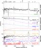 |
Fig. 18 Comparison between the spectra of SN 2015bh (black), SN 2009ip (blue), SN 1998S (a genuine type IIn), SN 2008S (an impostor) and SN at different epochs. Unfortunately, there are no spectra publicly available on SN 2009ip during the outburst phase, the same applies to the very similar event SNhunt 248 (Kankare et al. 2015; Mauerhan et al. 2015). |
7.2. SN 2015bh and SN impostors
SN impostors are classified as having peak luminosities of >–16 mag (Smith et al. 2011b) but else are a very diverse class. Rather than their peak luminosity, the LC shapes and outburst duration suggest different types of events within the SN impostor class. Several authors have tried to put SN impostors into different sub-classes based on various properties (see e.g. Smith et al. 2011b; Kochanek et al. 2012; Habergham et al. 2014), but the nature of those transients remains unclear. As a rough distinction we can divide SN impostors into three classes:
Large outbursts. This class of impostors has light curves with peaks of only a few magnitudes above the “quiescent” state. The outbursts can last several years and show a rather erratic behavior, the prototype of which are the eruptions of Eta Carinae in 1843 and 1890. The spectra have narrow emission lines similar to SNe IIn but usually without high velocity components or strong absorption components. Members of this class are SN 2002 kg/V37 in NGC 2403 (Weis & Bomans 2005), an LBV outburst, and U2773-OT (Smith et al. 2016b), a possible Eta Car giant eruption analogue. HD 5980 in the SMC is another interesting event, however, this system likely is a binary consisting of an LBV and a Wolf-Rayet (WR) star, the latter of which is variable and changed to a B-supergiant during outburst (Koenigsberger et al. 2010). In all of these cases, a star is clearly present after the outburst and hence those are genuine impostors.
Short-term outbursts. This class comprises shorter eruptions (timescale of a few weeks) that are longer than micro variations of massive stars (<0.5 mag). Their spectra are similar to LBV outbursts described above. In this class are SN 2000ch (Wagner et al. 2004) (and its subsequent outbursts in 2008–2009, Pastorello et al. 2010) and the pre-explosion outbursts of SN 1964V, SN 2009ip, SNhunt 248 and SN 2015bh. All of those short outbursts lead to a CC type IIn SN or a hyper-eruption except for SN 2000ch, which we will describe further below (Sect. 7.3). Many of these outbursts might be missed due to their faintness and the low cadence of current surveys.
Impostors with SN-type LCs. This class is the most difficult to distinguish from CC SNe IIn and some of them might actually be real CC events. Their LCs resemble “genuine” SNe with fast rises and slow decays that are either linear or have an early plateau similar to type IIP SNe. Their peak luminosities are lower than for typical type IIn SNe although there is a continuum of peak luminosities. The spectra of those events often look similar to type IIn SNe, some even showing high velocity components indicative of outflows more typical of SNe, hence a distinction based on the spectra is often hard to make. The definite classification of a SN impostor is a surviving star, but even this is still disputed for many SN impostors.
There are numerous examples in this class and probably a range of progenitors. SN 2008S-like impostors (which includes SN 2008S, NGC 300-OT and maybe SN 2010dn, Smith et al. 2011b) have relatively faint and red progenitors (Kochanek 2011) and occupy a very different region in the HR diagram (see Fig. 17). However, recent observations (Adams et al. 2016) reveal that those two objects are now fainter than the progenitor level in the IR. If they were indeed SN impostors, the surviving star has to be enshrouded by significant amounts of dust corresponding to >1 M⊙ of ejected mass, which seems unlikely for a <14 M⊙ progenitor. Other impostors such as SN 1997bs (Van Dyk et al. 2000), SN 2002bu (Szczygieł et al. 2012) and SN 2007sv (Tartaglia et al. 2015) could have either an LBV or a red giant progenitor but also here the final fate of the star is sometimes disputed (see e.g. the discussion on SN 1997bs Van Dyk et al. 2000; Li et al. 2002). There are many more events in this class but not always with very good observational coverage (for further examples see e.g. Smith et al. 2011b).
Finally, events with peak luminosities at the high end of impostors or low end of IIn SNe are highly disputed concerning their final state. The prototype of those is SN 1961V whose fate is still highly discussed (Kochanek et al. 2011; Van Dyk & Matheson 2012). More recently, SNhunt 248 (Kankare et al. 2015) seemed to show a very similar behavior but at lower peak luminosity. SN 2009ip and SN 2015bh would also be members of this class if we consider them impostors. All of these events have shown precursors which might either be an intrinsic property or simply an observational bias as corresponding precursors of the fainter SN-like class are very likely to be missed.
7.3. A new class of event?
The events described in the last paragraph suggest a new class of objects that either do or do not experience a core-collapse, but that nevertheless share a number of common properties: (1) Short-term outbursts of ~2 mag during several decades before the main event (2) A precursor 40–80 days before the main event that is brighter than the outbursts. (3) A main event with a SN-like LC (fast rise, linear decay and late flattening), (4) LBV type spectra with strong, narrow Balmer, He and Fe lines with (narrow) P Cygni profiles during the outbursts and until the maximum of the main event. After this a more complex absorption profile develops associated to the material expelled during the main event. (5) Despite the LBV type spectra, the objects are found red wards of the LBV outburst region during the pre-eruption outburst phase, in the region of YHGs with small variations in temperature and brightness (~2 mag). The main event resembles a normal SN evolution. At late times there is another shift to higher temperatures observed. (6) There is no indication for major dust production in the main event.
Some variation in the maximum luminosity, the shape of the LC and the shape of the emission and absorption lines seem to be present. The latter two are likely only a product of slightly different CSM and different viewing angles. The variance in maximum luminosity might be either due to the mass of the progenitor, the amount of mass expelled (if it was not a core-collapse event) or different CSM densities. The location inside the host seems to vary to a certain degree: SN 2009ip was far away from the main disk while SN 2015bh and SNhunt 248 were in an outer spiral arm but not within any large SF region.
SN 2009ip is probably the most similar event to SN 2015bh The LC in all stages looks surprisingly similar (see Fig. 2), with SN 2009ip showing a small shoulder in the decline after the main event, but a similar feature could have been missed in SN 2015bh due to the sun gap in the observations. The absolute luminosities of both events also match rather well, the fact that the LBV is fainter is mostly due to foreground extinction in the NGC 2770 while SN 2009ip exploded at a large distance from the center and hence has negligible local extinction. The spectral features and evolution are equally similar (see Fig. 18) with SN 2009ip showing a somewhat richer absorption structure and no double profile at late times. Both events also behave extremely similar in their path through the HR diagram.
Ample observations of SNhunt 248 including a decade-spanning LC have recently be published by Kankare et al. (2015), but see also an earlier paper by Mauerhan et al. (2015). They note a series of small outbursts over more than a decade and a “triple peak” during the main event. Event 2014A looks very much like the pre-explosion bumps of 2009ip and 2015bh. 2014B corresponds to the main event and 2014C is likely just a rebrightning due to some further interaction with the CSM, similar to the smaller bump observed in SN 2009ip after maximum. The spectra show a very similar set of lines including the rich forest of Fe lines, but somewhat weaker He lines. Hα consists of a broad (>1100 km s-1) and a narrow component as well as at least two absorption components. Mauerhan et al. (2015) note that the object was in the YHG region during the pre-explosion outbursts but that it does not show any IR excess as common for the more dusty YHGs. The only major difference is the lower peak luminosity (~2.5 mag lower than for SN 2015 bh). SNhunt 248 can be considered a member of this class, but either with a lower mass progenitor or a weaker CSM interaction or radiative efficiency.
Finally the famous SN 1961V might be another member of this class. Zwicky (1964) searched archival plates for pre-explosion observations and found frequent variations over 20 yr before the main event in 1961. In fact, the magnitude of the variations and final outburst are similar in scale to SN 2009ip and SN 2015bh. As there is no color information and no spectra available of 1961V, a final assessment of this event is hard to make. Van Dyk & Matheson (2012) also noted that the proposed “quiescent state” of SN 1961V in the 30ies might have actually been an outburst state, similar to the outburst phase of SN 2009ip. As mentioned above, even more than 50 yr after the event there is a large discussion about whether this star exploded or whether there is a survivor star present, partly also due to the lack of a very precise location of the event. In any case, if there is a survivor, it has not shown any further outbursts.
SN 2010mc has been frequently suggested as another carbon copy of SN 2009ip (Smith et al. 2014; Margutti et al. 2014) showing a similar pre-explosion event, total energy release, LC and spectral properties. However, there are no records of outbursts in the years before the explosion. Also, the spectra of SN 2010mc are different, e.g. they do not show Fe II and the absorption components of the P Cygni profiles are less pronounces. Unfortunately, there are only a few spectra of SN 2010mc available around the peak of the main event when e.g. the Fe II lines are also nearly absent in SN 2009ip and SN 2015bh, and one late-time spectrum (Smith et al. 2014) that resembles our last spectrum of SN 2009ip but has only few features. In short, SN 2010mc lacks observations for a final association with this class. It is very likely that this new class has more members than the 3−4 established above, but lack observations to meet all of the 6 criteria used to define the “zombie-star” class. Ofek et al. (2014) determined that up to 98% of all SN IIn show precursors in the years before explosion, so it is very likely that many more examples of this class exist.
A conspicuous candidate in this respect is SN 2000ch, a (clear) impostor, with several outbursts observed in 2000 (Wagner et al. 2004) and 2008–2009 (Pastorello et al. 2010). In the HR diagram (see Fig. 17) the behavior of SN 2000ch is strikingly similar to the pre-explosion activity of SN 2009ip and SN 2015bh. As already noted by Smith et al. (2011b), SN 2000ch is an object that should be carefully monitored and we suggest that it might experience a similar destiny as SN 2015bh, although over what time-frame is difficult to say.
7.4. The ultimate question: was it a terminal explosion or is the star still “alive”?
SN 2015bh is not a unique event, but it is still unclear why the events described above are so similar: The objects in this class are probably LBVs that are starting to experience major instabilities and mass loss at some stage of their evolution. While smaller variations such as S-Dor outbursts are probably driven by pulsations causing irregular changes in radius, temperature and luminosity but do not seem supersede the Eddington limit (Groh et al. 2011), giant eruptions need much more violent processes and probably involve deeper layers of the star. The physical processes for a major shedding of the outer layers of the star is still not fully explained by theoretical models. The two main physical mechanisms currently favored are super-eddington winds or explosions (Smith 2014). Super-eddington winds rely on an increase of the star’s bolometric luminosity for reasons that are not entirely clear, but further drive a massive outflow (see e.g. Humphreys & Davidson 1994; Humphreys et al. 1999; Smith & Owocki 2006). In the explosion model, an underlying mechanism needs to inject significants amounts of energies in deep stellar layers. Proposed mechanisms have invoked envelope instabilities (see e.g., Glatzel & Kiriakidis 1993; Langer 2012), unstable nuclear burning (Smith & Arnett 2014), pulsational pair-instability (Woosley et al. 2007), explosive shell burning instabilities (Dessart et al. 2010), wave-driven mass loss (Meakin & Arnett 2007; Shiode et al. 2013), stellar collisions or mergers in binary systems (Podsiadlowski 2010; Smith & Arnett 2014), and extreme proximity to the Eddington limit (Moriya 2014).
In the current picture LBVs are a transition state of a massive O-star on its way to a WR star, however, two problems are connected to this: First LBV stars have been observed to directly explode as CC-SNe. Second, there is no mechanism securely established on how to remove the outer H and He layers of the star. Steady mass loss by winds of ~10-4M⊙/yr might not to be sufficient to shed enough mass within a short enough time. A series of giant eruptions could be a way to remove the outer layers (Smith & Owocki 2006), other possible mechanisms are binary interactions or mergers. Both main sequence (MS) and post-MS time-averaged mass-loss rates, however, remain poorly understood, which directly impact our understanding of whether massive stars explode as LBVs or WRs. An interesting example of this is SN 2006jc (a SN Ibn) that had an outburst 1.5 yr before the final explosion. H and He had different velocity structures so they were possibly ejected at different eruptions. Foley et al. (2007) speculate that the progenitor had to be a WNR star that recently (~years) transitioned from the LBV phase (which ejected the H envelope) to a WR phase.
A single giant eruption might not be sufficient to transition an LBV star to a WR star, e.g. Eta Carinae seems to have frequently experienced this kind of eruption (Kiminki et al. 2016). Detailed spectroscopic modeling (Hillier et al. 2001; Groh et al. 2012) indicates that it has retained a significant hydrogen envelope after those events. The possible survivors of the “zombie star” class have not shown any further variability so far (see e.g. late time data of SN 2009ip presented in Fraser et al. 2015). The potential survivor star has to be less luminous and probably hotter than the progenitor before the main event. So, either, those stars actually did explode as a type IIn SN and hence we are just observing deeper layers of the SN, or the surviving “zombie” stars have actually become WR stars, explaining their luminosity below the progenitor level and bluer colors. If this is the case we would expect to observe a late time spectrum showing high excitation lines of C, N or O depending in the WR star type. The low luminosity of those stars, however, makes these observations very challenging (e.g. the potential survivors of SN 1961V have magnitudes of I ~ 24 mag, see Van Dyk et al. 2002; Van Dyk & Matheson 2012). A last option is that the star lost only part of its H-envelope and still remains as an LBV, albeit at lower luminosity. While it is currently very difficult to determine whether those zombie-star events are terminal or not, they might offer an appealing explanation of very fast mass loss to produce a WR star.
8. Conclusions
We monitored the progenitor of SN 2015bh/iPTF13evf/SNhunt 275 over more than 20 yr from a phase of LBV-like eruptions to a possible terminal explosion or hyper eruption in May 2015. The key observations and results are the following:
-
1.
The progenitor of SN 2015bh has been in anactive state at least 21 yr prior to the main event withvariations of ~2 mag together with small color/temperature changes similar to SN 2009ip before its main event (Pastorello et al. 2013) as well as the outbursts of SN 2000ch (Wagner et al. 2004).
-
2.
A precursor preceded the event peaking about 30 days before the main event at MB ~ −15 mag.
-
3.
The main event had a peak magnitude of MV = −17.2 mag which is between the range of SN impostors and “true” SN IIn (see e.g. Taddia et al. 2013). The total UV-NIR energy release of the main event was ~1.8 × 1049 erg.
-
4.
The LC of the main event of SN 2015bh resembles a typical SN LC with fast raise and linear decay before flattening out at late times (>120 d). A possible model gives the following: the emission of the main event is created by a shell of ≲0.5 M⊙ at ~5 × 1014 cm crashing into a thick CSM and the optical emission is created by diffusion. The shallow decay at late times indicates that the eject are now optically thin and that only a very small amount (~0.005 M⊙) of Ni56 had been created.
-
5.
The object was not detected in radio during the LBV phase with an upper limit of 8.7 × 1026 erg s-1 Hz-1 at 4.8 GHz. The main event was not detected in X-rays at any epoch down to limits of 3 × 1040 erg s-1.
-
6.
The UV-nIR SED shows an expanding and cooling BB starting from a temperature of 1.7 × 10⁴ K and a radius of ~2 × 1014 cm at –7 days down to 6000 K and 2 × 1014 cm 26 days after maximum. The SED shows a small excess in flux in the nIR indicative of dust, but no significant increase of this excess is observed at least until 180 days post maximum.
-
7.
The spectra during the LBV phase show Balmer and Fe II emission lines with P Cygni profiles whose absorption component is at v ~ −700 km s-1. During the precursor a second broader absorption component at v ~ −2000 km s-1 appears. The spectra during the main event are typical for a type IIn SN with a double P Cygni profile clearly emerging past maximum. At late times the spectra show broad nebular-type emission profiles and a few new lines such as [CaII] start to appear. The second absorption component at this time shows up as emission component and an additional emission is also visible in the red wing of the Hα line at roughly +2000 km s-1.
-
8.
The Balmer decrement and Hα EW show large changes during the main event. The Balmer decrement first drops to values below Case B recombination and then reaches values of more than 10.
-
9.
The ejecta of SN 2015bh have an asymmetric and disk-like geometry indicated by the line components and the Balmer decrement behavior. At >100 days we observe the interaction between an earlier shell and the one probably ejected during the precursor. The distance of the faster shell at this time is roughly consistent with the BB radius at that time.
-
10.
During the 21 yr of observations the star has always been found red wards of the instability strip. After the main event, SN 2015bh has now started to go towards hotter temperatures, which might imply we start to see deeper into the ejecta. SN 2009ip shows a similar path across all its evolution, but has by now (1176 days post maximum) likely dropped below its progenitor level and shows high temperatures.
-
11.
SN 2015bh is situated within the outer spiral arm of NGC 2770, close to several smaller SF regions, any possible small underlying SF region is difficult to determine at this point. The metallicity of the surrounding regions are 12+log(O/H)= 8.46 dex and the SSFRs 2.1–3.1 M⊙/yr/L/L*. The age of the population of neither of them is very young and hence does not directly support a massive star origin.
Despite the wealth of data collected for SN 2015bh it is difficult at this time to make a definite statement whether the object experienced a core-collapse or not. SN 2015bh might represent a new class of events that share a lot of properties with SN IIn but could be some new kind of very luminous outburst of a massive star at the end of its life or transitionary state. In case the star survives such an event, this has probably a large impact on the further life (and final death) of this “zombie” star. SN 2009ip has not shown any further outbursts since the main event in 2012 despite having reached a luminosity below the outburst phase, hence if the star is still alive, the 2012 event has significantly altered its properties. A very speculative idea is that those eruptions are a way for massive stars to shed most of their envelope in very short time in contrast to a long-time mass loss via winds, hence those surviving “zombie stars” would actually be WR stars.
Very few SNe have had pre-explosion data spanning several decades. There might be many more of these objects that have either been missed so far because of the faintness of the outbursts before the main event, the objects being hidden by extinction and/or the lack of frequent monitoring. If at least a part of SN impostors (e.g. SN 2000ch) are a similar kind of event before a hyper eruption, such objects should be monitored on a regular basis. Future deep high-cadence large-scale surveys such as the LSST will allow us to detect and follow many more of these objects over a long time to determine whether such eruptions are common in massive stars or whether they can actually survive those hyper eruptions.
Acknowledgments
C.T. and A.d.U.P. acknowledge support from Ramón y Cajal fellowships and AYA2014-58381P. C.G. acknowledges funding provided by the Danish Agency for Science and Technology and Innovation. SSchulze and F.E.B. acknowledge support from Basal-CATA PFB-06/2007, Iniciativa Cientifica Milenio grant P10-064-F (Millennium Center for Supernova Science), by Project IC120009 “Millennium Institute of Astrophysics (MAS)” of Iniciativa Científica Milenio del Ministerio de Economía, Fomento y Turismo de Chile, with input from “Fondo de Innovación para la Competitividad, del Ministerio de Economía, Fomento y Turismo de Chile” and CONICYT-Chile FONDECYT 1101024. Z.C. is funded by a Project Grant from the Icelandic Research Fund. K.W. acknowledges funding from the UK STFC. The work by K.M. is partly supported by Japan Society for the Promotion of Science KAKENHI Grant (26800100), by World Premier International Research Center Initiative, MEXT, Japan and the JSPS Open Partnership Bilateral Joint Research Project between Japan and Chile. D.M. acknowledges support from the Danish Instrument center for Astrophysics (IDA) Ground based observations were collected at the Gran Telescopio Canarias (GTC), the 0.9 and 1.5 m telescopes of Sierra Nevada Observatory, the 2.2 m and 3.5 m telescopes of Calar Alto Observatory, the 0.6 m REM telescope, and the 0.5 m telescope of the University of Leicester. Further observations were obtained with the UVOT and XRT telescopes onboard Swift. We thank the staff at the different observatories for performing the observations. K.W. thanks R. McErlean for making the transients programme at the 0.5 m UoL observatory possible. The data presented in this paper was in part collected at Subaru Telescope, which is operated by the National Astronomical Observatory of Japan. We thank the staff at the Subaru Telescope for their excellent support of the observations under S15A-079 and S15B-055 (PI: K. Maeda). This paper makes use of data obtained from the Isaac Newton Group Archive which is maintained as part of the CASU Astronomical Data Centre at the Institute of Astronomy, Cambridge. This work made use of the “Weizmann Supernova repository” (WiseREP) http://wiserep.weizmann.ac.il (Yaron & Gal-Yam 2012).
References
- Adams, S. M., Kochanek, C. S., Prieto, J. L., et al. 2016, MNRAS, 460, 1645 [NASA ADS] [CrossRef] [Google Scholar]
- Anderson, J. P., Habergham, S. M., James, P. A., & Hamuy, M. 2012, MNRAS, 424, 1372 [NASA ADS] [CrossRef] [Google Scholar]
- Arnett, D. 1996, Supernovae and Nucleosynthesis by David Arnett (Princeton University Press) [Google Scholar]
- Arnett, W. D. 1982, ApJ, 253, 785 [NASA ADS] [CrossRef] [Google Scholar]
- Brown, P. J., Roming, P. W. A., Milne, P., et al. 2010, ApJ, 721, 1608 [NASA ADS] [CrossRef] [Google Scholar]
- Campana, S., Thoene, C. C., Leloudas, G., Aceituno, F., & Postigo, A. D. U. 2015, ATel, 7517, 1 [NASA ADS] [Google Scholar]
- Cano, Z., Maeda, K., & Schulze, S. 2014, MNRAS, 438, 2924 [NASA ADS] [CrossRef] [Google Scholar]
- Chandra, P., Chevalier, R. A., Chugai, N., Fransson, C., & Soderberg, A. M. 2015, ApJ, 810, 32 [NASA ADS] [CrossRef] [Google Scholar]
- Clark, J. S., Castro, N., Garcia, M., et al. 2012, A&A, 541, A146 [NASA ADS] [CrossRef] [EDP Sciences] [Google Scholar]
- de Ugarte Postigo, A., Leloudas, G., Thoene, C. C., Geier, S., & Tejero, A. 2015a, ATel, 7409, 1 [NASA ADS] [Google Scholar]
- de Ugarte Postigo, A., Thoene, C. C., Leloudas, G., & Aceituno, F. 2015b, ATel, 7514, 1 [NASA ADS] [Google Scholar]
- Dessart, L., Livne, E., & Waldman, R. 2010, MNRAS, 405, 2113 [NASA ADS] [Google Scholar]
- Drake, A. J., Djorgovski, S. G., Mahabal, A., et al. 2009, ApJ, 696, 870 [NASA ADS] [CrossRef] [MathSciNet] [Google Scholar]
- Duggan, G., Bellm, E., Leloudas, G., Kasliwal, M. M., & Kulkarni, S. R. 2015, ATel, 7515, 1 [NASA ADS] [Google Scholar]
- Dwarkadas, V. V. 2011, MNRAS, 412, 1639 [NASA ADS] [CrossRef] [Google Scholar]
- Ekström, S., Georgy, C., Eggenberger, P., et al. 2012, A&A, 537, A146 [NASA ADS] [CrossRef] [EDP Sciences] [Google Scholar]
- Elias-Rosa, N., Benetti, S., Tomasella, L., et al. 2015, ATel, 7042, 1 [NASA ADS] [Google Scholar]
- Elias-Rosa, N., Pastorello, A., Benetti, S., et al. 2016, MNRAS, 463, 3894 [NASA ADS] [CrossRef] [Google Scholar]
- Filippenko, A. V., Barth, A. J., Bower, G. C., et al. 1995, AJ, 110, 2261 [NASA ADS] [CrossRef] [Google Scholar]
- Foley, R. J., Smith, N., Ganeshalingam, M., et al. 2007, ApJ, 657, L105 [NASA ADS] [CrossRef] [Google Scholar]
- Foley, R. J., Berger, E., Fox, O., et al. 2011, ApJ, 732, 32 [NASA ADS] [CrossRef] [Google Scholar]
- Fransson, C., Ergon, M., Challis, P. J., et al. 2014, ApJ, 797, 118 [NASA ADS] [CrossRef] [Google Scholar]
- Fraser, M., Inserra, C., Jerkstrand, A., et al. 2013a, MNRAS, 433, 1312 [NASA ADS] [CrossRef] [Google Scholar]
- Fraser, M., Magee, M., Kotak, R., et al. 2013b, ApJ, 779, L8 [NASA ADS] [CrossRef] [Google Scholar]
- Fraser, M., Kotak, R., Pastorello, A., et al. 2015, MNRAS, 453, 3886 [NASA ADS] [CrossRef] [Google Scholar]
- Fukugita, M., Shimasaku, K., & Ichikawa, T. 1995, PASP, 107, 945 [NASA ADS] [CrossRef] [Google Scholar]
- Gal-Yam, A., & Leonard, D. C. 2009, Nature, 458, 865 [NASA ADS] [CrossRef] [PubMed] [Google Scholar]
- Gal-Yam, A., Leonard, D. C., Fox, D. B., et al. 2007, ApJ, 656, 372 [NASA ADS] [CrossRef] [Google Scholar]
- Gal-Yam, A., Arcavi, I., Ofek, E. O., et al. 2014, Nature, 509, 471 [NASA ADS] [CrossRef] [Google Scholar]
- Gall, C., Hjorth, J., & Leloudas, G. 2012, ATel, 4454 [Google Scholar]
- Gall, C., Hjorth, J., Watson, D., et al. 2014, Nature, 511, 326 [NASA ADS] [CrossRef] [Google Scholar]
- Glatzel, W., & Kiriakidis, M. 1993, MNRAS, 263, 375 [NASA ADS] [Google Scholar]
- Gomez, H. L., Vlahakis, C., Stretch, C. M., et al. 2010, MNRAS, 401, L48 [NASA ADS] [CrossRef] [Google Scholar]
- Goodrich, R. W., Stringfellow, G. S., Penrod, G. D., & Filippenko, A. V. 1989, ApJ, 342, 908 [NASA ADS] [CrossRef] [Google Scholar]
- Gorosabel, J., de Ugarte Postigo, A., Castro-Tirado, A. J., et al. 2010, A&A, 522, A14 [NASA ADS] [CrossRef] [EDP Sciences] [Google Scholar]
- Graham, M. L., Sand, D. J., Valenti, S., et al. 2014, ApJ, 787, 163 [NASA ADS] [CrossRef] [Google Scholar]
- Groh, J. H. 2014, A&A, 572, L11 [NASA ADS] [CrossRef] [EDP Sciences] [Google Scholar]
- Groh, J. H., Hillier, D. J., Damineli, A., et al. 2009, ApJ, 698, 1698 [NASA ADS] [CrossRef] [Google Scholar]
- Groh, J. H., Hillier, D. J., & Damineli, A. 2011, ApJ, 736, 46 [NASA ADS] [CrossRef] [Google Scholar]
- Groh, J. H., Hillier, D. J., Madura, T. I., & Weigelt, G. 2012, MNRAS, 423, 1623 [NASA ADS] [CrossRef] [Google Scholar]
- Groh, J. H., Meynet, G., Ekström, S., & Georgy, C. 2014, A&A, 564, A30 [NASA ADS] [CrossRef] [EDP Sciences] [Google Scholar]
- Habergham, S. M., Anderson, J. P., James, P. A., & Lyman, J. D. 2014, MNRAS, 441, 2230 [NASA ADS] [CrossRef] [Google Scholar]
- Hewett, P. C., Warren, S. J., Leggett, S. K., & Hodgkin, S. T. 2006, MNRAS, 367, 454 [NASA ADS] [CrossRef] [Google Scholar]
- Hillier, D. J., Davidson, K., Ishibashi, K., & Gull, T. 2001, ApJ, 553, 837 [NASA ADS] [CrossRef] [Google Scholar]
- Humphreys, R. M., & Davidson, K. 1994, PASP, 106, 1025 [NASA ADS] [CrossRef] [Google Scholar]
- Humphreys, R. M., Davidson, K., & Smith, N. 1999, PASP, 111, 1124 [NASA ADS] [CrossRef] [Google Scholar]
- Iijima, T., & Esenoglu, H. H. 2003, A&A, 404, 997 [NASA ADS] [CrossRef] [EDP Sciences] [Google Scholar]
- Kalberla, P. M. W., Burton, W. B., Hartmann, D., et al. 2005, A&A, 440, 775 [NASA ADS] [CrossRef] [EDP Sciences] [Google Scholar]
- Kankare, E., Ergon, M., Bufano, F., et al. 2012, MNRAS, 424, 855 [NASA ADS] [CrossRef] [Google Scholar]
- Kankare, E., Kotak, R., Pastorello, A., et al. 2015, A&A, 581, L4 [NASA ADS] [CrossRef] [EDP Sciences] [Google Scholar]
- Kiewe, M., Gal-Yam, A., Arcavi, I., et al. 2012, ApJ, 744, 10 [NASA ADS] [CrossRef] [Google Scholar]
- Kiminki, M. M., Reiter, M., & Smith, N. 2016, MNRAS, 463, 845 [NASA ADS] [CrossRef] [Google Scholar]
- Kochanek, C. S. 2011, ApJ, 741, 37 [NASA ADS] [CrossRef] [Google Scholar]
- Kochanek, C. S., Szczygiel, D. M., & Stanek, K. Z. 2011, ApJ, 737, 76 [NASA ADS] [CrossRef] [Google Scholar]
- Kochanek, C. S., Szczygieł, D. M., & Stanek, K. Z. 2012, ApJ, 758, 142 [NASA ADS] [CrossRef] [Google Scholar]
- Koenigsberger, G., Georgiev, L., Hillier, D. J., et al. 2010, AJ, 139, 2600 [NASA ADS] [CrossRef] [Google Scholar]
- Kotak, R., & Vink, J. S. 2006, A&A, 460, L5 [NASA ADS] [CrossRef] [EDP Sciences] [Google Scholar]
- Lang, D., Hogg, D. W., Mierle, K., Blanton, M., & Roweis, S. 2010, AJ, 139, 1782 [Google Scholar]
- Langer, N. 2012, ARA&A, 50, 107 [NASA ADS] [CrossRef] [Google Scholar]
- Leloudas, G., Chatzopoulos, E., Dilday, B., et al. 2012, A&A, 541, A129 [NASA ADS] [CrossRef] [EDP Sciences] [Google Scholar]
- Levesque, E. M., Stringfellow, G. S., Ginsburg, A. G., Bally, J., & Keeney, B. A. 2014, AJ, 147, 23 [Google Scholar]
- Li, W., Filippenko, A. V., Van Dyk, S. D., et al. 2002, PASP, 114, 403 [NASA ADS] [CrossRef] [Google Scholar]
- Maeda, K., Hattori, T., Milisavljevic, D., et al. 2015, ApJ, 807, 35 [NASA ADS] [CrossRef] [Google Scholar]
- Maeda, K., Tajitsu, A., Kawabata, K. S., et al. 2016, ApJ, 816, 57 [NASA ADS] [CrossRef] [Google Scholar]
- Maeder, A., & Meynet, G. 2000, A&A, 361, 159 [NASA ADS] [Google Scholar]
- Malesani, D., Fynbo, J. P. U., Hjorth, J., et al. 2009, ApJ, 692, L84 [NASA ADS] [CrossRef] [Google Scholar]
- Margutti, R., Milisavljevic, D., Soderberg, A. M., et al. 2014, ApJ, 780, 21 [NASA ADS] [CrossRef] [Google Scholar]
- Marino, R. A., Rosales-Ortega, F. F., Sánchez, S. F., et al. 2013, A&A, 559, A114 [NASA ADS] [CrossRef] [EDP Sciences] [Google Scholar]
- Mauerhan, J., & Smith, N. 2012, MNRAS, 424, 2659 [NASA ADS] [CrossRef] [Google Scholar]
- Mauerhan, J. C., Smith, N., Filippenko, A. V., et al. 2013, MNRAS, 430, 1801 [NASA ADS] [CrossRef] [Google Scholar]
- Mauerhan, J., Williams, G. G., Smith, N., et al. 2014, MNRAS, 442, 1166 [NASA ADS] [CrossRef] [Google Scholar]
- Mauerhan, J. C., Van Dyk, S. D., Graham, M. L., et al. 2015, MNRAS, 447, 1922 [NASA ADS] [CrossRef] [Google Scholar]
- Maund, J. R., Wheeler, J. C., Baade, D., et al. 2009, ApJ, 705, 1139 [NASA ADS] [CrossRef] [Google Scholar]
- Meakin, C. A., & Arnett, D. 2007, ApJ, 667, 448 [NASA ADS] [CrossRef] [Google Scholar]
- Méndez-Abreu, J., Sánchez Almeida, J., Muñoz-Tuñón, C., et al. 2011, PASP, 123, 1107 [NASA ADS] [CrossRef] [Google Scholar]
- Modjaz, M., Blondin, S., Kirshner, R. P., et al. 2014, AJ, 147, 99 [NASA ADS] [CrossRef] [Google Scholar]
- Moriya, T. J. 2014, A&A, 564, A83 [NASA ADS] [CrossRef] [EDP Sciences] [Google Scholar]
- Moriya, T. J. 2015, ApJ, 803, L26 [NASA ADS] [CrossRef] [Google Scholar]
- Muñoz-Darias, T., Casares, J., Mata Sánchez, D., et al. 2016, Nature, 534, 7605 [Google Scholar]
- Nicholl, M., & Smartt, S. J. 2016, MNRAS, 457, L79 [NASA ADS] [CrossRef] [Google Scholar]
- Nicholl, M., Smartt, S. J., Jerkstrand, A., et al. 2015, ApJ, 807, L18 [NASA ADS] [CrossRef] [Google Scholar]
- Ofek, E. O., Sullivan, M., Cenko, S. B., et al. 2013, Nature, 494, 65 [NASA ADS] [CrossRef] [Google Scholar]
- Ofek, E. O., Sullivan, M., Shaviv, N. J., et al. 2014, ApJ, 789, 104 [NASA ADS] [CrossRef] [Google Scholar]
- Ofek, E. O., Cenko, S. B., Shaviv, N. J., et al. 2016, ApJ, 824, 6 [NASA ADS] [CrossRef] [Google Scholar]
- Pastorello, A., Smartt, S. J., Mattila, S., et al. 2007, Nature, 447, 829 [NASA ADS] [CrossRef] [PubMed] [Google Scholar]
- Pastorello, A., Mattila, S., Zampieri, L., et al. 2008, MNRAS, 389, 113 [NASA ADS] [CrossRef] [Google Scholar]
- Pastorello, A., Botticella, M. T., Trundle, C., et al. 2010, MNRAS, 408, 181 [NASA ADS] [CrossRef] [Google Scholar]
- Pastorello, A., Cappellaro, E., Inserra, C., et al. 2013, ApJ, 767, 1 [NASA ADS] [CrossRef] [Google Scholar]
- Podsiadlowski, P. 2010, New Astron. Rev., 54, 39 [NASA ADS] [CrossRef] [Google Scholar]
- Poole, T. S., Breeveld, A. A., Page, M. J., et al. 2008, MNRAS, 383, 627 [NASA ADS] [CrossRef] [Google Scholar]
- Poznanski, D., Prochaska, J. X., & Bloom, J. S. 2012, MNRAS, 426, 1465 [NASA ADS] [CrossRef] [Google Scholar]
- Rest, A., Prieto, J. L., Walborn, N. R., et al. 2012, Nature, 482, 375 [NASA ADS] [CrossRef] [Google Scholar]
- Roy, R., Kumar, B., Maund, J. R., et al. 2013, MNRAS, 434, 2032 [NASA ADS] [CrossRef] [Google Scholar]
- Schlafly, E. F., & Finkbeiner, D. P. 2011, ApJ, 737, 103 [NASA ADS] [CrossRef] [Google Scholar]
- Schlegel, E. M. 1990, MNRAS, 244, 269 [NASA ADS] [Google Scholar]
- Shiode, J. H., Quataert, E., Cantiello, M., & Bildsten, L. 2013, MNRAS, 430, 1736 [NASA ADS] [CrossRef] [Google Scholar]
- Shivvers, I., Groh, J. H., Mauerhan, J. C., et al. 2015, ApJ, 806, 213 [NASA ADS] [CrossRef] [Google Scholar]
- Shivvers, I., Zheng, W., Mauerhan, J., et al. 2016, MNRAS, 461, 3057 [NASA ADS] [CrossRef] [Google Scholar]
- Smith, N. 2008, Nature, 455, 201 [NASA ADS] [CrossRef] [PubMed] [Google Scholar]
- Smith, N. 2014, ARA&A, 52, 487 [NASA ADS] [CrossRef] [MathSciNet] [Google Scholar]
- Smith, N., & Arnett, W. D. 2014, ApJ, 785, 82 [NASA ADS] [CrossRef] [Google Scholar]
- Smith, N., & Mauerhan, J. 2012, ATel, 4412, 1 [NASA ADS] [Google Scholar]
- Smith, N., & McCray, R. 2007, ApJ, 671, L17 [NASA ADS] [CrossRef] [Google Scholar]
- Smith, N., & Owocki, S. P. 2006, ApJ, 645, L45 [NASA ADS] [CrossRef] [Google Scholar]
- Smith, N., & Tombleson, R. 2015, MNRAS, 447, 598 [NASA ADS] [CrossRef] [Google Scholar]
- Smith, I. A., Ryder, S. D., Böttcher, M., et al. 2007a, ApJ, 669, 1130 [NASA ADS] [CrossRef] [Google Scholar]
- Smith, N., Li, W., Foley, R. J., et al. 2007b, ApJ, 666, 1116 [NASA ADS] [CrossRef] [Google Scholar]
- Smith, N., Chornock, R., Li, W., et al. 2008, ApJ, 686, 467 [NASA ADS] [CrossRef] [Google Scholar]
- Smith, N., Miller, A., Li, W., et al. 2010, AJ, 139, 1451 [NASA ADS] [CrossRef] [Google Scholar]
- Smith, N., Li, W., Miller, A. A., et al. 2011a, ApJ, 732, 63 [NASA ADS] [CrossRef] [Google Scholar]
- Smith, N., Li, W., Silverman, J. M., Ganeshalingam, M., & Filippenko, A. V. 2011b, MNRAS, 415, 773 [NASA ADS] [CrossRef] [Google Scholar]
- Smith, N., Mauerhan, J. C., & Prieto, J. L. 2014, MNRAS, 438, 1191 [NASA ADS] [CrossRef] [Google Scholar]
- Smith, M., Sullivan, M., D’Andrea, C. B., et al. 2016a, ApJ, 818, L8 [NASA ADS] [CrossRef] [Google Scholar]
- Smith, N., Andrews, J. E., Mauerhan, J. C., et al. 2016b, MNRAS, 455, 3546 [NASA ADS] [CrossRef] [Google Scholar]
- Stoll, R., Prieto, J. L., Stanek, K. Z., et al. 2011, ApJ, 730, 34 [NASA ADS] [CrossRef] [Google Scholar]
- Szczygieł, D. M., Kochanek, C. S., & Dai, X. 2012, ApJ, 760, 20 [NASA ADS] [CrossRef] [Google Scholar]
- Taddia, F., Stritzinger, M. D., Sollerman, J., et al. 2013, A&A, 555, A10 [NASA ADS] [CrossRef] [EDP Sciences] [Google Scholar]
- Taddia, F., Sollerman, J., Fremling, C., et al. 2015, A&A, 580, A131 [NASA ADS] [CrossRef] [EDP Sciences] [Google Scholar]
- Tartaglia, L., Pastorello, A., Taubenberger, S., et al. 2015, MNRAS, 447, 117 [NASA ADS] [CrossRef] [Google Scholar]
- Tartaglia, L., Pastorello, A., Sullivan, M., et al. 2016, MNRAS, 459, 1039 [NASA ADS] [CrossRef] [Google Scholar]
- Thöne, C. C., Michałowski, M. J., Leloudas, G., et al. 2009, ApJ, 698, 1307 [NASA ADS] [CrossRef] [Google Scholar]
- Thöne, C., de Ugarte Postigo, A., Leloudas, G., Cano, Z., & Maeda, K. 2015, ATel, 8417 [Google Scholar]
- Trundle, C., Kotak, R., Vink, J. S., & Meikle, W. P. S. 2008, A&A, 483, L47 [NASA ADS] [CrossRef] [EDP Sciences] [Google Scholar]
- van der Horst, A. J., Kamble, A. P., Paragi, Z., et al. 2011, ApJ, 726, 99 [NASA ADS] [CrossRef] [Google Scholar]
- Van Dyk, S. D., & Matheson, T. 2012, ApJ, 746, 179 [NASA ADS] [CrossRef] [Google Scholar]
- Van Dyk, S. D., Peng, C. Y., King, J. Y., et al. 2000, PASP, 112, 1532 [NASA ADS] [CrossRef] [Google Scholar]
- Van Dyk, S. D., Filippenko, A. V., & Li, W. 2002, PASP, 114, 700 [NASA ADS] [CrossRef] [Google Scholar]
- Van Dyk, S. D., Li, W., Filippenko, A. V., et al. 2006, ArXiv e-prints [arXiv:astro-ph/0603025] [Google Scholar]
- Wagner, R. M., Vrba, F. J., Henden, A. A., et al. 2004, PASP, 116, 326 [NASA ADS] [CrossRef] [Google Scholar]
- Weis, K., & Bomans, D. J. 2005, A&A, 429, L13 [Google Scholar]
- Woosley, S. E., Blinnikov, S., & Heger, A. 2007, Nature, 450, 390 [NASA ADS] [CrossRef] [PubMed] [Google Scholar]
- Yaron, O., & Gal-Yam, A. 2012, PASP, 124, 668 [NASA ADS] [CrossRef] [Google Scholar]
- Zwicky, F. 1964, ApJ, 139, 514 [NASA ADS] [CrossRef] [Google Scholar]
Appendix A: Additional figures and data tables
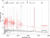 |
Fig. A.1 Comparsion between our Nov. 11, 2013 spectra at the onset of episode 2013A and a model spectrum of an LBV in quiescence with L = 1 × 10⁶L⊙, Teff = 8500 K, a mass loss rate of Ṁ = 5 × 10⁻⁴M⊙ yr-1 and a wind terminal speed of 600 km s-1. The model spectrum was downgraded to the resolution of the observed spectrum. The lines present are mainly Balmer lines, NaD, Ca II and Fe II. |
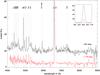 |
Fig. A.2 Late time spectra of SN 2009ip: at +581d (May 6, 2014) taken with EFOSC at the NTT (PESSTO data release, black) and at +1176d (Dec. 23, 2015) taken with Magellan-Clay (red). The inset shows the Hα line at the two epochs. |
Log of the photometric observations.
All Tables
All Figures
|
Fig. 1 Left: NGC 2770 observed with VLT (+FORS1) in January 2008, while there were two active SNe. An earlier SN from 1999 is indicated by a circle. Right: In May 2015 the SNe are gone in this image from GTC (+OSIRIS), but there is a new object, SN 2015bh, an LBV that potentially suffered a terminal explosion as a SN IIn. |
| In the text | |
|
Fig. 2 Top: light curve of the progenitor of SN 2015bh from 1994 until 2016, the insets are blow-ups of episode 2008 in different colors and episodes 2015A&B (main event and precursor). SN 2009ip is also displayed for comparison and shows a very similar behavior. |
| In the text | |
|
Fig. 3 Spectroscopic evolution of the LBV and SN, including two epochs during the LBV outbursts (episode 2013, –559 d and episode 2015A at –39 d) and a closely sampled time-series during the possible SN explosion from May 16 to June 19 (–7 to +27 d). After a gap in the observations due to sun constraints we obtained four new spectra in late September (+126 d), November 2015 (+181 d), December (+195.4 d) and January 2016 (+242 d). |
| In the text | |
|
Fig. 4 Optical spectrum at 6 representative epochs and line identifications. Not all lines are visible in all epochs. The grey bars indicate atmospheric lines. Color coding of the spectra is the same as in Fig. 3 |
| In the text | |
|
Fig. 5 Light curve in different bands during the main episode (2015B) and polynomial fits to the LCs. Grey arrows indicate the dates where we obtained spectroscopy. |
| In the text | |
|
Fig. 6 Temperature and radius evolution of the BB fitted to the SED during the main event (see Fig. 7). In the top panel we plot the bolometric LC for comparison. |
| In the text | |
|
Fig. 7 SED from UV to IR from the precursor (one epoch), during the main explosion event until 180 days post maximum. The fit shown is a simple BB fit with varying temperatures. For the VIS bands we derive magnitudes using the flux calibrated spectra. In the last spectrum/SED, the R-band is clearly affected by the strong relative Hα line flux at that time. |
| In the text | |
|
Fig. 8 Bolometric LC of the precursor (episode 2015A) and the main explosion event of SN 2015bh (epoch 2015B). As comparison we also plot the bolometric LC of SN 2009ip obtained in the same way as for 2015bh. |
| In the text | |
|
Fig. 9 Components fitted to the Hα and Hβ line at different representative epochs. The colors of the components are identical to the ones in Fig. 10: red/orange are the narrow P Cygni profile emission and absorption components, blue/turquoise the broad components and green the total fitted profile. |
| In the text | |
|
Fig. 10 Properties of Hα and Hβ derived from the component fits during the LBV phase, precursor and the main event. From top to bottom: total luminosity, velocity shift and FWHM and flux of the different components. Round symbols correspond to absorption components, triangles to emission components. Colors correspond to the components fitted as shown in Fig. 9. |
| In the text | |
|
Fig. 11 Hα EW evolution from the LBV phase to the possible SN explosion. For comparison we also show the EW evolution for SN 2009ip and several there type IIn SNe (data from Smith et al. 2014, and F. Taddia, priv. comm.) |
| In the text | |
|
Fig. 12 Balmer decrement evolution using total integrated and peak fluxes of Hα and Hβ and comparison with SN 2009ip (data from Levesque et al. 2014, who uses peak flux values, and Fraser et al. 2015). |
| In the text | |
|
Fig. 13 Sketch of the event during the LBV phase, after maximum brightness and at late times (>120 d) together with the corresponding profiles of Hα. The LBV is embedded in a dense CSM indicated by the grey shaded area. During the LBV phase, only one absorption component is present while post maximum, after the emission starts to fade, a second component becomes visible in all emission lines which we therefore attribute to a shocked region associated to the shell ejection or SN explosion. At late times, the second component shows up in emission, either implying that the second shell has interacted with CSM (probably the earlier ejected shell) or that is has become optically thin. |
| In the text | |
|
Fig. 14 Model fit to the bolometric LC and temperature evolution. |
| In the text | |
|
Fig. 15 HR diagram showing the evolution of SN 2015bh during the early outbursts, throughout the precursor, main event and decline (red dots). The boxes indicate the region in which SN 2015bh was located during different phases of the evolution. Blue dots show the same for SN 2009ip from 2009 to 2015 (data from Pastorello et al. 2013; Fraser et al. 2015). The last observation at –9.1 mag (R-band) is below the proposed progenitor level from HST observations in 1999 (blue dotted line, no color information is available for this epoch). We also plot data for Eta Carinae (Rest et al. 2012) today and during the main eruption as well as the range of LBVs between quiescence and outburst. |
| In the text | |
|
Fig. 16 The galactic environment of SN 2015bh in Hα, metallicity, Hα EW and specific SFR as observed with OSIRIS/GTC and drift-scan spectroscopy. The area covers about 5 × 2.5 kpc. Contours are from the TF observations of the Hα line. Note that the properties at the explosion site (marked by a cross) cannot be considered as the data are contaminated by emission from the LBV during outburst. |
| In the text | |
|
Fig. 17 Evolution throughout the HR diagram for several other events: The SN impostors SN 2008S, SN 2000ch and SNhunt248 and the type IIn SNe 1998S and 2010jl. Colored boxes correspond to the three main epochs of SN 2015bh as in Fig. 15. SN 2000ch occupies a very similar region to SN 2009ip and SN 2015bh in the LBV phase and could be a similar star in this pre-main event period. SN 2008S was always redder than SN 2009ip and SN 2015bh at much lower luminosities. SN 2010jl and SN 1998S reached higher magnitudes than the main events for SN 2009ip and SN 2015bh. SNhunt248 occupies a similar region during the outburst phase but has a lower luminosity at peak. The small late blue turn corresponds to a bump in the LC past maximum. |
| In the text | |
|
Fig. 18 Comparison between the spectra of SN 2015bh (black), SN 2009ip (blue), SN 1998S (a genuine type IIn), SN 2008S (an impostor) and SN at different epochs. Unfortunately, there are no spectra publicly available on SN 2009ip during the outburst phase, the same applies to the very similar event SNhunt 248 (Kankare et al. 2015; Mauerhan et al. 2015). |
| In the text | |
|
Fig. A.1 Comparsion between our Nov. 11, 2013 spectra at the onset of episode 2013A and a model spectrum of an LBV in quiescence with L = 1 × 10⁶L⊙, Teff = 8500 K, a mass loss rate of Ṁ = 5 × 10⁻⁴M⊙ yr-1 and a wind terminal speed of 600 km s-1. The model spectrum was downgraded to the resolution of the observed spectrum. The lines present are mainly Balmer lines, NaD, Ca II and Fe II. |
| In the text | |
|
Fig. A.2 Late time spectra of SN 2009ip: at +581d (May 6, 2014) taken with EFOSC at the NTT (PESSTO data release, black) and at +1176d (Dec. 23, 2015) taken with Magellan-Clay (red). The inset shows the Hα line at the two epochs. |
| In the text | |
Current usage metrics show cumulative count of Article Views (full-text article views including HTML views, PDF and ePub downloads, according to the available data) and Abstracts Views on Vision4Press platform.
Data correspond to usage on the plateform after 2015. The current usage metrics is available 48-96 hours after online publication and is updated daily on week days.
Initial download of the metrics may take a while.