| Issue |
A&A
Volume 686, June 2024
|
|
|---|---|---|
| Article Number | A231 | |
| Number of page(s) | 13 | |
| Section | Stellar structure and evolution | |
| DOI | https://doi.org/10.1051/0004-6361/202348679 | |
| Published online | 14 June 2024 | |
Searching for precursor activity of Type IIn supernovae
1
INAF – Osservatorio Astronomico di Brera, Via E. Bianchi 46, 23807 Merate (LC), Italy
e-mail: This email address is being protected from spambots. You need JavaScript enabled to view it.
2
INAF – Osservatorio Astronomico di Padova, Vicolo dell’Osservatorio 5, 35122 Padova, Italy
3
Instituto de Astrofísica, Universidad Andres Bello, Av.da República 252, 8320000 Santiago, Chile
4
Millennium Institute of Astrophysics, Nuncio Monsenor Sótero Sanz 100, Providencia, 8320000 Santiago, Chile
5
Instituto de Alta Investigación, Universidad de Tarapacá, Casilla 7D, Arica, Chile
6
University of North Carolina at Chapel Hill, Campus Box 3255, Chapel Hill, NC 27599-3255, USA
Received:
20
November
2023
Accepted:
14
March
2024
Abstract
We conducted a search for luminous outbursts prior to the explosion of Type IIn supernovae (SNe IIn). We built a sample of 27 objects spectroscopically classified as SNe IIn and all located at z < 0.015. Using deep archival SN fields images – taken up to nearly 20 yr prior to the SN explosions themselves – from transient surveys (PTF, ZTF, DES and CHASE) and major astronomical observatories (European Southern Observatory, ESO and National Optical Astronomy Observatory, NOAO), we found at least one outburst years to months before the explosion of seven SNe IIn, with the earliest precursor being 10 yr prior to the explosion of SN 2019bxq. The maximum absolute magnitudes of the outbursts range between −11.5 mag and −15 mag, and the eruptive phases last for a few weeks to a few years. The g − r colour measured for three objects during their outburst is relatively red, with g − r ranging between 0.5 and 1.0 mag. This is similar to the colour expected during the eruptions of luminous blue variables. We note that the light curves of SNe with pre-SN outbursts have faster decline rates than those of the SNe that do not show pre-SN outbursts. SN 2011fh is remarkable, as it is still visible 12 yr after the luminous SN-like event, indicating that the progenitor possibly survived, or that the interaction is still ongoing. We detect precursor activity in 29% of bona fide SNe IIn in our sample. However, a quantitative assessment of the observational biases affecting the sample suggests that this fraction is an underestimation of the intrinsic precursor occurrence rate.
Key words: supernovae: general / supernovae: individual: SN 2011fh / supernovae: individual: SN2016aiy / supernovae: individual: SN 2016cvk / supernovae: individual: SN 2019bxq / supernovae: individual: SN2019fmb
© The Authors 2024
 Open Access article, published by EDP Sciences, under the terms of the Creative Commons Attribution License (https://creativecommons.org/licenses/by/4.0), which permits unrestricted use, distribution, and reproduction in any medium, provided the original work is properly cited.
This article is published in open access under the Subscribe to Open model. This email address is being protected from spambots. You need JavaScript enabled to view it. to support open access publication.
1. Introduction
Supernovae (SNe) IIn are a class of explosive astrophysical events whose spectra show evidence of interaction between the fast SN ejecta and the slow, high-density surrounding material. The interaction is marked by the presence of narrow emission lines of the Balmer series, whose profiles are composed of a narrow component, sometimes with a P Cygni profile, on top of a broader one (Schlegel 1990; Filippenko 1997; Fraser 2020). The narrow component arises from slow-moving (∼102 km s−1) circumstellar medium (CSM) produced by the progenitor during previous mass-loss events, that is piled up around it. The broad component is generated by the fast-moving (∼104 km s−1) SN ejecta. The collision of the ejecta with the CSM generates two shock fronts, one moving inwards through the ejecta and the other outwards through the CSM, with the shocked material producing high-energy photons that ionise the CSM. The narrow spectral features are produced from the recombination of the slow-moving ionised gas. Other typical characteristics of SNe IIn are their high luminosity, which is produced by the efficient conversion of the kinetic energy of the ejecta into radiation, and the blue colours due to the high temperature of the gas, which are sometimes accompanied by a UV/X-ray excess (Chevalier & Fransson 1994).
In numerous cases, the progenitors of SNe IIn show signatures of strong variability, in the years prior to the explosion, including recurrent outbursts (e.g. Smith et al. 2010; Ofek et al. 2013; Tartaglia et al. 2016; Elias-Rosa et al. 2016, 2018; Thöne et al. 2017; Pastorello et al. 2018, 2019; Reguitti et al. 2019). The eruptive phases last from a few weeks to a few years (see Smith et al. 2011). These pre-SN events belong to the stellar transient category of “SN impostors” (Van Dyk et al. 2000), because their spectra and evolution in some cases can resemble those of a Type IIn SN. However, SN imposters are less luminous, with absolute magnitudes ranging between −10 and −15 mag, and belong to the population of the so called “gap transients” (Kasliwal 2012; Pastorello & Fraser 2019; Cai et al. 2022). Eruptive mass-loss events from luminous blue variables (LBV, Humphreys & Davidson 1994) are a plausible explanation of the SN impostor phenomenon (Gal-Yam et al. 2007; Gal-Yam & Leonard 2009, but see Smith 2017).
Ofek et al. (2014, hereafter O14) conducted a systematic search for precursor transient events that later produced Type IIn SNe. These authors inspected archival Palomar Transient Factory (PTF; Law et al. 2009) images of 16 objects, taken between 1 and 3 yr before the explosion, and found luminous outbursts for six of them. From this result, they also estimated that about 50% of Type IIn SNe are expected to experience at least one luminous outburst (brighter than MV = −14 mag) within the 4 months prior to the terminal explosion. In contrast, Bilinski et al. (2015, hereafter B15) conducted a similar search for 6 SNe IIn with archival Lick Observatory Supernova Search (LOSS; Filippenko et al. 2001) data from the 76 cm Katzman Automatic Imaging Telescope (KAIT) telescope taken up to 12 yr prior to the SN explosions, but these authors found no precursors. This latter result can be explained by the limited sample and the low limiting magnitude achieved by the survey (around 19 mag).
More recently, Strotjohann et al. (2021, S21) performed a similar search for a much larger sample of objects (196 interacting SNe) over images from the Zwicky Transient Factory (ZTF; Masci et al. 2019) Survey taken between March 2018 and June 2020. These authors retrieved precursor eruptions prior to 18 Type IIn SNe and one Type Ibn SN, and found that the precursor events become brighter and more frequent in the last months before the SN. Furthermore, S21 found that a quarter of all Type IIn SNe experience month-long outbursts brighter than an absolute magnitude of −13 mag within the final three months before the explosion. The radiative energies of the outbursts are up to 1049 erg.
In this paper, we present the results of our independent search for pre-SN outbursts conducted for a sample of 27 Type IIn SNe discovered within about 60 Mpc. We made use of archival images from major astronomical observatories, like the European Southern Observatory (ESO) and the National Optical Astronomy Observatory (NOAO), as well as frames collected by public photometric surveys, such as PTF, ZTF and the Dark Energy Survey (DES1; Abbott et al. 2018). Our research differs from previous investigations in our contemporary use of archival data from both surveys and observatories, with the latter being much deeper in some cases (down to ∼22.5 mag) – allowing us to detect outbursts as faint as Mr ∼ −11 mag – and obtained over longer timescales (up to 10 yr before the SN explosion).
The structure of the paper is as follows: in Sect. 2, we present the sample of Type IIn SNe and the adopted selection criteria. In Sect. 3, we describe the methodology of the investigation and the adopted data-reduction techniques. The principal results are outlined in Sect. 4, followed by a discussion in Sect. 5. Finally, our conclusions are presented in Sect. 6.
2. The sample
We searched for all objects classified as a Type IIn SN in the Transient Name Server (TNS2), the Weizmann Interactive Supernova Data Repository (WISeREP3, Yaron & Gal-Yam 2012), and the Asiago Supernova Catalogue4 (Barbon et al. 1989, 1999) databases, up until April 2021, and with a redshift of z < 0.015, retrieving 82 SNe. Assuming a standard cosmology (H0 = 73 km s−1 Mpc−1, Ωm = 0.27, ΩΛ = 0.73; these cosmology parameters are adopted throughout this paper), this corresponds to a distance of about 61.6 Mpc, or a distance modulus (DM) of 34 mag. We chose this limit as the typical absolute magnitude of the pre-explosion outbursts is ∼ − 13 to −14 mag (Smith et al. 2011, O14), and the limiting apparent magnitude of modern surveys is in the 19–21 mag range (see Sect. 3).
However, inspection of the information available in the literature revealed that some objects, initially classified as SNe IIn, were instead other types of transients. In particular, Ransome et al. (2021) revised the classification of a large sample of transients previously identified as SNe IIn. This allowed us to exclude gap transients (Pastorello & Fraser 2019) and SNe misclassified as Type IIn from our sample. Flash spectroscopy SNe (Gal-Yam et al. 2014; Bruch et al. 2021) were also removed from the sample, as they show high ionization lines (from C III, C IV, N IV) which are rarely (if ever) observed in Type IIn SNe. These features remain visible only for a few days before disappearing as the object evolves as a normal Type II SN: an example is the notable case of SN 2020tlf (Jacobson-Galán et al. 2022). Instead, true SNe IIn show narrow H lines throughout their entire evolution, which can even last for years. Finally, we only considered objects for which at least some pre-explosion images are available. We note that hundreds of images are available for some objects, while for others there are only a few.
The final sample of 27 SNe IIn is presented in Table 1. A search for pre-SN activity for one object in our sample, SN 2013gc, was already presented in Reguitti et al. (2019), who found at least one eruptive episode before the explosion in PTF data. SN 2010jl was also included in the samples of O14 and B15, while SNe 2019bxq and 2019fmb were included in S21. Three other SNe in our sample are in common with that of B15: SNe 1999el, 2008fq, and 2011A. Moriya et al. (2023) recently studied the environments of a sample of SNe IIn, and included SNe 2016aiy and 2016cvk. During the advancement of this research, the nearby Type IIn SN 2021foa exploded, which fullfills the requirements to be included in our sample. We conducted a dedicated analysis of this object and a search for precursors. While we did not find evidence of pre-SN activity in the archives listed above, the Asteroid Terrestrial-impact Last Alert System5 (ATLAS; Tonry et al. 2018) observed an early rise and a bump in the light curve two weeks before discovery of the SN, which is compatible with an Event A from a SN 2009ip-like object. An individual study of SN 2021foa was presented by Reguitti et al. (2022). In Sect. 4, we provide a detailed description of the objects for which we detected pre-SN activity, while the rest of the sample is used in Sect. 5 to estimate the rate of the precursors.
Our sample of 27 Type IIn SNe.
3. Methodology and data reduction
Because the eruptive episodes are expected to be faint, and hosted in complex environments in their host galaxies, we adopted the template-subtraction technique. We used a dedicated pipeline called SNOoPY6 (Cappellaro 2014), which allows us to perform the alignment, transformation, and PSF matching of the template to the science images. The instrumental magnitudes were determined through the PSF fit measurement performed on the template-subtracted images. For Sloan-filter images, the photometric zero points and colour terms were computed with a sequence of reference stars from the Panstarrs DR17 (PS1; Chambers et al. 2016) survey in the SN field. For the few objects with δ < −30°, whose fields are not covered by the PS1 survey, we constructed a local sequence of stars from the APASS DR10 catalogue8 in the Sloan gri filters. APASS DR10 was also used to calibrate the Johnson BV filters frames. We calibrated the few photometric points obtained with Johnson RI filters as Sloan ri magnitudes. Small deviations in magnitude of a few hundredths of a magnitude in the magnitudes can arise because of this approximation. Photometric errors were estimated through artificial star experiments9, where uncertainties in the PSF-fitting procedure are also accounted for. Clear filter magnitudes were usually scaled to Sloan-r magnitudes, because the quantum efficiency of the detector peaked at a wavelength near the response peak of that filter, while those of SN 2011fh were scaled to Johnson V magnitudes. We adopted a rather loose constraint on the signal-to-noise ratio (S/N) of higher than 3 (instead of 5 as used by S21) for a source at the expected SN position in the template-subtracted image to be counted as securely detected. We note that, in any case, the presence of an outburst is confirmed by several detections.
We made use of reference frames (templates) without any signature of a source at the SN location down to their limiting magnitudes. These templates are then subtracted from our science frames in order to remove the contamination of the host galaxy. For the Sloan-filter images, we used the stack10 PS1 images as templates, while for the B and V frames we used the stack PS1-g band images. For the R and I images, we adopted PS1-r and PS1-i templates, respectively. The mismatch between the Johnson and Sloan filters’ response curves may introduce an additional error in the final magnitude depending on the colour of the source. However, this error does not influence detectability, and only slightly changes the upper detection limits. Finally, for southern objects we used the best-quality (in terms of seeing and exposure time) images available in the public archives as templates. Instead, for SNe 2016cvk and 2016aiy, we used aperture photometry, as a source is always visible at the SN position in the deepest images.
We searched for pre-explosion images in the public archive of the PTF11 and ZTF12 surveys, which scanned the sky with a regular cadence and have a long time coverage. Both surveys operate with the 1.2 m Samuel Oschin Telescope at the Palomar Observatory and monitor the entire northern sky (δ ≳ −30°) every few days. PTF operated between March 2009 and December 2012, mostly with a Johnson-R filter, but also with a Sloan-g filter. The standard exposure time per frame is 60 s, yielding a 5σ limiting magnitude of 20.5 and 21 mag for R- and g-band, respectively. ZTF started operations in early 2018, and with Data Release 7, all images taken until June 2021 are publicly available. ZTF routinely observed with the Sloan g and r filters, but occasionally observations were also performed in Sloan i. ZTF used a camera with a 47 square degree field of view and was able scan more than 3750 square degrees per hour to a depth of 20.5 mag (Bellm et al. 2019). We also searched for images available in the archive of the CHilean Automatic Supernova sEarch survey (CHASE, PI Pignata; Pignata et al. 2009), which operated with the Panchromatic Robotic Optical Monitoring and Polarimetry Telescopes (PROMPT; Reichart et al. 2005) at the Cerro Tololo Inter-American Observatory (CTIO). The survey was primarily made with an Open filter and had a 3σ limiting magnitude of 19–19.5 mag. Lastly, the DES survey, which operates with the DECam camera mounted at the 4 m Blanco telescope at CTIO, also provided a few pre-explosion images. The cadence of the DES survey is lower compared to those dedicated to transient searches, but operating with a much larger telescope it is able to reach a limit of 22.5–23 mag. PTF monitored the fields of 11 objects in our sample before the explosion, while ZTF monitored the fields of 5 objects, CHASE 10 targets, and DES 3 targets.
Along with the archives of the public surveys PTF, ZTF, DES, and CHASE, we searched for pre-explosion images in the archives of major astronomical observatories worldwide. A drawback of the observatory archives is that the images, when available, are few and are sparse in time. Nonetheless, in some cases, these images are deeper than those from the surveys, as they were taken with larger telescopes and/or with longer exposure times. This allowed us to put more stringent constraints (upper limits) on the brightness of the progenitor during the quiescent phases. For instance, around 10 yr before the explosion of SN 2011A, its progenitor was fainter than MR = −10.6 mag, while in 2016 (3 yr before the precursor activity we spotted) the progenitor of SN 2019fmb was dimmer than Mg = −10.9 mag, and finally from a deep DES image we can rule out that in 2016 the progenitor of SN 2019esa was brighter than Mr = −10.5 mag (see last column of Table 1). Table B.1 provides some information on the facilities that provided archival data. Photometric tables with the magnitudes of the pre-SN detections and non-detections are available on a dedicated website13.
4. Results
In this section, we provide further details of five of the seven SNe for which we detected a precursor activity. SNe 2013gc and 2021foa were presented in Reguitti et al. (2019 and 2022), respectively.
4.1. SN 2011fh
SN 2011fh was discovered by Berto Monard on 2011 August 24 (Monard et al. 2011) in the spiral galaxy NGC 4806 (DM = 32.59 mag) at an unfiltered magnitude of 14.5. From the analysis of archive images, the object became gradually brighter from February 2011 (at 17.0 mag) to August 2 (at 16.0 mag; this is the last observation prior to discovery). An optical spectrum was obtained 5 days after discovery at the du Pont 2.5 m telescope at Las Campanas Observatory. The spectrum shows a blue continuum and strong emission lines from the Balmer series with multiple velocity components, typical of a Type IIn SN (Monard et al. 2011).
The CHASE observed the field from April 2008, and followed it until March 2015. In this case we calibrated the unfiltered images to the V-band photometry. The transient shows an overall rise with some fluctuations in the 3 yr prior to the discovery. The luminosity increased with time, from a mean magnitude of 18.2 mag in 2008 to 18.0 mag in 2009 and 2010. Between January and May 2011 the object further brightened from 17.5 to 17.0 mag, and finally in Summer 2011 a major brightening marks the start of the brightest event, which is the putative Type IIn SN explosion.
The CHASE survey resumed observing SN 2011fh on 7 January 2012, when the transient had already dimmed to mag 17.1, continuing to fade with a slower rate of decline. In March 2015 (nearly 4 yr after the explosion), the object was still recovered at V = 18.8 mag, slightly fainter than the luminosity level the source was spotted at in 2008. In 2016 (5 yr after discovery), the Hubble Space Telescope (HST) observed the field of NGC 4806 with the WFC3 camera in the F336W and F814W filters (P.I. Filippenko). A bright source was clearly visible within 0.1″ of the location of SN 2011fh. From that image, we measured F814W = 19.8 ± 0.1 mag, indicating a clear flattening of the light curve. The transient was still detectable in March 2018 in an archival white-filter LCOGT image at R ≃ 19.0 ± 0.2 mag, and even more recently in February 2021 and March 2023 in an unfiltered PROMPT image at V = 20.0 ± 0.16 and V = 20.1 ± 0.14 mag, respectively. All our data are shown in Fig. 1.
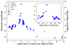 |
Fig. 1. Pre- and post-discovery observation of SN 2011fh. Clear filter magnitudes from the CHASE Survey and from amateurs are plotted as V-band, a single w-band LCOGT observation as R-band, and the 2016 HST F814W observation as I-band. Observations from different instruments are plotted with different symbols. The late-time luminosity level is marked with a dashed line. A zoom onto the rise to the 2011 event is plotted in the inset window, showing the first year of decline, during which a second, smaller peak is visible at +250 days. |
In their paper, Pessi et al. (2022) studied SN 2011fh in detail. Their photometric data cover the 2007–2013 period, and their r-band light curve is very similar to our V-band light curve. These authors concluded that SN 2011fh shares common features with the Type IIn SN 2009ip (Mauerhan et al. 2013a; Pastorello et al. 2013; Margutti et al. 2014; Smith et al. 2014), and attribute the HST detection at +5 yr to an ongoing ejecta-CSM interaction or to an eruptive phase. A MUSE spectrum at the Very Large Telescope (VLT) of the field of SN 2011fh indeed shows signs of interaction at nearly +4 yr. Other members of the SN 2009ip-like family of objects have recently been confirmed as genuine terminal SNe events, as they continued to fade below the progenitor level after the brightest event (Smith et al. 2022; Jencson et al. 2022; Brennan et al. 2022a). Fransson et al. (2022) propose multiple scenarios to explain SN 2009ip-like events: a pulsational pair instability SN (Woosley et al. 2007); a large mass eruption followed by a normal SN explosion from a lower mass (≲20 M⊙) progenitor; or a merger of a massive star with a compact object. In contrast, SN 2011fh is still visible after more than 10 yr, although it is slightly fainter than 3 yr before the 2011 event.
On 10 August 2023 (12 yr after maximum) we obtained a spectrum of SN 2011fh with the 6.5 m Clay telescope, which was reduced, extracted and calibrated using routine IRAF procedures. The final spectrum is shown in Fig. 2. Overall, the spectrum does not show significant evolution from the +4 yr MUSE spectrum published by Pessi et al. (2022), in accordance with the extremely slow evolution of the light curve at very late phases. He I lines are present, with a full width at half maximum (FWHM) velocity comparable to that of the broader component in the Hα line (1500–2000 km s−1). The FWHM of the He I lines is 1700 km s−1, which is compatible with the velocity of a fast outflow from an early Wolf–Rayet star (Smith 2017). The [O I] and [Ca II] doublets are absent or very faint, suggesting that the progenitor star survived the 2011 event, making SN 2011fh a luminous SN impostor.
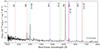 |
Fig. 2. Spectrum of SN 2011fh taken with the 6.5 m Clay telescope+LDSS3 12 yr after maximum light. The principal identified emission lines are marked. |
4.2. SN 2016aiy
The discovery of SN 2016aiy (ASASSN-16bw) was made by the All Sky Automated Survey for SuperNovae (ASAS-SN; Shappee et al. 2014) on 2016 February 17 (Brimacombe & Holoien 2016) in the galaxy ESO 323-G084 (DM = 33.07 mag) at V = 16.9 mag. However, a detection from ASAS-SN was obtained 2 days earlier, at V = 17.2 mag. The last non-detection is on February 11, at V > 18.2 mag. SN 2016aiy was classified as a SN IIn on 2016 February 24 by the PESSTO Collaboration (Taubenberger et al. 2016).
The field of SN 2016aiy was monitored before the explosion only by the DES Survey between March 2013 and June 2015. We have only four epochs of sparse griz photometry, and in three of them we measure a source with a magnitude of between 21.6 and 22.6 mag. In particular, the object was detected three times in the r-band at the extremes of the monitoring temporal window at an Mr of between −10.8 and −11.8 mag; see Fig. 3.
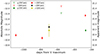 |
Fig. 3. Pre-discovery griz observations of SN 2016aiy from the DES survey. The phases are relative to the V-band maximum (Reguitti et al., in prep.). |
We conclude that we are observing the progenitor in an active state or in outburst, because the source is variable and a −11 mag star in quiescence is less plausible. We can rule out a variable stellar source within a luminous stellar cluster, because at a very late time (+3 yr) we do not detect any source brighter than 22.8 mag in profound images from the NTT telescope, an upper limit which is fainter than the pre-SN detections (Reguitti et al., in prep.). The post-explosion light curves and spectral evolution of SN 2016aiy – along with their connection to the observed pre-SN activity – will be presented in a forthcoming paper (Reguitti et al., in prep.).
4.3. SN 2016cvk
SN 2016cvk was discovered by the Backyard Observatory Supernova Search (BOSS) team on 2016 June 12 (Parker 2016) in the galaxy ESO-344-G21 (DM = 33.21 mag), at an unfiltered magnitude of 17.6. The last non-detection is on 3 June 2016, with a limiting magnitude of 18.0. The ASAS-SN Survey discovered a second transient at the location of SN 2016cvk on 2016 August 31, at V ∼ 16.2 mag, identified with a survey name of ASASSN-16jt (Brimacombe et al. 2016). A non-detection (V > 17.8 mag) 5 days before discovery was also reported by Brimacombe et al. (2016). The position of the new transient was within 1″ of the position reported in June 2016. For this reason, we are confident that the location of the two transients is coincident, and that the event observed in June 2016 was a previous outburst of an object that later exploded as a SN (see also Brown et al. 2016). The classification spectrum of ASASSN-16jt/SN 2016cvk was taken 3 months later, on 6 September, by the PESSTO Collaboration (Smartt et al. 2015) with the 3.58 m ESO-NTT telescope. The new object was classified as a peculiar SN IIn (Bersier et al. 2016). However, a previous spectrum was taken on 18 June (during the outburst) at the du Pont 2.5 m telescope (Brown et al. 2016), and was found to be similar to the spectrum of SN 2009ip before its peak in September 2012. This, and the photometric evolution observed during Summer 2016, make SN 2016cvk a promising SN 2009ip-like candidate. An extended analysis of the post-explosion light curve and spectral evolution will be presented in a future paper (Matilainen et al., in prep.).
The CHASE project monitored the field of SN 2016cvk between October 2010 and December 2013. We find no further detections in those images, apart from a single detection on 2013 May 12 at 19.25 ± 0.16 mag (calibrated as Sloan-r). At the assumed distance of ESO-344-G21, this photometric point gives an absolute magnitude of Mr ∼ −14.0 mag. Starting from November 2013, the DES survey targeted the same region of sky in Sloan-grizy, until July 2015. Thanks to the large diameter of the telescope, DES can provide much deeper photometry. Indeed, in all but one image, we detect a faint source at the SN location (between 20.3 and 21.5 mag) in the griz filters. The pre-discovery absolute light curve is shown in Fig. 4.
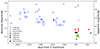 |
Fig. 4. Pre-discovery light curves of SN 2016cvk. The clear filter observations from the CHASE are in blue, and the other points are with Sloan filters from the DECam instrument. The open inverted triangles are upper limits, and the filled circles are detections. The larger triangles with a horizontal error bar indicate more profound upper limits derived from stacked frames within the temporal bar. The phases are relative to the V-band maximum (Matilainen et al., in prep.). |
4.4. SN 2019bxq
SN 2019bxq (ZTF19aamkmxv; PS19ahx) was formally discovered by the ZTF survey on 15 March 2019 (Nordin et al. 2019) in the galaxy LEDA 84787. According to the NASA Extragalactic Database (NED14), the host is an Elliptical Star-Forming galaxy. The classification spectrum, taken at the Palomar 5 m Hale telescope about one month after the discovery, shows numerous narrow emission lines, including those from the Balmer series, over a still blue continuum, making SN 2019bxq a Type IIn SN (Fremling et al. 2019). The host redshift reported by NED, of z = 0.01421, is consistent with that obtained from the classification spectrum (z = 0.014). Using the former z estimate, we derive a kinematic distance modulus DM = 33.83 mag. The adopted Galactic reddening is AB, MW = 0.181 mag (Schlafly & Finkbeiner 2011); using the Cardelli et al. (1989) extinction law, we derive a reddening in the R-band of AR, MW = 0.11 mag.
SN 2019bxq was part of the S21 sample, and that study found precursor activity in the ZTF images. Furthermore, we observed multiple eruptive episodes in the PTF data from 2009 to 2011. As shown in Fig. 5, there are multiple detections, which can be divided into four main eruptive events. The first event began 3571 days (∼9.8 yr) before the SN maximum light, and lasted around 3 months. This was the best sampled outburst, and from the brightest detection (R = 19.08 ± 0.12 mag) we can infer a maximum absolute magnitude of the outburst of MR, max = −14.8 mag (see also Fig. 5). After the seasonal gap, the object became visible again. We detected the object in outburst for the second time during the luminosity rise, reaching a similar maximum absolute magnitude of MR, max = −14.5 mag, before declining. For a few weeks, the transient was not detected above the limiting magnitude threshold of our images. Later, the object was newly detected during its third outburst. Finally, after a long interruption due to the solar conjunction, we detected the object during a fourth outburst. The last points were obtained before the end of the PTF survey operations. Finally, we also recovered sparse detections from the ZTF data in the final year before the explosion, as already spotted by S21.
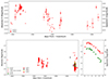 |
Fig. 5. Pre- and post-explosion light curves of SN 2019bxq. Top: Pre-explosion R-band absolute light curve of SN 2019bxq from the PTF survey. The data span the 2009–2011 period. The magnitudes are corrected for the adopted distance modulus and Galactic reddening. The phase on the x-axis is from the SN r-band maximum (MJD = 58577). The open inverted triangles mark upper limits (i.e. non-detections). Bottom left: Same as above, but including all the available data (PTF+ZTF+sparse archive data). Observations from different instruments are plotted with different symbols. The phases are relative to the brightest r-band point in the SN light curve. Bottom right: Post-explosion g- and r-band light curves of SN 2019bxq from the ZTF survey. The SN light curves are shown to highlight the short duration of the SN event. |
4.5. SN 2019fmb
SN 2019fmb (ZTF19aavyvbn; ATLAS19bbhu; PS19ahl) was discovered by the PS1 survey on 12 May 2019 (Chambers et al. 2019), in the galaxy LEDA 40731. The classification spectrum, taken at the 3.5 m APO telescope about 6 months after discovery, shows narrow Hα emission over a continuum that is still quite blue. For this reason, SN 2019fmb was classified as a Type IIn SN (Graham et al. 2020). These latter authors deduced a redshift of z = 0.016 from the Hα emission, and we therefore adopt DM = 34.09 mag. The Galactic reddening is negligible, at Ar, MW = 0.036 mag.
Analysing the ZTF data of SN 2019fmb, we found numerous faint detections after the discovery epoch, with apparent magnitudes of between 20.0 and 21.5 mag, corresponding to absolute magnitudes ranging from −12.5 to −14.0 mag. Prediscovery detections were obtained thanks to the PS1 survey in the g, r, and also i bands. The absolute magnitude of the source in this phase suggests it was most likely an SN impostor. We observed three months of pre-SN activity, with the r-band luminosity gently increasing to a shallow maximum at around one month after the discovery, and the outburst luminosity slightly fading after that. About 100 days later, we detected the object twice in the g band, with the source becoming much brighter (Mg ∼ −14.5 mag) than during the previous activity. We argue that these detections mark the light curve rise to the maximum light (which was not observed) soon after the SN explosion. The SN luminosity decline was partially followed by the ATLAS survey (Fig. 6, right panel).
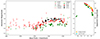 |
Fig. 6. Pre- and post-explosion light curves of SN 2019fmb. Left: Pre- and post-discovery (MJD = 58 615) Sloan-gri detections from the ZTF and PS-1 surveys of SN 2019fmb. Observations from different instruments are plotted with different symbols. The phases are relative to the brightest r-band point in the SN light curve. The deepest upper limits of the object in g-, r- and z-band filters from NOAO archival data of 2016 are marked with horizontal lines in the bottom-left corner. Right: Light curve of SN 2019fmb, with the detections by ATLAS also reported. As for SN 2019bxq, the SN has a short duration. |
The light-curve hump observed before the explosion of SN 2019fmb is reminiscent of those observed before the explosion of other SNe IIn, specifically SN 2009ip-like events (e.g. SNe 2016bdu, Pastorello et al. 2018; LSQ13zm, Tartaglia et al. 2016; 2016jbu, Brennan et al. 2022b; 2021foa, Reguitti et al. 2022). SN 2019fmb is also included in the sample of S21, and these authors noted similar photometric behaviour. The corresponding light curves are plotted at the top of Fig. 6.
We also found several older “Mosaic3+90prime” survey images taken in 2016 and 2017 in the NOAO Archive. While the transient is not detected in these images, we can establish an upper limit to the g-band quiescent progenitor magnitude, with Mg > −11 mag (Fig. 6, bottom left).
5. Discussion
Among the objects considered in our sample, SNe 2013gc, 2016aiy, 2016cvk, 2019fmb, and 2021foa each present one pre-SN outburst or prolonged activity, while SN 2019bxq shows four events, and SN 2011fh reveals a slow, year-long rise, which was also noted by Pessi et al. (2022). Hence, we observed ten luminous events before the 27 SNe in our sample.
As opposed to S21, the precursors in this work are detected not only close to the SN explosion, but also earlier (up to 10 yr prior to the SN explosion in the case of SN 2019bxq). Unstable ignition of advanced nuclear burnings in the core of massive stars is sometimes invoked as a powering mechanism for SN impostor events (Arnett & Meakin 2011; Quataert & Shiode 2012; Smith & Arnett 2014). Specifically, Shiode & Quataert (2014) show that in stars with M ≲ 20 M⊙ the Ne-burn can start 1–10 yr before the SN explosion, which is broadly compatible with the precursor activity observed prior to SNe 2019bxq, 2016aiy and 2016cvk. Wu & Fuller (2021, 2022) updated the models by Fuller (2017) and Fuller & Ro (2018), finding that the wave-driven heating is not strong enough to trigger mass loss in H-rich stars, and hence this mechanism is not able to explain the precursor of SNe IIn.
5.1. Precursor characterisation
Here we try to characterise the precursors of SNe IIn we found by analysing their observational properties, such as duration, luminosity, and colour, looking for common features. In general, the precursor activities we detected are not well sampled, and therefore we need to make significant assumptions regarding the shape of the burst light curve in order to characterise them to first order. With the purpose of limiting the complexity of the model, we assume that the flux evolution of each burst can be described with a Gaussian function with four free parameters: the amplitude (ap), the width (σp), the epoch of the maximum, and the background level. To increase the statistics, we collected the published magnitudes of other outbursts before Type IIn SNe that do not belong to our sample, namely SNe 2015bh (Elias-Rosa et al. 2016; Thöne et al. 2017), 2016bdu (Pastorello et al. 2018), 2018cnf (Pastorello et al. 2019), LSQ13zm (Tartaglia et al. 2016), 2010mc (Ofek et al. 2013), and 2011ht (Mauerhan et al. 2013b; Fraser et al. 2013). Among them, SNe 2016bdu and 2018cnf show two pre-SN bright events, which are treated as two separate outbursts. For all the precursors, the r- or R-band filter has the largest number of detections, abd therefore we focused our analysis on this band. We converted the apparent magnitudes to luminosity by adopting the distances and Galactic reddenings reported in Table 1 or in the relative papers. For each outburst, we performed the previously mentioned Gaussian fit over the luminosities with the curve_fit tool in Python. Upper limits were also used to constrain the fits. An example of a Gaussian fit on the data points of an outburst is shown in Fig. 7.
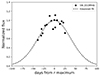 |
Fig. 7. Gaussian fit (dashed line) over the r-band light curve of the pre-SN outburst before SN 2019fmb. The magnitudes of the data points were converted into fluxes, and then normalised with respect to the peak of the Gaussian fit and centred on the epoch of the maximum. |
For each Gaussian best fit, we calculated the area 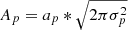 , which is the most characteristic parameter for statistical purposes. In physical terms, the area would be proportional to the total amount of energy released during the outburst. We can also define a mean luminosity during the outbursts by dividing the area of the Gaussian (
 ) by the maximum considered temporal length (6σp), obtaining
  , which is ≈0.95 mag fainter than the peak magnitude.
The background level was set to 1 million L⊙ (equal to Mr = −9.8 mag). This value was chosen as it is close to the estimated luminosity of the quiescent progenitors of the Type IIn SNe 2005gl (Gal-Yam et al. 2007; Gal-Yam & Leonard 2009) and 2009ip (Foley et al. 2011) identified in HST archival images as candidate LBVs.
The observed brightest absolute magnitudes of the precursors range between −11.5 and −14.8 mag, with an average of −13.7 ± 1.5 mag. The faintest detection of a precursor is for SN 2016aiy at Mr = −10.9 mag, thanks to the deepness of the DES survey images. Therefore, we do not find any precursor brighter than Mr −15 mag (excluding SN 2018lkg, which we assume not to be a SN IIn; see Appendix A). The range in magnitude of the single detections is −10.9 to −14.8, which is similar to but narrower than that of the events identified by S21 (from −12 to −17 mag). Our sample is smaller than that of S21; this may explain why we do not detect very bright outbursts. At the same time, we may also miss faint events because we did not stack our data.
We searched for a correlation between σp and ap of the Gaussians which can be interpreted as proxies for the duration and peak brightness of the burst, respectively, but we did not find any (Pearson correlation test: r = 0.11 and p-value = 0.69).
For three objects, pre-explosion outbursts were detected in more than one filter, allowing us to construct their colour curves. Because most of the outbursts were observed in recent years, multi-band observations are available in the Sloan-g, r, and i filters. This allows us to calculate the evolution of the g − r and r − i colours. We consider two observations in different filters obtained within less than 1 day of each other as contemporary. Figure 8 shows the g − r colour light curves of the outbursts of SNe 2016aiy, 2016cvk, and 2019fmb with respect to the epoch of maximum of the outbursts. The maximum light epoch of each outburst was estimated using Gaussian fits.
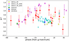 |
Fig. 8. g − r colour of the three pre-SN outbursts or activities for which multi-band photometry is available. The phases are relative to the maximum in the r-band, which was derived from a Gaussian fit over the data points. For comparison, the V − R colour of the 2000 and 2008 outbursts of the known LBV AT 2000ch (Pastorello et al. 2010) and of the SN impostor SN 2007sv (Tartaglia et al. 2015) are also shown. The g − r colour of the outbursts is red, around g − r∼0.5 mag. |
The g − r colours of the three outbursts are concentrated in the range of 0.5–1.0 mag. This red colour is compatible with that observed during the giant eruptions of LBV stars, whose spectra shift from those of B-types to cooler F-types (Humphreys & Davidson 1994). For example, during the 2014–2017 eruption of the LBV R40, it had B − V ≈ 0.6 mag (Campagnolo et al. 2018), corresponding approximately to g − r ≈ 0.5 mag (using the relations of Jester et al. 2005). In Fig. 8, the g − r colours of the outbursts are compared with the V − R colour of the SN impostor SN 2007sv (Tartaglia et al. 2015), together with the 2000 and 2008 bright events of the LBV known as AT 2000ch (Wagner et al. 2004; Pastorello et al. 2010). The colours are similar, especially those of the 2000 event. Focusing on the g − r colour curve of the precursor of SN 2019fmb, despite its relatively large error bars, we note that the colour shows an evolution during the outburst, passing from blue (g − r ∼ 0.5 mag) to red (1.0 mag) from the begin to the maximum, and then back to blue at the end of the burst.
The spectra of SN impostors and LBV eruptions are usually characterised by strong and narrow emission lines, with Hα being predominant. As the maximum of the response curve of the r filter is close to the wavelength of Hα, its flux may affect the g − r colour. To establish whether or not the Hα flux contribution can account for the red colours of the pre-SN outbursts, we collected the classification spectra of all the objects classified as SN impostors or LBV eruptions in the TNS and WISEReP databases (15 objects in total), and manually removed the Hα line in each of them. We then calculated the r-band synthetic photometry with the IRAF synphot tool, both with and without Hα included, and calculated the difference in magnitudes. In most cases, the difference is less than 0.3 mag; for three objects, it is around 0.4 mag and for just one the difference is 0.8 mag. A histogram of the distribution of the differences is shown in Fig. 9. The small differences indicate that the Hα emission can only partially justify the observed red g − r colours of the outbursts, and therefore these red colours are mostly due to a cooler continuum temperature, as seen in the LBV eruptions.
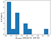 |
Fig. 9. Histogram of the distribution of the difference in the r-band synthetic photometry – with and without the Hα contribution – of the classification spectra for a sample of SN impostors and LBV eruptions. |
For the precursor of SN 2019fmb, it is possible to obtain the r − i and g − i colours as well. Its mean r − i colour is 0.5 mag, while the g − i colour is around 1.1 mag. The g − i value is higher than the 2008 outburst of AT 2000ch (which rose from 0.4 to 0.9 mag), and is the same as that found by S21, whose findings also agree with ours regarding the low effective temperatures of the precursors (∼4300 K for SN 2019fmb).
In summary, the outbursts we find are rather luminous (with absolute magnitudes in the −11 to −15 mag range) and are red in colour (with g − r from 0.5 to 1.0 mag), which is likely due to cool photospheric temperatures; these characteristics are analogous to those observed during LBV eruptions.
5.2. Connection between pre-SN outbursts and SN light curves
We investigated a possible impact that the pre-explosion activity could have on the properties of the SNe IIn after the explosion. For SNe 2019bxq and 2019fmb, we collected the publicly released gr light curves from the ZTF survey, which are available15 from the ALeRCE broker (Förster et al. 2021). For SN 2011fh, we used the images from the CHASE survey to also construct the post-explosion light curve. The light curves of SNe 2016ehw, 2017gas, and 2019esa were retrieved from the Gaia Photometric Science Alerts16. Finally, for SNe 2008fq, 2009au, 2010jl, 2010jp, and 2015da the light curves are collected from the respective publications (Taddia et al. 2013; Rodríguez et al. 2020; Zhang et al. 2012; Smith et al. 2012; Tartaglia et al. 2020).
The interaction between the SN ejecta and the material ejected during the precursor activity should modify the evolution of the light curve of the SNe, as the thermalisation of the kinetic energy from the ejecta into radiation through the interaction with the CSM should provide an additional powering source (Graham et al. 2014; Nyholm et al. 2017). Therefore, to investigate whether or not the precursor activity has a significant impact on the post-explosion behaviour, we measured the decline rates of the post-explosion light curves of the SNe in our sample during the first 65 days post explosion. Assuming that the material ejected during the outburst episodes has a maximum velocity of ∼1000 km s−1 and that SN ejecta expand at velocities higher than ∼10 000 km s−1, they should reach the material originating from the precursor activity as late as 65/0.1 = 650 days before the explosion. As visible in Fig. 1 and in Figs. 3–6, in all the SNe of our sample that show precursor activity, the last episode occurs closer to the explosion time frame than the previously mentioned time span. Therefore, if the precursor activity has a significant impact on the rate of decline of the SNe light curve, in principle it should be detectable in our sample.
In order to test this latter hypothesis, we constructed the cumulative distributions of the rates of decline for the SNe that did and did not show precursor activity in our data (see Fig. 10). The Kolmogorov–Smirnov test over the two cumulative distributions gives D = 0.61 and a p-value of 0.09, while the Anderson-Darling test provides A = 2.18 with a significance level of 0.04. The latter indicates that there is a marginally significant difference between the two distributions, but a large sample is clearly necessary to confirm or discard this result. Anyway, the occurrence of pre-SN outbursts does not seem to have a strong influence on the SNe after the explosion. O14 and S21 reached a similar conclusion using different, more direct probes. On the other hand, if this difference is confirmed, it is somewhat unexpected that the SNe for which we find signatures of precursor events are in general those showing a faster decline after maximum. This is because the CSM expected to be ejected during the pre-SN outbursts should later interact with the SN ejecta, converting their kinetic energy into radiation and powering the light curve. This interaction would make SNe IIn more luminous and, if the CSM is massive enough, possibly more slowly declining than non-interacting SNe. However, a possible explanation for the rapid decline of those SNe with observed precursors is the rapid formation of a cool dense shell (CDS) of dust inside the ejecta (Smith et al. 2008), when the outward shock interacts with a shell of CSM material (Chugai et al. 2004) that could be ejected by the progenitor during the pre-explosion activity. The formation of this CDS would make the optical light curve fade faster, while the near-infrared (NIR) one would remain bright, or even show an infrared excess, as observed in some fast-declining SNe Ibn (Pastorello et al. 2008; Mattila et al. 2008). Such a scenario was also proposed for the Type IIn SN 1998S (Pozzo et al. 2004). However, we lack NIR observations to confirm this hypothesis. It is also worth noting that the influence of the CSM on the light curve depends on many factors such as its mass, its density structure, and its distance from the progenitor. Some combination of these parameters can produce a faster declining light curve instead of a slower one.
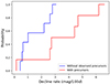 |
Fig. 10. Cumulative distributions of the rates of decline of the SNe IIn in our sample with (red) and without (blue) observed precursor activity. The two distributions are clearly separated, with SNe that showed precursor events declining faster after the explosion. |
In contrast, some SNe IIn remained luminous for years, being powered by continuous interaction with the CSM (such as SNe 2005ip, 2006jd, 2010jl, 2015da, and 2017hcc; Stritzinger et al. 2012; Ofek et al. 2019; Tartaglia et al. 2020; Moran et al. 2023). Two of those long-lasting events (SNe 2010jl and 2015da) are also part of our sample, and we did not see precursor activity prior to them. It is possible that the massive CSM necessary to sustain the SN for many years was produced decades before explosion, and is therefore missing from our data.
We mention a couple of caveats concerning the possible connection between the occurrence of precursors and the rates of decline of the SN light curves:
-
SNe without an observed precursor may also have experienced such events, with these remaining undetected in our data. This is especially true for the older SNe and for those for which we have few pre-explosion images.
-
A connection between the occurrence of pre-SN outbursts and the rates of decline of the SN light curves would not necessarily imply that these two phenomena are causally connected.
5.3. Occurrence rate of pre-SN outbursts
In contrast with previous works (O14, B15, S21), our investigation of pre-SN variability is not based on data regularly collected by a cadenced survey, as in PTF, KAIT/LOSS, and ZTF, but rather on images from both major surveys and observatory archives, whose temporal cadence is often random. This latter factor makes it impossible to obtain statistically robust quantitative estimations of the intrinsic pre-SN outburst occurrence rate and/or duration. Nevertheless, it is interesting to calculate a first-order estimation of the precursor event statistics from the data. As reported in Table 1, we detect precursor activity for 7 of the 27 SN IIn belonging to our sample. Nevertheless, as pointed out in the footnotes of Table 1, two events (SN 2011A and PTF11qnf) are considered as SN impostors (de Jaeger et al. 2015; Nyholm et al. 2017), while we suspect that SN 2018lkg is not a SN event (Appendix A). Thus, if we remove those three objects from our list of bona fide SNe IIn, the size of our sample shrinks to 24, while the number of SNe with precursors is unchanged (7, for a fraction of 29%). To decipher how the latter fraction compares with the intrinsic pre-SN outbursts occurrence rate, first of all, we need to obtain an estimation of the time during which we have images deep enough to detect a given precursor; we refer to this as our “control time (tc)”. To estimate tc for each SN, we ran a simulation17 that moves the maximum epoch of the Gaussian function through steps of one day across the time spanned between the earliest observation and the latest observation prior to the SN explosion. We then count the number of days during which at least one data point in the R, r, or Clear filters is beneath the function, or – in other words – during which the limiting flux of a certain observation is smaller than the expected flux of the function. As a consequence, if one upper limit is below the function with a certain maximum epoch, we would have spotted the outburst. The choice of the filters is dictated by the fact that most of the data are available in those filters. A visual representation of how the simulation works is shown in Fig. 11. With the same procedure, we also estimate another parameter that is important for our analysis, which is the duration of precursor activity (td). In this case, the days are counted when at least one precursor detection is beneath the Gaussian function. With this approach, we do not distinguish whether the points correspond to one long outburst or multiple short ones. As both the estimates of tc and td depend on the amplitude (ap) and the width (σp) of the Gaussians, we constructed a grid of ap and σp where the range of ap is from −11.5 to −15 mag (which are the faintest and brightest r-band absolute magnitudes of the detected precursor events), with steps of 0.5 mag. The range of σp is from 5 to 50 days (approximately the smallest and largest σp of the Gaussian fits to our precursors), with steps of 5 days. It is worth noting that changing the assumed value of the background level has a negligible effect on those calculations, because it is one order of magnitude lower than the amplitudes of the Gaussian derived from fitting the precursors. We then sum the td and tc times for all SNe in the sample for a specific ap and σp and calculate the ratio td/tc, which is plotted in Fig. 12. The median ratio is 0.22, with minimum and maximum values of 0.15 and 0.30, respectively. The overarching pattern indicates that the ratio smoothly increases with both the amplitude and the sigma of the Gaussian. Nevertheless, there is a significant increase in the ratio for ap of lower than −12.0, which is due to the fact that, in this range of flux, the contribution to both tc and td from the images retrieved by the DES survey starts to be relevant. The values of td/tc give us a first indication that the fraction of SN IIn for which we detect precursor activity in our sample is probably an underestimation of the real occurrence rate of pre-SN outbursts. Another, related insight can be obtained considering that the average tc18 for the SNe with detected precursor is 474 days, while the same quantity for the SNe without a detected precursor is 179 days. With a similar tc for both groups, we would also have a higher probability of detecting a precursor in SNe for which no activity was observed from our dataset. We note that if we remove SN 2016ehw – whose tc is 1054 days – from the subsample of SNe without precursors, the previously mentioned average tc value shrinks further to 120 days. On the other hand, the case of SN 2016ehw can be taken as an indication that probably not all SNe IIn display precursor activity before explosion. In addition to the monitoring time, the absolute flux limit that the images can probe has a strong impact on the precursor statistics. In this regard, if we only compute td/tc for the images obtained by DES survey, the ratio increases to 0.76, and we detect outbursts in two of the three SNe monitored as part of that survey. Finally, considering the strong assumption we make to compute td and tc – namely that all the progenitor outbursts have the same evolution represented by a Gaussian function–, we must warn the reader that all the above reported values have to be taken as order-of-magnitude estimations.
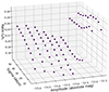 |
Fig. 11. Visualisation of the simulation used to estimate the rate of pre-SN precursors. The red triangles mark the upper limits (non-detections) of the prediscovery images of a SN in the sample, converted into solar luminosities. The blue curve is a Gaussian with ap = −14.5 r-band absolute magnitudes and σp = 20 days, while the green curve is a smaller one with ap = −12.5 mag and σp = 10 days. The quiescent luminosity of the progenitor is set at 1 × 10⁶ L⊙, and is shown by the grey dashed line. |
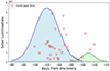 |
Fig. 12. Three-dimensional plot of the td/tc ratio calculated for a grid of parameters of the Gaussian functions. The ap ranges from −11.5 to −15 r-band absolute magnitudes with steps of 0.5 mag, while σp ranges from 5 to 50 days with steps of 5 days. The td/tc ratios have a median of 0.22, with a maximum of 0.30 and a minimum of 0.15. |
6. Conclusions
We searched for evidence of eruptive phases before the explosion of nearby SNe IIn. We constructed a sample of 27 SNe IIn situated within a DM of 34 mag, sufficiently close for modern high-cadence surveys searching for new transients to be able to detect events with an absolute magnitude of equal to or brighter that −14 mag. We looked at archival images of the SNe sites taken in the years prior to their discovery, both from the surveys and the public archives of major astronomical observatories. Among the 27 objects, at least 7 show robust signatures of one or more eruptive episodes, indicating that the progenitors were experiencing strong variability. As expected (Smith et al. 2011), the absolute magnitudes of these outbursts are between −11 and −15 mag, and the typical duration is a few weeks to months.
We constructed g − r colour curves of the outbursts with multi-band observations. The g − r colours of the outbursts are red, in the range of 0.5–1.0 mag. This is similar to the colour of LBVs during a giant eruption, when their atmospheres cool down and their spectra match those of F-type stars (Humphreys & Davidson 1994). However, this colour could also be an effect of strong Hα emission, a typical feature of SN impostors. We verified with spectra of SN impostor events that this effect can only partly explain the observed red colours, and therefore the major contribution comes from the cooler photospheric temperature.
To test whether the precursor activity had an effect on the post-explosion evolution, we measured the rates of decline of the light curves of the SNe after maximum light from publicly available data. The cumulative distributions of the SNe IIn with and without precursor activity show a marginal statistical difference, but contrary to expectations, the SNe that showed pre-explosion outbursts display much faster rates of decline, indicating that the pre-explosion activity does not have a significant effect on the SN IIn light curve. The latter finding is in line with the results obtained by O14 and S21.
Finally, we estimated the rate of the precursor events. We detect precursor activity in 29% of the bona fide SNe IIn in our sample, which confirms that Type IIn is a class of SN that frequently shows pre-explosion activity, in contrast with other SN types. Our estimation of the ratio between the time during which we detected activity and the time we could have detected activity provides an indication that the intrinsic occurrence rate of precursor events in the years prior to the terminal explosion is higher than that we obtain directly from the data; some activity may have been missed because of incomplete data or because of the lack of sensitivity of the instruments providing the data used here.
When the Legacy Survey in Space and Time at the Vera Rubin Observatory starts operations, it will scan the entire southern sky every two to three nights, reaching the 24th magnitude in a single 30 s exposure (Ivezić et al. 2019). It will be able to detect much fainter outbursts from the progenitors of close-by SNe IIn, and will detect the brightest events at much larger distances. In both cases, it will enlarge the number of SNe with observed precursor activity by orders of magnitude.
https://www.darkenergysurvey.org/
https://www.wis-tns.org/
https://wiserep.weizmann.ac.il/
http://graspa.oapd.inaf.it/asnc.html
https://atlas.fallingstar.com/
SNOoPy is a package for SN photometry using PSF fitting and/or template subtraction developed by E. Cappellaro at the Padova Astronomical Observatory. A package description can be found at http://sngroup.oapd.inaf.it/snoopy.html.
https://outerspace.stsci.edu/display/PANSTARRS/
https://www.aavso.org/apass
In these experiments, a fake star with the same magnitude and profile as the fitted source is placed in the template-subtracted image at a position close to but not coincident with the SN position. The magnitude of the fake star in the artificial image is then measured using the procedures described above. The dispersion of different measurements obtained from a number of iterations – with the artificial stars placed in slightly different positions – is then taken as an estimate of the instrumental magnitude error.
https://ps1images.stsci.edu/cgi-bin/ps1cutouts
https://irsa.ipac.caltech.edu/applications/ptf/
https://irsa.ipac.caltech.edu/applications/ztf/
https://sngroup.oapd.inaf.it/gap.html
https://ned.ipac.caltech.edu/
http://gsaweb.ast.cam.ac.uk/alerts/home
The Python code used to run the simulation with the Gaussians can be retrieved from Github: https://github.com/Astronomo94/ Gaussian-simulation
Using an average Gaussian with ap = −13.5 mag and σp = 15 days.
Acknowledgments
We thank the anonymous referee for their useful comments and suggestions, which improved the readability of the manuscript. A.R. acknowledges financial support from the GRAWITA Large Program Grant (PI P. D’Avanzo). A.P. and A.R. acknowledge the PRIN-INAF 2022 “Shedding light on the nature of gap transients: from the observations to the models”. R.D. acknowledges funds by ANID grant FONDECYT Postdoctorado N° 3220449. PTF was a scientific collaboration among the California Institute of Technology, Columbia University, Las Cumbres Observatory, the Lawrence Berkeley National Laboratory, the National Energy Research Scientific Computing Center, the University of Oxford, and the Weizmann Institute of Science. ZTF is supported by the National Science Foundation and a collaboration including Caltech, IPAC, the Weizmann Institute for Science, the Oskar Klein Center at Stockholm University, the University of Maryland, Deutsches Elektronen-Synchrotron and Humboldt University, Lawrence Livermore National Laboratory, the TANGO Consortium of Taiwan, the University of Wisconsin at Milwaukee, Trinity College Dublin, and Institut national de physique nucléaire et de physique des particules. Operations are conducted by COO, IPAC and University of Washington. Support for G.P. is provided by the Ministry of Economy, Development, and Tourism’s Millennium Science Initiative through grant IC120009, awarded to The Millennium Institute of Astrophysics (MAS). This research has made use of the NASA/IPAC Extragalactic Database (NED) which is operated by the Jet Propulsion Laboratory at the California Institute of Technology, under contract with the National Aeronautics and Space Administration. We acknowledge ESA Gaia, DPAC and the Photometric Science Alerts Team (http://gsaweb.ast.cam.ac.uk/alerts).
References
- Abbott, T. M. C., Abdalla, F. B., Allam, S., et al. 2018, ApJS, 239, 18 [Google Scholar]
- Arnett, W. D., & Meakin, C. 2011, ApJ, 741, 33 [NASA ADS] [CrossRef] [Google Scholar]
- Barbon, R., Cappellaro, E., & Turatto, M. 1989, A&AS, 81, 421 [NASA ADS] [Google Scholar]
- Barbon, R., Buondí, V., Cappellaro, E., & Turatto, M. 1999, A&AS, 139, 531 [NASA ADS] [CrossRef] [EDP Sciences] [Google Scholar]
- Bellm, E. C., Kulkarni, S. R., Graham, M. J., et al. 2019, PASP, 131, 018002 [Google Scholar]
- Bersier, D., Smartt, S., & Yaron, O. 2016, TNS Classif. Rep., 2016-650, 1 [Google Scholar]
- Bilinski, C., Smith, N., Li, W., et al. 2015, MNRAS, 450, 246 [NASA ADS] [CrossRef] [Google Scholar]
- Brennan, S. J., Elias-Rosa, N., Fraser, M., Van Dyk, S. D., & Lyman, J. D. 2022a, A&A, 664, L18 [NASA ADS] [CrossRef] [EDP Sciences] [Google Scholar]
- Brennan, S. J., Fraser, M., Johansson, J., et al. 2022b, MNRAS, 513, 5642 [NASA ADS] [Google Scholar]
- Brimacombe, J., & Holoien, T. 2016, TNSTR, 2016-123, 1 [NASA ADS] [Google Scholar]
- Brimacombe, J., Brown, J. S., Stanek, K. Z., et al. 2016, ATel, 9439, 1 [NASA ADS] [Google Scholar]
- Brown, J. S., Prieto, J. L., Shappee, B. J., et al. 2016, ATel, 9445, 1 [NASA ADS] [Google Scholar]
- Bruch, R. J., Gal-Yam, A., Schulze, S., et al. 2021, ApJ, 912, 46 [NASA ADS] [CrossRef] [Google Scholar]
- Cai, Y., Reguitti, A., Valerin, G., & Wang, X. 2022, Universe, 8, 493 [NASA ADS] [CrossRef] [Google Scholar]
- Campagnolo, J. C. N., Borges Fernandes, M., Drake, N. A., et al. 2018, A&A, 613, A33 [NASA ADS] [CrossRef] [EDP Sciences] [Google Scholar]
- Cappellaro, E. 2014, SNOoPY: A Package for SN Photometry https://sngroup.oapd.inaf.it/foscgui.html [Google Scholar]
- Cardelli, J. A., Clayton, G. C., & Mathis, J. S. 1989, ApJ, 345, 245 [Google Scholar]
- Chambers, K. C., Magnier, E. A., Metcalfe, N., et al. 2016, ArXiv e-prints [arXiv:1612.05560] [Google Scholar]
- Chambers, K. C., Boer, T. D., Bulger, J., et al. 2019, TNSTR, 2019-796, 1 [NASA ADS] [Google Scholar]
- Chevalier, R. A., & Fransson, C. 1994, ApJ, 420, 268 [NASA ADS] [CrossRef] [Google Scholar]
- Chugai, N. N., Chevalier, R. A., & Lundqvist, P. 2004, MNRAS, 355, 627 [CrossRef] [Google Scholar]
- de Jaeger, T., Anderson, J. P., Pignata, G., et al. 2015, ApJ, 807, 63 [NASA ADS] [CrossRef] [Google Scholar]
- Elias-Rosa, N., Pastorello, A., Benetti, S., et al. 2016, MNRAS, 463, 3894 [NASA ADS] [CrossRef] [Google Scholar]
- Elias-Rosa, N., Benetti, S., Cappellaro, E., et al. 2018, MNRAS, 475, 2614 [NASA ADS] [CrossRef] [Google Scholar]
- Filippenko, A. V. 1997, ARA&A, 35, 309 [NASA ADS] [CrossRef] [Google Scholar]
- Filippenko, A. V., Li, W. D., Treffers, R. R., & Modjaz, M. 2001, ASP Conf. Ser., 246, 121 [NASA ADS] [Google Scholar]
- Foley, R. J., Berger, E., Fox, O., et al. 2011, ApJ, 732, 32 [NASA ADS] [CrossRef] [Google Scholar]
- Förster, F., Cabrera-Vives, G., Castillo-Navarrete, E., et al. 2021, AJ, 161, 242 [CrossRef] [Google Scholar]
- Fransson, C., Sollerman, J., Strotjohann, N. L., et al. 2022, A&A, 666, A79 [NASA ADS] [CrossRef] [EDP Sciences] [Google Scholar]
- Fraser, M. 2020, R. Soc. Open Sci., 7, 200467 [NASA ADS] [CrossRef] [Google Scholar]
- Fraser, M., Magee, M., Kotak, R., et al. 2013, ApJ, 779, L8 [NASA ADS] [CrossRef] [Google Scholar]
- Fremling, C., Dugas, A., & Sharma, Y. 2019, TNS Classif. Rep., 2019-747, 1 [Google Scholar]
- Fuller, J. 2017, MNRAS, 470, 1642 [NASA ADS] [CrossRef] [Google Scholar]
- Fuller, J., & Ro, S. 2018, MNRAS, 476, 1853 [NASA ADS] [CrossRef] [Google Scholar]
- Gal-Yam, A., & Leonard, D. C. 2009, Nature, 458, 865 [NASA ADS] [CrossRef] [Google Scholar]
- Gal-Yam, A., Leonard, D. C., Fox, D. B., et al. 2007, ApJ, 656, 372 [NASA ADS] [CrossRef] [Google Scholar]
- Gal-Yam, A., Arcavi, I., Ofek, E. O., et al. 2014, Nature, 509, 471 [CrossRef] [Google Scholar]
- Graham, M. L., Sand, D. J., Valenti, S., et al. 2014, ApJ, 787, 163 [NASA ADS] [CrossRef] [Google Scholar]
- Graham, M. L., Dahiwale, A., & Fremling, C. 2020, TNS Classif. Rep., 2020-603, 1 [Google Scholar]
- Humphreys, R. M., & Davidson, K. 1994, PASP, 106, 1025 [NASA ADS] [CrossRef] [Google Scholar]
- Ivezić, Ž., Kahn, S. M., Tyson, J. A., et al. 2019, ApJ, 873, 111 [Google Scholar]
- Jacobson-Galán, W. V., Dessart, L., Jones, D. O., et al. 2022, ApJ, 924, 15 [CrossRef] [Google Scholar]
- Jencson, J. E., Sand, D. J., Andrews, J. E., et al. 2022, ApJ, 935, L33 [CrossRef] [Google Scholar]
- Jester, S., Schneider, D. P., Richards, G. T., et al. 2005, AJ, 130, 873 [Google Scholar]
- Kasliwal, M. M. 2012, PASA, 29, 482 [NASA ADS] [CrossRef] [Google Scholar]
- Law, N. M., Kulkarni, S. R., Dekany, R. G., et al. 2009, PASP, 121, 1395 [NASA ADS] [CrossRef] [Google Scholar]
- Margutti, R., Milisavljevic, D., Soderberg, A. M., et al. 2014, ApJ, 780, 21 [Google Scholar]
- Masci, F. J., Laher, R. R., Rusholme, B., et al. 2019, PASP, 131, 018003 [Google Scholar]
- Mattila, S., Meikle, W. P. S., Lundqvist, P., et al. 2008, MNRAS, 389, 141 [NASA ADS] [CrossRef] [Google Scholar]
- Mauerhan, J. C., Smith, N., Filippenko, A. V., et al. 2013a, MNRAS, 430, 1801 [NASA ADS] [CrossRef] [Google Scholar]
- Mauerhan, J. C., Smith, N., Silverman, J. M., et al. 2013b, MNRAS, 431, 2599 [Google Scholar]
- Monard, L. A. G., Prieto, J. L., & Seth, K. 2011, CBETs, 2799, 1 [NASA ADS] [Google Scholar]
- Moran, S., Fraser, M., Kotak, R., et al. 2023, A&A, 669, A51 [NASA ADS] [CrossRef] [EDP Sciences] [Google Scholar]
- Moriya, T. J., Galbany, L., Jiménez-Palau, C., et al. 2023, A&A, 677, A20 [NASA ADS] [CrossRef] [EDP Sciences] [Google Scholar]
- Nordin, J., Brinnel, V., Giomi, M., et al. 2019, TNSTR, 2019-404, 1 [NASA ADS] [Google Scholar]
- Nyholm, A., Sollerman, J., Taddia, F., et al. 2017, A&A, 605, A6 [NASA ADS] [CrossRef] [EDP Sciences] [Google Scholar]
- Ofek, E. O., Sullivan, M., Cenko, S. B., et al. 2013, Nature, 494, 65 [CrossRef] [Google Scholar]
- Ofek, E. O., Sullivan, M., Shaviv, N. J., et al. 2014, ApJ, 789, 104 [NASA ADS] [CrossRef] [Google Scholar]
- Ofek, E. O., Zackay, B., Gal-Yam, A., et al. 2019, PASP, 131, 054204 [NASA ADS] [CrossRef] [Google Scholar]
- Pan, Y. C., Foley, R. J., Jha, S. W., Rest, A., & Scolnic, D. 2016, ATel, 9129, 1 [NASA ADS] [Google Scholar]
- Parker, S. 2016, TNSTR, 2016-422, 1 [NASA ADS] [Google Scholar]
- Pastorello, A., & Fraser, M. 2019, Nat. Astron., 3, 676 [Google Scholar]
- Pastorello, A., Quimby, R. M., Smartt, S. J., et al. 2008, MNRAS, 389, 131 [NASA ADS] [CrossRef] [Google Scholar]
- Pastorello, A., Botticella, M. T., Trundle, C., et al. 2010, MNRAS, 408, 181 [NASA ADS] [CrossRef] [Google Scholar]
- Pastorello, A., Cappellaro, E., Inserra, C., et al. 2013, ApJ, 767, 1 [NASA ADS] [CrossRef] [Google Scholar]
- Pastorello, A., Kochanek, C. S., Fraser, M., et al. 2018, MNRAS, 474, 197 [NASA ADS] [CrossRef] [Google Scholar]
- Pastorello, A., Reguitti, A., Morales-Garoffolo, A., et al. 2019, A&A, 628, A93 [NASA ADS] [CrossRef] [EDP Sciences] [Google Scholar]
- Pessi, T., Prieto, J. L., Monard, B., et al. 2022, ApJ, 928, 138 [NASA ADS] [CrossRef] [Google Scholar]
- Pignata, G., Maza, J., Antezana, R., et al. 2009, AIP Conf. Ser., 1111, 551 [NASA ADS] [CrossRef] [Google Scholar]
- Pozzo, M., Meikle, W. P. S., Fassia, A., et al. 2004, MNRAS, 352, 457 [CrossRef] [Google Scholar]
- Quataert, E., & Shiode, J. 2012, MNRAS, 423, L92 [NASA ADS] [CrossRef] [Google Scholar]
- Ransome, C. L., Habergham-Mawson, S. M., Darnley, M. J., et al. 2021, MNRAS, 506, 4715 [NASA ADS] [CrossRef] [Google Scholar]
- Reguitti, A., Pastorello, A., Pignata, G., et al. 2019, MNRAS, 482, 2750 [NASA ADS] [Google Scholar]
- Reguitti, A., Pastorello, A., Pignata, G., et al. 2022, A&A, 662, L10 [NASA ADS] [CrossRef] [EDP Sciences] [Google Scholar]
- Reichart, D., Nysewander, M., Moran, J., et al. 2005, Space Phys. C, 28, 767 [NASA ADS] [Google Scholar]
- Rodríguez, Ó., Pignata, G., Anderson, J. P., et al. 2020, MNRAS, 494, 5882 [CrossRef] [Google Scholar]
- Schlafly, E. F., & Finkbeiner, D. P. 2011, ApJ, 737, 103 [Google Scholar]
- Schlegel, E. M. 1990, MNRAS, 244, 269 [NASA ADS] [Google Scholar]
- Shappee, B., Prieto, J., Stanek, K. Z., et al. 2014, Am. Astron. Soc. Meet. Abstr., 223, 236.03 [Google Scholar]
- Shiode, J. H., & Quataert, E. 2014, ApJ, 780, 96 [Google Scholar]
- Smartt, S. J., Valenti, S., Fraser, M., et al. 2015, A&A, 579, A40 [NASA ADS] [CrossRef] [EDP Sciences] [Google Scholar]
- Smith, N. 2017, in Handbook of Supernovae, eds. A. W. Alsabti, & P. Murdin (Springer International Publishing AG), 403 [Google Scholar]
- Smith, N., & Arnett, W. D. 2014, ApJ, 785, 82 [NASA ADS] [CrossRef] [Google Scholar]
- Smith, N., Foley, R. J., & Filippenko, A. V. 2008, ApJ, 680, 568 [Google Scholar]
- Smith, N., Miller, A., Li, W., et al. 2010, AJ, 139, 1451 [NASA ADS] [CrossRef] [Google Scholar]
- Smith, N., Li, W., Silverman, J. M., Ganeshalingam, M., & Filippenko, A. V. 2011, MNRAS, 415, 773 [NASA ADS] [CrossRef] [Google Scholar]
- Smith, N., Cenko, S. B., Butler, N., et al. 2012, MNRAS, 420, 1135 [NASA ADS] [CrossRef] [Google Scholar]
- Smith, N., Mauerhan, J. C., & Prieto, J. L. 2014, MNRAS, 438, 1191 [NASA ADS] [CrossRef] [Google Scholar]
- Smith, N., Andrews, J. E., Filippenko, A. V., et al. 2022, MNRAS, 515, 71 [NASA ADS] [CrossRef] [Google Scholar]
- Stritzinger, M., Taddia, F., Fransson, C., et al. 2012, ApJ, 756, 173 [NASA ADS] [CrossRef] [Google Scholar]
- Strotjohann, N. L., Ofek, E. O., Gal-Yam, A., et al. 2021, ApJ, 907, 99 [NASA ADS] [CrossRef] [Google Scholar]
- Taddia, F., Stritzinger, M. D., Sollerman, J., et al. 2013, A&A, 555, A10 [NASA ADS] [CrossRef] [EDP Sciences] [Google Scholar]
- Tartaglia, L., Pastorello, A., Taubenberger, S., et al. 2015, MNRAS, 447, 117 [NASA ADS] [CrossRef] [Google Scholar]
- Tartaglia, L., Pastorello, A., Sullivan, M., et al. 2016, MNRAS, 459, 1039 [NASA ADS] [CrossRef] [Google Scholar]
- Tartaglia, L., Pastorello, A., Sollerman, J., et al. 2020, A&A, 635, A39 [NASA ADS] [CrossRef] [EDP Sciences] [Google Scholar]
- Taubenberger, S., Faran, T., Kromer, M., Elias-rosa, N., & Yaron, O. 2016, TNS Classif. Rep., 2016-150, 1 [Google Scholar]
- Thöne, C. C., de Ugarte Postigo, A., Leloudas, G., et al. 2017, A&A, 599, A129 [NASA ADS] [CrossRef] [EDP Sciences] [Google Scholar]
- Tonry, J. L., Denneau, L., Heinze, A. N., et al. 2018, PASP, 130, 064505 [Google Scholar]
- Tsvetkov, D. Y., Pavlyuk, N., Karnaukhov, P., et al. 2020, Peremennye Zvezdy, 40, 4 [NASA ADS] [Google Scholar]
- Van Dyk, S. D., Peng, C. Y., King, J. Y., et al. 2000, PASP, 112, 1532 [NASA ADS] [CrossRef] [Google Scholar]
- Wagner, R. M., Vrba, F. J., Henden, A. A., et al. 2004, PASP, 116, 326 [CrossRef] [Google Scholar]
- Woosley, S. E., Blinnikov, S., & Heger, A. 2007, Nature, 450, 390 [NASA ADS] [CrossRef] [PubMed] [Google Scholar]
- Wu, S., & Fuller, J. 2021, ApJ, 906, 3 [NASA ADS] [CrossRef] [Google Scholar]
- Wu, S. C., & Fuller, J. 2022, ApJ, 930, 119 [NASA ADS] [CrossRef] [Google Scholar]
- Yaron, O., & Gal-Yam, A. 2012, PASP, 124, 668 [Google Scholar]
- Zhang, T., Wang, X., Wu, C., et al. 2012, AJ, 144, 131 [NASA ADS] [CrossRef] [Google Scholar]
- Zhang, X., Xiang, D., Lin, H., et al. 2019, ATel, 12358, 1 [NASA ADS] [Google Scholar]
Appendix A: SN (AT) 2018lkg
Analysing the sample, we note that SN 2018lkg is possibly an active galactic nucleus, or a tidal disruption event, rather than a Type IIn SN, because the transient sits in the centre of its host galaxy, and the multiple outbursts are unreasonably luminous to be produced by non-terminal stellar eruptions (being at nearly Mr ∼ −16 mag; see Fig. A.1). Furthermore, the classification spectrum (Zhang et al. 2019) reveals broad H features instead of the classical narrow lines of SNe IIn.
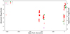 |
Fig. A.1. Prediscovery gr light curve of SN 2018lkg. In 2013, PTF detected a precursor event with an absolute Mr of −16 mag, which is brighter than typical non-terminal events. |
Appendix B: Table of Observatories archives
Observatory locations and telescopes for which we consulted the public archives searching for pre-explosion images of SNe IIn. The observatories in the second part of the table do not provide additional useful images.
All Tables
Observatory locations and telescopes for which we consulted the public archives searching for pre-explosion images of SNe IIn. The observatories in the second part of the table do not provide additional useful images.
All Figures
|
Fig. 1. Pre- and post-discovery observation of SN 2011fh. Clear filter magnitudes from the CHASE Survey and from amateurs are plotted as V-band, a single w-band LCOGT observation as R-band, and the 2016 HST F814W observation as I-band. Observations from different instruments are plotted with different symbols. The late-time luminosity level is marked with a dashed line. A zoom onto the rise to the 2011 event is plotted in the inset window, showing the first year of decline, during which a second, smaller peak is visible at +250 days. |
| In the text | |
|
Fig. 2. Spectrum of SN 2011fh taken with the 6.5 m Clay telescope+LDSS3 12 yr after maximum light. The principal identified emission lines are marked. |
| In the text | |
|
Fig. 3. Pre-discovery griz observations of SN 2016aiy from the DES survey. The phases are relative to the V-band maximum (Reguitti et al., in prep.). |
| In the text | |
|
Fig. 4. Pre-discovery light curves of SN 2016cvk. The clear filter observations from the CHASE are in blue, and the other points are with Sloan filters from the DECam instrument. The open inverted triangles are upper limits, and the filled circles are detections. The larger triangles with a horizontal error bar indicate more profound upper limits derived from stacked frames within the temporal bar. The phases are relative to the V-band maximum (Matilainen et al., in prep.). |
| In the text | |
|
Fig. 5. Pre- and post-explosion light curves of SN 2019bxq. Top: Pre-explosion R-band absolute light curve of SN 2019bxq from the PTF survey. The data span the 2009–2011 period. The magnitudes are corrected for the adopted distance modulus and Galactic reddening. The phase on the x-axis is from the SN r-band maximum (MJD = 58577). The open inverted triangles mark upper limits (i.e. non-detections). Bottom left: Same as above, but including all the available data (PTF+ZTF+sparse archive data). Observations from different instruments are plotted with different symbols. The phases are relative to the brightest r-band point in the SN light curve. Bottom right: Post-explosion g- and r-band light curves of SN 2019bxq from the ZTF survey. The SN light curves are shown to highlight the short duration of the SN event. |
| In the text | |
|
Fig. 6. Pre- and post-explosion light curves of SN 2019fmb. Left: Pre- and post-discovery (MJD = 58 615) Sloan-gri detections from the ZTF and PS-1 surveys of SN 2019fmb. Observations from different instruments are plotted with different symbols. The phases are relative to the brightest r-band point in the SN light curve. The deepest upper limits of the object in g-, r- and z-band filters from NOAO archival data of 2016 are marked with horizontal lines in the bottom-left corner. Right: Light curve of SN 2019fmb, with the detections by ATLAS also reported. As for SN 2019bxq, the SN has a short duration. |
| In the text | |
|
Fig. 7. Gaussian fit (dashed line) over the r-band light curve of the pre-SN outburst before SN 2019fmb. The magnitudes of the data points were converted into fluxes, and then normalised with respect to the peak of the Gaussian fit and centred on the epoch of the maximum. |
| In the text | |
|
Fig. 8. g − r colour of the three pre-SN outbursts or activities for which multi-band photometry is available. The phases are relative to the maximum in the r-band, which was derived from a Gaussian fit over the data points. For comparison, the V − R colour of the 2000 and 2008 outbursts of the known LBV AT 2000ch (Pastorello et al. 2010) and of the SN impostor SN 2007sv (Tartaglia et al. 2015) are also shown. The g − r colour of the outbursts is red, around g − r∼0.5 mag. |
| In the text | |
|
Fig. 9. Histogram of the distribution of the difference in the r-band synthetic photometry – with and without the Hα contribution – of the classification spectra for a sample of SN impostors and LBV eruptions. |
| In the text | |
|
Fig. 10. Cumulative distributions of the rates of decline of the SNe IIn in our sample with (red) and without (blue) observed precursor activity. The two distributions are clearly separated, with SNe that showed precursor events declining faster after the explosion. |
| In the text | |
|
Fig. 11. Visualisation of the simulation used to estimate the rate of pre-SN precursors. The red triangles mark the upper limits (non-detections) of the prediscovery images of a SN in the sample, converted into solar luminosities. The blue curve is a Gaussian with ap = −14.5 r-band absolute magnitudes and σp = 20 days, while the green curve is a smaller one with ap = −12.5 mag and σp = 10 days. The quiescent luminosity of the progenitor is set at 1 × 10⁶ L⊙, and is shown by the grey dashed line. |
| In the text | |
|
Fig. 12. Three-dimensional plot of the td/tc ratio calculated for a grid of parameters of the Gaussian functions. The ap ranges from −11.5 to −15 r-band absolute magnitudes with steps of 0.5 mag, while σp ranges from 5 to 50 days with steps of 5 days. The td/tc ratios have a median of 0.22, with a maximum of 0.30 and a minimum of 0.15. |
| In the text | |
|
Fig. A.1. Prediscovery gr light curve of SN 2018lkg. In 2013, PTF detected a precursor event with an absolute Mr of −16 mag, which is brighter than typical non-terminal events. |
| In the text | |
Current usage metrics show cumulative count of Article Views (full-text article views including HTML views, PDF and ePub downloads, according to the available data) and Abstracts Views on Vision4Press platform.
Data correspond to usage on the plateform after 2015. The current usage metrics is available 48-96 hours after online publication and is updated daily on week days.
Initial download of the metrics may take a while.