| Issue |
A&A
Volume 599, March 2017
|
|
|---|---|---|
| Article Number | A142 | |
| Number of page(s) | 27 | |
| Section | Atomic, molecular, and nuclear data | |
| DOI | https://doi.org/10.1051/0004-6361/201629794 | |
| Published online | 16 March 2017 | |
Stellar laboratories
VIII. New Zr iv–vii, Xe iv–v, and Xe vii oscillator strengths and the Al, Zr, and Xe abundances in the hot white dwarfs G191−B2B and RE 0503−289⋆,⋆⋆,⋆⋆⋆
1 Institute for Astronomy and Astrophysics, Kepler Center for Astro and Particle Physics, Eberhard Karls University, Sand 1, 72076 Tübingen, Germany
e-mail: This email address is being protected from spambots. You need JavaScript enabled to view it.
2 Physique Atomique et Astrophysique, Université de Mons – UMONS, 7000 Mons, Belgium
3 IPNAS, Université de Liège, Sart Tilman, 4000 Liège, Belgium
4 NASA Goddard Space Flight Center, Greenbelt, MD 20771, USA
5 Astronomisches Rechen-Institut (ARI), Centre for Astronomy of Heidelberg University, Mönchhofstraße 12–14, 69120 Heidelberg, Germany
Received: 27 September 2016
Accepted: 6 November 2016
Abstract
Context. For the spectral analysis of high-resolution and high-signal-to-noise spectra of hot stars, state-of-the-art non-local thermodynamic equilibrium (NLTE) model atmospheres are mandatory. These are strongly dependent on the reliability of the atomic data that is used for their calculation.
Aims. To search for zirconium and xenon lines in the ultraviolet (UV) spectra of G191−B2B and RE 0503−289, new Zr iv–vii, Xe iv–v, and Xe vii oscillator strengths were calculated. This allows, for the first time, determination of the Zr abundance in white dwarf (WD) stars and improvement of the Xe abundance determinations.
Methods. We calculated Zr iv–vii, Xe iv–v, and Xe vii oscillator strengths to consider radiative and collisional bound-bound transitions of Zr and Xe in our NLTE stellar-atmosphere models for the analysis of their lines exhibited in UV observations of the hot WDs G191−B2B and RE 0503−289.
Results. We identified one new Zr iv, 14 new Zr v, and ten new Zr vi lines in the spectrum of RE 0503−289. Zr was detected for the first time in a WD. We measured a Zr abundance of −3.5 ± 0.2 (logarithmic mass fraction, approx. 11 500 times solar). We identified five new Xe vi lines and determined a Xe abundance of −3.9 ± 0.2 (approx. 7500 times solar). We determined a preliminary photospheric Al abundance of −4.3 ± 0.2 (solar) in RE 0503−289. In the spectra of G191−B2B, no Zr line was identified. The strongest Zr iv line (1598.948 Å) in our model gave an upper limit of −5.6 ± 0.3 (approx. 100 times solar). No Xe line was identified in the UV spectrum of G191−B2B and we confirmed the previously determined upper limit of −6.8 ± 0.3 (ten times solar).
Conclusions. Precise measurements and calculations of atomic data are a prerequisite for advanced NLTE stellar-atmosphere modeling. Observed Zr iv–vi and Xe vi-vii line profiles in the UV spectrum of RE 0503−289 were simultaneously well reproduced with our newly calculated oscillator strengths.
Key words: atomic data / line: identification / stars: abundances / stars: individual: G191-B2B / stars: individual: RE0503-289 / virtual observatory tools
Based on observations with the NASA/ESA Hubble Space Telescope, obtained at the Space Telescope Science Institute, which is operated by the Association of Universities for Research in Astronomy, Inc., under NASA contract NAS5-26666.
Based on observations made with the NASA-CNES-CSA Far Ultraviolet Spectroscopic Explorer.
Tables A.9–A.12 and B.5–B.7 are only available via the German Astrophysical Virtual Observatory (GAVO) service TOSS (http://dc.g-vo.org/TOSS).
© ESO, 2017
1. Introduction
The DO-type white dwarf (WD) star RE 0503−289 (WD 0501+527, McCook & Sion 1999a,b), exhibits many lines of the trans-iron elements Zn (atomic number Z = 30), Ga (31), Ge (32), As (33), Se (34), Kr (36), Mo (42), Sn (50), Te (52), I (53), Xe (54), and Ba (56) in its ultraviolet spectrum. These were initially identified by Werner et al. (2012b), who determined the Kr and Xe abundances (Sect. 8) based on atomic data available at that time. Calculations of transition probabilities for Zn, Ga, Ge, Kr, Mo, Xe, and Ba in the subsequent years allowed precise abundance measurements for these elements (Rauch et al. 2014a, 2015b, 2012, 2016a, 2014b, 2015a, 2016b, respectively).
Here we report that we have identified lines of an additional element, namely zirconium (40) which has never been detected before in WDs, and calculated new Zr iv–vii transition probabilities to determine its photospheric abundance. To verify the Xe abundance determination of Werner et al. (2012b), we calculated much more complete Xe iv–v and Xe vi transition probabilities.
The hot, hydrogen-rich, DA-type WD G191−B2B (WD 0501+527, McCook & Sion 1999a,b) is a primary flux reference standard for all absolute calibrations from 1000 to 25 000 Å (Bohlin 2007). Rauch et al. (2013) presented a detailed spectral analysis of this star. Based on their model, Rauch et al. (2014a, 2015b, 2014b) identified Zn, Ga, and Ba lines in the observed UV spectrum and determined the abundances of these elements.
We briefly introduce our observational data in Sect. 2. The discovery of the interstellar Mg iiλλ 2796.35,2803.53 Å resonance doublet and its modelling is shown in Sect. 3. Our model atmospheres are described in Sect. 4. We start our spectral analysis with a search for Al lines and an abundance determination in Sect. 5. The Zr transition-probability calculation, line identification, and abundance analysis are presented in Sect. 6, followed by the same for Xe in Sect. 7. We summarize our results and conclude in Sect. 8.
2. Observations
For RE 0503−289, we analyzed ultraviolet (UV) observations that were obtained with the Far Ultraviolet Spectroscopic Explorer (FUSE, 910 Å < λ < 1188 Å, resolving power R = λ/ Δλ ≈ 20 000) and the Hubble Space Telescope/Space Telescope Imaging Spectrograph (HST/STIS, 1144 Å < λ < 3073 Å, R ≈ 45 800). These were described in detail by Werner et al. (2012b) and Rauch et al. (2016b), respectively.
For G191−B2B, we used the FUSE observation described by Rauch et al. (2013) and the high-dispersion échelle spectrum (HST/STIS, 1145−3145 Å, R ≈ 100 000, Rauch et al. 2013) available from the CALSPEC1 database.
Column densities (in cm-2) and radial velocities (in km s-1) used to model interstellar clouds in the line of sight toward RE 0503−289.
To compare observations with synthetic spectra, the latter were convolved with Gaussians to model the respective resolving power. The observed spectra are shifted to rest wavelengths according to radial-velocity measurements of vrad = 24.56 km s-1 (Lemoine et al. 2002) and 25.8 km s-1 for G191−B2B and RE 0503−289 (our value), respectively.
3. Interstellar line absorption
Rauch et al. (2016b) found that the interstellar line absorption toward RE 0503−289 has a multi-velocity structure (radial-velocities −40 km s-1 < vrad < + 18 km s-1). In the HST/STIS spectra of RE 0503−289, the interstellar Mg iiλλ 2796.35,2803.53 Å resonance lines (3s 2S1/2–3p 2P and 3s 2S1/2–3p 2P
 with oscillator strengths of 0.608 and 0.303, respectively) are prominent (Fig. 1) and corroborate such a structure. Table 1 displays the parameters that were used to fit the observation.
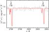 |
Fig. 1 Section of the STIS spectrum of RE 0503−289 with the interstellar Mg iiλλ 2796.35,2803.53 Å lines. |
4. Model atmospheres and atomic data
We calculated plane-parallel, chemically homogeneous model-atmospheres in hydrostatic and radiative equilibrium with the Tübingen non-local thermodynamic equilibrium (NLTE) Model Atmosphere Package (TMAP2, Werner et al. 2003, 2012a). Model atoms were retrieved from the Tübingen Model Atom Database (TMAD3, Rauch & Deetjen 2003) that has been constructed as part of the Tübingen contribution to the German Astrophysical Virtual Observatory (GAVO4).
The effective temperatures, surface gravities, and photospheric abundances of G191−B2B (Teff = 60 000 ± 2000 K, log (g/ cm s-2) = 7.6 ± 0.05, Rauch et al. 2013) and RE 0503−289 (Teff = 70 000 ± 2000 K, log g = 7.50 ± 0.1, Rauch et al. 2016b) were previously analyzed with TMAP models. We adopt these parameters for our calculations.
Zr iv–vii and Xe iv–vii were represented by the Zr and Xe model atoms with so-called super levels and super lines that were calculated with a statistical approach via our Iron Opacity and Interface (IrOnIc5, Rauch & Deetjen 2003; Müller-Ringat 2013). To enable IrOnIc to read our new Zr and Xe data, we transferred it into Kurucz-formatted files (cf., Rauch et al. 2015b). The statistics of our Zr and Xe model atoms is listed in Table 2.
Statistics of Zr iv–vii and Xe iv–v, vii atomic levels and line transitions from Tables A.9–A.12 and B.5–B.7, respectively.
For Zr and Xe and all other species, level dissolution (pressure ionization) following Hummer & Mihalas (1988) and Hubeny et al. (1994) is accounted for. Broadening for all Al, Zr, and Xe lines due to the quadratic Stark effect is calculated using approximate formulae given by Cowley (1970, 1971).
All spectral energy distributions (SEDs) that were calculated for this analysis are available via the registered Theoretical Stellar Spectra Access (TheoSSA6) GAVO service.
5. Aluminum in RE 0503−289
The Al abundance in RE 0503−289 was hitherto undetermined. TMAD provides a recently extended Al model atom (Table 3). We used it to search for Al lines in the UV and optical spectra of G191−B2B and RE 0503−289, especially for Al iv lines, because, in both stars, this is the dominant ionization stage in the line-forming region (−4 ≲ log m ≲ 0.5, Figs. 2, 3). So far, only Al iii lines were identified in the UV spectrum of G191−B2B, namely λλ1854.714,1862.787 Å (Holberg et al. 1998) and λλ1379.668,1384.130,1605.764,1611.812,1611.854 Å (Rauch et al. 2013, logarithmic mass fraction of Al =−4.95 ± 0.2).
Statistics of the Al model atom used in our calculations compared to our previous analyses (e.g., Rauch et al. 2013, 2016b).
The only additional Al lines found in the observed spectra of G191−B2B are Al III λλ 1935.840,1935.863,1935.949 Å (Fig. 4). Al iv lines in our model are entirely too weak to detect them in the observations. Compared to the available STIS spectrum of G191−B2B, that of RE 0503−289 has a much lower signal-to-noise ratio (S/N) that hampers detection of Al lines. Al III λλ 1384.130 Å is the only line that is present in the observation and is well reproduced at a solar Al abundance (−4.28 ± 0.2). This result is based on a single line only, and thus it must be judged as uncertain. It is, however, at least an upper abundance limit. The derived abundance is, nonetheless, in good agreement with the expectation (interpolation in Fig. 10). To improve the Al abundance measurement, better UV spectra for RE 0503−289 are highly desirable.
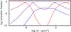 |
Fig. 2 Al ionization fractions in our G191−B2B model. m is the column mass, measured from the outer boundary of our model atmospheres. |
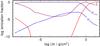 |
Fig. 3 As Fig. 2, for RE 0503−289. |
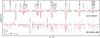 |
Fig. 4 Comparison of sections of the STIS spectra with our models for G191−B2B (top) and RE 0503−289 (bottom). The Al abundances are 1.1 × 10⁻⁵ (0.2 times the solar value, Rauch et al. 2013) and 5.3 × 10⁻⁵ (solar), respectively. In the top part, the green dashed line is a spectrum calculated without Al. Prominent lines are marked, the identified Al iii lines with their wavelengths. |
6. Zirconium
6.1. Oscillator-strength calculations for Zr IV–VII ions
Radiative decay rates (oscillator strengths and transition probabilities) were computed using the pseudo-relativistic Hartree-Fock (HFR) method originally introduced by Cowan (1981), and modified for taking into account core-polarization effects (CPOL), giving rise to the HFR+CPOL approach (e.g., Quinet et al. 1999, 2002).
For Zr iv, configuration interaction was considered among the configurations 4s24p6nd (n = 4–9), 4s24p6ns (n = 5–9), 4s24p6ng (n = 5–9), 4s24p6ni (n = 7–9), 4s24p54d5p, 4s24p54d4f, and 4s24p54d5f for the even parity, and 4s24p6np (n = 5–9), 4s24p6nf (n = 4–9), 4s24p6nh (n = 6–9), 4s24p6nk (n = 8–9), 4s24p54d2, 4s24p54d5s, and 4s24p54d5d for the odd parity. The core-polarization parameters were the dipole polarizability of a Zr vi ionic core as reported by Fraga et al. (1976), that is, αd = 2.50 a.u., and the cut-off radius corresponding to the HFR mean value ⟨ r ⟩ of the outermost core orbital (4p), that is, rc = 1.34 a.u. Using the experimental energy levels taken from the analysis by Reader & Acquista (1997), the average energies and spin-orbit parameters of 4s24p6nd (n = 4–6), 4s24p6ns (n = 5–8), 4s24p6ng (n = 5–9), 4s24p6np (n = 5–7), 4s24p6nf (n = 4–6), and 4s24p66h configurations were adjusted using a well-established least-squares fitting procedure in which the mean deviations with experimental data were found to be equal to 0 cm-1 for the even parity and 6 cm-1 for the odd parity.
For Zr v, the configurations explicitly included in the HFR model were 4s24p6, 4s24p5np (n = 5–7), 4s24p5nf (n = 4–7), 4s4p6nd (n = 4–7), 4s4p6ns (n = 5–7), 4s24p44d2, 4s24p44d5s, and 4s24p45s2 for the even parity, and 4s24p5nd (n = 4–7), 4s24p5ns (n = 5–10), 4s24p5ng (n = 5–7), 4s4p6np (n = 5–7), 4s4p6nf (n = 4–7), 4s24p44d5p, and 4s24p44d4f for the odd parity. Core-polarization effects were estimated using αd = 0.08 a.u. and rc = 0.45 a.u. These values correspond to a Ni-like Zr xiii ionic core, with 3d as an outermost core subshell. In this ion, the semi-empirical process was performed to optimize the average energies, spin-orbit parameters, and electrostatic interaction. Slater integrals corresponding to 4p6, 4p5np (n = 5–6), 4p54f, 4s4p64d, 4p5nd (n = 4–7), 4p5ns (n = 5–10), 4p5ng (n = 5–6), and 4s4p65p configurations using the experimental levels reported by Reader & Acquista (1979) and Khan et al. (1981). The mean deviations between calculated and experimental energies were 77 cm-1 and 91 cm-1 for even and odd parities, respectively.
In the case of Zr vi, the HFR method was used with the interacting configurations 4s24p5, 4s24p4np (n = 5–6), 4s24p4nf (n = 4–6), 4s4p5nd (n = 4–6), 4s4p5ns (n = 5–6), 4p6np (n = 5–6), 4p6nf (n = 4–6), 4s24p34d2, 4s24p34d5s, and 4s24p35s2 for the odd parity, and 4s4p6, 4s24p4nd (n = 4–6), 4s24p4ns (n = 5–6), 4s24p4ng (n = 5–6), 4s4p5np (n = 5–6), 4s4p5nf (n = 4–6), 4p6ns (n = 5–6), 4p6nd (n = 4–6), 4s24p34d5p, and 4s24p34d4f for the even parity. Core-polarization effects were estimated using the same αd and rc values as those considered in Zr v. The radial integrals corresponding to 4p5, 4p45p, 4s4p6, 4p45d, 4p45s, and 4p46s were adjusted to minimize the differences between the calculated Hamiltonian eigenvalues and the experimental energy levels taken from Reader & Lindsay (2016). In this process, we found mean deviations equal to 111 cm-1 in the odd parity and 221 cm-1 in the even parity.
Finally, for Zr vii, the configurations included in the HFR model were 4s24p4, 4s24p3np (n = 5–6), 4s24p3nf (n = 4–6), 4s4p4nd (n = 4–6), 4s4p4ns (n = 5–6), 4p5np (n = 5–6), 4p5nf (n = 4–6), 4s24p24d2, 4s24p24d5s, and 4s24p25s2 for the even parity, and 4s4p5, 4s24p3nd (n = 4–6), 4s24p3ns (n = 5–6), 4s24p3ng (n = 5–6), 4s4p4np (n = 5–6), 4s4p4nf (n = 4–6), 4p5ns (n = 5–6), 4p5nd (n = 4–6), 4s24p24d5p, and 4s24p24d4f for the odd parity. The same core-polarization parameters as those used in Zr v and Zr vi calculations were considered while the radial integrals of 4p4, 4p35p, 4s4p5, 4p34d, and 4p35s were optimized with the experimental energy levels taken from Reader & Acquista (1976), Rahimullah et al. (1978), Khan et al. (1983). Although having established level values, the 4p34f configuration was not fitted because it appeared very strongly mixed with experimentally unknown configurations such as 4s4p44d, and 4s24p24d2 according to our HFR calculations. This semi-empirical process led to mean deviations of 695 cm-1 and 479 cm-1 for even and odd parities, respectively.
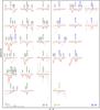 |
Fig. 7 Identified Zr iv (bottom of right panel), Zr v (left panel), and Zr vi (right panel) lines in the FUSE (λ < 1188 Å) and HST/STIS observations of RE 0503−289. The model (thick, red line) was calculated with an abundance of log Zr = −3.5. The dashed green spectrum was calculated without Zr. Prominent lines are marked, the Zr lines with their wavelengths from Tables A.9–A.11. |
The parameters adopted in our computations are summarized in Tables A.1–A.4 while computed and available experimental energies are compared in Tables A.5–A.8, for Zr iv–vii, respectively. Tables A.9–A.12 give the HFR weighted oscillator strengths (log gf) and transition probabilities (gA, in s-1) together with the numerical values (in cm-1) of the lower and upper energy levels and the corresponding wavelengths (in Å). In the last column of each table, we also give the cancellation factor, CF, as defined by Cowan (1981). We note that very low values of this factor (typically <0.05) indicate strong cancellation effects in the calculation of line strengths. In these cases, the corresponding gf and gA values could be very inaccurate and therefore need to be considered with some care. However, very few of the transitions appearing in Tables A.9–A.12 are affected. These tables are provided via the registered GAVO Tübingen Oscillator Strengths Service (TOSS7).
6.2. Zr line identification and abundance analysis
In the FUSE and HST/STIS observations of RE 0503−289, we identified Zr iv–vi lines (Table 4). The observation is well reproduced by our model calculated with a mass fraction of log Zr = −3.5 ± 0.2 (Fig. 7). The Zr iv/v/vi ionization equilibria are matched by our model.
Identified Zr lines in the UV spectrum of RE 0503−289.
In our synthetic spectra for G191−B2B, Zr IV λ 1598.948 Å is the strongest line. A comparison with the STIS spectrum shows that a Zr mass fraction of 2.6 × 10⁻⁶ (approximately 100 times solar, Grevesse et al. 2015) is the upper detection limit (Fig. 8).
7. Xenon
7.1. Oscillator-strength calculations for Xe IV, V, and VII ions
New calculations of oscillator strengths and radiative transition probabilities in xenon ions were also performed using the HFR+CPOL method (Cowan 1981; Quinet et al. 1999, 2002).
For Xe iv, the multiconfiguration expansion included 5s25p3, 5s25p26p, 5s25p2nf (n = 4–6), 5s25p5d6s, 5s25p5d6d, 5s25p6s2, 5s25p5d2, 5s25p4f2, 5s5p36s, 5s5p3nd (n = 5–6), 5s5p24f5d, and 5p5 for the odd parity, and 5s5p4, 5s25p2nd (n = 5–6), 5s25p26s, 5s25p2ng (n = 5–6), 5s25p5d6p, 5s25p5dnf (n = 4–6), 5s5p36p, 5s5p3nf (n = 4–6), and 5s5p25d2 for the even parity. The core-polarization effects were estimated with αd = 0.88 a.u. and rc = 0.86 a.u. which correspond to a Pd-like Xe ix ionic core. The former value was taken from Fraga et al. (1976) while the latter one corresponds to the HFR mean value ⟨ r ⟩ of the outermost core orbital (4d). The experimental energy levels published by Saloman (2004) were then used to optimize the radial parameters belonging to the 5p3, 5p26p, 5p24f, 5s5p4, 5p25d, and 5p26s configurations allowing us to reach average deviations between calculated and observed energies of 137 cm-1 and 251 cm-1, for odd and even parities, respectively.
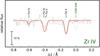 |
Fig. 8 Section of the STIS spectrum of G191−B2B around Zr ivλ 1598.948 Å compared with three synthetic spectra (thin, blue: no Zr, thick, red: Zr mass fraction = 2.6 × 10⁻⁶, dashed green: Zr = 2.6 × 10⁻⁵). |
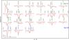 |
Fig. 9 Identified Xe vi (top three rows) and Xe vii (bottom row) lines in the FUSE (λ< 1188 Å) and HST/STIS observations of RE 0503−289. The model (thick, red line) was calculated with an abundance of log Xe = −3.9. The dashed, green spectrum was calculated without Xe. Prominent lines are marked (“is” denotes interstellar origin), and the Xe lines are labelled with their wavelengths given by Gallardo et al. (2015) and in Table B.7. |
In the case of Xe v, the following sets of configurations were considered in the HFR model: 5s25p2, 5s25p6p, 5s25pnf (n = 4–6), 5s25d6s, 5s25d6d, 5s26s2, 5s25d2, 5s24f2, 5s25f2, 5s5p26s, 5s5p2nd (n = 5–6), 5s5p6s6p, 5s5p6pnd (n = 5–6), 5s5p4fnd (n = 5–6), 5p4, 5p36p, and 5p3nf (n = 4–6) for the even parity, and 5s5p3, 5s25pnd (n = 5–6), 5s25pns (n = 6–7), 5s25png (n = 5–6), 5s25d6p, 5s25dnf (n = 4–6), 5s5p26p, 5s5p2nf (n = 4–6), 5s5p6snd (n = 5–6), 5s5p5d6d, 5s5p6s2, 5s5p5d2, 5p36s, and 5p3nd (n = 5–6) for the odd parity. The same core-polarization parameters as those used for Xe iv were used and the experimental energy levels reported by Saloman (2004) and Raineri et al. (2009) were incorporated into the semi-empirical fit to adjust the radial integrals corresponding to the 5p2, 5p6p, 5p4f, 5s5p3, 5p5d, 5p6d, 5p6s, and 5p7s configurations. In this process, we found mean deviations equal to 144 cm-1 in the even parity and 110 cm-1 in the odd parity.
For Xe vi, we used the same atomic data as those considered in one of our previous papers (Rauch et al. 2015a). More precisely, the radiative rates were taken from the work of Gallardo et al. (2015) who performed HFR+CPOL calculations including 35 odd-parity and 34 even-parity configurations, that is, 5s2np (n = 5–8), 5s2nf (n = 4–8), 5s2nh (n = 6–8), 5s28k, 5p2np (n = 6–8), 5p2nf (n = 4–8), 5p2nh (n = 6–8), 5p28k, 5s5p6s, 5s5pnd (n = 5–6), 5s5png (n = 5–6), 5p3, 5s5dnf (n = 4–5), 5s6snf (n = 4–5), and 5s5p2, 5s2ns (n = 6–8), 5s2nd (n = 5–8), 5s2ng (n = 5–8), 5s2ni (n = 7–8), 5p2nd (n = 5–8), 5p2ns (n = 6–8), 5p2ng (n = 5–8), 5p2ni (n = 7–8), 5s5pnf (n = 4–6), 5s4f2, 5s5f2, 5s5p6p, 4d95p4, respectively. In this latter study, the core-polarization effects were considered with two different ionic cores, that is, a Cd-like Xe vii core with αd = 5.80 a.u. for the 5s2nl–5s transitions, and a Pd-like Xe ix core with αd = 0.99 a.u. for all the other transitions. In their semi-empirical least-squares fitting process, Gallardo et al. (2015) achieved standard deviations with experimental energy levels of 149 cm-1 in the odd parity and 154 cm-1 in the even parity.
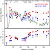 |
Fig. 10 Solar abundances (Asplund et al. 2009; Scott et al. 2015b,a; Grevesse et al. 2015, thick line; the dashed lines connect the elements with even and with odd atomic number) compared with the determined photospheric abundances of G191−B2B (blue circles, Rauch et al. 2013) and RE 0503−289 (red squares, Dreizler & Werner 1996; Rauch et al. 2012, 2014a,b, 2015a,b, 2016a,b, and this work). The uncertainties of the WD abundances are, in general, approximately 0.2 dex. The arrows indicate upper limits. Top panel: abundances given as logarithmic mass fractions. Bottom panel: abundance ratios to respective solar values, [X] denotes log (fraction/solar fraction) of species X. The dashed green line indicates solar abundances. |
Finally, for Xe vii, we used the same model as the one considered by Biémont et al. (2007) extending the set of oscillator strengths to weaker transitions (up to log gf>−8). As a reminder, these authors explicitly retained the following configurations in their configuration interaction expansions: 5s2, 5p2, 5d2, 4f2, 4fnp (n = 5–6), 4f6f, 4f6h, 5s6s, 5snd (n = 5–6), 5sng (n = 5–6), 5pnf (n = 5–6), 5p6p, 5p6h, 5d6s, 5d6d, and 5dng (n = 5–6) for the even parity, and 5snp (n = 5–6), 5snf (n = 4–6), 5s6h, 4f6s, 4fnd (n = 5–6), 4fng (n = 5–6), 5p6s, 5pnd (n = 5–6), 5png (n = 5–6), 5d6p, and 5dnf (n = 5–6), 5d6h for the odd parity. The same ionic core parameters as those used for Xe IV and Xe V ions were considered and all the experimental energy levels published by Saloman (2004) were included in the semi-empirical optimization of the radial parameters belonging to the 5s2, 5s6s, 5s5d, 5s6d, 5p2, 4f5p, 5s5p, 5s6p, 5s4f, 5s5f, 5p6s, and 5p5d configurations giving rise to standard deviations of 377 cm-1 and 250 cm-1 for even- and odd-parity levels, respectively.
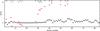 |
Fig. 11 Determined photospheric abundances of RE 0503−289 (cf. Fig. 10) compared with predictions for surface abundances of Karakas & Lugaro (2016, for an asymptotic giant branch (AGB) star with Minitial = 1.5 M⊙, Mfinal = 0.585 M⊙, metallicity Z = 0.014. [X/O] denotes the normalized log [(fraction of X/solar fraction of X)/(fraction of O/solar fraction of O)] mass ratio. The dashed green line indicates the solar ratio. |
The radial parameters used in our computations are summarized in Tables B.1, B.2 for the Xe iv–v ions, respectively. The calculated energy levels are compared with available experimental values in Tables B.3, B.4 while the HFR weighted oscillator strengths (log gf) and transition probabilities (gA in s-1) are reported in Tables B.5–B.7 for the Xe iv–v and vii ions, respectively. In the latter tables, we also give the numerical values (in cm-1) of lower and upper energy levels of each transition together with the corresponding wavelength (in Å) and the CF, as introduced in Sect. 6.1. These tables are provided via TOSS.
7.2. Xe line identification and abundance analysis
In the FUSE and HST/STIS observations of RE 0503−289, we identified Xe vi-vii lines (Table 5). The observation is well reproduced by our model, calculated with a mass fraction of log Xe = −3.9 ± 0.2 (Fig. 9). This is a factor of two higher than that previously determined by Werner et al. (2012b, log Xe = −4.2 ± 0.6 but agrees within their given error limits. The Xe vi/vii ionization equilibrium is matched by our model.
Identified Xe lines in the UV spectrum of RE 0503−289.
8. Results and conclusions
To search for Al lines in the observed UV spectrum of RE 0503−289, we created an extended Al model atom for our NLTE model-atmosphere calculations. We could only identify Al III λλ 1384.130 Å (Sect. 5), that was well suited to measure the Al abundance. It is reproduced at a solar value (−4.28 ± 0.2, mass fraction). This needs to be verified once better observations are available.
We identified Zr iv–vi lines in the observed high-resolution UV spectra RE 0503−289 (Table 4). These were well modeled using our newly calculated Zr iv–vii oscillator strengths. We determined a photospheric abundance of log Zr = −3.52 ± 0.2 (mass fraction, 1.5−4.8 × 10⁻⁴, 5775–14 480 times the solar abundance). This highly supersolar Zr abundance corresponds to the high abundances of other trans-iron elements in RE 0503−289 (Fig. 10). The Zr iv/v/vi ionization equilibria are well matched by our model (Teff = 70 000 K, log g = 7.5).
In addition to the previously discovered Xe vi–vii lines in the UV spectrum of RE 0503−289, we identified five new Xe vi lines. All identified Xe lines are well matched by our model with an abundance of log Xe = −3.88 ± 0.2 (mass fraction, 0.8−2.1 × 10⁻⁴, 4985–12 520 times the solar abundance). This highly supersolar Xe abundance is in line with abundances of other trans-iron elements in RE 0503−289 (Fig. 10).
The amount of trans-iron elements in the photosphere of RE 0503−289 strongly exceeds the yields of nucleosynthesis on the asymptotic giant branch (Fig 11). It is likely that radiative levitation is working efficiently in RE 0503−289 (Rauch et al. 2016a), increasing abundances by up to 4 dex compared with solar values.
The identification of lines of Zr and Xe and their precise abundance determinations only became possible after reliable transition probabilities for Zr iv–vii, Xe iv–v, and Xe vii were computed. Calculations for other, highly-ionized trans-iron elements are necessary to search for their lines and to measure their abundances.
The search for Zr and Xe lines in the UV spectrum of G191−B2B was entirely negative. We established an upper Zr abundance limit of approximately 100 times solar and confirmed the previously found upper limit for Xe of approximately 10 times solar (Rauch et al. 2016a).
Acknowledgments
T.R. and D.H. are supported by the German Aerospace Center (DLR, grants 05 OR 1507 and 50 OR 1501, respectively). The GAVO project had been supported by the Federal Ministry of Education and Research (BMBF) at Tübingen (05 AC 6 VTB, 05 AC 11 VTB) and is funded at Heidelberg (05 AC 11 VH3). Financial support from the Belgian FRS-FNRS is also acknowledged. P.Q. is research director of this organization. Some of the data presented in this paper were obtained from the Mikulski Archive for Space Telescopes (MAST). STScI is operated by the Association of Universities for Research in Astronomy, Inc., under NASA contract NAS5-26555. Support for MAST for non-HST data is provided by the NASA Office of Space Science via grant NNX09AF08G and by other grants and contracts. This research has made use of NASA’s Astrophysics Data System and the SIMBAD database, operated at CDS, Strasbourg, France. The TOSS service (http://dc.g-vo.org/TOSS) that provides weighted oscillator strengths and transition probabilities was constructed as part of the activities of the German Astrophysical Virtual Observatory.
References
- Asplund, M., Grevesse, N., Sauval, A. J., & Scott, P. 2009, ARA&A, 47, 481 [NASA ADS] [CrossRef] [Google Scholar]
- Biémont, É., Clar, M., Fivet, V., et al. 2007, Eur. Phys. J. D, 44, 23 [NASA ADS] [CrossRef] [EDP Sciences] [Google Scholar]
- Bohlin, R. C. 2007, in The Future of Photometric, Spectrophotometric and Polarimetric Standardization, ed. C. Sterken, ASP Conf. Ser., 364, 315 [Google Scholar]
- Cowan, R. D. 1981, in The theory of atomic structure and spectra (Berkeley, CA: University of California Press) [Google Scholar]
- Cowley, C. R. 1970, in The theory of stellar spectra (New York: Gordon & Breach) [Google Scholar]
- Cowley, C. R. 1971, The Observatory, 91, 139 [NASA ADS] [Google Scholar]
- Dreizler, S., & Werner, K. 1996, A&A, 314, 217 [NASA ADS] [Google Scholar]
- Fraga, S., Karwowski, J., & Saxena, K. M. S. 1976, in Handbook of Atomic Data (Amsterdam: Elsevier) [Google Scholar]
- Gallardo, M., Raineri, M., Reyna Almandos, J., Pagan, C. J. B., & Abrahão, R. A. 2015, ApJS, 216, 11 [NASA ADS] [CrossRef] [Google Scholar]
- Grevesse, N., Scott, P., Asplund, M., & Sauval, A. J. 2015, A&A, 573, A27 [NASA ADS] [CrossRef] [EDP Sciences] [Google Scholar]
- Holberg, J. B., Barstow, M. A., & Sion, E. M. 1998, ApJS, 119, 207 [NASA ADS] [CrossRef] [Google Scholar]
- Hubeny, I., Hummer, D. G., & Lanz, T. 1994, A&A, 282, 151 [NASA ADS] [Google Scholar]
- Hummer, D. G., & Mihalas, D. 1988, ApJ, 331, 794 [NASA ADS] [CrossRef] [Google Scholar]
- Karakas, A. I., & Lugaro, M. 2016, ApJ, 825, 26 [NASA ADS] [CrossRef] [Google Scholar]
- Khan, Z. A., Rahimullah, K., & Chaghtai, M. S. Z. 1981, Phys. Scr., 23, 843 [NASA ADS] [CrossRef] [Google Scholar]
- Khan, Z. A., Chaghtai, M. S. Z., & Rahimullah, K. 1983, J. Phys. B: At. Mol. Phys., 16, 1685 [NASA ADS] [CrossRef] [Google Scholar]
- Lemoine, M., Vidal-Madjar, A., Hébrard, G., et al. 2002, ApJS, 140, 67 [NASA ADS] [CrossRef] [Google Scholar]
- McCook, G. P., & Sion, E. M. 1999a, ApJS, 121, 1 [NASA ADS] [CrossRef] [Google Scholar]
- McCook, G. P., & Sion, E. M. 1999b, VizieR Online Data Catalog: III/210 [Google Scholar]
- Müller-Ringat, E. 2013, Dissertation, University of Tübingen, Germany, http://www.ivoa.net/documents/SimDM/index.html [Google Scholar]
- Quinet, P., Palmeri, P., Biémont, É., et al. 1999, MNRAS, 307, 934 [NASA ADS] [CrossRef] [EDP Sciences] [Google Scholar]
- Quinet, P., Palmeri, P., Biémont, É., et al. 2002, J. Alloys Comp., 344, 255 [CrossRef] [Google Scholar]
- Rahimullah, K., Chaghtai, M. S. Z., & Khatoon, S. 1978, Physica Scripta, 18, 96 [Google Scholar]
- Raineri, M., Gallardo, M., Padilla, S., & Reyna Almandos, J. 2009, J. Phys. B, 42, 205004 [NASA ADS] [CrossRef] [Google Scholar]
- Rauch, T., & Deetjen, J. L. 2003, in Stellar Atmosphere Modeling, eds. I. Hubeny, D. Mihalas, & K. Werner, ASP Conf. Ser., 288, 103 [Google Scholar]
- Rauch, T., Werner, K., Biémont, É., Quinet, P., & Kruk, J. W. 2012, A&A, 546, A55 [NASA ADS] [CrossRef] [EDP Sciences] [Google Scholar]
- Rauch, T., Werner, K., Bohlin, R., & Kruk, J. W. 2013, A&A, 560, A106 [NASA ADS] [CrossRef] [EDP Sciences] [Google Scholar]
- Rauch, T., Werner, K., Quinet, P., & Kruk, J. W. 2014a, A&A, 564, A41 [NASA ADS] [CrossRef] [EDP Sciences] [Google Scholar]
- Rauch, T., Werner, K., Quinet, P., & Kruk, J. W. 2014b, A&A, 566, A10 [NASA ADS] [CrossRef] [EDP Sciences] [Google Scholar]
- Rauch, T., Hoyer, D., Quinet, P., Gallardo, M., & Raineri, M. 2015a, A&A, 577, A88 [NASA ADS] [CrossRef] [EDP Sciences] [Google Scholar]
- Rauch, T., Werner, K., Quinet, P., & Kruk, J. W. 2015b, A&A, 577, A6 [NASA ADS] [CrossRef] [EDP Sciences] [Google Scholar]
- Rauch, T., Quinet, P., Hoyer, D., et al. 2016a, A&A, 587, A39 [NASA ADS] [CrossRef] [EDP Sciences] [Google Scholar]
- Rauch, T., Quinet, P., Hoyer, D., et al. 2016b, A&A, 590, A128 [NASA ADS] [CrossRef] [EDP Sciences] [Google Scholar]
- Reader, J., & Acquista, N. 1976, J. Opt. Soc. Am., 66, 896 [NASA ADS] [CrossRef] [Google Scholar]
- Reader, J., & Acquista, N. 1979, J. Opt. Soc. Am., 69, 239 [NASA ADS] [CrossRef] [Google Scholar]
- Reader, J., & Acquista, N. 1997, J. Opt. Soc. Am. B, 14, 1328 [NASA ADS] [CrossRef] [Google Scholar]
- Reader, J., & Lindsay, M. D. 2016, Phys. Scr., 91, 025401 [NASA ADS] [CrossRef] [Google Scholar]
- Saloman, E. B. 2004, J. Phys. Chem. Ref. Data, 33, 765 [NASA ADS] [CrossRef] [Google Scholar]
- Scott, P., Asplund, M., Grevesse, N., Bergemann, M., & Sauval, A. J. 2015a, A&A, 573, A26 [NASA ADS] [CrossRef] [EDP Sciences] [Google Scholar]
- Scott, P., Grevesse, N., Asplund, M., et al. 2015b, A&A, 573, A25 [NASA ADS] [CrossRef] [EDP Sciences] [Google Scholar]
- Werner, K., Deetjen, J. L., Dreizler, S., et al. 2003, in Stellar Atmosphere Modeling, eds. I. Hubeny, D. Mihalas, & K. Werner, ASP Conf. Ser., 288, 31 [Google Scholar]
- Werner, K., Dreizler, S., & Rauch, T. 2012a, Astrophysics Source Code Library [record ascl:1212.015] [Google Scholar]
- Werner, K., Rauch, T., Ringat, E., & Kruk, J. W. 2012b, ApJ, 753, L7 [NASA ADS] [CrossRef] [Google Scholar]
Appendix A: Additional tables for zirconium
Radial parameters (in cm-1) adopted for the calculations in Zr iv.
Radial parameters (in cm-1) adopted for the calculations in Zr v.
Radial parameters (in cm-1) adopted for the calculations in Zr vi.
Radial parameters (in cm-1) adopted for the calculations in Zr vii.
Comparison between available experimental and calculated energy levels in Zr iv.
Comparison between available experimental and calculated energy levels in Zr v.
Comparison between available experimental and calculated energy levels in Zr vi.
Comparison between available experimental and calculated energy levels in Zr vii.
Appendix B: Additional tables for xenon
Radial parameters (in cm-1) adopted for the calculations in Xe iv.
Radial parameters (in cm-1) adopted for the calculations in Xe v.
Comparison between available experimental and calculated energy levels in Xe iv.
Comparison between available experimental and calculated energy levels in Xe v.
All Tables
Column densities (in cm-2) and radial velocities (in km s-1) used to model interstellar clouds in the line of sight toward RE 0503−289.
Statistics of Zr iv–vii and Xe iv–v, vii atomic levels and line transitions from Tables A.9–A.12 and B.5–B.7, respectively.
Statistics of the Al model atom used in our calculations compared to our previous analyses (e.g., Rauch et al. 2013, 2016b).
Comparison between available experimental and calculated energy levels in Zr iv.
Comparison between available experimental and calculated energy levels in Zr v.
Comparison between available experimental and calculated energy levels in Zr vi.
Comparison between available experimental and calculated energy levels in Zr vii.
Comparison between available experimental and calculated energy levels in Xe iv.
Comparison between available experimental and calculated energy levels in Xe v.
All Figures
|
Fig. 1 Section of the STIS spectrum of RE 0503−289 with the interstellar Mg iiλλ 2796.35,2803.53 Å lines. |
| In the text | |
|
Fig. 2 Al ionization fractions in our G191−B2B model. m is the column mass, measured from the outer boundary of our model atmospheres. |
| In the text | |
|
Fig. 3 As Fig. 2, for RE 0503−289. |
| In the text | |
|
Fig. 4 Comparison of sections of the STIS spectra with our models for G191−B2B (top) and RE 0503−289 (bottom). The Al abundances are 1.1 × 10⁻⁵ (0.2 times the solar value, Rauch et al. 2013) and 5.3 × 10⁻⁵ (solar), respectively. In the top part, the green dashed line is a spectrum calculated without Al. Prominent lines are marked, the identified Al iii lines with their wavelengths. |
| In the text | |
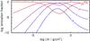 |
Fig. 5 Like Fig. 2, for Zr. |
| In the text | |
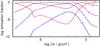 |
Fig. 6 Like Fig. 3, for Zr. |
| In the text | |
|
Fig. 7 Identified Zr iv (bottom of right panel), Zr v (left panel), and Zr vi (right panel) lines in the FUSE (λ < 1188 Å) and HST/STIS observations of RE 0503−289. The model (thick, red line) was calculated with an abundance of log Zr = −3.5. The dashed green spectrum was calculated without Zr. Prominent lines are marked, the Zr lines with their wavelengths from Tables A.9–A.11. |
| In the text | |
|
Fig. 8 Section of the STIS spectrum of G191−B2B around Zr ivλ 1598.948 Å compared with three synthetic spectra (thin, blue: no Zr, thick, red: Zr mass fraction = 2.6 × 10⁻⁶, dashed green: Zr = 2.6 × 10⁻⁵). |
| In the text | |
|
Fig. 9 Identified Xe vi (top three rows) and Xe vii (bottom row) lines in the FUSE (λ< 1188 Å) and HST/STIS observations of RE 0503−289. The model (thick, red line) was calculated with an abundance of log Xe = −3.9. The dashed, green spectrum was calculated without Xe. Prominent lines are marked (“is” denotes interstellar origin), and the Xe lines are labelled with their wavelengths given by Gallardo et al. (2015) and in Table B.7. |
| In the text | |
|
Fig. 10 Solar abundances (Asplund et al. 2009; Scott et al. 2015b,a; Grevesse et al. 2015, thick line; the dashed lines connect the elements with even and with odd atomic number) compared with the determined photospheric abundances of G191−B2B (blue circles, Rauch et al. 2013) and RE 0503−289 (red squares, Dreizler & Werner 1996; Rauch et al. 2012, 2014a,b, 2015a,b, 2016a,b, and this work). The uncertainties of the WD abundances are, in general, approximately 0.2 dex. The arrows indicate upper limits. Top panel: abundances given as logarithmic mass fractions. Bottom panel: abundance ratios to respective solar values, [X] denotes log (fraction/solar fraction) of species X. The dashed green line indicates solar abundances. |
| In the text | |
|
Fig. 11 Determined photospheric abundances of RE 0503−289 (cf. Fig. 10) compared with predictions for surface abundances of Karakas & Lugaro (2016, for an asymptotic giant branch (AGB) star with Minitial = 1.5 M⊙, Mfinal = 0.585 M⊙, metallicity Z = 0.014. [X/O] denotes the normalized log [(fraction of X/solar fraction of X)/(fraction of O/solar fraction of O)] mass ratio. The dashed green line indicates the solar ratio. |
| In the text | |
Current usage metrics show cumulative count of Article Views (full-text article views including HTML views, PDF and ePub downloads, according to the available data) and Abstracts Views on Vision4Press platform.
Data correspond to usage on the plateform after 2015. The current usage metrics is available 48-96 hours after online publication and is updated daily on week days.
Initial download of the metrics may take a while.