© ESO, 2017

1. Introduction

The combined BICEP2/Keck Array and Planck¹ analysis (BICEP2/Keck Array and Planck Collaborations 2015, hereafter BKP15), has confirmed that Galactic foregrounds likely constitute the dominant component of the B-mode polarization signal on a clean patch of the sky and at large scales (ℓ< 200). Characterization of these foregrounds is today the main limitation in the quest for the gravitational wave signature in the B-mode cosmic microwave background (CMB) power spectrum, i.e., for measuring the tensor-to-scalar ratio, r. This endeavour has been led by the analysis of the Galactic dust foregrounds carried out using Planck data (Planck Collaboration Int. XXX 2016, hereafter PIPXXX), and more recently of the synchrotron foregrounds using Planck and WMAP data (Planck Collaboration XXV 2016; Choi & Page 2015; Krachmalnicoff et al. 2016). It appears that Galactic thermal dust currently represents the major contaminant at high latitude in the spectral bands mainly adopted to search for the CMB signal by ground-based and balloon-borne experiments, i.e., between 100 and 220 GHz (Planck Collaboration Int. XXII 2015; Planck Collaboration X 2016).

The efficiency of Galactic dust cleaning for the cosmological B-mode analyses is based on two main factors: the accuracy of the Galactic polarized dust template; and the way it is extrapolated from the submillimetre to the millimetre bands. Recent forecasts of cosmological B-modes detection for ground-based, balloon-borne, and satellite experiments (Creminelli et al. 2015; Errard et al. 2016) appear to allow for very good sensitivity (down to r ≃ 2 × 10^-3) with only a few observational bands, when assuming a simple modelling of the foreground emission; however, other studies have shown that even in a global component separation framework, accurate modelling of the polarized dust spectral energy distribution (SED) is needed in order to reach the required very low levels of contamination of the cosmological B-modes by Galactic dust residuals (Armitage-Caplan et al. 2012; Remazeilles et al. 2016). Incorrect modelling of the dust SED would lead to biased estimates of the r parameter.

Several investigations to quantify the spatial variability of the polarized dust SED were initiated using the Planck data. A first estimate of the polarized dust spectral index was discussed in Planck Collaboration Int. XXII (2015) for regions at intermediate Galactic latitudes. Over 39% of the sky the averaged value was shown to be slightly higher than the dust spectral index in intensity, with a value of ${\mathit{\beta }}_{\mathrm{d}}^{\mathrm{P}}\mathrm{=}\mathrm{1.59}$, compared with ${\mathit{\beta }}_{\mathrm{d}}^{\mathrm{T}}\mathrm{=}\mathrm{1.51}$. More interestingly, an upper limit of its spatial dispersion was obtained by computing the standard deviation of the mean polarized dust spectral index estimated on 352 patches of 10° diameter, yielding a dispersion of 0.17. However, this estimate has been shown to be dominated by the expected Planck noise, and does not allow us to build a reliable model of these spatial variations.

A second early approach, in PIPXXX, investigated the correlation ratio between the 217 and 353 GHz Planck bands, which is a statistical measurement of the dust SED spatial variation, as we will discuss thoroughly in the following sections. This ratio was computed on large fractions of the sky and led to an upper limit of 7% decorrelation between 217 and 353 GHz. An initial estimate of the impact of a possible dust polarization decorrelation between frequencies, due to a spatial variation of its SED, was performed in the BKP15 analysis. A loss of 10% in the 150 GHz × 353 GHz cross-spectrum in the joint analysis, due to the decorrelation, was estimated to produce a positive bias of 0.018 on the determination of r.

In this new study, we present an improved analysis of the correlation ratio between the 353 GHz and 217 GHz Planck bands as a tracer of the spatial variations of the polarized dust SED. We derive new constraints on these variations and look at the impact they would have on the determination of the cosmological B-mode signal.

This paper is organized as follows. We present the data used in this work in Sect. 2. The analysis of the dust polarization correlation ratio is described in Sect. 3. The impact of the polarized dust decorrelation on the determination of the tensor-to-scalar ratio r is illustrated in Sect. 4. We discuss the possible origin of the spatial variations of the polarized dust SED in Sect. 5, before concluding in Sect. 6.

2. Data and region selection

2.1. Planck data

In this paper, we use the publicly available Planck High Frequency Instrument (HFI) data at 217 GHz and 353 GHz (Planck Collaboration I 2016). The signal-to-noise ratio of dust polarization in the Planck-HFI maps at lower frequencies does not allow us to derive significant results in the framework adopted for this study and consequently the other channels are not used. These data consist of a set of maps of the Stokes Q and U parameters at each frequency, projected onto the HEALPix pixelization scheme (Górski et al. 2005). The maps and their properties are described in detail in Planck Collaboration VIII (2016).

We also use subsets of these data in order to exploit the statistical independence of the noise between them. As described in Planck Collaboration VIII (2016), the data were split into either the time or the detector domains. In this paper we use two particular data splits.

• The “detector-set” maps (hereafter DS, also sometimes called “DetSets”). Planck-HFI measures the sky polarization thanks to polarization sensitive bolometers (PSBs), which are each sensitive to one direction of polarization. PSBs are assembled in pairs, the angle between two PSBs in a pair being 90° and the angle between two pairs being 45°, allowing for the reconstruction of Stokes I, Q, and U. Four such pairs are available at 217 and 353 GHz. These were split into two subsets of two pairs (four bolometers) to produce two noise-independent sets of Q and U maps called “detector-sets”, for each frequency band.

• The “half-mission” maps (hereafter HM). Planck-HFI completed five independent full-sky surveys over 30 months. Surveys 1 and 2 constitute the Planck “nominal mission” and this was repeated a second time during Surveys 3 and 4. A fifth survey was performed with a different scanning strategy, but was not included in the released half-mission maps. Thus, Planck-HFI data can be split into two noise-independent sets of Q and U maps, labelled “HM1” and “HM2”, for each frequency band.

2.2. Region selection

In order to focus on the most diffuse areas of the Galactic dust emission, we have performed our analysis on various fractions of the sky using the set of science regions introduced in PIPXXX. These regions have been constructed to reject regions with CO line brightness I_CO ≥ 0.4 K km s^-1. The complement to this mask by itself defines a preliminary region that retains a sky fraction f_sky = 0.8. In combination with thresholding, based on the Planck 857 GHz intensity map, six further preliminary regions are defined over f_sky = 0.2 to 0.7 in steps of 0.1. After point source masking and apodization, this procedure leads to the large retained (LR) regions LR16, LR24, LR33, LR42, LR53, LR63, and LR72, where the numbers denote the net effective sky coverages as a percentage, i.e., $\mathrm{100}\hspace{0.17em}{\mathit{f}}_{\mathrm{sky}}^{\mathrm{eff}}\mathit{.}$ We note that the highest-latitude and smallest region, LR16, is an addition to those defined in PIPXXX, following the same procedure. Furthermore, LR63 has been split into its north and south Galactic hemisphere portions, yielding LR63N and LR63S, covering ${\mathit{f}}_{\mathrm{sky}}^{\mathrm{eff}}\mathrm{=}\mathrm{0.33}$ and 0.30, respectively. All of these regions are shown in Fig. 1.

As previously stated in PIPXXX, the dust polarization angular power spectra computed on these regions can be considered to be approximately statistically independent because most of the power arises from the brightest 10% of a given region, the same 10% that differentiates one (preliminary) region from another.

More specifically, for the ${\mathit{C}}_{\mathit{\ell }}^{\mathit{BB}}$ power spectra computed with the 353 GHz Planck data, the difference (non-overlapping) region LRx_i−LRx_i−1, i> 1 (about 10% of the sky, by definition), contains more than 75% of the power computed on LRx_i, for x ∈ { 24,33,42,53,63,72 }. LR63N and LR63S are independent of one another, but not of LR63. Nevertheless, we prefer to utilize the overlapping regions (which are not fully statistically independent) in order to be able to relate the present work to the previous Planck analyses in general and to PIPXXX in particular. These masks are publicly available through the Planck Legacy Archive².

2.3. Simulations

The simulated polarization maps presented in this work were built using a simplified two-component model consisting of dust plus CMB, both simulated as stochastic realizations with a Gaussian distribution. CMB maps are defined as realizations based on the Planck Collaboration best-fit ΛCDM model (Planck Collaboration XIII 2016), assuming a tensor-to-scalar ratio r = 0 and an optical depth τ = 0.06 (Planck Collaboration Int. XLVII 2016; Planck Collaboration Int. XLVI 2016). The dust component maps at 353 GHz are defined as Gaussian realizations using a power-law model of the EE and BB angular power spectra (with a spectral index equal to −0.42 and amplitudes matching those in Table 1 of PIPXXX), following the prescriptions of PIPXXX, and normalized for each region of the sky introduced in Sect. 2.2. Dust maps at other frequencies are scaled with a constant modified blackbody spectrum with ${\mathit{\beta }}_{\mathrm{d}}^{\mathrm{P}}\mathrm{=}\mathrm{1.59}$ and T_d = 19.6 K (Planck Collaboration Int. XVII 2014; Planck Collaboration Int. XXII 2015). The results of this paper have also been confronted with realistic dust simulations (non-Gaussian, described in Vansyngel et al. 2016) finding statistical significances and probabilities-to-exceed (PTEs) similar to the ones obtained with the Gaussian realizations of the dust.

Fig. 1 Masks and complementary science regions that retain fractional coverage of the sky, fsky, from 0.8 to 0.2 (see details in Sect. 2.2). The grey is the CO mask, whose complement is a selected region with fsky = 0.8. In increments of fsky = 0.1, the retained regions can be identified by the colours from yellow (0.3) to blue (0.8). The LR63N and LR63S regions are displayed in black and white, respectively, and the LR63 region is the union of the two. Also shown is the (unapodized) point source mask used.

The instrumental noise component is then introduced in each pixel using the Planck Q and U covariance maps at 217 and 353 GHz, associated with the DS and HM data set-ups. Using a set of 1000 simulations, we checked that the instrumental noise in the range of multipoles ℓ = 50–700 built from covariances was consistent with the Full Focal Plane Monte Carlo noise simulations, namely FFP8 (Planck Collaboration XII 2016) at 217 and 353 GHz, which are publicly available through the Planck Legacy Archive². For each of the regions described in Sect. 2.2, we built 1000 independent dust, CMB and noise realizations with these properties.

We note that we did not directly use the FFP8 maps in this analysis because of two issues with the polarized dust component in the Planck Sky Model (PSM, Delabrouille et al. 2013) used to build these simulations. First, the polarized dust maps include Planck instrumental noise because they are computed from the Planck 353 GHz maps smoothed to 30′. This contribution significantly enhances the apparent dust signal at high Galactic latitudes, where the signal-to-noise ratio of the data is low at this resolution. Second, the polarized dust component in the PSM already includes spatial variations of the polarized dust spectral index. Thus, it cannot be used to perform a null-test for no spatial variation of the SED.

3. The dust polarization correlation ratio

3.1. Definition

We statistically estimate the spatial variation of the dust SED by constructing the correlation ratio for the dust between 217 and 353 GHz, as a function of the multipole ℓ. This is defined as the ratio of the cross-spectrum between these bands and the geometric mean of the two auto-spectra in the same bands, i.e., 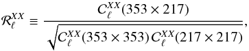${\mathrm{ℛ}}_{\mathit{\ell }}^{\mathit{XX}}\mathrm{\equiv }\frac{{\mathrm{𝒞}}_{\mathit{\ell }}^{\mathit{XX}}\mathrm{(}\mathrm{353}\mathrm{\times }\mathrm{217}\mathrm{)}}{\sqrt{{\mathrm{𝒞}}_{\mathit{\ell }}^{\mathit{XX}}\mathrm{(}\mathrm{353}\mathrm{\times }\mathrm{353}\mathrm{)}\hspace{0.17em}{\mathrm{𝒞}}_{\mathit{\ell }}^{\mathit{XX}}\mathrm{(}\mathrm{217}\mathrm{\times }\mathrm{217}\mathrm{)}}}\mathit{,}$(1)where X ∈ { E,B }. If the maps at 217 and 353 GHz contain only dust and the dust SED is constant over the region for which the power spectra are computed, then ${\mathrm{ℛ}}_{\mathit{\ell }}^{\mathit{XX}}\mathrm{=}\mathrm{1}$. However, if the dust is not the only component to contribute to the sky polarization or if the dust SED varies spatially, then the ratio is expected to deviate from unity. Nevertheless, the spatial variations of the SED, as we see in the next subsection, do not affect the ratio ${\mathrm{ℛ}}_{\mathit{\ell }}^{\mathit{XX}}$ at the largest scales. This is the reason why the study in PIPXXX (where the ratio ${\mathrm{ℛ}}_{\mathit{\ell }}^{\mathit{XX}}$ was computed from the fitted amplitude of power laws dominated by the largest scales) found no significant deviation from unity. In what follows we conduct this analysis for ℓ> 50 to avoid any significant contribution from Planck systematics effects at low ℓ (Planck Collaboration VIII 2016).

In order to avoid any bias issues due to the noise auto-correlation, and in order to minimize the systematic effects, the auto- and cross-spectra are computed using independent sets of Planck data, namely the half-mission and detector-set maps (Planck Collaboration VIII 2016). Hence the auto-spectra are computed for frequency ν as 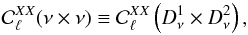${\mathrm{𝒞}}_{\mathit{\ell }}^{\mathit{XX}}\mathrm{(}\mathit{\nu }\mathrm{\times }\mathit{\nu }\mathrm{)}\mathrm{\equiv }{\mathrm{𝒞}}_{\mathit{\ell }}^{\mathit{XX}}\mathrm{(}{\mathit{D}}_{\mathit{\nu }}^{\mathrm{1}}\mathrm{\times }{{\mathit{D}}_{\mathit{\nu }}^{\mathrm{2}}}^{\mathrm{)}}\mathit{,}$(2)where ${\mathit{D}}_{\mathit{\nu }}^{\mathrm{1}}$ and ${\mathit{D}}_{\mathit{\nu }}^{\mathrm{2}}$ are the two independent sets of data, e.g., DS1 and DS2, or HM1 and HM2 (see Sect. 2.1). Similarly, the cross-spectra between two frequencies, ν₁ and ν₂, are given by 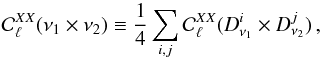${\mathrm{𝒞}}_{\mathit{\ell }}^{\mathit{XX}}\mathrm{(}{\mathit{\nu }}_{\mathrm{1}}\mathrm{\times }{\mathit{\nu }}_{\mathrm{2}}\mathrm{)}\mathrm{\equiv }\frac{\mathrm{1}}{\mathrm{4}}\sum _{\mathit{i,j}}{\mathrm{𝒞}}_{\mathit{\ell }}^{\mathit{XX}}\mathrm{(}{\mathit{D}}_{{\mathit{\nu }}_{\mathrm{1}}}^{\mathit{i}}\mathrm{\times }{\mathit{D}}_{{\mathit{\nu }}_{\mathrm{2}}}^{\mathit{j}}\mathrm{)}\hspace{0.17em}\mathit{,}$(3)where the indices i and j take the values 1 and 2. The results are labelled “HM” or “DS” when obtained using the half-mission or detector-set maps, respectively.

The spectra have been computed using Xpol (Tristram et al. 2005), which is a polarization pseudo-C_ℓ estimator that corrects for incomplete sky coverage and pixel and beam window functions.

3.2. Planck measurements

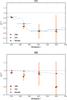Fig. 2 Dust polarization correlation ratios ${\mathrm{ℛ}}_{\mathit{\ell }}^{\mathit{EE}}$ (top panel) and ${\mathrm{ℛ}}_{\mathit{\ell }}^{\mathit{BB}}$ (bottom panel) between 217 and 353 GHz, computed on the LR63 region. The correlation ratios determined from the detector-set data (DS) splits are shown as yellow squares and the ratios computed from the half-mission (HM) splits as red diamonds. The correlation ratio expectations for the model described in Eq. (5) are shown as blue dashed lines (blue circles when binned as the data). Horizontal blue segments in the top panel represent the range of the ℓ bins. The uncertainties have been estimated as the median absolute deviation over a set of 1000 simulations (see Sect. 2.3) of CMB, dust, and Gaussian noise.

The EE and BB dust correlation ratios obtained in four multipoles ranges (ℓ = [50,160], [160,320], [320,500], and [500,700]) are shown in Fig. 2 for the Planck HM and DS data versions, and a fraction of the sky f_sky = 0.7, i.e., the LR63 region.

Since the definition of the correlation ratio, ${\mathrm{ℛ}}_{\mathit{\ell }}^{\mathit{XX}}$, uses non-linear operations (such as ratio and square root), the associated uncertainties are not trivial to estimate and so are determined from the median absolute deviation of 1000 Monte Carlo noise realizations, including Planck instrumental noise, as detailed in Sect. 2.3.

The correlation ratios between the 217 and 353 GHz bands that might be expected are computed using the simulation set-up introduced in Sect. 2.3, and defined by a two-component modelling of dust plus CMB signals, assuming no spatial variations of the dust SED and no noise. If we suppose that the Planck maps at 217 and 353 GHz are a sum of CMB and dust components, then (in thermodynamic units and assuming no instrumental noise) we have

$\begin{array}{ccc}& & {\mathit{M}}_{\mathrm{353}}\mathrm{=}{\mathit{M}}_{\mathrm{dust}}\mathrm{+}{\mathit{M}}_{\mathrm{CMB}}\mathit{,}\\ & & {\mathit{M}}_{\mathrm{217}}\mathrm{=}\mathit{\alpha }{\mathit{M}}_{\mathrm{dust}}\mathrm{+}{\mathit{M}}_{\mathrm{CMB}}\mathit{,}\end{array}$(4)

where M_dust is the dust map at 353 GHz, M_CMB is the CMB map, α is a constant scaling coefficient representing the dust SED, and M can represent the Stokes parameters Q and U. Then, combining Eqs. (1) and (4) and assuming that the dust and CMB components are not spatially correlated, the expected correlation ratio becomes $\mathrm{ℛ̂}\begin{array}{c}\mathit{XX}\\ \mathit{\ell }\end{array}\mathrm{=}\frac{\mathit{\alpha }\hspace{0.17em}{\mathrm{𝒞}}_{\mathit{\ell ,}\mathrm{dust}}^{\mathit{XX}}\mathrm{+}{\mathrm{𝒞}}_{\mathit{\ell ,}\mathrm{CMB}}^{\mathit{XX}}}{{\left[{\mathit{\alpha }}^{\mathrm{2}}{\mathrm{(}{{\mathrm{𝒞}}_{\mathit{\ell ,}\mathrm{dust}}^{\mathit{XX}}}^{\mathrm{)}}}^{\mathrm{2}}\mathrm{+}{\mathrm{(}{{\mathrm{𝒞}}_{\mathit{\ell ,}\mathrm{CMB}}^{\mathit{XX}}}^{\mathrm{)}}}^{\mathrm{2}}\mathrm{+}\mathrm{(}\mathrm{1}\mathrm{+}{\mathit{\alpha }}^{\mathrm{2}}\mathrm{)}\hspace{0.17em}{\mathrm{𝒞}}_{\mathit{\ell ,}\mathrm{dust}}^{\mathit{XX}}{\mathrm{𝒞}}_{\mathit{\ell ,}\mathrm{CMB}}^{\mathit{XX}}\right]}^{\mathrm{1}\mathit{/}\mathrm{2}}}\mathit{,}$(5)where X ∈ { E,B }. It can clearly be seen that even if α is a constant, the CMB component will make the correlation ratio ℛ ≠ 1. The model power spectra corresponding to Eq. (5) are also shown in Fig. 2.

The PlanckEE data match the expected EE correlation ratio and are strongly dominated by the CMB signal. Two approaches have been considered for removing the CMB component from the correlation ratio in order to see the effect of the dust decorrelation in the EE spectra, namely analysis in pixel space or in multipole space. The noise on the CMB template, subtracted from the Planck maps, would produce an auto-correlation of the noise when building the correlation ratios and would strongly impact our analysis in polarization; this argues against using the first (pixel-based) option. Moreover, the second option, which consists of correcting the 217 and 353 GHz Planck cross-spectra by subtracting a model of the CMB power spectrum, is affected by the cosmic variance of the CMB, which is dominant compared to the dust component in the EE correlation ratios. For all these reasons, in the following analysis we focus on the multipole-based BB modes only, where the CMB component (coming from the lensing B-modes, Planck Collaboration Int. XLI 2016) is subdominant compared to the observed signal.

As can be seen in the lower panel of Fig. 2, the BB correlation ratios, ${\mathrm{ℛ}}_{\mathit{\ell }}^{\mathit{BB}}$, exhibit a clear deficit compared to the expected model; this is discussed in more detail in the next section. We have also carried out similar analyses of the other regions defined in Sect. 2.2. The same deficit can be seen in Fig. 3, where the results averaged over the lowest multipole bin are shown as a function of the mean column density (see Table 1).

3.3. Significance of the Planck measurements

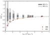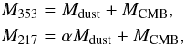
Fig. 3 Dependence of the Planck correlation ratios with the mean column density of the region on which they are computed in the first multipole bin (ℓ = [50,160]). The HM and DS measurements can be compared to the theoretical expectations (including dust and CMB, as in Eq. (5)) shown as blue segments. The grey bars give the 68% and 95% confidence levels computed over 1000 realizations of dust, CMB, and Gaussian noise. The column density dependence fit by a power law (see Eq. (6)) is shown as a dashed line.

The significance of the Planck data correlation ratios can be quantified using the distribution of ${\mathrm{ℛ}}_{\mathit{\ell }}^{\mathit{BB}}$ computed with simulations including Planck instrumental noise at 217 and 353 GHz. Since the denominator of ${\mathrm{ℛ}}_{\mathit{\ell }}^{\mathit{BB}}$ can get close to zero, the distribution of the correlation ratios from dust, CMB, and noise can be highly non-Gaussian. For this reason, we cannot give symmetrical error bars and significance levels expressed in terms of σ. Instead we use the PTE, which makes no assumption about the shape of the distribution. As we will see, the Planck measurements of the correlation ratios in the DS and HM data sets appear systematically smaller than the most probable correlation ratio in our simulations that include instrumental noise.

The impact of the CMB and the noise on the correlation ratio can be seen in Fig. 3 via the grey vertical histograms. These data are based on the correlation ratios obtained on a set of 1000 Monte Carlo realizations, including Gaussian Planck noise on top of the simulated CMB and dust components (see Sect. 2.3). The distributions of the simulated correlation ratios are available for all multipole ranges and regions in Appendix A (in Figs. A.1–A.9). While noise barely affects the most probable ratios in the first multipole bin (ℓ = 50–160) when compared to the theoretical expectation (blue), it can create an important level of decorrelation in the other bins, particularly in the smallest regions (up to an additional 30% in the fourth multipole bin for LR16).

In order to quantify the significance of the Planck measurements with respect to the simulated decorrelation from CMB and noise, we compute the PTE, defined as the probability of a simulation having more decorrelation (i.e., smaller correlation ratio) than the data. This is computed as the fraction of the 1000 realizations having a correlation ratio smaller than the Planck measurements, for each multipole bin and HM/DS case. These PTEs are listed in Table 1. We also compute a combined PTE over all multipole bins, defined as the probability of obtaining correlation ratios smaller than Planck measurements simultaneously in all four multipole bins (50 < ℓ < 700).

The combined PTEs (for 50 < ℓ < 700) are < 1.5% for the DS case and <0.1% for the HM case. When focusing on individual multipole bins, the detection level is not as strong; the PTE values range between 0.6% and 11.2% in the first multipole bin (50 < ℓ < 160) for both DS and HM cases. In the second multipole bin (160 < ℓ < 320), the DS correlation ratio PTEs range from 11.5 to 47.4%, while for the HM case they range from 1.1 to 39.9% (with significant PTEs on several regions though). The third and fourth multipole bins (320 <ℓ < 700) show no significant evidence of decorrelation.

The significant excess of decorrelation in the Planck data between 217 and 353 GHz, especially in the first multipole bin (50 < ℓ < 160) is consequently very unlikely to be attributable to CMB or to instrumental noise (or to systematic effects, see next section). We therefore conclude that this excess is a statistical measurement of the spatial variation of the polarized dust SED.

3.4. Impact of systematic effects

Since we have restricted our analysis to multipoles ℓ > 50, the 217 and 353 GHz cross-spectra are not significantly affected by those systematic effects that are most important at low multipoles, such as the ADC non-linearity correction or the dipole and calibration uncertainties (Planck Collaboration VII 2016; Planck Collaboration VIII 2016). However, the Planck cross-spectra in the multipole range 50 < ℓ < 700 could be affected by beam systematics. Thanks to its definition, the correlation ratio should be approximately independent of the beam uncertainty, because of the presence of the same beam functions, ${\mathrm{ℬ}}_{\mathit{\ell }}^{\mathrm{353}}$ and ${\mathrm{ℬ}}_{\mathit{\ell }}^{\mathrm{217}}$, in the numerator and denominator. A further systematic contribution could arise from the difference between the beam function of the 353 × 217 cross-spectra, ${\mathrm{ℬ}}_{\mathit{\ell }}^{\mathrm{353}\mathrm{\times }\mathrm{217}}$, and the product of the independent beam functions, ${\mathrm{ℬ}}_{\mathit{\ell }}^{\mathrm{353}}\mathrm{\times }{\mathrm{ℬ}}_{\mathit{\ell }}^{\mathrm{217}}$. We have checked that this ratio exhibits a very low departure from unity, at the 10^-5 level, which cannot reproduce the amplitude of the observed Planck correlation ratio. We also checked that the correction of the bandpass mismatch in the 217 and 353 GHz bands does not affect the correlation ratio. The same analysis has been reproduced using two versions of the bandpass mismatch corrections (see Planck Collaboration VII 2016), yielding results consistent down to 0.1%.

We use the two splits, HM and DS, as indicators of the level of residuals due to systematic effects in our analysis. This can be assessed by examining Figs. A.1 to A.9. While the HM and DS correlation ratios are very consistent in the first and last multipole bins (ℓ = 50–160, and ℓ = 500–700), they are not as consistent for the second multipole bin, (ℓ = 160–320). This apparent discrepancy is not explained by the current knowledge of any systematic effects in Planck, and so indicates the need for some caution.

3.5. Dependence on column density

For CMB polarization studies, it is important to characterize the dependence of the observed decorrelation ratio on column density. The Planck correlation ratios in the first multipole bin (ℓ = [50,160]), obtained on the various science regions, are shown in Fig. 3 as a function of the mean column density, N_{H i}, computed for each region as the average over the unmasked pixels of the Planck column density map, assuming a constant opacity τ/N_{H i} (Planck Collaboration XI 2014). The HM and DS measurements of the PlanckBB correlation ratio can be compared to the theoretical expectation (blue segment) and the dispersion due to noise (grey histograms) computed over 1000 Monte Carlo realizations including Gaussian noise (see Sect. 2.3). We recall (see Sect. 2.2) that measurements of the correlation ratio obtained in different regions can be considered statistically independent to a good approximation (except for LR63 with respect to LR63N or LR63S).

In this first multipole bin (50 < ℓ < 160), where the primordial B-mode signal is expected, the BB correlation ratio of the DS and HM cases can be described well by a power law of N_{H i}: ${\mathrm{ℛ}}_{\mathrm{50}\mathrm{-}\mathrm{160}}^{\mathit{BB}}\mathrm{=}\mathrm{1}\mathrm{-}{\mathit{K}}_{\mathrm{50}\mathrm{-}\mathrm{160}}^{\mathit{BB}}{\left(\frac{{\mathit{N}}_{\mathrm{H}\hspace{0.17em}{i}}}{{\mathrm{10}}^{\mathrm{20}}}\right)}^{\mathit{\gamma }}\mathit{,}$(6)with ${\mathit{K}}_{\mathrm{50}\mathrm{-}\mathrm{160}}^{\mathit{BB}}\mathrm{=}\mathrm{0.40}\mathrm{\pm }\mathrm{0.32}$ and γ = −1.76 ± 0.69. Hence the more diffuse the Galactic foregrounds, the stronger the decorrelation between 217 and 353 GHz. This is an important issue for CMB analyses, which mainly focus on the most diffuse regions of the sky in order to minimize the contamination by Galactic dust emission.

4. Impact on the CMB B-modes

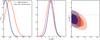Fig. 4 ${\mathit{C}}_{\mathit{\ell }}^{\mathit{BB}}$ spectra likelihood posteriors on the r and Ad parameters derived from the simulations of the BICEP2-Keck and Planck 353 GHz data, using: 150 and 353 GHz channels (BKP, red); and 95, 150 and 353 GHz channels (BK(+95), blue). The 1D posteriors of r (marginalized over ${\mathit{\beta }}_{\mathrm{d}}^{\mathrm{P}}$ and Ad) and of Ad (marginalized over ${\mathit{\beta }}_{\mathrm{d}}^{\mathrm{P}}$ and r) are shown in the left and middle panels (blue and red lines, respectively). The input value in our simulations for the dust amplitude at 353 GHz (4.5 μK2 at ℓ = 80) is indicated as a dashed line. The 2D posterior marginalized over ${\mathit{\beta }}_{\mathrm{d}}^{\mathrm{P}}$ is presented in the right panel (68% in darker shading and 95% in lighter shading).

In Sect. 3 we show that the correlation of the dust polarization B-modes between 217 and 353 GHz can depart significantly from unity for multipoles ℓ ≳ 50. This decorrelation, as previously noted by, e.g., Tassis & Pavlidou (2015) or BKP15, will have an impact on the search for CMB primordial B-modes that assume a constant dust polarization SED over the region of sky considered. In order to quantify this effect, we use toy model simulations of the BICEP2/Keck and Planck data, introducing a decorrelation between the 150 and the 353 GHz channels that matches our results in Sect. 3. This analysis is intended to be illustrative only, and not to be an exact reproduction of the work presented in BICEP2/Keck Array and Planck Collaborations (2015) and BICEP2 and Keck Array Collaborations (2016).

We approximate the likelihood analyses presented in BKP15 and BICEP2 and Keck Array Collaborations (2016) using simple simulations of the CMB and dust ${\mathit{C}}_{\mathit{\ell }}^{\mathit{BB}}$ angular power spectra. We directly simulate the 150 × 150, 150 × 353, and 353 × 353${\mathit{C}}_{\mathit{\ell }}^{\mathit{BB}}$ angular power spectra (where the Planck 353 GHz spectrum comes from two noise-independent detector-set subsamples). In order to include the noise contribution from these experiments and to perform a Monte Carlo analysis over 2000 simulations, we add the sample variance and the noise contribution to the spectra as a Gaussian realization of 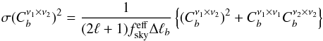$\mathit{\sigma }\mathrm{(}{\mathit{C}}_{\mathit{b}}^{{\mathit{\nu }}_{\mathrm{1}}\mathrm{\times }{\mathit{\nu }}_{\mathrm{2}}}{\mathrm{)}}^{\mathrm{2}}\mathrm{=}\frac{\mathrm{1}}{\mathrm{(}\mathrm{2}\mathit{\ell }\mathrm{+}\mathrm{1}\mathrm{)}{\mathit{f}}_{\mathrm{sky}}^{\mathrm{eff}}\mathrm{\Delta }{\mathit{\ell }}_{\mathit{b}}}\mathrm{\left\{}\mathrm{\right(}{\mathit{C}}_{\mathit{b}}^{{\mathit{\nu }}_{\mathrm{1}}\mathrm{\times }{\mathit{\nu }}_{\mathrm{2}}}{\mathrm{)}}^{\mathrm{2}}\mathrm{+}{\mathit{C}}_{\mathit{b}}^{{\mathit{\nu }}_{\mathrm{1}}\mathrm{\times }{\mathit{\nu }}_{\mathrm{1}}}{{\mathit{C}}_{\mathit{b}}^{{\mathit{\nu }}_{\mathrm{2}}\mathrm{\times }{\mathit{\nu }}_{\mathrm{2}}}}^{\mathrm{\}}}$(7)for each power spectra C_b computed in an ℓ-centred bin of size Δℓ_b, where ${\mathit{f}}_{\mathrm{sky}}^{\mathrm{eff}}$ is the effective sky fraction, ${\mathit{C}}_{\mathit{b}}^{{\mathit{\nu }}_{\mathrm{1}}\mathrm{\times }{\mathit{\nu }}_{\mathrm{1}}}$ and ${\mathit{C}}_{\mathit{b}}^{{\mathit{\nu }}_{\mathrm{2}}\mathrm{\times }{\mathit{\nu }}_{\mathrm{2}}}$ are the signal plus noise auto-power spectra in the frequency bands ν₁ and ν₂, respectively, and ${\mathit{C}}_{\mathit{b}}^{{\mathit{\nu }}_{\mathrm{1}}\mathrm{\times }{\mathit{\nu }}_{\mathrm{2}}}$ is the signal-only cross-power spectrum between these two frequencies (supposing the noise to be uncorrelated between the two bands); although the noise affects the variance of the C_ℓ, we note that it does not affect its mean value, since we cross-correlate noise-independent maps.

The CMB ${\mathit{C}}_{\mathit{\ell }}^{\mathit{BB}}$ spectrum is generated from a Planck 2015 best-fit ΛCDM model (Planck Collaboration XIII 2016) with no tensor modes (r = 0). The dust for the 353 × 353 power spectrum is constructed as a power law in ℓ, specifically ℓ^-0.42 following PIPXXX. The amplitude of this spectrum at ℓ = 80 is taken to be A_d = 4.5 μK². This is an ad hoc value chosen to lie between the predicted PIPXXX value in the BICEP2 region (A_d = 13.4 ± 0.26 μK²), and the BKP15 value (${\mathit{A}}_{\mathrm{d}}\mathrm{=}\mathrm{3.}{\mathrm{3}}_{-0.8}^{\mathrm{+}\mathrm{0.9}}\hspace{0.17em}\mathit{\mu }{\mathrm{K}}^{\mathrm{2}}$, marginally compatible with our chosen value, which could be underestimated if some decorrelation exists). A single modified blackbody spectrum is applied to scale the dust 353 GHz ${\mathit{C}}_{\mathit{\ell }}^{\mathit{BB}}$ spectrum to the other frequencies, with ${\mathit{\beta }}_{\mathrm{d}}^{\mathrm{P}}\mathrm{=}\mathrm{1.59}$ and T_d = 19.6 K.

Finally, we introduce a decorrelation factor ${\mathrm{ℛ}}_{\mathit{\ell }}^{\mathit{BB}}$ in our simulated cross-spectra, which we chose to be constant in ℓ. If we make the assumption that the SED spatial variations come from spatial variations of the dust spectral index around its mean value (see Sect. 5.1), a first-order expansion gives a frequency dependence of (1−ℛ^BB) that scales as [ln(ν₁/ν₂)] ². We explored many values for the ${\mathrm{ℛ}}_{\mathit{\ell }}^{\mathit{BB}}$ ratio and we have chosen to present here the results we obtain for a correlation ratio between 150 and 353 GHz of ${\mathrm{ℛ}}_{\mathit{\ell }}^{\mathit{BB}}\mathrm{\left(}\mathrm{150}\mathit{,}\mathrm{353}\mathrm{\right)}\mathrm{=}\mathrm{0.85}$. With the frequency scaling of [ln(ν₁/ν₂)] ², this ratio becomes ${\mathrm{ℛ}}_{\mathit{\ell }}^{\mathit{BB}}\mathrm{\left(}\mathrm{217}\mathit{,}\mathrm{353}\mathrm{\right)}\mathrm{=}\mathrm{0.95}$, ${\mathrm{ℛ}}_{\mathit{\ell }}^{\mathit{BB}}\mathrm{\left(}\mathrm{95}\mathit{,}\mathrm{353}\mathrm{\right)}\mathrm{=}\mathrm{0.65}$, and ${\mathrm{ℛ}}_{\mathit{\ell }}^{\mathit{BB}}\mathrm{\left(}\mathrm{95}\mathit{,}\mathrm{150}\mathrm{\right)}\mathrm{=}\mathrm{0.96}$.

We construct a three-parameter likelihood function $\mathrm{ℒ}\mathrm{\left(}\mathit{r,}{\mathit{A}}_{\mathrm{d}}\mathit{,}{\mathit{\beta }}_{\mathrm{d}}^{\mathrm{P}}\mathrm{\right)}$, similar to the one used in BKP15, with a Gaussian prior on ${\mathit{\beta }}_{\mathrm{d}}^{\mathrm{P}}\mathrm{=}\mathrm{1.59}\mathrm{\pm }\mathrm{0.11}$. For each simulation, the posteriors on r and A_d are marginalized over ${\mathit{\beta }}_{\mathrm{d}}^{\mathrm{P}}$ and we construct the final posterior as the histogram over 2000 simulations of the individual maximum likelihood values for r and A_d.

Our results when approximating the BKP15 analysis are presented in Fig. 4. The maximum likelihood values are r = 0.046 ± 0.036, or r< 0.12 at 95% CL, and A_d = 3.23 ± 0.85 μK². The bias on r is higher than the value assessed in section V.A of BKP15 (we tested that our simulations give the same 0.018 bias on r when using ${\mathrm{ℛ}}_{\mathit{\ell }}^{\mathit{BB}}\mathrm{\left(}\mathrm{150}\mathit{,}\mathrm{353}\mathrm{\right)}\mathrm{=}\mathrm{0.90}$), given that we introduce more decorrelation and that our dust amplitude is higher. The value we find for A_d is similar to that of the BKP15 analysis.

Finally, we repeat the same analysis on simulations corresponding to BICEP2 and Keck Array Collaborations (2016), where we add the 95 GHz data and increase the sensitivity in the 150 GHz channel with respect to BKP15. Unlike the analysis used in the BICEP2 and Keck Array Collaborations (2016), our analysis does not parametrize a synchrotron component. The posteriors from these simulations, labelled “BK(+95)”, are also shown in Fig. 4. The maximum likelihood values are r = 0.014 ± 0.027 (or r< 0.07 at 95% CL) and A_d = 3.54 ± 0.77 μK². Even without a synchrotron component in the model of the data, the positions of the peak in the posteriors on r and A_d with respect to BKP15 are shifted in the same direction as found in BICEP2 and Keck Array Collaborations (2016).

The region of the sky observed by the BICEP and Keck instruments presented in BKP15 has a mean column density of N_{H i} = 1.6 × 10²⁰ cm^-2, very similar to the value for our region LR24. In the multipole range 50 <ℓ< 160, using the empirical relation derived in Sect. 3.5 (Eq. (6)), we expect to have a decorrelation ${\mathrm{ℛ}}_{\mathrm{50}\mathrm{-}\mathrm{160}}^{\mathit{BB}}\mathrm{\left(}\mathrm{217}\mathit{,}\mathrm{353}\mathrm{\right)}\mathrm{=}\mathrm{0.85}$ between 217 and 353 GHz. Introducing the latter decorrelation value in our simple simulations shifts the r posterior towards higher values (up to r = 0.1), making a decorrelation as high as the one we measure on the LR24 mask very unlikely, given the BKP15 data. This shows the limitation of the empirical relation we derived in Sect. 3.5 when dealing with small regions, since the properties of the decorrelation might be very variable over the sky. A specific analysis of these data could quantitatively confirm the amount of decorrelation that is already allowed or excluded by the data.

The results presented in this section stress that a decorrelation between the dust polarization at any two frequencies will result in a positive bias in the r posterior, in the absence of an appropriate modelling in the likelihood parametrization (even if β_d is fixed) or in any component separation. The current BICEP2/Keck and Planck limits on r still leave room for a decorrelation of the dust polarization among frequencies that could be enough to lead to spurious detections for future Stage-III or Stage-IV CMB experiments (see, e.g., Abazajian et al. 2016).

5. Discussion

We now quantify how the observed decorrelation of the BB power spectrum between the 217 and 353 GHz bands can be explained by spatial variations of the polarized dust SED using two toy models presented in Sects. 5.1 and 5.2. This simplified description in characterizing spatial variations of the dust SED is a first step, which ignores correlations between dust properties and the structure of the magnetized interstellar medium. Correlations between matter and the Galactic magnetic field have been shown to be essential to account for statistical properties of dust polarization at high Galactic latitudes (Clark et al. 2015; Planck Collaboration Int. XXXVIII 2016). In Sect. 5.3, we use the framework introduced by Planck Collaboration Int. XLIV (2016) to discuss why such correlations are also likely to be an essential element of any physical account of the variations of the dust SED in polarization.

5.1. Spectral index variations

In a first approach, we assume that the variations of the polarized dust SED can be fully explained by spatial variations of the polarized dust spectral index applied simultaneously to the Stokes Q and U components.

We make a simplifying approximation by assuming that the polarized dust spectral index follows a Gaussian distribution centred on the mean value $\overline{{\mathit{\beta }}_{\mathrm{d}}^{\mathrm{P}}}\mathrm{=}\mathrm{1.59}$ (Planck Collaboration Int. XXII 2015), with a single dispersion, $\mathrm{\Delta }{\mathit{\delta }}_{\mathrm{d}}^{\mathrm{P}}$, at all scales over the whole sky. Specifically the dust polarization spectral index is given by ${\mathit{\beta }}_{\mathrm{d}}^{\mathrm{P}}\mathrm{(}{\widehat{{n}\hspace{0.17em}}}^{\mathrm{)}}\mathrm{=}\mathrm{𝒩}\left(\overline{{\mathit{\beta }}_{\mathrm{d}}^{\mathrm{P}}}\mathit{,}\mathrm{\Delta }{\mathit{\delta }}_{\mathrm{d}}^{\mathrm{P}}\right)\mathrm{(}{\widehat{{n}\hspace{0.17em}}}^{\mathrm{)}}\mathit{,}$(8)where is a Gaussian distribution centred on x₀ with a standard deviation σ, and $\mathrm{\Delta }{\mathit{\delta }}_{\mathrm{d}}^{\mathrm{P}}$ is the dispersion of the spectral index map, defined as the standard deviation after smoothing at a resolution of 1°. The dust temperature is kept constant over the sky and equal to T_d = 19.6 K (Planck Collaboration Int. XXII 2015).

A main caveat of this approach comes from the power introduced by the spatial variations of the spectral index, which alters the power spectrum of dust polarization. This effect remains small between 217 and 353 GHz for low values of $\mathrm{\Delta }{\mathit{\delta }}_{\mathrm{d}}^{\mathrm{P}}$ at ℓ< 150, but can lead to dust power spectra that are inconsistent with Planck observations when extrapolated to further bands. This effect is inherent to this modelling approach, which must only be considered as illustrative. However, here the simulated maps at 217 and 353 GHz are built from maps at an intermediate frequency ($\sqrt{\mathrm{217}\mathrm{\times }\mathrm{353}}\mathrm{\simeq }\mathrm{277}$ GHz) to minimize the addition of power.

The BB correlation ratio model between 217 and 353 GHz is constructed as follows. We start with a set of Q and U dust template maps at 277 GHz, appropriately normalized to Planck data as detailed in Sect. 2.3. The polarization dust maps at 217 and 353 GHz are extrapolated from 277 GHz using a Gaussian realization of the polarized dust spectral index, given a level of the dispersion $\mathrm{\Delta }{\mathit{\delta }}_{\mathrm{d}}^{\mathrm{P}}$. These simulated maps do not include noise at this point. The correlation ratio model is finally obtained by averaging 100 realizations of the correlation ratio computed on a pair of simulated maps.

This model is illustrated in Fig. 5 for three non-zero values of $\mathrm{\Delta }{\mathit{\delta }}_{\mathrm{d}}^{\mathrm{P}}$ and is compared to the Planck HM and DS measurements in the LR42 region. In order to match the Planck data (including uncertainties), an indicative value of $\mathrm{\Delta }{\mathit{\delta }}_{\mathrm{d}}^{\mathrm{P}}$ around 0.07 is suggested by this simple analysis.

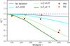Fig. 5 Correlation ratio modelled with Gaussian spatial variations of the polarized dust spectral index, in LR42 as in Fig. 2. The HM and DS Planck measurements are shown as diamonds and squares, respectively. The model is plotted for four values of $\mathrm{\Delta }{\mathit{\delta }}_{\mathrm{d}}^{\mathrm{P}}$, which is defined as the standard deviation of the Gaussian realization of the spectral index after smoothing at 1°. The first model, with $\mathrm{\Delta }{\mathit{\delta }}_{\mathrm{d}}^{\mathrm{P}}\mathrm{=}\mathrm{0}$, is described in Sect. 3.2.

We compare our estimate of the spectral index variations for dust polarization to those measured for the total dust intensity. We use the Commander (Eriksen et al. 2006, 2008) dust component maps derived from a modified blackbody fit to Planck data (Planck Collaboration X 2016), providing two separate maps of dust temperature and dust spectral index. From the ratio I₃₅₃/I₂₁₇ computed from these two maps, we derive an equivalent all-sky map of the intensity dust spectral index, $\begin{array}{c}{\mathrm{˜}}_{}\\ {\mathit{\beta }}_{\mathrm{d}}^{\mathrm{I}}\end{array}$, assuming a constant dust temperature of T_d = 19.6 K. We use the two half-mission maps of the dust spectral index, computed from 1° resolution maps, instead of the full-survey map, in order to reduce the impact of noise and systematic effects when computing the covariance, and we derive an estimate of the standard deviation of the dust spectral index in intensity, $\mathrm{\Delta }{\mathit{\delta }}_{\mathrm{d}}^{\mathrm{I}}\mathrm{\approx }\mathrm{0.045}$ in LR42, about half the value measured for polarization in the same region. We note that this value is not corrected for the contribution of the data noise and the anisotropies of the cosmic infrared background (Planck Collaboration Int. XXII 2015). Both of these contribution are much smaller than the empirical value of 0.17 found in Planck Collaboration Int. XXII (2015), which is dominated by noise.

5.2. Polarization angle variations

In a second approach, we assume that the decorrelation of the BB power spectrum between 217 and 353 GHz can be explained by spatial variations of the polarization angle, keeping the dust temperature and polarized spectral index constant over the whole sky. Unlike the first model, this modelling approach conserves the total power in the power spectrum. It is motivated by the nature of the polarized signal, which can be considered as the sum of spin-2 quantities over multiple components with varying spectral dependencies along the line of sight. Physical interpretation of polarization angle variations are discussed further in Sect. 5.3.

The spatial variations of the polarization angle are assumed to follow a circular normal distribution (or von Mises distribution) around 0, given by $\mathit{f}\mathrm{(}\mathit{\theta }\hspace{0.17em}\mathrm{|}\hspace{0.17em}\mathit{\kappa }\mathrm{)}\mathrm{=}\frac{{\mathrm{e}}^{\mathit{\kappa }\cos \mathrm{\left(}\mathit{\theta }\mathrm{\right)}}}{\mathrm{2}\mathit{\pi }{\mathrm{ℐ}}_{\mathrm{0}}\mathrm{\left(}\mathit{\kappa }\mathrm{\right)}}\mathit{,}$(9)where ℐ₀(x) is the modified Bessel function of order 0, and κ is analogous to 1 /σ² for the normal distribution. While the circular normal distribution allows us to define random angles in the range [− π,π], we re-scale the realizations of angular variations to match the definition for the range of polarization angles lying between −π/ 2 and π/ 2. Again we start from a set of Q and U dust maps at 277 GHz, which are then extrapolated to 217 and 353 GHz following a modified blackbody spectrum using T_d = 19.6 K and ${\mathit{\beta }}_{\mathrm{d}}^{\mathrm{P}}\mathrm{=}\mathrm{1.59}$. The polarization pseudo-vector obtained from Q and U is rotated independently at each frequency using two different realizations of the polarization angle variations. The correlation ratio model is then obtained by averaging 100 realizations of the correlation ratio computed from a pair of simulated maps.

This model is illustrated Fig. 6 for three finite values of κ in the LR42 region. The case κ = 2, which matches the Planck data quite well at ℓ ~ 100, represents a 1 σ dispersion of the polarization angle of about 2° between the 217 and 353 GHz polarization maps, after smoothing at 1° resolution.

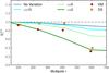Fig. 6 As in Fig. 5, but illustrating the correlation ratio modelled with Gaussian spatial variations of the polarization angle. The model is plotted for four values of κ, which sets the level of the circular normal distribution for the polarization angle, analogous to 1 /σ2 for the normal distribution.

5.3. Origin of the spatial variations of the polarized SED

The spatial variations of the Galactic dust SED are found to be greater for dust polarization than for dust intensity. This difference could result from the lack of correlation between spectral variation and emission features in our modelling in Sect. 5.1. It could also reflect the different nature of the two observables. While variations in the dust SED tend to average out in intensity (because it is a scalar quantity), they may not average out as much in polarization (because it is a pseudo-vector). In other words, dust polarization depends on the magnetic field structure, while dust intensity does not. In this section, we give further details of this interpretation of the decorrelation.

The analysis of Planck data offers several lines of evidence for the imprint of interstellar magneto-hydrodynamical (MHD) turbulence on the dust polarization sky. Firstly, Planck Collaboration Int. XIX (2015) has reported an anti-correlation between the polarization fraction and the local dispersion of the polarization angle. Secondly, large filamentary depolarization patterns observed in the Planck 353 GHz maps are associated, in most cases, with large, local, fluctuations of the polarization angles related to the magnetic field structure (Planck Collaboration Int. XIX 2015). Thirdly, the polarization fraction of the Planck 353 GHz map shows a large scatter at high and intermediate latitudes, which can be interpreted as line of sight depolarization associated with interstellar MHD turbulence (Planck Collaboration Int. XX 2015; Planck Collaboration Int. XLIV 2016). Lastly, several studies have reported a clear trend where the magnetic field is locally aligned with the filamentary structure of interstellar matter (Martin et al. 2015; Clark et al. 2015; Planck Collaboration Int. XXXII 2016; Planck Collaboration Int. XXXVIII 2016; Kalberla et al. 2016).

As presented in Planck Collaboration Int. XLIV (2016), the Planck polarized data at high Galactic latitudes can be modelled using a small number of effective polarization layers in each of which the Galactic magnetic field has a turbulent component of the magnetic field with a distinct orientation. Within this model, the integration of dust polarization along the line of sight can be viewed as the result of an oriented random walk in the (Q, U) plane, with a small number of steps tending towards the mean direction of the Galactic magnetic field. The magnetic field orientation of each turbulent layer sets the direction of the step, while the dust polarization properties, including the efficiency of grain alignment, sets their length. Changes in dust properties generate differences in the relative lengths of the steps across frequency, and thereby differences in the polarization fraction and angle, as illustrated graphically in Fig. 7. In this framework, variations of the dust SED along the line of sight impact both the polarization fraction and the polarization angle, because the structure of the magnetic field and of diffuse interstellar matter are correlated (Planck Collaboration Int. XXXII 2016; Planck Collaboration Int. XXXVIII 2016). In the random walk, the variations in length and angle of the polarization pseudo-vector have the most impact for a small number of steps. Planck Collaboration Int. XLIV (2016) related the number of layers in their model to the density structure of the diffuse interstellar medium and to the correlation length of the turbulent component of the magnetic field along the line of sight.

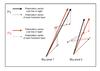Fig. 7 Schematic illustration of the decomposition of the line of sight complex polarization vector (in the (Q, U) space) into a random walk process through four turbulent layers, shown for two neighbouring pixels at two frequencies, ν1 and ν2. The integrated polarization pseudo-vectors are affected by the polarization angle fluctuations, leading to a decorrelation between the two frequencies.

A quantitative modelling of this perspective on dust polarization is required to assess its ability to reproduce the results of our analysis of the Planck data and its impact on the dust/CMB component-separation task. To our knowledge, none of the studies carried out so far to quantify limits set by polarized dust foregrounds on future CMB experiments in order to search for primordial B-modes (except for the work of Tassis & Pavlidou 2015) have considered the frequency decorrelation that arises from the interplay between dust properties and interstellar MHD turbulence.

6. Conclusions

We have used the 217 and 353 GHz Planck 2015 data to investigate the spatial variation of the polarized dust SED at high Galactic latitudes. We computed ${\mathrm{ℛ}}_{\mathit{\ell }}^{\mathit{BB}}$ – the BB cross-spectrum between the Planck polarization maps in these bands divided by the geometric mean of the two auto-spectra in the same bands – over large regions of the sky at high latitudes, for multipoles 50 <ℓ< 700. The value of ${\mathrm{ℛ}}_{\mathit{\ell }}^{\mathit{BB}}$ was computed with distinct sets of data to control systematics.

The ratio ${\mathrm{ℛ}}_{\mathit{\ell }}^{\mathit{BB}}$ has been shown to be significantly lower than what is expected purely from the presence of CMB and noise in the data with a confidence, estimated using data simulations, higher than 99%. We interpret this result as evidence of significant spatial variations of the dust polarization SED.

In the multipole bin 50 <ℓ< 160 that encompasses the recombination bump of the primordial B-mode signal, ${\mathrm{ℛ}}_{\mathit{\ell }}^{\mathit{BB}}$ values are consistent for the distinct Planck data splits we used. The measured values exhibit a systematic trend with column density, where ${\mathrm{ℛ}}_{\mathit{\ell }}^{\mathit{BB}}$ decreases with decreasing mean column densities N_{H i} as 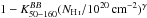$\mathrm{1}\mathrm{-}{\mathit{K}}_{\mathrm{50}\mathrm{-}\mathrm{160}}^{\mathit{BB}}\mathrm{(}{\mathit{N}}_{\mathrm{H}\hspace{0.17em}{i}}\mathit{/}{\mathrm{10}}^{\mathrm{20}}\hspace{0.17em}{\mathrm{cm}}^{-2}{\mathrm{)}}^{\mathit{\gamma }}$, with γ = −1.76 ± 0.69 and ${\mathit{K}}_{\mathrm{50}\mathrm{-}\mathrm{160}}^{\mathit{BB}}\mathrm{=}\mathrm{0.40}\mathrm{\pm }\mathrm{0.32}$. This suggests that, statistically speaking, the cleaner a sky area is from Galactic foregrounds, the more challenging it may be to extrapolate dust polarization from submillimetre to CMB bands.

The spatial variations of the dust SED are shown to be stronger in polarization than in intensity. This difference may reflect the interplay, encoded in the data, between the polarization properties of dust grains, including grain alignment, the Galactic magnetic field, and the density structure of interstellar matter.

We have proposed two toy models to quantify the observed decorrelation, one based on spatial Gaussian variations of the polarized dust spectral index and the other on spatial Gaussian variations of the polarization angle. Both models reproduce the general trend observed in Planck data, with reasonable accuracy given the noise level of the Planck measurements. They represent a first step in characterizing variations of the dust SED, as a prelude to further work on a physically motivated model, which will take into account the expected correlation between the spatial variations of the SED and structures in the dust polarization maps.

Spatial variations of the dust SED can lead to biased estimates of the tensor-to-scalar ratio, r, because of inaccurate extrapolation of dust polarization when cleaning or modelling the B-mode signal at microwave frequencies. As an illustration, we have shown that in a region such as that observed by the BICEP2-Keck Array, a decorrelation of 15% between the 353 and 150 GHz bands could result in a likelihood posterior on the tensor-to-scalar ratio of r = 0.046 ± 0.036, comparable to the joint BICEP2 and Keck Array/Planck Collaboration result.

It appears essential now to place tighter constraints on the spectral dependence of polarized dust emission in the submillimetre in order to properly propagate the information on the Galactic foregrounds into the CMB bands. More specifically, the spatial variations of the polarized dust SED need to be mapped and modelled with improved accuracy in order to be able to confidently reach a level of Galactic dust residual lower than r ~ 10^-2.

Acknowledgments

The Planck Collaboration acknowledges the support of: ESA; CNES, and CNRS/INSU-IN2P3-INP (France); ASI, CNR, and INAF (Italy); NASA and DoE (USA); STFC and UKSA (UK); CSIC, MINECO, J.A., and RES (Spain); Tekes, AoF, and CSC (Finland); DLR and MPG (Germany); CSA (Canada); DTU Space (Denmark); SER/SSO (Switzerland); RCN (Norway); SFI (Ireland); FCT/MCTES (Portugal); ERC and PRACE (EU). A description of the Planck Collaboration and a list of its members, indicating which technical or scientific activities they have been involved in, can be found at http://www.cosmos.esa.int/web/planck/planck-collaboration. The research leading to these results has received funding from the European Research Council under the European Union’s Seventh Framework Programme (FP7/2007-2013)/ERC grant agreement No. 267934.

References

Appendix A: Distribution of the ${\mathrm{ℛ}}_{\mathit{\ell }}^{{BB}}$ from Planck simulations

We present in this appendix the distribution of the ratio ${\mathrm{ℛ}}_{\mathit{\ell }}^{\mathit{BB}}$ for our simulations of the Planck 217 and 353 GHz maps, including Gaussian CMB, dust, and Planck noise, which are described in Sect. 3.3. Since the quantity ${\mathrm{ℛ}}_{\mathit{\ell }}^{\mathit{BB}}$ is a ratio, we expect distributions that are strongly non-Gaussian, even for Gaussian simulations, as soon as the denominator gets close to zero.

In Figs. A.1–A.9, we show the histogram of the ${\mathrm{ℛ}}_{\mathit{\ell }}^{\mathit{BB}}$ correlation ratio from 1000 realizations of detector-set and half-mission simulations. The histogram “occurrences” are the fractions of simulations that fall in each ${\mathrm{ℛ}}_{\mathit{\ell }}^{\mathit{BB}}$ bin. These are compared to the values obtained from the Planck data. Since we compute only noise-independent cross-spectra that can take negative values, when ${\mathrm{ℛ}}_{\mathit{\ell }}^{\mathit{BB}}$ has an imaginary denominator, the data value is absent. The PTE for each data set, computed as the percentage of simulations that have a smaller ${\mathrm{ℛ}}_{\mathit{\ell }}^{\mathit{BB}}$ than the data, is given in Table 1.

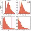Fig. A.1 Distribution of the correlation ratios ${\mathrm{ℛ}}_{\mathit{\ell }}^{\mathit{BB}}$ on the LR16 region from Planck simulations for detector-set (DS, red histograms) and half-mission (HM, orange histograms) data splits, for the four multipole bins we use in the analysis: top left, ℓ ∈ [50,160]; top right, ℓ ∈ [160,320]; bottom left, ℓ ∈ [320,500]; and bottom right, ℓ ∈ [500,700]. The values derived from the data are shown as vertical lines of the corresponding colour. The PTEs corresponding to these data values with respect to the simulations are reported in Table 1.

Fig. A.2 Same as Fig. A.1, for the LR24 region.

Fig. A.3 Same as Fig. A.1, for the LR33 region.

Fig. A.4 Same as Fig. A.1, for the LR42 region.

Fig. A.5 Same as Fig. A.1, for the LR53 region.

Fig. A.6 Same as Fig. A.1, for the LR63N region.

Fig. A.7 Same as Fig. A.1, for the LR63S region.

Fig. A.8 Same as Fig. A.1, for the LR63 region.

Fig. A.9 Same as Fig. A.1, for the LR72 region.

All Tables

All Figures

Fig. 1 Masks and complementary science regions that retain fractional coverage of the sky, fsky, from 0.8 to 0.2 (see details in Sect. 2.2). The grey is the CO mask, whose complement is a selected region with fsky = 0.8. In increments of fsky = 0.1, the retained regions can be identified by the colours from yellow (0.3) to blue (0.8). The LR63N and LR63S regions are displayed in black and white, respectively, and the LR63 region is the union of the two. Also shown is the (unapodized) point source mask used.

In the text

Fig. 2 Dust polarization correlation ratios ${\mathrm{ℛ}}_{\mathit{\ell }}^{\mathit{EE}}$ (top panel) and ${\mathrm{ℛ}}_{\mathit{\ell }}^{\mathit{BB}}$ (bottom panel) between 217 and 353 GHz, computed on the LR63 region. The correlation ratios determined from the detector-set data (DS) splits are shown as yellow squares and the ratios computed from the half-mission (HM) splits as red diamonds. The correlation ratio expectations for the model described in Eq. (5) are shown as blue dashed lines (blue circles when binned as the data). Horizontal blue segments in the top panel represent the range of the ℓ bins. The uncertainties have been estimated as the median absolute deviation over a set of 1000 simulations (see Sect. 2.3) of CMB, dust, and Gaussian noise.

In the text

Fig. 3 Dependence of the Planck correlation ratios with the mean column density of the region on which they are computed in the first multipole bin (ℓ = [50,160]). The HM and DS measurements can be compared to the theoretical expectations (including dust and CMB, as in Eq. (5)) shown as blue segments. The grey bars give the 68% and 95% confidence levels computed over 1000 realizations of dust, CMB, and Gaussian noise. The column density dependence fit by a power law (see Eq. (6)) is shown as a dashed line.

In the text

Fig. 4 ${\mathit{C}}_{\mathit{\ell }}^{\mathit{BB}}$ spectra likelihood posteriors on the r and Ad parameters derived from the simulations of the BICEP2-Keck and Planck 353 GHz data, using: 150 and 353 GHz channels (BKP, red); and 95, 150 and 353 GHz channels (BK(+95), blue). The 1D posteriors of r (marginalized over ${\mathit{\beta }}_{\mathrm{d}}^{\mathrm{P}}$ and Ad) and of Ad (marginalized over ${\mathit{\beta }}_{\mathrm{d}}^{\mathrm{P}}$ and r) are shown in the left and middle panels (blue and red lines, respectively). The input value in our simulations for the dust amplitude at 353 GHz (4.5 μK2 at ℓ = 80) is indicated as a dashed line. The 2D posterior marginalized over ${\mathit{\beta }}_{\mathrm{d}}^{\mathrm{P}}$ is presented in the right panel (68% in darker shading and 95% in lighter shading).

In the text

Fig. 5 Correlation ratio modelled with Gaussian spatial variations of the polarized dust spectral index, in LR42 as in Fig. 2. The HM and DS Planck measurements are shown as diamonds and squares, respectively. The model is plotted for four values of $\mathrm{\Delta }{\mathit{\delta }}_{\mathrm{d}}^{\mathrm{P}}$, which is defined as the standard deviation of the Gaussian realization of the spectral index after smoothing at 1°. The first model, with $\mathrm{\Delta }{\mathit{\delta }}_{\mathrm{d}}^{\mathrm{P}}\mathrm{=}\mathrm{0}$, is described in Sect. 3.2.

In the text

	Fig. 6 As in Fig. 5, but illustrating the correlation ratio modelled with Gaussian spatial variations of the polarization angle. The model is plotted for four values of κ, which sets the level of the circular normal distribution for the polarization angle, analogous to 1 /σ2 for the normal distribution.
In the text

	Fig. 7 Schematic illustration of the decomposition of the line of sight complex polarization vector (in the (Q, U) space) into a random walk process through four turbulent layers, shown for two neighbouring pixels at two frequencies, ν1 and ν2. The integrated polarization pseudo-vectors are affected by the polarization angle fluctuations, leading to a decorrelation between the two frequencies.
In the text

Fig. A.1 Distribution of the correlation ratios ${\mathrm{ℛ}}_{\mathit{\ell }}^{\mathit{BB}}$ on the LR16 region from Planck simulations for detector-set (DS, red histograms) and half-mission (HM, orange histograms) data splits, for the four multipole bins we use in the analysis: top left, ℓ ∈ [50,160]; top right, ℓ ∈ [160,320]; bottom left, ℓ ∈ [320,500]; and bottom right, ℓ ∈ [500,700]. The values derived from the data are shown as vertical lines of the corresponding colour. The PTEs corresponding to these data values with respect to the simulations are reported in Table 1.

In the text

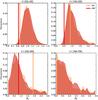	Fig. A.2 Same as Fig. A.1, for the LR24 region.
In the text

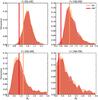	Fig. A.3 Same as Fig. A.1, for the LR33 region.
In the text

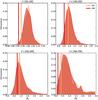	Fig. A.4 Same as Fig. A.1, for the LR42 region.
In the text

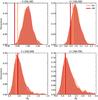	Fig. A.5 Same as Fig. A.1, for the LR53 region.
In the text

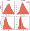	Fig. A.6 Same as Fig. A.1, for the LR63N region.
In the text

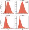	Fig. A.7 Same as Fig. A.1, for the LR63S region.
In the text

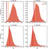	Fig. A.8 Same as Fig. A.1, for the LR63 region.
In the text

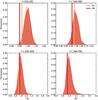	Fig. A.9 Same as Fig. A.1, for the LR72 region.
In the text

References

- Abazajian, K. N., Adshead, P., Ahmed, Z., et al. 2016, ArXiv e-prints [arXiv:1610.02743] [Google Scholar]
- Armitage-Caplan, C., Dunkley, J., Eriksen, H. K., & Dickinson, C. 2012, MNRAS, 424, 1914 [NASA ADS] [CrossRef] [Google Scholar]
- BICEP2 and Keck Array Collaborations 2016, Phys. Rev. Lett., 116, 031302 [NASA ADS] [CrossRef] [PubMed] [Google Scholar]
- BICEP2/Keck Array and Planck Collaborations 2015, Phys. Rev. Lett., 114, 101301 [NASA ADS] [CrossRef] [PubMed] [Google Scholar]
- Choi, S. K., & Page, L. A. 2015, J. Cosmol. Astropart. Phys., 12, 020 [Google Scholar]
- Clark, S. E., Hill, J. C., Peek, J. E. G., Putman, M. E., & Babler, B. L. 2015, Phys. Rev. Lett., 115, 241302 [NASA ADS] [CrossRef] [Google Scholar]
- Creminelli, P., López Nacir, D., Simonović, M., Trevisan, G., & Zaldarriaga, M. 2015, J. Cosmol. Astropart. Phys., 11, 31 [NASA ADS] [CrossRef] [Google Scholar]
- Delabrouille, J., Betoule, M., Melin, J.-B., et al. 2013, A&A, 553, A96 [NASA ADS] [CrossRef] [EDP Sciences] [Google Scholar]
- Eriksen, H. K., Dickinson, C., Lawrence, C. R., et al. 2006, ApJ, 641, 665 [NASA ADS] [CrossRef] [Google Scholar]
- Eriksen, H. K., Jewell, J. B., Dickinson, C., et al. 2008, ApJ, 676, 10 [NASA ADS] [CrossRef] [Google Scholar]
- Errard, J., Feeney, S. M., Peiris, H. V., & Jaffe, A. H. 2016, JCAP, 03, 052 [Google Scholar]
- Górski, K. M., Hivon, E., Banday, A. J., et al. 2005, ApJ, 622, 759 [NASA ADS] [CrossRef] [Google Scholar]
- Kalberla, P. M. W., Kerp, J., Haud, U., et al. 2016, ApJ, 821, 117 [NASA ADS] [CrossRef] [Google Scholar]
- Krachmalnicoff, N., Baccigalupi, C., Aumont, J., Bersanelli, M., & Mennella, A. 2016, A&A, 588, A65 [NASA ADS] [CrossRef] [EDP Sciences] [Google Scholar]
- Martin, P. G., Blagrave, K. P. M., Lockman, F. J., et al. 2015, ApJ, 809, 153 [NASA ADS] [CrossRef] [Google Scholar]
- Planck Collaboration XI. 2014, A&A, 571, A11 [NASA ADS] [CrossRef] [EDP Sciences] [Google Scholar]
- Planck Collaboration I. 2016, A&A, 594, A1 [NASA ADS] [CrossRef] [EDP Sciences] [Google Scholar]
- Planck Collaboration VII. 2016, A&A, 594, A7 [NASA ADS] [CrossRef] [EDP Sciences] [Google Scholar]
- Planck Collaboration VIII. 2016, A&A, 594, A8 [NASA ADS] [CrossRef] [EDP Sciences] [Google Scholar]
- Planck Collaboration X. 2016, A&A, 594, A10 [NASA ADS] [CrossRef] [EDP Sciences] [Google Scholar]
- Planck Collaboration XII. 2016, A&A, 594, A12 [NASA ADS] [CrossRef] [EDP Sciences] [Google Scholar]
- Planck Collaboration XIII. 2016, A&A, 594, A13 [NASA ADS] [CrossRef] [EDP Sciences] [Google Scholar]
- Planck Collaboration XXV. 2016, A&A, 594, A25 [NASA ADS] [CrossRef] [EDP Sciences] [Google Scholar]
- Planck Collaboration Int. XVII. 2014, A&A, 566, A55 [NASA ADS] [CrossRef] [EDP Sciences] [Google Scholar]
- Planck Collaboration Int. XIX. 2015, A&A, 576, A104 [NASA ADS] [CrossRef] [EDP Sciences] [Google Scholar]
- Planck Collaboration Int. XX. 2015, A&A, 576, A105 [NASA ADS] [CrossRef] [EDP Sciences] [Google Scholar]
- Planck Collaboration Int. XXII. 2015, A&A, 576, A107 [NASA ADS] [CrossRef] [EDP Sciences] [Google Scholar]
- Planck Collaboration Int. XXX. 2016, A&A, 586, A133 [NASA ADS] [CrossRef] [EDP Sciences] [Google Scholar]
- Planck Collaboration Int. XXXII. 2016, A&A, 586, A135 [NASA ADS] [CrossRef] [EDP Sciences] [Google Scholar]
- Planck Collaboration Int. XXXVIII. 2016, A&A, 586, A141 [NASA ADS] [CrossRef] [EDP Sciences] [Google Scholar]
- Planck Collaboration Int. XLI. 2016, A&A, 596, A102 [NASA ADS] [CrossRef] [EDP Sciences] [Google Scholar]
- Planck Collaboration Int. XLIV. 2016, A&A, 596, A105 [NASA ADS] [CrossRef] [EDP Sciences] [Google Scholar]
- Planck Collaboration Int. XLVI. 2016, A&A, 596, A107 [NASA ADS] [CrossRef] [EDP Sciences] [Google Scholar]
- Planck Collaboration Int. XLVII. 2016, A&A, 596, A108 [NASA ADS] [CrossRef] [EDP Sciences] [Google Scholar]
- Remazeilles, M., Dickinson, C., Eriksen, H. K. K., & Wehus, I. K. 2016, MNRAS, 458, 2032 [NASA ADS] [CrossRef] [Google Scholar]
- Tassis, K., & Pavlidou, V. 2015, MNRAS, 451, L90 [NASA ADS] [CrossRef] [Google Scholar]
- Tristram, M., Macías-Pérez, J. F., Renault, C., & Santos, D. 2005, MNRAS, 358, 833 [NASA ADS] [CrossRef] [Google Scholar]
- Vansyngel, F., Boulanger, F., Ghosh, T., et al., 2016, A&A, submitted [arXiv:1611.02577] [Google Scholar]
Appendix A: Distribution of the  from Planck simulations