© ESO, 2017

1. Introduction

Simulations of convection-driven dynamos have recently reached a level of sophistication where they capture effects observed in the Sun such as equatorward migration of activity belts (Schrinner et al. 2011; Käpylä et al. 2012; Augustson et al. 2015; Duarte et al. 2016) and irregular cycle variations such as grand minima and long-term modulations (Passos & Charbonneau 2014; Käpylä et al. 2016a). Most of these simulations are individual numerical experiments, and it is not clear how they are situated in parameter space in relation to each other. Important parameters in this connection concern the relative strengths of different diffusion coefficients, viscosity (ν), and magnetic (η) and thermal (χ) diffusivities present in the system. Their ratios are characterized by the thermal and magnetic Prandtl numbers, Pr = ν/χ and Pr_M = ν/η, respectively. In the solar convection zone, these Prandtl numbers are Pr ≪ 1 and Pr_M ≪ 1, while the fluid and magnetic Reynolds numbers, Re = ul/ν and Re_M = ul/η, with u and l being the characteristic velocity and length scale, are on the orders of 10¹² and 10⁹, respectively. Such parameter regimes are not accessible to current numerical simulations, which are restricted to Pr ≈ 1, Pr_M ≈ 1, and Reynolds numbers on the order of 10²−10³. In all simulations by a number of different groups, the dominant contribution to thermal diffusion is made by a subgrid-scale (SGS) coefficient χ_SGS whose magnitude is much higher than the radiative one. Similar arguments also apply to ν and η, but since the functional form of these diffusion operators is unchanged, we omit the subscript SGS in them. Thus, the relevant thermal Prandtl number in simulations is Pr_SGS = ν/χ_SGS. We emphasize that this applies to simulations of all groups, although the nomenclature may be different (see Table A.1). This is also true for groups using realistic luminosities, and thus the correct order of magnitude for the radiative diffusivity (e.g., Brun et al. 2004; Hotta et al. 2016).

When the convection simulations of Käpylä et al. (2012) in wedge geometry showed clear equatorward migration for the first time, it was not obvious that this was related to their choice of Pr_SGS = 2.5 compared with Pr_SGS ≲ 1 used in most earlier simulations that showed either quasi-stationary configurations (Brown et al. 2010) or either weak or poleward migration (e.g., Ghizaru et al. 2010; Käpylä et al. 2010b; Brown et al. 2011; Gastine et al. 2012). Recently, Warnecke et al. (2014) showed that the change in the dynamo behavior between Pr_SGS> 1 and Pr_SGS< 1 regimes is due to a change in the differential rotation profile, which in the Pr_SGS ≳ 1 regime leads to a region of negative radial shear that facilitates the equatorward migration. The magnetic Prandtl number, which is proportional to the magnetic Reynolds number, can also strongly affect the results. Increasing Re_M by increasing Pr_M can allow magnetohydrodynamic (MHD) instabilities such as magnetic buoyancy (Parker 1955) and magnetorotational instabilities (e.g., Parfrey & Menou 2007; Masada 2011) to be excited.

Increasing the magnetic Reynolds number can influence the large-scale dynamo by several other avenues. First, the most easily excited dynamo mode can change. Second, a small-scale dynamo is most likely excited after Re_M exceeds a threshold value (e.g., Cattaneo 1999), and this may also affect the large-scale dynamo by modifying the velocity field. Third, Boussinesq simulations indicate that differential rotation is strongly quenched as the magnetic Reynolds number increases (Schrinner et al. 2012). This was shown to be associated with a transition from oscillatory multipolar large-scale field configurations to quasi-stationary dipole-dominated dynamos as a function of Re_M. One of the main goals of the present paper is therefore to systematically study the effects of varying Prandtl numbers on the differential rotation and dynamo modes excited in the simulations. We note that similar parameter studies have been performed with Boussinesq simulations (e.g., Simitev & Busse 2005; Busse & Simitev 2006). Here we explore the stratified, fully compressible simulations and reach parameter regimes that are significantly more supercritical in terms of both the convection and the dynamo.

Another important aspect is related to the saturation level of the large-scale field in simulations at high Re_M. Dynamo theory experienced a crisis in the early 1990s when it was discovered that the energy of the large-scale magnetic field saturates at a level that is inversely proportional to the magnetic Reynolds number (Gruzinov & Diamond 1995; Brandenburg & Dobler 2001). If this were to carry over to the Sun, where the magnetic Reynolds number is on the order of 10⁹ or greater, only very weak large-scale fields would survive. This phenomenon was related to a catastrophic quenching of the α effect (Cattaneo & Vainshtein 1991; Vainshtein & Cattaneo 1992; Cattaneo & Hughes 1996).

Later, this was understood in terms of magnetic helicity: if the system is closed or fully periodic, that is, when magnetic field lines do not cross the boundary of the system, no flux of magnetic helicity in or out can occur, and only the molecular diffusion can change it (Brandenburg 2001). In astrophysical systems this would mean that magnetic helicity would be nearly conserved. However, astrophysical systems are not closed and magnetic helicity can escape, for example, through coronal mass ejections in the Sun (e.g., Blackman & Brandenburg 2003; Warnecke et al. 2011, 2012) or through winds from galaxies (Shukurov et al. 2006; Sur et al. 2007; Del Sordo et al. 2013). In mean-field theory these physical effects are parameterized by fluxes, which lead to alleviation of catastrophic quenching in suitable parameter regimes (e.g., Brandenburg et al. 2009).

Direct numerical simulations of large-scale dynamos have demonstrated that open boundaries lead to alleviation of catastrophic quenching in accordance with the interpretation in terms of magnetic helicity conservation (e.g., Brandenburg & Sandin 2004; Käpylä et al. 2010a). Although the large-scale magnetic field amplitude does not decrease proportional to Re_M in the cases when open boundaries are used, there is still a decreasing trend even at the highest currently studied Re_M in local simulations of convection-driven dynamos (e.g., Käpylä et al. 2010a). This, however, is compatible with mean-field models, which suggest that the magnetic helicity fluxes become effective only at significantly higher Re_M (Brandenburg et al. 2009; Del Sordo et al. 2013).

In convective dynamos in spherical coordinates the computational challenge is even greater and systematic parameter scans have not been performed. Some preliminary attempts have been made, but the results remain inconclusive. An illuminating example is the study of Nelson et al. (2013), where the large-scale axisymmetric field decreases by a factor of two when the magnetic Reynolds number is increased by a factor of four, which is still rather steep. In a recent paper, Hotta et al. (2016) showed that in even higher-Re_M simulations the mean magnetic energy recovers, and the authors claim that this is a consequence of an efficient small-scale dynamo that suppresses small-scale flows. Another goal of the present paper is therefore to study the saturation level of the large-scale field in convection-driven dynamos in spherical coordinates with and without a simultaneous small-scale dynamo (hereafter SSD).

In the present study, we employ a spherical wedge geometry by imposing either a perfect conductor or a normal field boundary condition at high latitudes. Earlier mean-field simulations of αΩ dynamos have suggested that solutions with a perfect conductor boundary condition are similar to those in full spherical shells (Jennings et al. 1990). However, more recent work by Cole et al. (2016) has demonstrated that this conclusion is not generally valid and depends on the nature of the solutions. Their work also suggests that the use of a normal field boundary condition at high latitudes might be a better way of obtaining solutions that are applicable to full spherical shells. Owing to this uncertainty, we investigate here cases with both types of boundary conditions.

2. Model

Our model is similar to that of Käpylä et al. (2012) and is described in detail in Käpylä et al. (2013). The model describes the dynamics of magnetized gas in spherical coordinates where only parts of the latitude and longitude ranges are retained. More specifically, the model covers a wedge that spans r₀ ≤ r ≤ r₁ in radius, θ₀ ≤ θ ≤ π−θ₀ in colatitude, and 0 ≤ φ ≤ φ₀ in longitude. Here we use r₀ = 0.7 R_⊙, r₁ = R_⊙, and where R_⊙ = 6.96 × 10⁸ m is the solar radius, θ₀ = 15°, and φ₀ = 90°.

We solve the following set of compressible hydromagnetics equations $\begin{array}{ccc}& & \frac{\mathit{\partial }{A}}{\mathit{\partial t}}\mathrm{=}{U}\mathrm{\times }{B}\mathrm{-}\mathit{\eta }{\mathit{\mu }}_{\mathrm{0}}{J}\mathit{,}\\ & & \frac{\mathit{D}\ln \mathit{\rho }}{\mathit{Dt}}\mathrm{=}\mathrm{-}{\nabla }{·}{U}\mathit{,}\\ & & \frac{\mathit{D}{U}}{\mathit{Dt}}\mathrm{=}{g}\mathrm{-}\mathrm{2}{{\Omega }}_{\mathrm{0}}\mathrm{\times }{U}\mathrm{+}\frac{\mathrm{1}}{\mathit{\rho }}\mathrm{[}{\nabla }{·}\mathrm{(}\mathrm{2}\mathit{\nu \rho }{S}\mathrm{)}\mathrm{-}{\nabla }\mathit{p}\mathrm{+}{J}\mathrm{\times }{B}\mathrm{]}\mathit{,}\\ & & \end{array}$where A is the magnetic vector potential, U is the velocity, B = ∇ × A is the magnetic field, η is the magnetic diffusivity, μ₀ is the permeability of vacuum, J = ∇ × B/μ₀ is the current density, D/Dt = ∂/∂t + U·∇ is the advective time derivative, ρ is the density, g is the acceleration due to gravity, and Ω₀ = (cosθ,−sinθ,0)Ω₀ is the angular velocity vector where Ω₀ is the rotation rate of the frame of reference, ν is the kinematic viscosity, p is the pressure, and s is the specific entropy with Ds = c_VDlnp−c_PDlnρ. The gas is assumed to obey the ideal gas law, p = (γ−1)ρe, where e = c_VT is the specific internal energy and γ = c_P/c_V is the ratio of specific heats at constant pressure and volume, respectively. The rate of strain tensor is given by 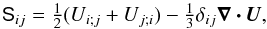$\begin{array}{ccc}{\mathrm{S}}_{\mathit{ij}}\mathrm{=}\frac{\mathrm{1}}{\mathrm{2}}\mathrm{(}{\mathit{U}}_{\mathit{i}\mathrm{;}\mathit{j}}\mathrm{+}{\mathit{U}}_{\mathit{j}\mathrm{;}\mathit{i}}\mathrm{)}\mathrm{-}\frac{\mathrm{1}}{\mathrm{3}}{\mathit{\delta }}_{\mathit{ij}}{\nabla }{·}{U}\mathit{,}& & \end{array}$(5)where the semicolons refer to covariant derivatives; see Mitra et al. (2009). The radiative and SGS fluxes are given by $\begin{array}{ccc}{{F}}^{\mathrm{rad}}\mathrm{=}\mathrm{-}\mathit{K}{\nabla }\mathit{T,}{{F}}^{\mathrm{SGS}}\mathrm{=}\mathrm{-}{\mathit{\chi }}_{\mathrm{SGS}}\mathit{\rho T}{\nabla }\mathit{s,}& & \end{array}$(6)where K = c_Pρχ is the heat conductivity, and χ_SGS is the (turbulent) SGS diffusion coefficient for the entropy.

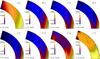Fig. 1 Top row: temporally averaged rotation profiles from Runs A3, B3, C3, and D3 with PrM = 1 and PrSGS varying from 0.25 (left) to 2 (right). Lower row: same as above, but for Runs C2, C3, C4, and C5 with PrSGS = 1 and PrM varying from 0.5 (left) to 5 (right).

2.1. Initial and boundary conditions

We follow the description given in Käpylä et al. (2014) to transform our results into physical units. As our equations are fully compressible, we cannot afford to use the solar luminosity, which would lead to the sound speed dominating the time step. Thus we increase the luminosity substantially, and to compensate for this, we increase the rotation rate to achieve the same rotational influence as in the Sun. Assuming a scaling of the luminosity with the convective energy flux as L ∝ ρu³, we find that the convective velocities increase to one-third power of the luminosity (e.g., Brandenburg et al. 2005; Karak et al. 2015). The ratio between model and solar luminosities is L₀/L_⊙ ≈ 6.4 × 10⁵ in the current simulations. We correspondingly increase the rotation rate by a factor of $\mathrm{(}{\mathit{L}}_{\mathrm{0}}\mathit{/}{\mathit{L}}_{\mathrm{\odot }}{\mathrm{)}}^{\frac{\mathrm{1}}{\mathrm{3}}}\mathrm{\approx }\mathrm{86}$ for the solar case. We reiterate that the main effect of increasing the luminosity is to increase the Mach number and bring the acoustic and dynamical timescales closer to each other, which facilitates the computations with a fully compressible method (cf. Fig. 1 of Käpylä et al. 2013). Another possibility would be to apply the so-called reduced sound speed method where the sound speed is artificially changed so that the Mach number does not become too small at the base of the convection zone (Hotta et al. 2012; Käpylä et al. 2016b).

The higher luminosity also helps to reach a thermal equilibrium within reasonable simulation running time. Furthermore, we assume that the density and the temperature at the base of the convection zone are the same as in the Sun, that is, ρ_bot = 200 kg m^-3 and T = 2.23 × 10⁶ K.

As the initial condition for the hydrodynamics we use an isentropic atmosphere. The temperature gradient is given by $\frac{\mathit{\partial T}}{\mathit{\partial r}}\mathrm{=}\mathrm{-}\frac{\mathit{G}{\mathit{M}}_{\mathrm{\odot }}\mathit{/}{\mathit{r}}^{\mathrm{2}}}{{\mathit{c}}_{\mathrm{V}}\mathrm{(}\mathit{\gamma }\mathrm{-}\mathrm{1}\mathrm{)}\mathrm{(}{\mathit{n}}_{\mathrm{ad}}\mathrm{-}\mathrm{1}\mathrm{)}}\mathit{,}$(7)where G = 6.67 × 10^-11 N m² kg^-2 is Newton’s gravitational constant, M_⊙ = 1.989 × 10³⁰ kg is the solar mass, and n_ad = 1.5 is the polytropic index for an adiabatic stratification.

The initial state is not in thermal equilibrium but closer to the final convecting state to reduce the time needed to reach a statistically stationary state. The heat conductivity has a profile given by K(r) = K₀ [n(r) + 1], where n(r) = δn(r/r₀)¹⁵ + n_ad−δn, with ${\mathit{K}}_{\mathrm{0}}\mathrm{=}\mathrm{(}\mathrm{ℒ}\mathit{/}\mathrm{4}\mathit{\pi }\mathrm{)}{\mathit{c}}_{\mathrm{V}}\mathrm{(}\mathit{\gamma }\mathrm{-}\mathrm{1}\mathrm{)}\mathrm{(}{\mathit{n}}_{\mathrm{ad}}\mathrm{+}\mathrm{1}\mathrm{)}{\mathit{\rho }}_{\mathrm{bot}}\sqrt{\mathit{G}{\mathit{M}}_{\mathrm{\odot }}\hspace{0.17em}{\mathit{R}}_{\mathrm{\odot }}}$, and where ℒ is a dimensionless luminosity defined below. We keep δn = 1.9 fixed in our simulations, resulting a situation where radiation transports all of the flux into the domain, but its contribution diminishes rapidly toward the surface (see, e.g., Fig. 2 of Käpylä et al. 2011a).

The SGS diffusivity χ_SGS for the entropy has a piecewise constant profile, such that the value χ_SGS = 6.1 × 10⁸ m s^-2 is fixed above r = 0.98 R_⊙ in all runs, and the value ${\mathit{\chi }}_{\mathrm{SGS}}^{\mathrm{m}}\mathrm{=}{\mathit{\chi }}_{\mathrm{SGS}}\mathrm{(}\mathit{r}\mathrm{=}{\mathit{r}}_{\mathit{m}}\mathrm{=}\mathrm{0.85}\hspace{0.17em}{\mathit{R}}_{\mathrm{\odot }}\mathrm{)}$ in the bulk of the convection zone is varied by the corresponding Prandtl number (see below). The value below r = 0.75 R_⊙ is set equal to $\mathrm{0.1}{\mathit{\chi }}_{\mathrm{SGS}}^{\mathrm{m}}$. The constant values in the different layers connect smoothly over a transition depth of d = 0.01 R_⊙.

The boundary conditions for the flow are assumed to be impenetrable and stress free, that is, $\begin{array}{ccc}& & {\mathit{U}}_{\mathit{r}}\mathrm{=}\mathrm{0}\mathit{,} \frac{\mathit{\partial }{\mathit{U}}_{\mathit{\theta }}}{\mathit{\partial r}}\mathrm{=}\frac{{\mathit{U}}_{\mathit{\theta }}}{\mathit{r}}\mathit{,} \frac{\mathit{\partial }{\mathit{U}}_{\mathit{\phi }}}{\mathit{\partial r}}\mathrm{=}\frac{{\mathit{U}}_{\mathit{\phi }}}{\mathit{r}} \mathrm{(}\mathit{r}\mathrm{=}{\mathit{r}}_{\mathrm{0}}\mathit{,}{\mathit{r}}_{\mathrm{1}}\mathrm{)}\mathit{,}\\ & & \frac{\mathit{\partial }{\mathit{U}}_{\mathit{r}}}{\mathit{\partial \theta }}\mathrm{=}{\mathit{U}}_{\mathit{\theta }}\mathrm{=}\mathrm{0}\mathit{,} \frac{\mathit{\partial }{\mathit{U}}_{\mathit{\phi }}}{\mathit{\partial \theta }}\mathrm{=}{\mathit{U}}_{\mathit{\phi }}\cot \mathit{\theta } \mathrm{(}\mathit{\theta }\mathrm{=}{\mathit{\theta }}_{\mathrm{0}}\mathit{,\pi }\mathrm{-}{\mathit{\theta }}_{\mathrm{0}}\mathrm{)}\mathit{.} \end{array}$The lower radial boundary is assumed to be perfectly conducting, and on the outer radial boundary the field is purely radial. The latitudinal boundaries are either perfectly conducting (PC) or a normal field (NF) condition is assumed. In terms of the magnetic vector potential, these are given by 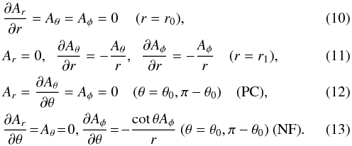$\begin{array}{ccc}& & \frac{\mathit{\partial }{\mathit{A}}_{\mathit{r}}}{\mathit{\partial r}}\mathrm{=}{\mathit{A}}_{\mathit{\theta }}\mathrm{=}{\mathit{A}}_{\mathit{\phi }}\mathrm{=}\mathrm{0}\hspace{0.17em} \mathrm{(}\mathit{r}\mathrm{=}{\mathit{r}}_{\mathrm{0}}\mathrm{)}\mathit{,}\\ & & {\mathit{A}}_{\mathit{r}}\mathrm{=}\mathrm{0}\mathit{,}\frac{\mathit{\partial }{\mathit{A}}_{\mathit{\theta }}}{\mathit{\partial r}}\mathrm{=}\mathrm{-}\frac{{\mathit{A}}_{\mathit{\theta }}}{\mathit{r}}\mathit{,}\frac{\mathit{\partial }{\mathit{A}}_{\mathit{\phi }}}{\mathit{\partial r}}\mathrm{=}\mathrm{-}\frac{{\mathit{A}}_{\mathit{\phi }}}{\mathit{r}} \mathrm{(}\mathit{r}\mathrm{=}{\mathit{r}}_{\mathrm{1}}\mathrm{)}\mathit{,} \\ & & {\mathit{A}}_{\mathit{r}}\mathrm{=}\frac{\mathit{\partial }{\mathit{A}}_{\mathit{\theta }}}{\mathit{\partial \theta }}\mathrm{=}{\mathit{A}}_{\mathit{\phi }}\mathrm{=}\mathrm{0} \mathrm{(}\mathit{\theta }\mathrm{=}{\mathit{\theta }}_{\mathrm{0}}\mathit{,\pi }\mathrm{-}{\mathit{\theta }}_{\mathrm{0}}\mathrm{)} \mathrm{\left(}\mathrm{PC}\mathrm{\right)}\mathit{,}\\ & & \frac{\mathit{\partial }{\mathit{A}}_{\mathit{r}}}{\mathit{\partial \theta }}\mathrm{=}{\mathit{A}}_{\mathit{\theta }}\mathrm{=}\mathrm{0}\mathit{,}\frac{\mathit{\partial }{\mathit{A}}_{\mathit{\phi }}}{\mathit{\partial \theta }}\mathrm{=}\mathrm{-}\frac{\cot \mathit{\theta }{\mathit{A}}_{\mathit{\phi }}}{\mathit{r}}\mathrm{(}\mathit{\theta }\mathrm{=}{\mathit{\theta }}_{\mathrm{0}}\mathit{,\pi }\mathrm{-}{\mathit{\theta }}_{\mathrm{0}}\mathrm{)}\mathrm{\left(}\mathrm{NF}\mathrm{\right)}\mathit{.}\end{array}$For the density and specific entropy we assume vanishing first derivatives on the latitudinal boundaries.

At the lower boundary we specify ${\mathit{F}}_{\mathit{r}}^{\mathrm{rad}}\mathrm{+}{\mathit{F}}_{\mathit{r}}^{\mathrm{SGS}}\mathrm{=}\frac{{\mathit{L}}_{\mathrm{0}}}{\mathrm{4}\mathit{\pi }{\mathit{r}}_{\mathrm{0}}^{\mathrm{2}}}\mathit{,}$(14)which leads to constant input luminosity into the system. On the outer radial boundary we apply a radiative boundary condition $\mathit{\sigma }{\mathit{T}}^{\mathrm{4}}\mathrm{=}{\mathit{F}}_{\mathit{r}}^{\mathrm{rad}}\mathrm{+}{\mathit{F}}_{\mathit{r}}^{\mathrm{SGS}}\mathit{,}$(15)where σ is the Stefan-Boltzmann constant. We use a modified value for σ that takes into account that the luminosity and the temperature at the surface are higher than in the Sun. The value of σ is chosen so that the surface flux, σT⁴, carries the total luminosity through the boundary in the initial non-convecting state.

2.2. System parameters and diagnostics quantities

The parameters governing our models are the dimensionless luminosity $\mathrm{ℒ}\mathrm{=}\frac{{\mathit{L}}_{\mathrm{0}}}{{\mathit{\rho }}_{\mathrm{0}}\mathrm{(}\mathit{G}{\mathit{M}}_{\mathrm{\odot }}{\mathrm{)}}^{\mathrm{3}\mathit{/}\mathrm{2}}\hspace{0.17em}{\mathit{R}}_{\mathrm{\odot }}^{\mathrm{1}\mathit{/}\mathrm{2}}}\mathit{,}$(16)the normalized pressure scale height at the surface, $\mathit{\xi }\mathrm{=}\frac{\mathrm{(}\mathit{\gamma }\mathrm{-}\mathrm{1}\mathrm{)}{\mathit{c}}_{\mathrm{V}}{\mathit{T}}_{\mathrm{1}}}{\mathit{G}{\mathit{M}}_{\mathrm{\odot }}\mathit{/}{\mathit{R}}_{\mathrm{\odot }}}\mathit{,}$(17)with T₁ being the temperature at the surface in the initial state, the Taylor number $\mathrm{Ta}\mathrm{=}\mathrm{(}\mathrm{2}{\mathrm{\Omega }}_{\mathrm{0}}\mathrm{\Delta }{\mathit{r}}^{\mathrm{2}}\mathit{/}\mathit{\nu }{\mathrm{)}}^{\mathrm{2}}\mathit{,}$(18)where Δr = r₁−r₀ = 0.3 R_⊙, as well as the fluid, SGS, and magnetic Prandtl numbers $\mathrm{Pr}\mathrm{=}\frac{\mathit{\nu }}{{\mathit{\chi }}_{\mathrm{m}}}\mathit{,} {\mathrm{Pr}}_{\mathrm{SGS}}\mathrm{=}\frac{\mathit{\nu }}{{\mathit{\chi }}_{\mathrm{SGS}}^{\mathrm{m}}}\mathit{,} {\mathrm{Pr}}_{\mathrm{M}}\mathrm{=}\frac{\mathit{\nu }}{\mathit{\eta }}\mathit{,}$(19)where χ_m = K(r_m) /c_Pρ_m is the thermal diffusivity and ρ_m is the density, both evaluated at r = r_m. We keep Pr = 71.7 fixed and vary Pr_SGS and Pr_M in most of our models, with the exception of Set G, where Pr_SGS and Pr_M are set to unity and Pr is varied by changing the value of ν (see Table 1). The Rayleigh number is defined as $\mathrm{Ra}\mathrm{=}\frac{\mathit{G}{\mathit{M}}_{\mathrm{\odot }}\mathrm{(}\mathrm{\Delta }\mathit{r}{\mathrm{)}}^{\mathrm{4}}}{\mathit{\nu }{\mathit{\chi }}_{\mathrm{SGS}}^{\mathrm{m}}{\mathit{R}}_{\mathrm{\odot }}^{\mathrm{2}}}(\mathrm{-}\frac{\mathrm{1}}{{\mathit{c}}_{\mathrm{P}}}\frac{\mathrm{d}{\mathit{s}}_{\mathrm{hs}}}{\mathrm{d}\mathit{r}}{)}_{{\mathit{r}}_{\mathrm{m}}}\mathit{,}$(20)where s_hs is the entropy in the hydrostatic (hs), non-convecting state obtained from a one-dimensional model where no convection can develop with the prescriptions of K and χ_SGS given above.

The remaining parameters are used only as diagnostics. These include the fluid and magnetic Reynolds numbers, and the Péclet number $\mathrm{Re}\mathrm{=}\frac{{\mathit{u}}_{\mathrm{rms}}}{\mathit{\nu }{\mathit{k}}_{\mathrm{f}}}\mathit{,} {\mathrm{Re}}_{\mathrm{M}}\mathrm{=}\frac{{\mathit{u}}_{\mathrm{rms}}}{\mathit{\eta }{\mathit{k}}_{\mathrm{f}}}\mathit{,} \mathrm{Pe}\mathrm{=}\frac{{\mathit{u}}_{\mathrm{rms}}}{{\mathit{\chi }}_{\mathrm{SGS}}^{\mathrm{m}}{\mathit{k}}_{\mathrm{f}}}\mathit{,}$(21)where ${\mathit{k}}_{\mathrm{f}}\mathrm{=}\mathrm{2}\mathit{\pi }\mathit{/}\mathrm{\Delta }\mathit{r}\mathrm{\approx }\mathrm{21}\hspace{0.17em}{\mathit{R}}_{\mathrm{\odot }}^{-1}$ is an estimate of the wavenumber of the largest eddies. Rotational influence on the flow is given by the Coriolis number $\mathrm{Co}\mathrm{=}\frac{\mathrm{2}{\mathrm{\Omega }}_{\mathrm{0}}}{{\mathit{u}}_{\mathrm{rms}}{\mathit{k}}_{\mathrm{f}}}\mathit{,}$(22)where ${\mathit{u}}_{\mathrm{rms}}\mathrm{=}\sqrt{\mathrm{(}\mathrm{3}\mathit{/}\mathrm{2}\mathrm{)}\mathrm{⟨}{\mathit{U}}_{\mathit{r}}^{\mathrm{2}}\mathrm{+}{\mathit{U}}_{\mathit{\theta }}^{\mathrm{2}}{\mathrm{⟩}}_{\mathit{r\theta \phi t}}}$ is the rms velocity and the subscripts indicate averaging over r, θ, φ, and a time interval during which the run is thermally relaxed. We omit the contribution from the azimuthal velocity in u_rms because it is dominated by differential rotation (Käpylä et al. 2011b).

We define mean quantities as averages over the φ-coordinate and denote them by overbars. We also often average the data in time over the period of the simulations where thermal energy, differential rotation, and large-scale magnetic fields have reached statistically saturated states.

The simulations are performed with the Pencil Code¹, which uses a high-order finite difference method for solving the compressible equations of magnetohydrodynamics.

3. Data analysis: D² statistic

To detect possible cycles and to estimate their average lengths, we have chosen to use D² phase dispersion statistic (Pelt 1983). It has recently been applied to irregularly spaced long-term photometry of solar-like stars (Lindborg et al. 2013; Olspert et al. 2015) as well as to more regularly sampled magnetoconvection simulation data (Karak et al. 2015; Käpylä et al. 2016a). In the previous applications the statistic has been used exclusively on one-dimensional time series (e.g., by fixing a certain latitude and radius in the azimuthally averaged data). In the current study we use a generalized form of the statistic given by 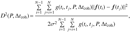${\mathit{D}}^{\mathrm{2}}\mathrm{\left(}\mathit{P,}\mathrm{\Delta }{\mathit{t}}_{\mathrm{coh}}\mathrm{\right)}\mathrm{=}\frac{\sum _{\mathit{i}\mathrm{=}\mathrm{1}}^{\mathit{N}\mathrm{-}\mathrm{1}}\sum _{\mathit{j}\mathrm{=}\mathit{i}\mathrm{+}\mathrm{1}}^{\mathit{N}}\mathit{g}\mathrm{(}{\mathit{t}}_{\mathit{i}}\mathit{,}{\mathit{t}}_{\mathit{j}}\mathit{,P,}\mathrm{\Delta }{\mathit{t}}_{\mathrm{coh}}\mathrm{\left)}\mathrm{\right|}\mathrm{\left|}{f}\mathrm{\right(}{\mathit{t}}_{\mathit{i}}\mathrm{)}\mathrm{-}{f}\mathrm{(}{\mathit{t}}_{\mathit{j}}\mathrm{\left)}\mathrm{\right|}{\mathrm{|}}^{\mathrm{2}}}{\mathrm{2}{\mathit{\sigma }}^{\mathrm{2}}\sum _{\mathit{i}\mathrm{=}\mathrm{1}}^{\mathit{N}\mathrm{-}\mathrm{1}}\sum _{\mathit{j}\mathrm{=}\mathit{i}\mathrm{+}\mathrm{1}}^{\mathit{N}}\mathit{g}\mathrm{(}{\mathit{t}}_{\mathit{i}}\mathit{,}{\mathit{t}}_{\mathit{j}}\mathit{,P,}\mathrm{\Delta }{\mathit{t}}_{\mathrm{coh}}\mathrm{)}}\mathit{,}$(23)where f(t_i) is the vector of observed variables at time moment t_i, σ² = N^-2 ∑ _i,j>i | | f(t_i)−f(t_j) | | ² is the variance of the full time series, g(t_i,t_j,P,Δt_coh) is the selection function, which is significantly greater than zero only when $\begin{array}{ccc}{\mathit{t}}_{\mathit{j}}\mathrm{-}{\mathit{t}}_{\mathit{i}}& \mathrm{\approx }& \mathit{kP,k}\mathrm{=}\mathrm{\pm }\mathrm{1}\mathit{,}\mathrm{\pm }\mathrm{2}\mathit{,}\mathit{...}\mathit{,} \mathrm{and}\\ \left|{\mathit{t}}_{\mathit{j}}\mathrm{-}{\mathit{t}}_{\mathit{i}}\right|& ⪅& \mathrm{\Delta }{\mathit{t}}_{\mathrm{coh}}\mathrm{=}{\mathit{l}}_{\mathrm{coh}}\mathit{P,}\end{array}$where P is the trial period and Δt_coh is the so-called coherence time, which is the measure of the width of the sliding time window wherein the data points are taken into account by the statistic. The number of trial periods fitting into this interval, l_coh = Δt_coh/P, is called the coherence length. With this definition there is no restriction on the dimensionality of the data, but Eq. (23) leaves open the choice of the vector norm. In most cases it is natural to use the Euclidean norm, which we also assume in our analysis. In the following we use this statistic to analyze the radial and azimuthal components of the magnetic field at regions near the surface over latitude intervals, where the cycles are the most pronounced (see Sect. 4.2.2).

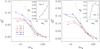Fig. 2 Estimates of radial and latitudinal differential rotation ${\mathrm{\Delta }}_{\mathrm{\Omega }}^{\mathrm{\left(}\mathit{r}\mathrm{\right)}}$ and ${\mathrm{\Delta }}_{\mathrm{\Omega }}^{\mathrm{\left(}\mathit{\theta }\mathrm{\right)}}$, respectively, according to Eq. (26) for Sets A–F as indicated by the legend.

4. Results

We performed six sets of simulations (Sets A–F), each with a constant value of Pr_SGS but changing Pr_M in the range 0.25 ≤ Pr_M ≤ 5; see Table 1. Furthermore, in an additional Set G we fixed Pr_SGS = Pr_M = 1 and varied the Reynolds and Péclet numbers. The rotation rate was varied such that Sets A–D and G have Ω₀ = 5Ω_⊙, whereas in Sets E and F we used 3Ω_⊙ and Ω_⊙, respectively. Sets E and F were included to study the reliability of our findings at slower rotation. In some sets (A, D, E, and F) numerical problems prevented us from using Pr_M = 5. In these cases we used a lower value that produces numerically stable solutions. The latitudinal PC boundary conditions led to numerical problems as a result of an unidentified instability at high magnetic Reynolds numbers near the latitudinal boundaries. Cases where this occurred were rerun with the NF conditions. We did not find major qualitative differences in the behavior of the large-scale field between PC and NF runs with otherwise identical parameters. In the following, we omit the Pr_M = 0.25 runs that did not lead to dynamos in Sets E and F. We note that Run B2 has been presented as Run II in Warnecke et al. (2014), Run D3 as Run A1 in Warnecke et al. (2016a,b), and Run C3 covers the first 120 yr of the run presented in Käpylä et al. (2016a). Furthermore, runs similar to Run D3 (but with Pr_M = 2.5 instead of 2.0) are presented as Runs B4m and C1 in Käpylä et al. (2012, 2013).

4.1. Large-scale flows and their generators

4.1.1. Differential rotation and meridional circulation

The sign of the radial gradient of Ω plays a crucial role in determining the propagation direction of dynamo waves in αΩ dynamos: with a positive α effect in the northern hemisphere, a negative radial gradient of Ω is required to obtain solar-like equatorward migration and vice versa (Parker 1955; Yoshimura 1975). It is remarkable that this rule also seems to apply to the fully nonlinear convective dynamo simulations (Warnecke et al. 2014, 2016b). The current simulations can produce equatorward migration only in cases where a region with a negative radial gradient of Ω occurs at mid-latitudes (e.g., Käpylä et al. 2012, 2013; Augustson et al. 2015) or if the sign of the kinetic helicity, which is a proxy of the α effect, is inverted in the bulk of the convection zone (Duarte et al. 2016).

The simulations of Käpylä et al. (2012), Augustson et al. (2015), Käpylä et al. (2016a), and Warnecke et al. (2016a) showing equatorward migration and a region of negative radial shear at mid-latitudes have Pr_SGS ≳ 1. This is in contrast to earlier simulations with Pr_SGS< 1, which did not show equatorward migration (e.g., Brun et al. 2004; Brown et al. 2011; Nelson et al. 2013) and had consistently positive gradients of Ω. Given that the dynamo wave propagation is apparently heavily influenced by this, it is important to study the effect that Pr_SGS has on the rotation profiles.

We show representative results of the temporally averaged rotation profiles as a function of Pr_SGS from Runs A3, B3, C3, and D3 in the top row of Fig. 1. In the lowest SGS Prandtl number case (Run A3), the angular velocity $\mathrm{\Omega }\mathrm{=}{\mathrm{\Omega }}_{\mathrm{0}}\mathrm{+}{\overline{\mathit{U}}}_{\mathit{\phi }}\mathit{/}\mathit{r}\sin \mathit{\theta }$ decreases monotonically from the equator toward the poles. Much of the latitudinal variation occurs at high latitudes near the latitudinal boundaries. However, the rotation profile is qualitatively similar to those obtained from low Pr_SGS models in fully spherical shells (e.g., Brun et al. 2004; Brown et al. 2010). In Run B3, a dip at mid-latitudes is developing, which is seen to deepen in the higher Pr_SGS Runs C3 and D3. We note that a similar transition occurs also when the density stratification is increased with Pr_SGS = 2...5 (Käpylä et al. 2011a, 2013). The overall magnitude of the differential rotation also decreases from low to high SGS Prandtl numbers. However, much of this variation occurs already between Runs A3 and B3, whereas the differences between Runs B3, C3, and D3 are much smaller.

The time-averaged rotation profiles from runs with Pr_SGS = 1 with varying Pr_M are shown in the lower row of Fig. 1 from Runs C2–C5. The absolute shear decreases steeply as Pr_M and Re_M increase so that in the highest Re_M case the differential rotation is appreciable only near the latitudinal boundaries. There are also qualitative changes such that the negative shear layer at mid-latitudes is almost absent in Run C5 and a near-surface shear layer is developing in Runs C4 and C5.

To quantify the radial and latitudinal differential rotation, we use the quantities (Käpylä et al. 2013) $\begin{array}{ccc}{\mathrm{\Delta }}_{\mathrm{\Omega }}^{\mathrm{\left(}\mathit{r}\mathrm{\right)}}\mathrm{=}\frac{{\mathrm{\Omega }}_{\mathrm{eq}}\mathrm{-}{\mathrm{\Omega }}_{\mathrm{bot}}}{{\mathrm{\Omega }}_{\mathrm{eq}}}\mathit{,} {\mathrm{\Delta }}_{\mathrm{\Omega }}^{\mathrm{\left(}\mathit{\theta }\mathrm{\right)}}\mathrm{=}\frac{{\mathrm{\Omega }}_{\mathrm{eq}}\mathrm{-}{\mathrm{\Omega }}_{\mathrm{pole}}}{{\mathrm{\Omega }}_{\mathrm{eq}}}\mathit{,}& & \end{array}$(26)where Ω_eq = Ω(r₁,π/ 2) and Ω_bot = Ω(r₀,π/ 2) are the rotation rates at the surface and at the bottom of the convection zone at the equator. Furthermore, ${\mathrm{\Omega }}_{\mathrm{pole}}\mathrm{=}\frac{\mathrm{1}}{\mathrm{2}}\mathrm{\left[}\mathrm{\Omega }\mathrm{\right(}{\mathit{r}}_{\mathrm{1}}\mathit{,}{\mathit{\theta }}_{\mathrm{0}}\mathrm{)}\mathrm{+}\mathrm{\Omega }\mathrm{(}{\mathit{r}}_{\mathrm{1}}\mathit{,\pi }\mathrm{-}{\mathit{\theta }}_{\mathrm{0}}\mathrm{\left)}\mathrm{\right]}$ is the average rotation rate between the latitudinal boundaries at the outer boundary. We show ${\mathrm{\Delta }}_{\mathrm{\Omega }}^{\mathrm{\left(}\mathit{r}\mathrm{\right)}}$ and ${\mathrm{\Delta }}_{\mathrm{\Omega }}^{\mathrm{\left(}\mathit{\theta }\mathrm{\right)}}$ for the runs of Sets A–F in Fig. 2. We find that both radial and latitudinal differential rotation are modestly quenched for Re_M ≲ 30 in Sets A–E. For higher values of Re_M, both ${\mathrm{\Delta }}_{\mathrm{\Omega }}^{\mathrm{\left(}\mathit{r}\mathrm{\right)}}$ and ${\mathrm{\Delta }}_{\mathrm{\Omega }}^{\mathrm{\left(}\mathit{\theta }\mathrm{\right)}}$ decrease steeply, and for the highest values of Re_M the differential rotation is almost completely quenched. Set F with the lowest rotation rate stands apart from the other runs. The main difference in this set is that the differential rotation is anti-solar, that is, with a slow equator and faster poles. There the radial differential rotation decreases monotonically, but the decrease is only roughly 20 per cent in the range Re_M = 20...151, whereas ${\mathrm{\Delta }}_{\mathrm{\Omega }}^{\mathrm{\left(}\mathit{\theta }\mathrm{\right)}}$ remains roughly constant above Re_M = 39. A possible explanation of the difference between Set F and the other sets is that the mean magnetic fields are stronger in the latter sets (see Table 2 and Sect. 4.2.4), which leads to a stronger back-reaction to the flow.

We list in Table 2 the kinetic energy densities of the total flow ${\mathit{E}}_{\mathrm{kin}}\mathrm{=}\mathrm{⟨}\frac{\mathrm{1}}{\mathrm{2}}\overline{\mathit{\rho }{{U}}^{\mathrm{2}}}{\mathrm{⟩}}_{\mathit{V}}$, differential rotation ${\mathit{E}}_{\mathrm{kin}}^{\mathrm{DR}}\mathrm{=}\mathrm{⟨}\frac{\mathrm{1}}{\mathrm{2}}\overline{\mathit{\rho }}\overline{\mathit{U}}\begin{array}{c}\mathrm{2}\\ \mathit{\phi }\end{array}{\mathrm{⟩}}_{\mathit{V}}$, meridional circulation ${\mathit{E}}_{\mathrm{kin}}^{\mathrm{MC}}\mathrm{=}\mathrm{⟨}\frac{\mathrm{1}}{\mathrm{2}}\overline{\mathit{\rho }}\mathrm{(}\overline{\mathit{U}}\begin{array}{c}\mathrm{2}\\ \mathit{r}\end{array}\mathrm{+}\overline{\mathit{U}}\begin{array}{c}\mathrm{2}\\ \mathit{\theta }\end{array}\mathrm{)}{\mathrm{⟩}}_{\mathit{V}}$, the fluctuating velocity ${\mathit{E}}_{\mathrm{kin}}^{\mathrm{fluct}}\mathrm{=}\mathrm{⟨}\frac{\mathrm{1}}{\mathrm{2}}\overline{\mathit{\rho }{{u}}^{\mathrm{2}}}{\mathrm{⟩}}_{\mathit{V}}$, and the magnetic energy densities related to the total field ${\mathit{E}}_{\mathrm{mag}}\mathrm{=}\mathrm{⟨}\overline{{{B}}^{\mathrm{2}}}\mathit{/}\mathrm{2}{\mathit{\mu }}_{\mathrm{0}}{\mathrm{⟩}}_{\mathit{V}}$, azimuthally averaged toroidal ${\mathit{E}}_{\mathrm{mag}}^{\mathrm{tor}}\mathrm{=}\mathrm{⟨}\overline{\mathit{B}}\begin{array}{c}\mathrm{2}\\ \mathit{\phi }\end{array}\mathit{/}\mathrm{2}{\mathit{\mu }}_{\mathrm{0}}{\mathrm{⟩}}_{\mathit{V}}$ and poloidal fields ${\mathit{E}}_{\mathrm{mag}}^{\mathrm{pol}}\mathrm{=}\mathrm{⟨}\mathrm{(}\overline{\mathit{B}}\begin{array}{c}\mathrm{2}\\ \mathit{r}\end{array}\mathrm{+}\overline{\mathit{B}}\begin{array}{c}\mathrm{2}\\ \mathit{\theta }\end{array}\mathrm{)}\mathit{/}\mathrm{2}{\mathit{\mu }}_{\mathrm{0}}{\mathrm{⟩}}_{\mathit{V}}$, and the fluctuating magnetic energy ${\mathit{E}}_{\mathrm{mag}}^{\mathrm{fluct}}\mathrm{=}\mathrm{⟨}\overline{{{b}}^{\mathrm{2}}}\mathit{/}\mathrm{2}{\mathit{\mu }}_{\mathrm{0}}{\mathrm{⟩}}_{\mathit{V}}$ with ${u}\mathrm{=}{U}\mathrm{-}\overline{{U}}$, ${b}\mathrm{=}{B}\mathrm{-}\overline{{B}}$ and where ⟨ ⟩ _V indicates a volume average in our simulations. We find that the kinetic energy decreases monotonically as the magnetic Reynolds number is increased, regardless of the SGS Prandtl number. This is mostly due to quenching of the differential rotation, whereas the fluctuating kinetic energy is much less affected. Differences between the sets of runs are large, however. In Set F, the total kinetic energy drops by less than a factor of two and the energy of the differential rotation by a factor of four, whereas in Sets A, B, C, and E, the E_kin reduces by roughly an order of magnitude and ${\mathit{E}}_{\mathrm{kin}}^{\mathrm{\left(}\mathrm{DR}\mathrm{\right)}}$ by two orders of magnitude. Set D falls between the two extreme cases. The energy of the meridional flow is negligible in comparison to both differential rotation and fluctuating (non-axisymmetric) contributions.

We note, however, that the temporal variations of differential rotation increase as the magnetic Reynolds number is increased, see Table 2. This is demonstrated in Figs. 3a–c, where the energies of the differential rotation and mean toroidal magnetic field are shown for Runs G1–G3. In the lowest-Re_M case, both are fairly stable with ${\mathit{E}}_{\mathrm{mag}}^{\mathrm{tor}}$ being typically an order of magnitude smaller than ${\mathit{E}}_{\mathrm{kin}}^{\mathrm{DR}}$ with a few excursions with strong magnetic field and weak differential rotation (e.g., around t ≈ 22 yr and t ≈ 50–80 yr). In an extended version of this run, the quiescent magnetic field leads to stronger-than-average differential rotation for the last 70 yr of that run (see Figs. 4a and 4b of Käpylä et al. 2016a). In Run G2 with Re_M = 66, two more distinct states appear to be present: either the differential rotation is strong and the magnetic fields weak (t ≈ 5–20 and t ≳ 42 yr), or the two are comparable (t ≈ 25–42 yr). These events are associated with a change of the large-scale dynamo mode from an oscillatory equatorward migrating mode (strong DR, weak magnetic field) to a quasi-stationary one (DR and magnetic field energies comparable), see Fig. 3d. Panels e and f of Fig. 3 show that the latitudinal differential rotation decreases by roughly 30 per cent from the high to the low state. Similar but apparently more violent variations are seen in the highest-Re_M case (Run G3), but there the time series is too short to draw reliable conclusions.

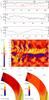Fig. 3 Energies of differential rotation (black solid lines) and mean toroidal magnetic field (red dashed) as functions of time from Runs G1, G2, and G3 (panels a)–c)). Panel d) shows the azimuthally averaged azimuthal magnetic field at r = 0.98 R⊙ from Run G2. The vertical dashed lines indicate the high and low states of differential rotation. Panels e) and f) show the time-averaged rotation profiles in Run G2 from the high and low states indicated as blue dotted and dashed lines in panel b).

Our results appear to stand apart from similar studies in full spherical shells (e.g., Nelson et al. 2013; Hotta et al. 2016) in that the differential rotation is strongly quenched as a function of the magnetic Reynolds number. However, in Nelson et al. (2013) the values of Rm′ (=2πRe_M) correspond to a range of 8...32 in Re_M in our units where the radial and latitudinal differential rotation decrease by about 30 per cent. This is roughly consistent with our results. On the other hand, Hotta et al. (2016) reached higher values of Re_M than in the present study, but no strong quenching was reported. The reason might be that their models are rotating substantially slower than ours, leading to weaker magnetic fields and a weaker back-reaction to the flow. Furthermore, in these models, the differential rotation is strongly influenced by their SGS heat flux, which transports one third of the luminosity. Another obvious candidate for explaining the difference is the wedge geometry used in the current simulations. However, we note that earlier simulations with a similar setup did not show a marked trend in the energy of the differential rotation as the azimuthal extent of the domain was varied (see Table 1 of Käpylä et al. 2013). However, results of Boussinesq simulations of convective dynamos have shown a similar change as a function of the magnetic Prandtl number (Schrinner et al. 2012). The drop in the amplitude of the differential rotation was associated with a change in the dynamo mode from an oscillatory multipolar solution to a quasi-steady dipolar configuration (cf. Fig. 15 of Schrinner et al. 2012) that prevents strong differential rotation from developing. We do not find a strong dipole component in our simulations (see Sect. 4.2.3). However, the strong suppression of the differential rotation often coincides with the appearance of a small-scale dynamo (see Table 1 and the discussion in the Sect. 4.1.2) or a change in the large-scale dynamo mode as discussed above.

4.1.2. Angular momentum transport

The azimuthally averaged z-component of the angular momentum is governed by the equation $\begin{array}{ccc}& & \frac{\mathit{\partial }}{\mathit{\partial t}}\mathrm{\left(}\mathit{\rho }{\mathit{\varpi }}^{\mathrm{2}}\mathrm{\Omega }\mathrm{\right)}\mathrm{+}\mathrm{\nabla }\mathrm{·}\mathrm{\left\{}\mathit{\varpi }\mathrm{\right[}\mathit{\varpi }\mathit{\rho U}\mathrm{\Omega }\mathrm{+}\mathit{\rho }{\mathit{u}}_{\mathit{\phi }}\mathit{u}\mathrm{-}\mathrm{2}\mathit{\nu \rho }\mathrm{S}\mathrm{·}\mathit{\phi ̂}\\ & & \end{array}$(27)where ϖ = rsinθ is the lever arm, and velocity and magnetic field have been decomposed into mean and fluctuating parts according to ${\mathit{U}}_{\mathit{i}}\mathrm{=}{\overline{\mathit{U}}}_{\mathit{i}}\mathrm{+}{\mathit{u}}_{\mathit{i}}$ and ${\mathit{B}}_{\mathit{i}}\mathrm{=}{\overline{\mathit{B}}}_{\mathit{i}}\mathrm{+}{\mathit{b}}_{\mathit{i}}$. We denote the Reynolds and Maxwell stresses as ${\mathrm{𝒬}}_{\mathit{ij}}\mathrm{=}\overline{{\mathit{u}}_{\mathit{i}}{\mathit{u}}_{\mathit{j}}}$ and ${\mathrm{ℳ}}_{\mathit{ij}}\mathrm{=}\mathrm{-}\overline{{\mathit{b}}_{\mathit{i}}{\mathit{b}}_{\mathit{j}}}\mathit{/}{\mathit{\mu }}_{\mathrm{0}}\overline{\mathit{\rho }}$, respectively. We note that Eq. (27) differs from the formulation of Brun et al. (2004), for instance, in that we have retained terms containing the mass flux ρU in the contributions corresponding to the meridional circulation. This is because in our fully compressible setup, ∇·ρU is non-zero. This is particularly important for the average radial mass flux $\overline{\mathit{\rho }{\mathit{U}}_{\mathit{r}}}$. However, it turns out that the effects of compressibility in the Reynolds stress and the viscous terms are negligible. This means that terms of the form $\overline{\mathrm{(}\mathit{\rho }{\mathit{u}}_{\mathit{i}}{\mathrm{)}}^{\mathrm{\prime }}{\mathit{u}}_{\mathit{j}}}$, where the prime denotes fluctuations, $\overline{\mathit{\rho }{\mathit{u}}_{\mathit{i}}{\mathit{u}}_{\mathit{j}}}$, and $\mathit{\nu }\overline{\mathit{\rho }{\mathit{u}}_{\mathit{i}\mathrm{;}\mathit{j}}}$, are neglected.

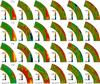Fig. 4 From left to right: Reynolds, Maxwell, and total stress components , ℳrφ, Trφ, , ℳθφ, and Tθφ for Runs C2 (top), C3, C4, and C5 (bottom). Data nearer than 2.5° from the latitudinal boundaries are not shown, so as to emphasize the structures at lower latitudes. The yellow contours denote the zero levels in each panel.

The main generator of differential rotation is commonly thought to be the Reynolds stress and in particular its non-diffusive contribution that is due to the Λ effect (Rüdiger 1980, 1989). Distinguishing the contributions from the Λ effect and the turbulent viscosity is currently only possible using assumptions regarding either of the two coefficients and computing the other from the Reynolds stress (e.g., Käpylä et al. 2014; Karak et al. 2015; Warnecke et al. 2016a). We do not attempt this here, but study the total turbulent stress and the anisotropy parameters realized in simulations with varying magnetic Reynolds number. Figure 4 shows the off-diagonal Reynolds stress components, and , from Runs C2 to C5 with Re_M varying between 14 and 146. The spatial structures of the two stress components remain relatively similar in Runs C2, C3, and C4. Neither of the stresses shows a monotonous behavior as functions of Re_M, both being generally smaller in Run C3 than in Runs C2 and C4. However, in Run C5 the overall magnitude is decreased by a factor of two for and about 15 per cent for . No corresponding decrease is observed in the diagonal components of the stress, whose overall magnitude is given by the fluid Reynolds number; see Table 1.

We find that for magnetic Reynolds numbers up to roughly 30, the off-diagonal Maxwell stresses are smaller than the corresponding Reynolds stresses. The magnitude of the vertical component ℳ_rφ is between a quarter and a half of , whereas for the horizontal component the difference is greater. With higher Re_M, the Maxwell stresses attain similar profiles as the Reynolds stresses but with opposite signs. The magnitudes of the Maxwell stresses increase with Re_M such that they become comparable to and locally even larger than the Reynolds stresses at the highest magnetic Reynolds numbers. The total vertical stress T_rφ decreases for Runs C2–C4 such that the effect is most clear near the equator. For Run C5 the vertical stress is dominated by the Maxwell stress near the equator. The horizontal component T_θφ decreases monotonically as Re_M increases. The near cancellation of the total stress at high Re_M is likely to contribute significantly to the quenching of differential rotation. These results are apparently at odds with those of Karak et al. (2015), who reported that the Maxwell stress is an order of magnitude smaller than the Reynolds stress. However, their simulations were in a regime near the transition between anti-solar and solar-like rotation profiles with relatively weak and intermittent large-scale dynamos.

In Set F with anti-solar differential rotation the Reynolds stresses show only a weak decreasing trend as a function of Re_M with a corresponding increase in the Maxwell stress (not shown). The vertical Maxwell stress has an opposite sign in comparison to the Reynolds stress in all cases, while a similar tendency for the horizontal stress is not so clear. The magnitude of the vertical Maxwell stress is roughly half of the corresponding Reynolds stress, while the amplitude of the horizontal Maxwell stress is significantly weaker than the horizontal Reynolds stress. The much weaker quenching of the total turbulent stress in Set F is consistent with a clearly milder decrease of the differential rotation than in the other sets.

Assuming that the turbulent viscosity follows a naive mixing length estimate, the quenching of the differential rotation can indicate that the Λ effect is more severely quenched by the large-scale magnetic field at high magnetic Reynolds numbers. Another possibility is that small-scale magnetic fields generated by an efficient small-scale dynamo contribute to enhancing the turbulent viscosity. In a recent paper, Hotta et al. (2016) suggested that the small-scale dynamo at high Re_M suppresses velocity at small scales and facilitates the growth of the large-scale magnetic fields. First-order smoothing estimates for isotropic and homogeneous turbulence (M. Rheinhardt, private communication) suggest that turbulent viscosity acquires a contribution ${\mathit{\nu }}_{\mathrm{t}}^{\mathrm{\left(}\mathrm{SSD}\mathrm{\right)}}\mathrm{=}\frac{\mathrm{1}}{\mathrm{3}}{\mathit{b}}_{\mathrm{rms}}^{\mathrm{\left(}\mathrm{0}\mathrm{\right)}}{\mathit{k}}_{\mathrm{f}}^{-1}$, where ${\mathit{b}}_{\mathrm{rms}}^{\mathrm{\left(}\mathrm{0}\mathrm{\right)}}$ is the rms-value of the saturated fluctuating magnetic field due to small-scale dynamo. We find that the fluctuating magnetic field energy grows monotonically as a function of Re_M; see Table 2. A corresponding increase of turbulent viscosity would be compatible with a strong decrease of differential rotation. However, we find two counter-examples: in Set A, no SSD is present but the differential rotation still experiences strong quenching, and in Set F, an SSD is present but differential rotation remains strong. Furthermore, the dependence of the Λ effect on small-scale magnetic fields is currently unknown. Thus the question of the effect of small-scale dynamo on the turbulent transport of angular momentum at large scales remains open.

Fig. 5 Anisotropy parameters AV (left) and AH (right) for the same runs as in Fig. 4. The yellow contours denote the zero levels in each panel.

We also show the anisotropy parameters (Fig. 5) $\begin{array}{ccc}{\mathit{A}}_{\mathrm{V}}& \mathrm{=}& \frac{{\mathrm{𝒬}}_{\mathit{\phi \phi }}\mathrm{-}{\mathrm{𝒬}}_{\mathit{rr}}}{{\mathrm{𝒬}}_{\mathit{\phi \phi }}\mathrm{+}{\mathrm{𝒬}}_{\mathit{rr}}}\mathit{,}\\ {\mathit{A}}_{\mathrm{H}}& \mathrm{=}& \frac{{\mathrm{𝒬}}_{\mathit{\phi \phi }}\mathrm{-}{\mathrm{𝒬}}_{\mathit{\theta \theta }}}{{\mathrm{𝒬}}_{\mathit{\phi \phi }}\mathrm{+}{\mathrm{𝒬}}_{\mathit{\theta \theta }}}\mathit{,}\end{array}$which are proportional to the vertical and horizontal Λ effects in mean-field hydrodynamics (Rüdiger 1980) under the assumption of slow rotation (see also the numerical results of Käpylä & Brandenburg 2008). Again the differences between Runs C2 and C3 are relatively small, whereas in Runs C4 and C5 the mostly positive A_V at mid-latitudes in lower-Re_M runs gives way to negative values. According to mean-field theory, this corresponds to a sign change of the vertical Λ effect that is responsible for generating radial differential rotation (Rüdiger 1980). The magnitude and the spatial distribution of the horizontal anisotropy parameter A_H are significantly different in Run C5 in comparison to the other runs, whereas the differences between the other runs are less significant. The negative values of A_H at mid-latitudes in Runs C2–C4 coincide with the minimum in the angular velocity, suggesting that the horizontal Λ effect is negative there. In Run C5 the overall magnitude of A_H is diminished near the surface at low latitudes. Along with the change of sign of A_V, this is likely to contribute to the reduced differential rotation as a function of Re_M. However, more theoretical work is needed to distinguish the effects of the small- and large-scale magnetic fields on the angular momentum transport.

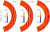Fig. 6 Radial (divFr, left panel) and latitudinal (divFθ, middle) parts of the divergence of the angular momentum fluxes. The right panel shows the total divergence. The units are given in the legend. Data taken from Run C3.

The discussion above is valid when the angular momentum is in a statistically steady state demanding that the sum of two terms, divF_r + divF_θ, vanishes, that is, $\begin{array}{ccc}\frac{\mathrm{1}}{{\mathit{r}}^{\mathrm{2}}}\frac{\mathit{\partial }\mathrm{\left(}{\mathit{r}}^{\mathrm{2}}{\mathrm{ℱ}}_{\mathit{r}}\mathrm{\right)}}{\mathit{\partial r}}\mathrm{+}\frac{\mathrm{1}}{\mathit{r}\sin \mathit{\theta }}\frac{\mathit{\partial }\mathrm{\left(}\sin \mathit{\theta }{\mathrm{ℱ}}_{\mathit{\theta }}\mathrm{\right)}}{\mathit{\partial \theta }}\mathrm{\equiv }\mathrm{div}{\mathit{F}}_{\mathit{r}}\mathrm{+}\mathrm{div}{\mathit{F}}_{\mathit{\theta }}\mathrm{=}\mathrm{0}\mathit{,}& & \end{array}$(30)where ${\mathrm{ℱ}}_{\mathit{r}}\mathrm{=}\mathit{\varpi }[\mathit{\varpi }\overline{\mathit{\rho }{\mathit{U}}_{\mathit{r}}}\mathrm{\Omega }\mathrm{+}\overline{\mathit{\rho }}{\mathrm{𝒬}}_{\mathit{r\phi }}\mathrm{-}\mathit{\nu \rho \varpi }\frac{\mathit{\partial }\mathrm{\Omega }}{\mathit{\partial r}}\mathrm{-}{\mathit{\mu }}_{\mathrm{0}}^{-1}\mathrm{(}{\overline{\mathit{B}}}_{\mathit{\phi }}{\overline{\mathit{B}}}_{\mathit{r}}\mathrm{+}\overline{{\mathit{b}}_{\mathit{r}}{\mathit{b}}_{\mathit{\phi }}}\mathrm{)}]\mathit{,}$(31)and ${\mathrm{ℱ}}_{\mathit{\theta }}\mathrm{=}\mathit{\varpi }[\mathit{\varpi }\overline{\mathit{\rho }{\mathit{U}}_{\mathit{\theta }}}\mathrm{\Omega }\mathrm{+}\overline{\mathit{\rho }}{\mathrm{𝒬}}_{\mathit{\theta \phi }}\mathrm{-}\mathit{\nu \rho }\frac{\mathit{\varpi }}{\mathit{r}}\frac{\mathit{\partial }\mathrm{\Omega }}{\mathit{\partial \theta }}\mathrm{-}{\mathit{\mu }}_{\mathrm{0}}^{-1}\mathrm{(}{\overline{\mathit{B}}}_{\mathit{\phi }}{\overline{\mathit{B}}}_{\mathit{\theta }}\mathrm{+}\overline{{\mathit{b}}_{\mathit{\theta }}{\mathit{b}}_{\mathit{\phi }}}\mathrm{)}]\mathit{.}$(32)Figure 6 shows representative results from Run C3 for the terms divF_r and divF_θ, as well as their sum. We find that the radial and latitudinal contributions have similar structures but opposite signs and that their sum is at most roughly eight per cent of the individual components. The elongated structures at low latitudes within the tangent cylinder are due to the meridional circulation that yields the dominant contribution to the divergence. We note that neither the radial nor the latitudinal fluxes need to individually cancel for the divergence to vanish.

4.2. Large-scale magnetic fields and dynamo cycles

4.2.1. General considerations

We find no dynamos in the lowest magnetic Reynolds number cases Runs A1, A2, B1, C1, and D1, which are in the range Re_M = 5...9. On the other hand, the highest magnetic Reynolds numbers clearly exceed critical values for small-scale dynamo action to occur in simpler setups (e.g., Schekochihin et al. 2005). In the present simulations the small- and large-scale dynamos can be excited at the same time, and separating the two is not directly possible. We therefore resort to runs where we artificially suppress the large-scale (φ-averaged) magnetic fields at each time step. This eliminates the large-scale dynamo and growing magnetic fields can be associated with a small-scale dynamo. We have performed such runs for each of the cases where a dynamo is observed and find that a small-scale dynamo is excited in Runs B5, C5, D4, D5, E3, E4, F4, G2, and G3.

4.2.2. Cycle detection using D² analysis

Using the D² statistic discussed in Sect. 3, we separately analyzed radial and azimuthal components of the mean magnetic field. In the former case we included all the data near the polar region (55° ≤ | 90°−θ | ≤ 75°) and in the latter case data around mid-latitude region (10° ≤ | 90°−θ | ≤ 45°). We considered data above 0.94 R_⊙ and analyzed the northern and southern hemispheres separately.

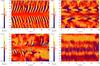Fig. 7 Azimuthally averaged azimuthal magnetic field near the surface from Runs B2 (top left), D3 (top right), B3 (bottom left), and F3 (bottom right) with poleward (PW), equatorward (EW), irregular (IR), and quasi-stationary (QS) dynamo solutions, respectively.

The results of the analysis are listed in Table 3. We required that at least five full cycles were covered for each trial period in the period search range. To meet this criterion, we adjusted the upper limit of the period search range according to the length of the dataset, while the lower limit was always fixed at one year. We set the lower limit for the coherence length range to two cycles per given period and the upper value was determined by the dataset length. However, in some cases the longest possible trial period was still shorter than two years, in which cases the analysis was deemed infeasible. This situation was encountered for Run G3, which has therefore not been included in Table 3. Furthermore, Runs A1, A2, B1, C1, and D1 without dynamos were not analyzed.

All the cycle lengths given in Table 3 are significant with the p-values lower than 1%. More precisely, in our case the p-value represents a probability that a cycle with a given period would appear by chance out of white-noise data with the same distribution as the original data. In those cases where the obtained D² spectrum contained no significant minima, no cycle was detected. However, here we must also note that as a result of narrowing the period search range in some cases, it is possible that the real cycle length is located outside the range and we did not detect it. This is particularly relevant for the runs at high magnetic Reynolds numbers where the time series are short.

In all the sets, especially when the highest Reynolds number cases are excluded, the cycle lengths are found to increase as functions of the magnetic Prandtl number. This shows that the dynamo period is sensitive to the strength of the magnetic diffusion such that when the diffusion is decreased, and correspondingly the diffusion timescale increases, the dynamo period increases.

4.2.3. Dynamo modes

Given that recent simulations reproduce solar-like magnetic cycles with equatorward migration (hereafter EW) of activity belts, it is of interest to probe the parameter space to determine when such solutions are excited. After identifying cyclic solutions with the D² statistics, we classified them as EW or PW (poleward) based on the migration direction of the dynamo wave at low latitudes between ± 10° and ± 45°. We also find quasi-stationary (hereafter QS) solutions in Set F. When a clear classification by visual inspection could not be made, we classify the solution as irregular (IR). In some cases features from more than one class can be present, for instance, an equatorward cyclic variation in addition to a quasi-stationary background. This solution is classified as EW/QS, but typically such cases are quite uncertain and are indicated by brackets in the last column of Table 3. No large-scale dynamo action is denoted by ND. In Fig. 7 we show time-latitude plots of the azimuthally averaged azimuthal magnetic field ${\overline{\mathit{B}}}_{\mathit{\phi }}$ from four runs exemplifying each of the main dynamo modes discussed above.

We first consider the Sets A–D with Ω₀ = 5Ω_⊙. For Pr_SGS = 0.25 (Set A) and moderate Re_M we obtain solutions with clear poleward migration. This type of dynamos was first obtained in the pioneering studies of Gilman (1983) and Glatzmaier (1985). Solutions showing poleward migration have been reported more recently by many groups (e.g., Käpylä et al. 2010b; Brown et al. 2011; Schrinner et al. 2012). In one case (Run A3) we see a hemispheric dynamo with poleward migration, similar to those reported by Busse (2002) and Gastine et al. (2012), for example. In the largest Re_M case (Run A5) the clear oscillatory solutions of the runs with smaller Reynolds numbers give way to possibly irregularly reversing or quasi-stationary large-scale fields. The time series is too short, however, for possible cycles to be detected. For Pr_SGS = 0.5 (Set B) we find a PW mode excited in the case Re_M = 12 (Run B2). At intermediate Re_M (Runs B3 and B4) the solutions mostly show irregularly reversing fields, although features from both PW and EW modes can be discerned at times; see the lower left panel of Fig. 7. The highest Reynolds number case (Run B5) appears to return to a poleward oscillatory mode with a longer cycle period. However, the large-scale field shows only four reversals in the 24-yr duration of the simulation and the D² statistic captures this only in one of the four analyzed cases. Therefore the classification of this run as PW is deemed less reliable than those of the other runs in this set.

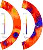Fig. 8 Azimuthally averaged azimuthal magnetic field ${\overline{\mathit{B}}}_{\mathit{\phi }}$ (color contours) in units of kG and the fields lines of the poloidal field (continuous and broken lines for clockwise and anticlockwise loops, respectively). Left: data from Run B2 averaged over three months near a cycle maximum at t = 70 yr. Right: data from Run A5 averaged over the last ten years of the run.

For Pr_SGS ≥ 1 (Sets C and D) we often find solutions with EW migration (Runs C2, C3, D2, D3, and D4). In Run D4 the solution is clearly EW, but the time series covers only three full cycles and is therefore not detected by D². The transition from poleward migrating to equatorward migrating solutions at intermediate magnetic Reynolds numbers coincides with the change of the rotation profile from runs with consistently positive radial gradient of Ω to ones with a minimum of Ω at mid-latitudes where ∂Ω /∂r< 0 as Pr_SGS increases. The change in the dynamo mode fits with the interpretation in terms of a classical dynamo wave obeying the Parker-Yoshimura rule (Warnecke et al. 2014, 2016b). For the highest magnetic Reynolds number cases in Sets C and D we again observe possibly quasi-stationary or irregular configurations. This classification is based on significantly shorter time series than in the other cases, and it is possible that there are cycles that are much longer than in the low-Re_M cases or that a prolonged transient is still in progress. These results appear to be in agreement with those of Schrinner et al. (2012), who found a transition from oscillatory dynamos to non-oscillatory ones at a roughly comparable Re_M for Boussinesq convection in spherical shells. They also showed that in the high-Pr_M regime the two bistable branches of dynamo solutions merge and that only strongly dipolar dynamos with weak differential rotation survive. However, Gastine et al. (2012) have shown that for sufficiently density stratified cases the dipolar branch does not exist at least for moderate values of Re_M. Our simulations with moderate density stratification of H_ρ ≈ 3, where H_ρ = −(∂lnρ/∂r)^-1 is the density scale height, do not indicate that a dipolar mode takes over at high Re_M, see Fig. 8 for a representative result from Run A5. This is consistent with the results of Gastine et al. (2012), who found no dipole-dominated dynamos for H_ρ ≳ 2.

The realized solutions from the runs in Sets A–D are plotted in the (Pr_SGS,Pr_M)-plane in Fig. 9. We find that the low and intermediate Re_M runs produce cyclic solutions with PW for low Pr_SGS and EW for high Pr_SGS. The case Pr_SGS = 0.5 works as a watershed between the two cyclic regimes. The dynamos at high Re_M are fundamentally different from their more diffusive counterparts in that the differential rotation is almost absent. Although the ratio of the energies in the mean poloidal to toroidal components is not significantly different in the high-Re_M runs in comparison to lower-Re_M runs in each set, the dynamos at the high-Re_M regime can be of α² type. Substantiating this claim, however, requires that the turbulent transport coefficients relevant for the maintenance of large-scale magnetic fields are extracted from the simulations and applied in corresponding mean-field models, which is not within the scope of the present study.

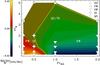Fig. 9 Color contours: radial derivative of Ω at r = 0.85 R⊙ averaged from latitudes + 25° and −25°. The dynamo modes realized in Sets A–D are overplotted with abbreviations ND, PW, EW, IR, and QS. The thick yellow curve indicates the zero level of ∂Ω /∂r. Overlapping symbols denote solutions that show characteristics from several modes, while question marks indicate that the classification is uncertain because of the insufficient length of the data set.

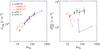Fig. 10 Energy densities of the total magnetic field (left panel), and the azimuthally averaged fields (right) from Sets C (black dashed line) and G (black solid), from two sets of runs by Nelson et al. (2013; solid and dashed red lines) and from Hotta et al. (2016; blue solid lines). The red solid line consists of data from cases D3, D3a, and D3b of Nelson et al. (2013) with PrM = const. = 0.5. Correspondingly, the dashed red line shows data from cases D3, D3-pm1, and D3-pm2 of Nelson et al. (2013) with PrM varying from 0.5 to 2. From Hotta et al. (2016) we show data for cases “Low”, “Medium”, and “High”.

In Set E we find a PW solution for the lowest Re_M (Run E1), whereas at higher Re_M we find IR (E2) and irregular/quasi-stationary (E3 and E4) configurations. Generally, Set E behaves similarly as Sets A–C, that is, a transition from oscillatory dynamos at intermediate Re_M to quasi-stationary or irregularly varying solutions at high Re_M. However, Run B1 of Warnecke et al. (2016a) is similar to Run E2, but with Pr_SGS = 2 instead of 1 shows EW. Set F is qualitatively different from the other sets similarly as for the differential rotation. The large-scale magnetic fields show a quasi-stationary configuration in all of the runs in Set F. In Run G2 the modulation of the differential rotation was shown to be related to a changing large-scale dynamo mode that is either EW or QS; see panels b and d of Fig. 3. In the highest-Re_M case, Run G3, the two competing modes appear to be present again, but the short data set length renders such classifications preliminary at best.

4.2.4. Saturation level of large-scale magnetic fields

For the total magnetic energy we find a monotonically increasing trend as a function of Re_M in all sets, see representative results in the left panel of Fig. 10 and Table 2. The absolute value of the axisymmetric parts of the poloidal and toroidal magnetic fields shows monotonically decreasing trends only in Set F with anti-solar differential rotation. In the other sets the energies of the poloidal and toroidal mean fields typically do not behave monotonically as functions of Re_M. However, given the large temporal variations, our results are compatible with mean magnetic field energies converging to constant values at high magnetic Reynolds numbers, see the right panel of Fig. 10 for the results of Sets C and G. The same conclusion also applies to Set F. The findings for the mean magnetic fields appear to contradict the results of Nelson et al. (2013), who found a monotonically decreasing trend as a function of Re_M; see Fig. 10.

The main difference to the simulations of Nelson et al. (2013) is that their models were done with a full spherical shell as opposed to the wedge geometry used here, and that magnetic field boundary condition at the outer radial boundary uses extrapolation to a potential field rather than a radial field condition as in the present study. Furthermore, Nelson et al. (2013) considered anelastic models, whereas in our case the gas is fully compressible. Simulations with forced turbulence in spherical shells with coronal envelopes have shown that a higher field strength can be achieved when the magnetic field at the boundary is not restricted to being purely radial (Warnecke & Brandenburg 2014). Furthermore, Nelson et al. (2013) used profiles for ν and η, which are absent in our study. The constant diffusion coefficients used here may lead to a steeper increase of the magnetic field energy than in the runs of Nelson et al. (2013), where the local value of Re_M is significantly higher in the deeper layers. Detailed comparisons of diffusion schemes and parameter values are presented in Tables A.1 and A.2.

It is difficult to assess which of these differences is the most important. However, a plausible candidate is the change in topology of the field in the full-sphere simulations of Nelson et al. (2013). As described in Käpylä et al. (2013), the large-scale magnetic field can become dominated by low-order non-axisymmetric modes, and therefore applying an axisymmetric mean will average out such field contributions (see their Fig. 16 and Table 2). Evidence of such non-axisymmetric modes can be seen in the instantaneous magnetic fields in Figs. 4 and 6 of Nelson et al. (2013). However, it is not possible to assess how the degree of non-axisymmetry behaves as a function of Re_M in the results of Nelson et al. (2013), and a direct comparison is therefore not possible.

In another recent study, Hotta et al. (2016) presented results from less rapidly rotating (Ω = Ω_⊙) simulations at high values of Re_M. Such simulations are less likely to contain significant non-axisymmetric modes. Their main claim is that whereas the mean magnetic energy decreases at intermediate Re_M, it recovers as Re_M is increased further. We have included their results in Fig. 10 for comparison. However, only a rough comparison is possible as only three data points are available and a jump occurs between the two lowest-Re_M runs, which is caused by a switch from explicit diffusion to a numerical slope-limited scheme. The absolute values for the mean fields are also lower than ours, probably because their large-scale dynamo is less efficient than in the present study because of their slower rotation. Only the trend as a function of Re_M can therefore be compared with the current results or with those of Nelson et al. (2013). The results of Hotta et al. (2016) are more in line with ours, but the degree of temporal variations is indicated only in passing. Hotta et al. (2016) stated that during the last 200 days the mean magnetic field energy in the simulation high is almost 2.5 times higher than in the time average over the full duration (50 yr) of the simulation. It is not possible to accurately assess the steepness of the increasing trend of the energy of the mean field as a function of Re_M.

5. Conclusions

We find that, as the SGS Prandtl number (responsible for SGS turbulent transport) is increased, the rotation profiles realized in the simulations develop a region of negative shear at mid-latitudes. At moderate Re_M this latitude coincides with a transition from poleward-migrating to equatorward-migrating dynamo modes. This can be explained by interpreting the solutions as dynamo waves propagating along the isocontours of constant shear (Parker 1955; Yoshimura 1975). However, it appears that, as Pr_M is sufficiently high (corresponding to high Re_M), the regular cycles give way to quasi-stationary or irregularly varying solutions. However, as a result of computational constraints, the time series of these runs are typically significantly shorter than of the lower-Re_M runs, so that cyclic solutions with long cycle periods cannot be ruled out.

We also find that the cycle length of the dynamo solution undergoes a systematic increase when the magnetic Prandtl number is increased: seemingly independent of the other parameters, the decreasing magnetic diffusivity leads to longer cycles. The highest Reynolds number runs are, however, too short for our period analysis to work conclusively.

We find a strong dependence of the differential rotation on the magnetic Reynolds number so that for the highest values of Re_M both radial and latitudinal shear are almost absent. The strongest quenching tends to appear in cases where a small-scale dynamo is present. However, there are exceptions. The physical reason for the quenching is therefore unclear, but several mechanisms appear plausible. First, the small-scale magnetic field can enhance turbulent viscosity or quench the Λ-effect responsible for maintaining differential rotation. Suppression of small-scale flows that are due to the small-scale magnetic fields has been suggested by Hotta et al. (2016). We find that at intermediate Re_M, the Maxwell stress is on the same order of magnitude as the Reynolds stress and becomes comparable at high Re_M. Because of their opposite signs, the total stress is diminished. We expect that for intermediate and in particular for high Re_M, the Maxwell stress plays an important role in the angular momentum transport. Second, the dependence of turbulent transport on the large-scale magnetic field is Re_M-dependent and can lead to enhanced quenching in the parameter regime studied here in comparison to earlier more laminar simulations. However, for a limited parameter range we find that the system vacillates between two states where either the differential rotation is strong and mean magnetic field relatively weak, or vice versa. Furthermore, the temporal variations appear to increase as the Rayleigh and Reynolds numbers are increased. Finally, we find that in cases where the differential rotation is anti-solar, the quenching is much less prominent, possibly due to significantly weaker mean fields generated in those cases.

The total magnetic energy grows monotonically as a function of Re_M in all of our runs. The energy of the azimuthally averaged fields is in all cases consistent with increasing or constant mean fields at high Re_M. This is apparently at odds with the anelastic full-sphere simulations of Nelson et al. (2013), who found a steeply declining trend with magnetic Reynolds number. However, their relatively rapidly rotating (Ω = 3Ω_⊙) simulations also allow significant low-order non-axisymmetric modes to develop that will not show up in azimuthal averaging. A fair comparison is therefore not possible without a proper assessment of the non-axisymmetric contributions. Our results are more in line with those of Hotta et al. (2016), who used a model rotating at the solar rate where the large-scale fields are more clearly axisymmetric.

A possible source of discrepancies between the current and previous studies is the use of wedge geometry. Rigorous comparisons between wedges and fully spherical simulations have not been done so far. However, runs with similar parameters (Rayleigh, Taylor, and Prandtl numbers) produce results that are in qualitative agreement; compare the results of Käpylä et al. (2010b) regarding cyclic dynamos with those of Brown et al. (2011), for instance. Similarly, the more recent simulations showing equatorward migration (Käpylä et al. 2012; Augustson et al. 2015) appear to support the validity of the wedge approach. Furthermore, wedges with full 2π extent in longitude produce dynamos dominated by non-axisymmetric large-scale fields with azimuthal dynamo waves (Käpylä et al. 2013; Cole et al. 2014) that are also routinely seen in anelastic full-sphere simulations (e.g., Yadav et al. 2015). Last, the transition from anti-solar to solar-like differential rotation occurs at very similar Coriolis numbers in a wide range of simulations, including wedges with artificially increased luminosity and rotation rate (Gastine et al. 2014). The various modeling approaches also use a range of different SGS models and parameter values (see Tables A.1 and A.2) and are still able to reproduce similar large-scale phenomena. These comparisons suggest that the current results obtained in wedges are likely to be realized in fully spherical simulations in the same parameter regime.

Our final conclusion is that the current simulations are not near an asymptotic regime where the large-scale results would be independent of the microphysical diffusion coefficients. This is most strikingly demonstrated by the steep quenching of the differential rotation and the disappearance of regularly oscillating large-scale magnetic fields at high values of Re_M.

Acknowledgments

The authors thank an anonymous referee for useful comments and Paul Charbonneau and Hideyuki Hotta for providing information regarding their models. The simulations were performed using the supercomputers hosted by CSC – IT Center for Science Ltd. in Espoo, Finland, who are administered by the Finnish Ministry of Education and in the HLRS supercomputing center in Stuttgart, Germany through the PRACE allocation “SOLDYN”. Financial support from the Academy of Finland grants No. 136189, 140970, 272786 (P.J.K.), and 272157 to the ReSoLVE Centre of Excellence (P.J.K., M.J.K.), as well as the Swedish Research Council grants 621-2011-5076 and 2012-5797, and the Research Council of Norway under the FRINATEK grant 231444 are acknowledged. J.W. acknowledges funding by the Max-Planck/Princeton Center for Plasma Physics and funding from the People Programme (Marie Curie Actions) of the European Union’s Seventh Framework Programme (FP7/2007-2013) under REA grant agreement No. 623609.

References

Appendix A: Comparison to other simulation methods

The purpose of this appendix is to compare the diffusion schemes and estimates of the Prandtl numbers in the present study with several methods presented in the literature. We consider the papers by Nelson et al. (2013) and Hotta et al. (2016) that are discussed in the main text as well as the study of Ghizaru et al. (2010), which represents another established simulation method; see Tables A.1 and A.2 for details.

Estimating the Prandtl number from simulations using the solar luminosity requires that the value of the radiative diffusivity in the solar convection zone is known. For the following we use an estimate of this quantity at r = 0.85 R_⊙. Standard solar models (e.g., Stix 2002) indicate that radiation carries roughly ten per cent of the flux at this radius, such that L^rad ≈ 0.1 L_⊙. Using Eq. (6), we can write ${\mathit{L}}^{\mathrm{rad}}\mathrm{=}\mathrm{4}\mathit{\pi }{\mathit{r}}^{\mathrm{2}}{\mathit{F}}^{\mathrm{rad}}\mathrm{=}\mathrm{-}\mathrm{4}\mathit{\pi }{\mathit{r}}^{\mathrm{2}}\mathit{K}{\mathit{\partial }}_{\mathit{r}}\mathit{T}\mathit{.}$(A.1)We then use the definition of the heat conductivity K = c_Pρχ, assume that the temperature gradient is close to the adiabatic one, ∂_rT ≈ −g/c_P, and insert g = GM_⊙/r² to obtain 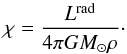$\mathit{\chi }\mathrm{=}\frac{{\mathit{L}}^{\mathrm{rad}}}{\mathrm{4}\mathit{\pi G}{\mathit{M}}_{\mathrm{\odot }}\mathit{\rho }}\mathrm{·}$(A.2)Using the values quoted above and ρ ≈ 50 kg m^-3 (Stix 2002), we find that χ ≈ 5 × 10² m² s^-1 for the Sun at r = 0.85 R_⊙.

The solar luminosity is adopted in the study of Nelson et al. (2013), yielding a radiative diffusion coefficient on the order of the estimate from Eq. (A.2). The authors did not present a detailed description of their model, however, but referred to Brown et al. (2010), where the corresponding quantity is denoted as κ_r. Furthermore, the values of ν at mid-convection zone depth are in the range 6...13 × 10⁷ m² s^-1 for their cases D3[a, b, pm1, pm2], and a value of 2 × 10⁶ m² s^-1 is estimated for case S3 with a Smagorinsky SGS model. These yield Prandtl numbers on the order of 10⁵ and 10⁴, respectively. For the model “Low” of Hotta et al. (2016), only the surface value ν = 10⁸ m² s^-1 is given. As ν is proportional to ρ^{− 1 / 2}, the value at mid-convection zone depth is a few times 10⁷ m² s^-1 and the Prandtl number is of the order of 10⁵. For their cases “Medium”, “High”, and “High-S”, a slope-limited diffusion scheme is used, so that estimating the diffusion coefficients is non-trivial. However, they computed the Reynolds number (hereafter Re_SL) based on the Taylor microscale that was obtained from kinetic energy spectra. They found that the Reynolds numbers for “High” and “High-S” are roughly an order of magnitude larger than for “Low”, whereas for “Low” and “Medium” they are comparable. Assuming that the turbulent velocities in all cases are of similar strengths, we can estimate “slope-limited diffusion viscosities” from ν_SL = ν_LowRe_Low/ Re_SL. We therefore infer that the value of the Prandtl number in the model “Medium” is 10⁵ and an order of magnitude smaller in the models “High” and “High-S”. In these runs, the surface value of the turbulent heat conductivity is κ = 2 × 10⁹ m² s^-1 (H. Hotta, private communication), yielding Pr_SGS in the range 0.05...2 × 10^-3 for the runs of Hotta et al. (2016).

In principle, even a third Prandtl number can be defined based on the diffusion coefficient applied only to the mean (spherically symmetric) entropy profile. In the present study and also in that of Hotta et al. (2016), this coincides with the coefficient relevant for diffusing entropy fluctuations. However, the coefficients can also be different, which is the formulation often used in simulations performed with the anelastic spherical harmonic (ASH) code including those presented in Nelson et al. (2013). However, the value of the coefficient for mean entropy diffusion (κ₀) is not provided in the reference with a more detailed model description (Brown et al. 2010).

The Eulerian-Lagrangian (EULAG) code of Smolarkiewicz & Charbonneau (2013) employed by Ghizaru et al. (2010) uses quite a different approach and replaces radiative conduction by Newtonian cooling toward a prescribed thermodynamic state. The timescale of the cooling τ_c is typically on the order of 20 months (P. Charbonneau, private communication; see also Strugarek et al. 2016). This timescale would correspond to a radiative/SGS diffusion coefficient of χ = Δr²/τ_c ≈ 6 × 10⁸ m² s^-1, where Δr = 0.25 R_⊙. Although this comparison yields some insight about the entropy evolution, the cooling and diffusion processes cannot be directly equated. Therefore the concept of a Prandtl number does not appear suitable in that case. The diffusion of velocity, magnetic fields, and entropy fluctuations is due to the numerical scheme making the estimates of the other Prandtl numbers also problematic. Presumably the diffusivities of all variables at a given resolution are roughly similar such that Pr_SGS and Pr_M are on the order of unity. Hydrodynamic EULAG models with an otherwise similar setup to that of Ghizaru et al. (2010) yield estimates of viscosity and entropy diffusion in ranges ν_eff = 0.6...1.2 × 10⁸ m² s^-1 and κ_eff = 1...8 × 10⁷ m² s^-1, with Pr_SGS = ν_eff/κ_eff ≈ 1...8 (Strugarek et al. 2016).

We show the conversion factors for the definitions used in the current study for Péclet, fluid and magnetic Reynolds, and Coriolis numbers in Table A.2. The conversion for the results of Nelson et al. (2013) is straightforward, except that for the Coriolis number we have used the relation Ta = Co^′2Re^′2 to compute Co′ = 2πCo. The definition of the Rossby number in Nelson et al. (2013), Ro = ω/ 2Ω, is based on the vorticity ω = ∇ × u and corresponds to Co = Ro^-1k_ω/k_f, where k_ω = ω_rms/u_rms. The values of Co for the models of Nelson et al. (2013) correspond well to our simulations with Ω = 3Ω_⊙, see Table 1. In the case of the EULAG simulations we use the values quoted by Passos & Charbonneau (2014) for the Reynolds numbers (30...60 in their notation) divided by 2π and the estimate of Pr_SGS quoted above to compute Pe. The estimate of the Coriolis number is based on simulation data provided by P. Charbonneau. Finally, for the study of Hotta et al. (2016), the conversion of the fluid and magnetic Reynolds numbers is based on values given in the paper, whereas the estimates of Pe and Co are based on simulation data provided by H. Hotta. The values of Co are again in excellent agreement with our corresponding simulations with Ω = Ω_⊙; see Table 1.

We note that the simulations of Nelson et al. (2013) and Hotta et al. (2016) operate in a low-Pr_SGS regime that is also realized in the Sun, although in a much more extreme fashion. Such a regime is required especially in simulations with solar luminosity and rotation rate to lower the convective velocities and to achieve solar-like differential rotation (Käpylä et al. 2014; Hotta et al. 2016). However, the tradeoff is that the Péclet numbers are low and the evolution of entropy is significantly influenced by the SGS diffusion. It is not clear whether such an approach is more realistic than having Pr_SGS and Pr_M on the order of unity and Re, Re_M, and Pe≫ 1. We also note that the run times of the highest resolution runs are short: four years for “S3” in Nelson et al. (2013) and 500 days for “High-S” in Hotta et al. (2016), whereas transients and/or secular evolution in the high-Re_M regime can have a significantly longer timescale; see Figs 3b–d.

All Tables

All Figures

	Fig. 1 Top row: temporally averaged rotation profiles from Runs A3, B3, C3, and D3 with PrM = 1 and PrSGS varying from 0.25 (left) to 2 (right). Lower row: same as above, but for Runs C2, C3, C4, and C5 with PrSGS = 1 and PrM varying from 0.5 (left) to 5 (right).
In the text

	Fig. 2 Estimates of radial and latitudinal differential rotation ${\mathrm{\Delta }}_{\mathrm{\Omega }}^{\mathrm{\left(}\mathit{r}\mathrm{\right)}}$ and ${\mathrm{\Delta }}_{\mathrm{\Omega }}^{\mathrm{\left(}\mathit{\theta }\mathrm{\right)}}$, respectively, according to Eq. (26) for Sets A–F as indicated by the legend.
In the text

Fig. 3 Energies of differential rotation (black solid lines) and mean toroidal magnetic field (red dashed) as functions of time from Runs G1, G2, and G3 (panels a)–c)). Panel d) shows the azimuthally averaged azimuthal magnetic field at r = 0.98 R⊙ from Run G2. The vertical dashed lines indicate the high and low states of differential rotation. Panels e) and f) show the time-averaged rotation profiles in Run G2 from the high and low states indicated as blue dotted and dashed lines in panel b).

In the text

	Fig. 4 From left to right: Reynolds, Maxwell, and total stress components , ℳrφ, Trφ, , ℳθφ, and Tθφ for Runs C2 (top), C3, C4, and C5 (bottom). Data nearer than 2.5° from the latitudinal boundaries are not shown, so as to emphasize the structures at lower latitudes. The yellow contours denote the zero levels in each panel.
In the text

	Fig. 5 Anisotropy parameters AV (left) and AH (right) for the same runs as in Fig. 4. The yellow contours denote the zero levels in each panel.
In the text

	Fig. 6 Radial (divFr, left panel) and latitudinal (divFθ, middle) parts of the divergence of the angular momentum fluxes. The right panel shows the total divergence. The units are given in the legend. Data taken from Run C3.
In the text

	Fig. 7 Azimuthally averaged azimuthal magnetic field near the surface from Runs B2 (top left), D3 (top right), B3 (bottom left), and F3 (bottom right) with poleward (PW), equatorward (EW), irregular (IR), and quasi-stationary (QS) dynamo solutions, respectively.
In the text

Fig. 8 Azimuthally averaged azimuthal magnetic field ${\overline{\mathit{B}}}_{\mathit{\phi }}$ (color contours) in units of kG and the fields lines of the poloidal field (continuous and broken lines for clockwise and anticlockwise loops, respectively). Left: data from Run B2 averaged over three months near a cycle maximum at t = 70 yr. Right: data from Run A5 averaged over the last ten years of the run.

In the text

Fig. 9 Color contours: radial derivative of Ω at r = 0.85 R⊙ averaged from latitudes + 25° and −25°. The dynamo modes realized in Sets A–D are overplotted with abbreviations ND, PW, EW, IR, and QS. The thick yellow curve indicates the zero level of ∂Ω /∂r. Overlapping symbols denote solutions that show characteristics from several modes, while question marks indicate that the classification is uncertain because of the insufficient length of the data set.

In the text

Fig. 10 Energy densities of the total magnetic field (left panel), and the azimuthally averaged fields (right) from Sets C (black dashed line) and G (black solid), from two sets of runs by Nelson et al. (2013; solid and dashed red lines) and from Hotta et al. (2016; blue solid lines). The red solid line consists of data from cases D3, D3a, and D3b of Nelson et al. (2013) with PrM = const. = 0.5. Correspondingly, the dashed red line shows data from cases D3, D3-pm1, and D3-pm2 of Nelson et al. (2013) with PrM varying from 0.5 to 2. From Hotta et al. (2016) we show data for cases “Low”, “Medium”, and “High”.

In the text

References

- Augustson, K., Brun, A. S., Miesch, M., & Toomre, J. 2015, ApJ, 809, 149 [Google Scholar]
- Blackman, E. G., & Brandenburg, A. 2003, ApJ, 584, L99 [NASA ADS] [CrossRef] [Google Scholar]
- Brandenburg, A. 2001, ApJ, 550, 824 [NASA ADS] [CrossRef] [Google Scholar]
- Brandenburg, A., & Dobler, W. 2001, A&A, 369, 329 [NASA ADS] [CrossRef] [EDP Sciences] [Google Scholar]
- Brandenburg, A., & Sandin, C. 2004, A&A, 427, 13 [NASA ADS] [CrossRef] [EDP Sciences] [Google Scholar]
- Brandenburg, A., Chan, K. L., Nordlund, Å., & Stein, R. F. 2005, Astron. Nachr., 326, 681 [NASA ADS] [CrossRef] [Google Scholar]
- Brandenburg, A., Candelaresi, S., & Chatterjee, P. 2009, MNRAS, 398, 1414 [NASA ADS] [CrossRef] [Google Scholar]
- Brown, B. P., Browning, M. K., Brun, A. S., Miesch, M. S., & Toomre, J. 2010, ApJ, 711, 424 [Google Scholar]
- Brown, B. P., Miesch, M. S., Browning, M. K., Brun, A. S., & Toomre, J. 2011, ApJ, 731, 69 [NASA ADS] [CrossRef] [Google Scholar]
- Brun, A. S., Miesch, M. S., & Toomre, J. 2004, ApJ, 614, 1073 [NASA ADS] [CrossRef] [Google Scholar]
- Busse, F. H. 2002, Phys. Fluids, 14, 1301 [NASA ADS] [CrossRef] [Google Scholar]
- Busse, F. H., & Simitev, R. D. 2006, Geophys. Astrophys. Fluid Dynam., 100, 341 [CrossRef] [Google Scholar]
- Cattaneo, F. 1999, ApJ, 515, L39 [NASA ADS] [CrossRef] [Google Scholar]
- Cattaneo, F., & Hughes, D. W. 1996, Phys. Rev. E, 54, 4532 [NASA ADS] [CrossRef] [Google Scholar]
- Cattaneo, F., & Vainshtein, S. I. 1991, ApJ, 376, L21 [NASA ADS] [CrossRef] [Google Scholar]
- Cole, E., Käpylä, P. J., Mantere, M. J., & Brandenburg, A. 2014, ApJ, 780, L22 [NASA ADS] [CrossRef] [Google Scholar]
- Cole, E., Brandenburg, A., Käpylä, P. J., & Käpylä, M. J. 2016, A&A, 593, A134 [NASA ADS] [CrossRef] [EDP Sciences] [Google Scholar]
- Del Sordo, F., Guerrero, G., & Brandenburg, A. 2013, MNRAS, 429, 1686 [NASA ADS] [CrossRef] [Google Scholar]
- Duarte, L. D. V., Wicht, J., Browning, M. K., & Gastine, T. 2016, MNRAS, 456, 1708 [NASA ADS] [CrossRef] [Google Scholar]
- Gastine, T., Duarte, L., & Wicht, J. 2012, A&A, 546, A19 [NASA ADS] [CrossRef] [EDP Sciences] [Google Scholar]
- Gastine, T., Yadav, R. K., Morin, J., Reiners, A., & Wicht, J. 2014, MNRAS, 438, L76 [NASA ADS] [CrossRef] [Google Scholar]
- Ghizaru, M., Charbonneau, P., & Smolarkiewicz, P. K. 2010, ApJ, 715, L133 [NASA ADS] [CrossRef] [Google Scholar]
- Gilman, P. A. 1983, ApJS, 53, 243 [NASA ADS] [CrossRef] [Google Scholar]
- Glatzmaier, G. A. 1985, ApJ, 291, 300 [NASA ADS] [CrossRef] [Google Scholar]
- Gruzinov, A. V., & Diamond, P. H. 1995, Phys. Plasmas, 2, 1941 [NASA ADS] [CrossRef] [Google Scholar]
- Hotta, H., Rempel, M., Yokoyama, T., Iida, Y., & Fan, Y. 2012, A&A, 539, A30 [NASA ADS] [CrossRef] [EDP Sciences] [Google Scholar]
- Hotta, H., Rempel, M., & Yokoyama, T. 2016, Science, 351, 1427 [NASA ADS] [CrossRef] [Google Scholar]
- Jennings, R., Brandenburg, A., Tuominen, I., & Moss, D. 1990, A&A, 230, 463 [NASA ADS] [Google Scholar]
- Käpylä, P. J., & Brandenburg, A. 2008, A&A, 488, 9 [NASA ADS] [CrossRef] [EDP Sciences] [Google Scholar]
- Käpylä, P. J., Korpi, M. J., & Brandenburg, A. 2010a, A&A, 518, A22 [NASA ADS] [CrossRef] [EDP Sciences] [Google Scholar]
- Käpylä, P. J., Korpi, M. J., Brandenburg, A., Mitra, D., & Tavakol, R. 2010b, Astron. Nachr., 331, 73 [NASA ADS] [CrossRef] [Google Scholar]
- Käpylä, P. J., Mantere, M. J., & Brandenburg, A. 2011a, Astron. Nachr., 332, 883 [NASA ADS] [CrossRef] [Google Scholar]
- Käpylä, P. J., Mantere, M. J., Guerrero, G., Brandenburg, A., & Chatterjee, P. 2011b, A&A, 531, A162 [NASA ADS] [CrossRef] [EDP Sciences] [Google Scholar]
- Käpylä, P. J., Mantere, M. J., & Brandenburg, A. 2012, ApJ, 755, L22 [NASA ADS] [CrossRef] [Google Scholar]
- Käpylä, P. J., Mantere, M. J., Cole, E., Warnecke, J., & Brandenburg, A. 2013, ApJ, 778, 41 [NASA ADS] [CrossRef] [Google Scholar]
- Käpylä, P. J., Käpylä, M. J., & Brandenburg, A. 2014, A&A, 570, A43 [NASA ADS] [CrossRef] [EDP Sciences] [Google Scholar]
- Käpylä, M. J., Käpylä, P. J., Olspert, N., et al. 2016a, A&A, 589, A56 [NASA ADS] [CrossRef] [EDP Sciences] [Google Scholar]
- Käpylä, P. J., Brandenburg, A., Kleeorin, N., Käpylä, M. J., & Rogachevskii, I. 2016b, A&A, 588, A150 [NASA ADS] [CrossRef] [EDP Sciences] [Google Scholar]
- Karak, B. B., Käpylä, P. J., Käpylä, M. J., et al. 2015, A&A, 576, A26 [NASA ADS] [CrossRef] [EDP Sciences] [Google Scholar]
- Lindborg, M., Mantere, M. J., Olspert, N., et al. 2013, A&A, 559, A97 [NASA ADS] [CrossRef] [EDP Sciences] [Google Scholar]
- Masada, Y. 2011, MNRAS, 411, L26 [NASA ADS] [CrossRef] [Google Scholar]
- Mitra, D., Tavakol, R., Brandenburg, A., & Moss, D. 2009, ApJ, 697, 923 [NASA ADS] [CrossRef] [Google Scholar]
- Nelson, N. J., Brown, B. P., Brun, A. S., Miesch, M. S., & Toomre, J. 2013, ApJ, 762, 73 [NASA ADS] [CrossRef] [Google Scholar]
- Olspert, N., Käpylä, M. J., Pelt, J., et al. 2015, A&A, 577, A120 [NASA ADS] [CrossRef] [EDP Sciences] [Google Scholar]
- Parfrey, K. P., & Menou, K. 2007, ApJ, 667, L207 [NASA ADS] [CrossRef] [Google Scholar]
- Parker, E. N. 1955, ApJ, 121, 491 [NASA ADS] [CrossRef] [Google Scholar]
- Passos, D., & Charbonneau, P. 2014, A&A, 568, A113 [NASA ADS] [CrossRef] [EDP Sciences] [Google Scholar]
- Pelt, J. 1983, in Statistical Methods in Astronomy, ed. E. J. Rolfe, ESA SP, 201, 37 [Google Scholar]
- Rüdiger, G. 1980, Geophys. Astrophys. Fluid Dynam., 16, 239 [Google Scholar]
- Rüdiger, G. 1989, Differential Rotation and Stellar Convection. Sun and Solar-type Stars (Berlin: Akademie Verlag) [Google Scholar]
- Schekochihin, A. A., Haugen, N. E. L., Brandenburg, A., et al. 2005, ApJ, 625, L115 [NASA ADS] [CrossRef] [Google Scholar]
- Schrinner, M., Petitdemange, L., & Dormy, E. 2011, A&A, 530, A140 [NASA ADS] [CrossRef] [EDP Sciences] [Google Scholar]
- Schrinner, M., Petitdemange, L., & Dormy, E. 2012, ApJ, 752, 121 [NASA ADS] [CrossRef] [Google Scholar]
- Shukurov, A., Sokoloff, D., Subramanian, K., & Brandenburg, A. 2006, A&A, 448, L33 [NASA ADS] [CrossRef] [EDP Sciences] [Google Scholar]
- Simitev, R., & Busse, F. H. 2005, J. Fluid Mech., 532, 365 [NASA ADS] [CrossRef] [Google Scholar]
- Smolarkiewicz, P. K., & Charbonneau, P. 2013, J. Comp. Phys., 236, 608 [CrossRef] [Google Scholar]
- Stix, M. 2002, The Sun: An Introduction (Berlin: Springer) [Google Scholar]
- Strugarek, A., Beaudoin, P., Brun, A. S., et al. 2016, Adv. Space Res., 58, 1538 [NASA ADS] [CrossRef] [Google Scholar]
- Sur, S., Shukurov, A., & Subramanian, K. 2007, MNRAS, 377, 874 [NASA ADS] [CrossRef] [Google Scholar]
- Vainshtein, S. I., & Cattaneo, F. 1992, ApJ, 393, 165 [NASA ADS] [CrossRef] [Google Scholar]
- Warnecke, J., & Brandenburg, A. 2014, in IAU Symp. 302, eds. P. Petit, M. Jardine, & H. C. Spruit, 134 [Google Scholar]
- Warnecke, J., Brandenburg, A., & Mitra, D. 2011, A&A, 534, A11 [NASA ADS] [CrossRef] [EDP Sciences] [Google Scholar]
- Warnecke, J., Brandenburg, A., & Mitra, D. 2012, J. Spa. Weather Spa. Clim., 2, A11 [NASA ADS] [CrossRef] [EDP Sciences] [Google Scholar]
- Warnecke, J., Käpylä, P. J., Käpylä, M. J., & Brandenburg, A. 2014, ApJ, 796, L12 [NASA ADS] [CrossRef] [Google Scholar]
- Warnecke, J., Käpylä, P. J., Käpylä, M. J., & Brandenburg, A. 2016a, A&A, 596, A115 [NASA ADS] [CrossRef] [EDP Sciences] [Google Scholar]
- Warnecke, J., Rheinhardt, M., Käpylä, P. J., Käpylä, M. J., & Brandenburg, A. 2016b, A&A, submitted [arXiv:1601.03730] [Google Scholar]
- Yadav, R. K., Gastine, T., Christensen, U. R., & Reiners, A. 2015, A&A, 573, A68 [NASA ADS] [CrossRef] [EDP Sciences] [Google Scholar]
- Yoshimura, H. 1975, ApJ, 201, 740 [NASA ADS] [CrossRef] [Google Scholar]