| Issue |
A&A
Volume 598, February 2017
|
|
|---|---|---|
| Article Number | A120 | |
| Number of page(s) | 21 | |
| Section | Extragalactic astronomy | |
| DOI | https://doi.org/10.1051/0004-6361/201628953 | |
| Published online | 10 February 2017 | |
The VIMOS Public Extragalactic Redshift Survey (VIPERS)⋆,⋆⋆
The coevolution of galaxy morphology and colour to z ~ 1
1 Institute of Physics, Jan Kochanowski University, ul. Swietokrzyska 15, 25-406 Kielce, Poland
e-mail: This email address is being protected from spambots. You need JavaScript enabled to view it.
2 Aix Marseille Université, CNRS, LAM (Laboratoire d’Astrophysique de Marseille) UMR 7326, 13388 Marseille, France
3 Astronomical Observatory of the Jagiellonian University, Orla 171, 30-001 Cracow, Poland
4 National Centre for Nuclear Research, ul. Hoza 69, 00-681 Warszawa, Poland
5 INAF–Istituto di Astrofisica Spaziale e Fisica Cosmica Bologna, via Gobetti 101, 40129 Bologna, Italy
6 INAF–Osservatorio Astronomico di Bologna, via Ranzani 1, 40127 Bologna, Italy
7 INAF–Osservatorio Astronomico di Brera, via E. Bianchi 46, 23807 Merate, Italy
8 INAF–Istituto di Astrofisica Spaziale e Fisica Cosmica Milano, via Bassini 15, 20133 Milano, Italy
9 Dipartimento di Fisica, Università di Milano-Bicocca, P.zza della Scienza 3, 20126 Milano, Italy
10 INAF–Osservatorio Astrofisico di Torino, 10025 Pino Torinese, Italy
11 Aix-Marseille Université, CNRS, CPT (Centre de Physique Théorique) UMR 7332, 13288 Marseille, France
12 Dipartimento di Matematica e Fisica, Università degli Studi Roma Tre, via della Vasca Navale 84, 00146 Roma, Italy
13 INFN, Sezione di Roma Tre, via della Vasca Navale 84, 00146 Roma, Italy
14 INAF–Osservatorio Astronomico di Roma, via Frascati 33, 00040 Monte Porzio Catone (RM), Italy
15 INAF–Osservatorio Astronomico di Trieste, via G. B. Tiepolo 11, 34143 Trieste, Italy
16 National Centre for Nuclear Research, ul. Hoza 69, 00-681, Warszawa, Poland
17 Dipartimento di Fisica e Astronomia – Università di Bologna, viale Berti Pichat 6/2, 40127 Bologna, Italy
18 INFN, Sezione di Bologna, viale Berti Pichat 6/2, 40127 Bologna, Italy
19 Institute d’Astrophysique de Paris, UMR7095 CNRS, Université Pierre et Marie Curie, 98 bis Boulevard Arago, 75014 Paris, France
20 Division of Particle and Astrophysical Science, Nagoya University, Furo-cho, Chikusa-ku, 464-8602 Nagoya, Japan
21 Institute of Cosmology and Gravitation, Dennis SciamaBuilding, University of Portsmouth, Burnaby Road, Portsmouth, PO1 3FX, UK
22 INAF–Istituto di Radioastronomia, via Gobetti 101, 40129 Bologna, Italy
23 IRAP, 9 av. du colonel Roche, BP 44346, 31028 Toulouse Cedex 4, France
24 Astronomical Observatory of the University of Geneva, ch. dÈcogia 16, 1290 Versoix, Switzerland
Received: 17 May 2016
Accepted: 12 October 2016
Abstract
Context. The study of the separation of galaxy types into different classes that share the same characteristics, and of the evolution of the specific parameters used in the classification are fundamental for understanding galaxy evolution.
Aims. We explore the evolution of the statistical distribution of galaxy morphological properties and colours combining high-quality imaging data from the CFHT Legacy Survey with the large number of redshifts and extended photometry from the VIPERS survey.
Methods. Galaxy structural parameters were combined with absolute magnitudes, colours and redshifts in order to trace evolution in a multi-parameter space. Using a new method we analysed the combination of colours and structural parameters of early- and late-type galaxies in luminosity-redshift space.
Results. We find that both the rest-frame colour distributions in the (U−B) vs. (B−V) plane and the Sérsic index distributions are well fitted by a sum of two Gaussians, with a remarkable consistency of red-spheroidal and blue-disky galaxy populations, over the explored redshift (0.5 < z < 1) and luminosity (−1.5 < B−B∗ < 1.0) ranges. The combination of the rest-frame colour and Sérsic index as a function of redshift and luminosity allows us to present the structure of both galaxy types and their evolution. We find that early-type galaxies display only a slow change in their concentrations after z = 1. Their high concentrations were already established at z ~ 1 and depend much more strongly on their luminosity than redshift. In contrast, late-type galaxies clearly become more concentrated with cosmic time with only little evolution in colour, which remains dependent mainly on their luminosity.
Conclusions. The combination of rest-frame colours and Sérsic index as a function of redshift and luminosity leads to a precise statistical description of the structure of galaxies and their evolution. Additionally, the proposed method provides a robust way to split galaxies into early and late types.
Key words: cosmology: observations / galaxies: general / galaxies: structure / galaxies: evolution / galaxies: statistics
Based on observations collected at the European Southern Observatory, Cerro Paranal, Chile, using the Very Large Telescope under programs 182.A-0886 and partly 070.A-9007. Also based on observations obtained with MegaPrime/MegaCam, a joint project of CFHT and CEA/DAPNIA, at the Canada-France-Hawaii Telescope (CFHT), which is operated by the National Research Council (NRC) of Canada, the Institut National des Sciences de l’Univers of the Centre National de la Recherche Scientifique (CNRS) of France, and the University of Hawaii. This work is based in part on data products produced at TERAPIX and the Canadian Astronomy Data Centre as part of the Canada-France-Hawaii Telescope Legacy Survey, a collaborative project of NRC and CNRS. The VIPERS web site is http://vipers.inaf.it/
A table of the fitted parameters is only available at the CDS via anonymous ftp to cdsarc.u-strasbg.fr (130.79.128.5) or via http://cdsarc.u-strasbg.fr/viz-bin/qcat?J/A+A/598/A120
© ESO, 2017
1. Introduction
The human eye and brain have evolved to be able to rapidly pick up underlying similarities and subtle differences amongst a set of objects (even unconsciously) allowing them to be efficiently and reliably identified and ordered into categories. As for galaxy studies it is common practice to divide sources into populations according to specific galaxy properties. Hubble (1926) provides the first statistical classification of extragalactic nebulae based on their shapes. Since then the Hubble tuning fork has been used to divide galaxies into ellipticals, spirals and irregulars, with various degrees of complexity and detail. The original classification scheme underwent various modifications and found one of its most used expositions in Sandage (1961). Recently, a more physical and complete picture of the morphology of nearby galaxies, based on galaxy kinematics, was proposed by Cappellari et al. (2011). Still, the well-defined galaxy segregation observed in the local Universe starts to lose its discriminatory power when moving to higher redshifts (z > 1.5) where galaxies have more irregular and diverse shapes, and new classification schemes need to be introduced (e.g. van der Wel et al. 2007; Kartaltepe et al. 2015).
Due to the impressive amount of photometric data produced by large galaxy surveys (Euclid mission, Large Synoptic Survey Telescope (LSST), among others), it is necessary to move from human classifiers to automatic techniques such as visual-like, machine learning classifications (Huertas-Company et al. 2015). Still, citizen-based science projects such as GalaxyZoo (Lintott et al. 2008) allow us to obtain, in the local Universe, the morphologies of millions of galaxies by direct visual inspection. Simplifications associated with proxies for morphology, such as colour, concentration or structural parameters, are thus avoided. Hubble Space Telescope (HST) based GalaxyZoo projects have proven to be successful in classifying galaxies up to z ~ 1.5 (Simmons et al. 2014; Melvin et al. 2014; Cheung et al. 2014; Galloway et al. 2015).
The standard approach is to identify a series of parameters which correlate with the visual morphology of a galaxy and to define the parameter-space which best identifies a specific morphological type (e.g. Abraham et al. 1996; Conselice et al. 2000; Lotz et al. 2008). Among the non-parametric diagnostics of galaxy structure, the more traditionally used are galaxy asymmetry, concentration, Gini coefficient (CAS, Conselice 2003), the 2nd-order moment of the brightest 20% of galaxy pixels, clumpiness (or smoothness) and ellipticity (Abraham et al. 2003; Lotz et al. 2004). A widely used parametric description of the galactic light profile is based on the exponent of the Sérsic law fit to the galaxy surface brightness distribution (Sérsic 1963). The Sérsic index n, that quantifies how centrally peaked the galaxy light distribution is, has been commonly used as a selection criterion to divide early and late-type galaxies in many investigations (e.g. Driver et al. 2006 applied n = 2 to the galaxies from Millennium Galaxy Catalogue; Cassata et al. 2011 used n = 2 on the high-z HST galaxies). Ravindranath et al. (2004) analysed a sample of nearby galaxies with visual morphologies determined by Frei et al. (1996) and artificially redshifted to z = 0.5 and 1.0, and found that the single Sérsic profile index n = 2 efficiently separates early- and late-type galaxies, even in the presence of dust or star-forming regions.
Alongside the rather qualitative classification criteria at the basis of the Hubble-Sandage system, a more quantitative interpretation related to how physical parameters (e.g. stellar mass, specific angular momentum, ages, cold gas fraction, etc.) vary along the Hubble sequence, can be developed (see Roberts & Haynes 1994, for an extensive review). Hubble’s early-type galaxies (ellipticals and lenticulars) are usually redder in optical colours, more luminous and massive, have older stellar populations and have smaller reservoirs of gas and dust. Conversely, late-type galaxies (spirals and irregular galaxies) are generally less massive, show younger stellar populations and have bluer colours (e.g. de Vaucouleurs 1961; Roberts & Haynes 1994; Kennicutt 1998; Bell et al. 2004; Bundy et al. 2005, 2006; Haynes & Giovanelli 1984; Noordermeer et al. 2005). Many studies suggest that these correlations hold, at least up to z ~ 1 (Fritz et al. 2009; Fritz & Ziegler 2009; Pozzetti et al. 2010; Bolzonella et al. 2010; Kovač et al. 2010; Tasca et al. 2009). In particular, the morphology-colour correlation is traced back to at least (up to) z ~ 2 (e.g. Bassett et al. 2013).
Similarly to what is seen in the distribution of morphological types, galaxy rest-frame colours tend to segregate into a bimodal distribution. This is best evidenced by the colour–magnitude (or colour–stellar mass) diagram, in which two clear loci are preferentially occupied by the blue and red populations, known respectively as the blue cloud (or sometimes blue sequence) and the red sequence. Galaxy colours reflect the ages and star formation histories of the mean galaxy stellar population. Understanding the origin of the observed colour bimodality would therefore help to shed light on the main galaxy evolution mechanisms at play and their relative timescales. It is now commonly accepted that the total stellar mass within the blue cloud shows very little growth between z = 1 and z = 0.5, while the red sequence has grown by at least a factor ~2 (e.g. Cimatti et al. 2006; Arnouts et al. 2007). The most popular scenario invoked to explain the growth of red galaxies is a migration of a significant fraction of star-forming systems from the blue cloud to the red sequence, due to different quenching processes and a refilling of the blue cloud due to star-forming galaxies growing steadily in stellar mass.
Observational studies of high-mass (central) galaxies prefer a self-regulated mass quenching, while quenching in low-mass (satellite) galaxies has likely been mainly due to environmental and/or merging influences (e.g. Peng et al. 2010, 2012; Wetzel et al. 2014).
When a narrow luminosity bin is considered, the resulting distribution of colours can be described relatively well as a sum of two Gauss functions, although it has also been shown that an additional, intermediate population, inhabiting the so-called green valley between the two main sequences, may also be required (Wyder et al. 2007; Mendez et al. 2011; Schawinski et al. 2009; Coppa et al. 2011; Loh et al. 2010; Lackner & Gunn 2012; Brammer et al. 2009). These objects are commonly thought to represent a transition phase from the blue cloud to the red sequence, showing the star formation quenching mechanism at work (Pozzetti et al. 2010). Arnouts et al. (2013) found that actively star–forming and quiescent galaxies segregate themselves particularly well in the NUV−r versus r−K plane. More recently Moutard et al. (2016), using the multi-wavelength information collected in the VIPERS region, reported a locus in the NUVrK diagram inhabited by massive galaxies with a variety of morphologies probably transiting from the star-forming to the quiescent populations. A similar behavior is observed out to z = 1.3 (Coppa et al. 2011) and the green valley population is still present when using different rest-frame colours, such as U−B (Nandra et al. 2007; Yan et al. 2011), U−V (Brammer et al. 2009; Moresco et al. 2010) and NUV−r (Wyder et al. 2007; Fritz et al. 2014).
Understanding the physical processes responsible for the observed bimodality in morphology and colour and its dependence on the galaxy environment is a major challenge in the field of galaxy evolution (e.g. Tasca et al. 2009). To shed some light on how the progenitors of galaxies in the local Universe have acquired their shapes and physical properties, large surveys, as well as the classification of galaxies at different epochs, are needed. The VIMOS Public Extragalactic Redshift Survey (VIPERS; Guzzo & The Vipers Team 2013) fulfills these requirements over the redshift range 0.5 <z< 1.2. VIPERS is a spectroscopic redshift survey which provides, on one hand, a unique combination of volume and density and, on the other hand, excellent 5-band photometric coverage with the Canada-France-Hawaii Telescope Legacy Survey Wide (CFHTLS-Wide), suitable for obtaining galaxy morphologies, colours and rest-frame spectral energy distributions (SEDs) from which physical properties such as stellar mass can be derived (e.g. Fritz et al. 2014).
The purpose of this work is to develop a robust method for classifying galaxies from intermediate redshift range in order to analyse their colour and morphological observational parameters from ground-based observations.
This paper is organized as follows. In Sect. 2 we summarise the data used. In Sect. 3, we describe the method of bimodality analysis using galaxy colour and redshift and discuss the evolutionary trends in colour bimodality. In Sect. 4 we present the methodology of measurement of Sérsic parameters of the VIPERS galaxies from the CFHTLS images, discuss the bimodality of the Sérsic index distribution and present evolutionary effects on the Sérsic index. In Sect. 5 we compare our results with the published relations involving the measurement of the Sérsic index. In Sect. 6 we introduce a new method for classifying galaxies, fully exploiting the 2D distribution in the colour-shape plane as a function of rest-frame magnitude and redshift. In Sect. 7 we discuss the implications of this new classification scheme on the evolution of early- and late-type galaxies and we summarise our results in Sect. 8. In Appendices A and B we show the tests of reliability of the Sérsic function profile-fitting procedure.
For clarity, for the remainder of this article, when describing the two main galaxy populations, we will call them red and blue when they have been selected simply according to their colours, spheroid-like and disc-like when selected solely based upon their Sérsic index, and early-type and late-type when the populations are selected for both colour and morphology.
In our analysis, all magnitudes are given in the AB photometric system. Throughout the cosmological model with a matter density parameter Ωm = 0.3, we assume cosmological constant density parameter ΩΛ = 0.7 and Hubble constant H0 = 70 km s-1 Mpc-1 .
2. Data
2.1. The VIPERS project
VIPERS is an ESO Large Programme aimed at measuring redshifts for ~105 galaxies at 0.5 <z ≲ 1.2, to accurately and robustly measure clustering, the growth of structure (through redshift-space distortions), and galaxy properties at an epoch when the Universe was approximately half its current age. Spectroscopic targets were first selected to a limit of i< 22.5 in two fields (namely W1 and W4) of the Canada-France-Hawaii Telescope Legacy Survey Wide (CFHTLS T0005 release, Mellier et al. 2008), further applying a simple and robust gri colour pre-selection to effectively remove galaxies at z< 0.5. Spectra have been observed with the VIMOS multi-object spectrograph (Le Fèvre et al. 2003) at moderate resolution (R = 210) using the LR Red grism. This provides a wavelength coverage of 5500−9500 Å and a typical radial velocity error of 141 km s-1. Coupled to the “short-slits” observing strategy described in Scodeggio et al. (2009), the colour pre-selection allows us to double the galaxy sampling rate (which is ~40% in the redshift range of interest) with respect to a pure magnitude-limited sample.
At the same time, the total area (approximately 24 deg2) and the depth of VIPERS result in a large volume, 5 × 10⁷ h-3 Mpc3, analogous to that of the local 2dFGRS. Such a combination of sampling and depth is unique among current redshift surveys at z> 0.5. Further details on the design of VIPERS, along with its data products, can be found in Guzzo et al. (2014).
In the present paper, we investigate the morphological properties of galaxies in the VIPERS Public Data Release 1 (PDR-1, see Garilli et al. 2014), and their interplay with rest-frame colours. This catalogue1 includes 55 358 galaxies with spectroscopic redshifts (zspec) over approximately 10 deg2.
Besides the spectroscopic redshift, each galaxy in the PDR-1 catalogue is provided with u,g,r,i,z apparent magnitudes, as estimated by the Terapix team using SExtractor (Bertin & Arnouts 1996). These (MAG_AUTO) magnitudes are part of the CFHTLS-T0005 data release and were derived in double image mode in order to match the same aperture in all bands.
2.2. Photometric data
From the PDR-1 catalogue we selected only galaxies with redshifts measured with the highest reliability, that is, with quality flag zflag = [2,3,4,9] according to the classification presented in Guzzo et al. (2014). The same flag scheme was used in previous spectroscopic surveys as VVDS (Le Fèvre et al. 2013) and zCOSMOS (Lilly et al. 2007). Moreover, due to small numbers of high-redshift galaxies we restrict our analysis to zspec ≤ 0.95, reducing the samples to 20 208 and 18 299 galaxies in the W1 and W4 fields, respectively.
All spectrophotometric rest-frame properties of the VIPERS galaxies were derived using the SED fitting program Hyperzmass (Bolzonella et al. 2010). Absolute magnitudes were derived using the apparent magnitude that most closely resembled the observed photometric passband, shifted to the redshift of the galaxy under consideration, before applying colour and k-corrections derived from the best-fit SED (see details in Fritz et al. 2014). To investigate the dependence of morphology and colour of galaxies on their redshift, we corrected their absolute magnitudes to account for their intrinsic evolution, as derived from the characteristic luminosity parameter (L∗ or M∗ in absolute magnitudes) of the luminosity function (LF) in the Schechter (1976)’s equation. For this purpose, we used the global B-band LF in the redshift range from z = 0.5 to 1.3 presented in Table 3 of Fritz et al. (2014). These data have been used to compute the linear approximation of evolution with redshift of the characteristic magnitude Bev and to define the ΔBev luminosity by the equation:  (1)Considering the evolution of the whole galaxy population, without division into the blue and red populations, we found a slightly steeper Bev evolution than reported in other studies (e.g. Faber et al. 2007). They found that in the redshift range 0 <z< 1 the characteristic magnitude Bev evolves in z with a slope −1.23 ± 0.29; our study, in a different redshift range, gives −1.59 ± 0.20, nonetheless consistent with other authors’ results within 1σ uncertainties (e.g. Faber et al. 2007). Despite the fact that the linear model adopted in Eq. (1) accurately reproduces the evolution of the global value of Bev in the redshift range of VIPERS, the differences of different galaxy types in LF parameters and evolution could, in principle, affect our results. For instance, Zucca et al. (2006) measured the evolution of the LFs of four spectrophotometric classes of galaxies up to z = 1.5 in VVDS. They found (see their Fig. 3 and Table 3) that the evolution of
  with redshift is linear, consistent for all types with dM∗(z)/dz = −1.49. In the case of the VIPERS galaxies, Fritz et al. (2014), considering red galaxies only, found a relation in B-band rest-frame very similar to our Eq. (1), with dM∗(z)/dz = −1.58. Differences among galaxy classes are instead larger in the value of the offset, corresponding to the value of the characteristic magnitude of the LF at redshift z = 0. From the linear interpolation of data from Zucca et al. (2006) we obtain values equal to –20.25, –20.11, –19.75 and –19.56 mag for the irregular, late spiral, early spiral and E/S0 galaxies, respectively. According to our tests, and given the fact that the evolution of
  for different types is negligible, at least in the considered redshift range, and that the values of the intercept differs by a value of the order of our binning in ΔBev, this additional uncertainty does not significantly affect our results.
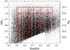 |
Fig. 1 Distribution of ΔBev, as defined in Eq. (1), as a function of redshift z for galaxies in the VIPERS sample. The red lines enclose the selected sub-samples of galaxies. The right-side vertical axis shows the values of the absolute magnitude MB for a fixed redshift z = 0.7. |
In Fig. 1 we present the distribution of rest-frame ΔBev as a function of redshift for the VIPERS galaxies. The left-side vertical axis shows the ΔBev value, whereas the right-side axis gives the absolute magnitude MB at the mean VIPERS redshift z = 0.7. As expected, due to selection effects, we progressively lose the faint population to higher redshifts, leaving only the brighter objects. In the present study we considered 12 volume-limited subsamples represented by the red boxes in Fig. 1. Each subsample is statistically complete, spans ΔBev = 0.5 magnitudes and has a redshift range Δz = 0.15.
2.3. CFHTLS imaging
The morphological analysis was based on the study of the 2D surface brightness profile of the VIPERS galaxies. To model the light profile of galaxies in the VIPERS PDR-1 we used CCD images in the i-band from eighteen W1 and eleven W4 CFHTLS fields covering 28 deg2 of the VIPERS project. While the VIPERS PDR-1 catalogue is based on the Terapix T0005 release, for the analysis of the structural parameters we use a more recent version of the CFHTLS data (i.e. T0006, Goranova et al. 2009). A full description of the CFHTLS data processing including calibration, stacking and mosaicing is provided in Mellier et al. (2008) and Goranova et al. (2009). The public data from Terapix T0006 are organised in 1° × 1° fields and have a pixel scale of 0.186″. The mean seeing, as parameterised by the Full Width at Half Maximum (FWHM) of stellar sources, depends on the filter of the CFHTLS images and is equal to 0.85″, 0.78″, 0.72″, 0.64″, 0.68″ in the u,g,r,i/y (the filter i broke in 2006 and it was replaced by a similar, but not identical filter, called y) and z-bands, respectively (Goranova et al. 2009).
To secure the quality of the derived morphological parameters, we used CCD tiles in the i photometric band where the mean FWHM is smallest. Objects were extracted by independently running SExtractor on the CFHTLS tiles in the T0006 release. This means that the centroid of photometric sources can be slightly different from the coordinates of the corresponding VIPERS spectroscopic objects. We associated spectroscopic and photometric sources on the basis of their relative (projected) distance, assuming a maximum matching radius equal to 1″. For 98.6% of the objects, the distance between the VIPERS galaxy (i.e. its position according to T0005) and the one in the T0006 release is less than 0.3″, and is larger than 0.5″ for only 0.3% of objects. Objects with distances larger than 1″ were excluded from the present analysis.
3. Rest-frame colours
3.1. Colour-based classification of galaxies
To probe the colour distribution of VIPERS galaxies we use the rest-frame (U−B) versus (B−V) colour-colour plot, based on the absolute magnitudes derived in Fritz et al. (2014).
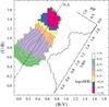 |
Fig. 2 Density of the VIPERS galaxies in the rest-frame (U−B) versus (B−V) colour–colour diagram. The contour lines show the galaxy density distribution in five equally spaced levels from 10% to 99% of the maximum value. The histogram shows the galaxy number density distribution projected along the line A−A connecting the two maxima of this distribution. The colours show the median sSFR 1/yr values of galaxies derived from SED fitting in seven equally spaced logarithmic bins. |
The isodensity contour lines presented in Fig. 2 show an evident bimodality in the rest-frame colours, with two well-separated peaks. We define the combined colour UBV by projecting the galaxy rest-frame colours along the A−A dashed line that connects the two density peaks of Fig. 2. In this way the separation of the red and blue populations is even more prominent than using the one-dimensional analysis, that is, based only on (U−B) or (B−V) rest-frame colours. The dashed line that defines the combined UBV rest-frame colour is described by the following equation:  (2)where U,B and V are absolute rest-frame magnitudes in the corresponding pass-bands. The angle θ = 58.08° is the slope of the A−A line crossing two maxima of the rest-frame colour density distribution, as shown in Fig. 2. The UBV colour thus allows for a better separation of two main galaxy populations. The UBV rest-frame colour separation of the two peaks along the UBV line is equal to 0.71, compared to 0.61 and 0.37 when it is projected on the (U−B) and (B−V) axes, respectively.
Figure 2 is colour coded by the median specific Star Formation Rate (sSFR is defined as the star formation rate per unit stellar mass of a galaxy) of galaxies inside a given small range of (U−V) and (B−V) colours. The sSFRs are derived via SED fitting. Values of constant sSFR are almost perpendicular to the line connecting the two colour peaks (A−A line), with values of sSFR steadily decreasing with UBV rest-frame colour along the line A−A. The correlation between the UBV colours and sSFR is therefore clearly evident, with blue colours corresponding to higher values of sSFR and red galaxies being mostly quiescent. It is also noticeable how this correlation is stronger than the one with (U−B) or (B−V) colours used independently. The local minimum of the UBV probability distribution corresponds to log (sSFR) ≈ 10-10−10-9.5 yr-1, which is in a broad agreement with the characteristic value for green valley galaxies selected in the NUVrK diagram (Davidzon et al. 2016). Therefore, even if in the following analysis we use the colour UBV, we note that this parameter can be considered a good proxy of sSFR.
3.2. Galaxy colour bimodality
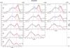 |
Fig. 3 UBV rest-frame colour distributions (black histograms) of VIPERS galaxies in different redshift (increasing from left to right) and luminosity (from top to bottom) bins. The blue and red curves represent the Gaussian components fitting the colour distribution of the two galaxy populations, and the vertical dashed lines mark the maxima of the Gauss functions. The solid brown line shows the sum of the two Gaussians. The central values and 1σ widths of the Gaussians for the blue and red galaxy populations are labeled in each panel, in the top left and right respectively. The number of galaxies considered in each bin is also shown in the bottom right of each panel. |
To investigate the dependence of the UBV rest-frame bimodality on galaxy luminosity and redshift we have computed the distribution of the combined rest-frame colour UBV defined in Eq. (2) in each of the subsamples shown in Fig. 1, that is, five equally-sized bins in ΔBev of width 0.5 mag and three bins in redshift, each of width 0.15 in z (0.50 <z ≤ 0.65, 0.65 <z ≤ 0.80 and 0.80 <z ≤ 0.95). The results are presented in Fig. 3. The bimodality is a persistent feature over the whole luminosity-redshift range explored. The shape of the PDF changes, however. The red population (the red line) is dominant at bright luminosities, whereas the blue population (blue line) becomes increasingly significant in the faintest magnitude bins. As already mentioned in Sect. 1, many studies have reported and described this colour bimodality in galaxies out to z ~ 2 (e.g. Strateva et al. 2001; Blanton et al. 2003; Baldry et al. 2004; Bell et al. 2004; Willmer et al. 2006; Faber et al. 2007; Blanton & Berlind 2007; Fritz et al. 2014).
The optical colour distribution is, in general, well modelled by the sum of two Gauss functions (Strateva et al. 2001; Baldry et al. 2004; Ball et al. 2008). Figure 3 also shows that the UBV rest-frame colour distribution is well approximated by the sum of two Gaussians (the brown curves), in agreement with previous results (e.g. Baldry et al. 2004). Similar results are also found in Ball et al. (2008) and González et al. (2009), for example.
The mean and the dispersion of each Gaussian component (the blue and red curves) depend on magnitude and redshift. The blue objects are characterised by a larger dispersion in colour than the red ones, which justifies the terms “blue cloud” and “red sequence”, generally used to characterise the two populations.
The local minimum is thought to be populated by objects that are evolving from star-forming to quiescent galaxies. We did not find a significant excess of objects between the two main galaxy populations with respect to the sum of the two Gauss functions, meaning that there is no statistical evidence of a third population of objects. This is at opposition with the results of other analyses which claim to find an excess of objects in the region between the two peaks (e.g. Wyder et al. 2007; Mendez et al. 2011; Schawinski et al. 2009; Coppa et al. 2011; Loh et al. 2010; Lackner & Gunn 2012; Brammer et al. 2009). This excess of galaxies is usually found in the distribution of several colour indices, such as U−B (Nandra et al. 2007; Yan et al. 2011), U−V (Brammer et al. 2009; Moresco et al. 2010) and NUV−r (Wyder et al. 2007; Fritz et al. 2014). In particular, Wyder et al. (2007) show that the NUV−r colour distribution is not strictly the sum of two Gaussians, and Coppa et al. (2011), using zCOSMOS data in the redshift range 0.5 <z< 1.3, reported a third galaxy population located between the blue and red populations. The lack of the third galaxy population located between two Gaussians peaks is possibly related to the narrow luminosity and redshift bins used in this study. The excess of galaxies with respect to the sum of the two Gaussians appears when using a coarser grid redshift or luminosity. Moreover, the UBV rest-frame colour, being an excellent proxy to sSFR, is more efficient at separating different galaxy populations and less prone to contaminating objects that could populate the intermediate colours.
While in the local Universe the colour–magnitude diagram is effective at dividing galaxies into different populations (e.g. Strateva et al. 2001; Baldry et al. 2004; Wyder et al. 2007), to study distant galaxies, it becomes important to consider how the selection depends also on galaxy luminosity and redshift (Bell et al. 2004). Exploring the effects of the luminosity and redshifts in the VIPERS sample, we reveal the systematic blueing of both the blue and red populations moving towards fainter magnitudes at fixed redshift (blue and red vertical lines in Fig. 3). Quantitatively, the blue cloud moves from UBV = 1.07 to 0.73 and the red sequence from UBV = 1.50 to 1.37 at z = [0.50,0.65] for values of ΔBev increasing from −1.5 to 1.0. Similar trends in the analysis of the u−r rest-frame colour have been found in the low redshift Universe by Ball et al. (2008) and Mendez et al. (2011) using the SDSS galaxy sample. Moreover, both populations in Fig. 3 evolve toward bluer colours when moving to higher redshifts.
The positions of the Gaussian maxima of the red and blue populations can be described by the following formalism:  where z is the redshift, ΔBev is the distance from the evolving characteristic luminosity as defined in Eq. (1), and UBVb and UBVr are the central positions of the blue and red galaxy distributions, respectively. The quoted errors on the coefficients were estimated through a bootstrap procedure using 1000 resamplings.
4. Sérsic index
4.1. Estimation of Sérsic parameters
To derive the surface brightness parameters of VIPERS galaxies, we have performed a 2D fit of the observed galaxy i-band light distribution with a PSF-convolved Sérsic model. We used the single component Sérsic (1963) profile given by the equation: ![Mathematical equation: \begin{equation} I(r)=I_{\rm e}\exp\left\{ -b_{\rm n} \left[ \left( \frac{r}{r_{\rm e}}\right)^{1/n}-1\right] \right\}, \label{sersic_eq} \end{equation}](/articles/aa/full_html/2017/02/aa28953-16/aa28953-16-eq113.png) (5)where re is the radius enclosing half of the total light of the galaxy, Ie is the mean surface brightness at re, and bn is a normalization factor, which is chosen in such a way that re corresponds to the half-light radius (Graham & Driver 2005). This parametrisation well describes the light distributions of elliptical, spiral and irregular galaxies (see e.g. Trujillo et al. 2001a). The detailed analytical properties of Eq. (5) are discussed by Ciotti & Bertin (1999), Trujillo et al. (2001b), and Graham & Driver (2005) for example.
(5)where re is the radius enclosing half of the total light of the galaxy, Ie is the mean surface brightness at re, and bn is a normalization factor, which is chosen in such a way that re corresponds to the half-light radius (Graham & Driver 2005). This parametrisation well describes the light distributions of elliptical, spiral and irregular galaxies (see e.g. Trujillo et al. 2001a). The detailed analytical properties of Eq. (5) are discussed by Ciotti & Bertin (1999), Trujillo et al. (2001b), and Graham & Driver (2005) for example.
There are many codes in common usage that model the observed galaxy shapes, such as GIM2D (Simard et al. 2002), BUDDA (de Souza et al. 2004), GASPHOT (Pignatelli et al. 2006), GALFIT (Peng et al. 2002) and GAMA-Sigma (Kelvin et al. 2012), for example.
We used the code GALFIT (Peng et al. 2002) to perform the fit. The fitting procedure of GALFIT provides the value of the semi-major axis (ae), the axial ratio (b/a) of the profile, from which the circularised effective radius ( ), a standard parameter used in the studies of the galaxy morphology is derived, the Sérsic index n, and the apparent magnitude of the modeled galaxy.
Many GALFIT wrappers to automatise galaxy fitting procedures are publicly available, such as GALAPAGOS (Häußler et al. 2011), PyMorph (Vikram et al. 2010) and GAMA-Sigma (Kelvin et al. 2012). We decided, however, to develop dedicated software combining galaxy profile fitting by GALFIT and the PSF determination to have the parameters used in the galaxy profile estimation fully under control.
We used the CFHTLS-T0006 images of VIPERS targets, and divided each 1° × 1° tile into postage stamps centred on each VIPERS galaxy (see some examples in Fig. 4). To define the size of the postage stamps, we rely on the SExtractor parameters, which describe the ellipse associated to a given i-band detection, namely RK (KRON_RADIUS), A, B (A_IMAGE, B_IMAGE) and θ (THETA_IMAGE). The centre of each postage stamp coincides with the centroid of the SExtractor ellipse, while its sides (Δx and Δy) are four times larger than the projected total dimension of the ellipse on the x and y axis, that is, 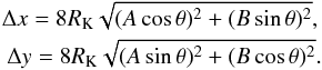 (6)These sizes ensure that each postage stamp has sufficient object-free pixels to estimate the background emission, which plays an important role in galaxy image fitting. Similar image sizes are used by other authors (e.g. Häussler et al. 2007; Kelvin et al. 2012).
There are two main approaches to estimating the level of background emission. In the first procedure the background is characterised independently of the analysis of the target object, computed a priori, from an annular region surrounding the galaxy, for example (Barden et al. 2005; Häussler et al. 2007; Guo et al. 2009; Fritz et al. 2009; Fritz & Ziegler 2009). In the second method the background is a free parameter that can vary during the GALFIT fitting (Mosleh et al. 2013; Cassata et al. 2011). The Sérsic parameters presented in this paper were obtained using this second approach, that is, when the background is a free parameter. When the area of the postage stamp is approximately 10 times larger than the target galaxy and the sky-background variance is uniform, the two methodologies to estimate the background are equivalent (Cassata et al. 2011; Mosleh et al. 2013). These conditions are satisfied in our data.
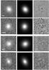 |
Fig. 4 Four examples of the GALFIT image approximation procedure. Left column: postage stamps with observed galaxies; middle column: best-fit PSF-convolved Sérsic model to each galaxy; right column: residual images. The small horizontal bars in the left column correspond to 1″. |
Postage stamps centred on each galaxy were extracted from the CFHTLS tiles, and SExtractor was run to detect all of the objects contained therein. In the fitting procedure, all of the other objects within the postage stamp are masked, unless the aperture ellipse of a secondary object, increased by a factor 1.5, overlaps with that of the main target. In that case, the two (or more) photometric sources are fitted simultaneously to get the best values of the Sérsic profile parameters.
The proper values of the initial parameters play an important role in the non-linear approximation. The values MAG_AUTO, FLUX_RADIUS, A_IMAGE, B_IMAGE, THETA_IMAGE obtained by SExtractor were used as a first guess of re, position angle, ellipticity, and magnitude in GALFIT. In the absence of an estimate of the Sérsic index n in the SExtractor output, the initial value of this parameter in GALFIT fit was set to n = 1.7 for all galaxies. A similar methodology has also been applied in other studies (e.g. Häussler et al. 2007; Kelvin et al. 2012)
To convolve the Sérsic model, GALFIT requires a local point spread function (PSF) for each postage stamp. In our analysis we used the Moffat function (Moffat 1969), that combines simplicity, accuracy and allows us to easily reconstruct the anisotropy of the CFHT field of view. In the first step, the isolated stars were selected from the SExtractor output from each 1° × 1° CFHTLS tile and the Moffat (1969) function was fitted to each star. Then, the values of the estimated Moffat function parameters were approximated as a function of the star position in each CFHTLS tile. To ensure numerical stability we applied the 2D Chebyshev base: cos(narccos(x)) instead of the algebraic polynomial one: xn, where n = 0,1,2, etc. The procedure allows us to generate the PSF at the central position of each studied galaxy. A detailed description of the PSF construction is given in Appendix B.
Figure 4 shows some examples of the fit performed by GALFIT for VIPERS galaxies. The original image of the galaxy, the best-fit PSF-convolved Sérsic model of each galaxy, and the residual map are shown. More details about our morphological analysis and the reliability of GALFIT results are presented in Appendix A. Briefly, we added 4000 artificial galaxies to the CFHTLS images with structural parameters generated from the Sérsic indices, magnitudes and effective radii obtained by GALFIT for a randomly-selected subset of the VIPERS galaxies used in this analysis. From these tests, we estimate uncertainties in our measurements in the magnitude range from 19 to 22.5 mag, of n of | Δn | /n = 0.16 at the 68% level, and 0.33 at the 95% level (i.e. for 95% of galaxies in our sample), while the effective radii are accurate to within 4.4% and 12% for 68% and 95% of our sample, respectively. Our tests also confirm that any bias in the n measurements is negligible.
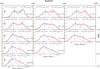 |
Fig. 5 Sérsic index distribution (black histograms) for different redshift (from left to right) and ΔBev luminosity bins (from top to bottom). The blue and red solid lines show the Gaussian fits to the disc-like and spheroid-like populations, respectively. The vertical dashed lines mark the central values of each Gaussian. The sum of the two Gaussian fits is shown as a solid brown line. The central values ⟨ n ⟩ of the Gauss functions, their 1σ widths, and the total number of galaxies in each bin are shown in each panel. |
The angular size of the VIPERS galaxies at z = [0.5,1] is of the order of a few arcseconds and even in the best quality CFHTLS i-band images used in this study, where the mean value of the FWHM is as small as ~0.6″, it is difficult to detect the internal structure of these objects. Almost all of them exhibit a smooth light profile.
When discussing the uncertainties of the fitted Sérsic profile parameters it should be noted that the χ2 criterion is not optimal to compare different models of the light distribution of noisy galaxy images (Peng et al. 2002). Nevertheless, the χ2 criterion is commonly used in similar studies (e.g. Morishita et al. 2014).
During the fitting procedure, GALFIT reported a converge problem for some galaxies: for this reason 5707 (12%) of them were removed from the present work. Moreover, to analyse the galaxies with the best quality Sérsic function parameters, we selected only the objects with reduced χ2 ( ) values smaller than 1.2. Even though the χ2 is not the optimal criterion to compare different models of the light distribution of noisy galaxy images (Peng et al. 2002), it has been used in similar studies (e.g. Morishita et al. 2014). In fact, from the simulations presented in Appendix A we detected an increase of the fractional error on the Sérsic index n for increasing values of . We preferred to remove the 4% of galaxies in the high-end tail of the distribution in order to have a very high quality sample, the vast majority of fits producing values in the range 0.9−1.15. We also discarded 261 objects with n< 0.2: low values of the Sérsic index imply a lower accuracy in the approximation of the Sérsic bn normalisation factor (Ciotti & Bertin 1999) and introduce a small bias on the distribution of the disk-like profiles, but are negligible when compared to the error bars of the fitted Sersic index. Moreover, small values of n< 0.2 are unphysical. Similar low-n cuts are commonly used in other studies. Finally we obtained our sample, constituting 38 620 galaxies. The volume-limited sample of objects presented in Fig. 1 consists of 22 131 galaxies.
4.2. Sérsic index bimodality
Figure 5 shows the Sérsic index distribution of VIPERS galaxies in the same luminosity and redshift bins as used in Sect. 3.2 for the UBV colour. Since the Sérsic index, n, appears as an exponent in Eq. (5) defining the Sérsic profile (Driver et al. 2006, 2011), a logarithmic-spaced x-axis is used to optimise the analysis and visualisation of the wide range of n values.
Similarly to the UBV histograms shown in Fig. 3, the Sérsic index distribution is bimodal in many of the redshift-luminosity bins. We thus fit each Sérsic index distribution as a sum of two Gauss functions in log n, with one Gaussian component considered to represent the disk-like population (blue curves), and a second to represent the spheroid-like galaxy population (red curves). The sum of the two Gaussian fits (solid brown curves) well describes the Sérsic index distribution at all redshifts and luminosities explored here. Even though, for galaxies fainter than the characteristic luminosity of the LF, that is, ΔBev> 0.0, the global distribution is not evidently bimodal, it is well reproduced by the sum of the two Gauss functions.
The vertical blue and red dashed lines in Fig. 5 show the central values of the two Gaussian components for each redshift and luminosity bin. Comparing the locations of these lines from panel to panel, we see that the mean Sérsic indices of both disk-like and spheroid-like galaxy populations vary systematically with luminosity and redshift. In particular, both disk-like and spheroid-like populations become increasingly concentrated with increasing luminosity and decreasing redshift.
We find that the best two-dimensional linear fit of these positions in the redshift z versus ΔBev luminosity plane is well described by the following equations:  where ΔBev is the luminosity given by Eq. (1) and nd and ns are the mean Sérsic indices of the disc-like and spheroid-like galaxy populations. The errors of the best-fit coefficients were estimated by a bootstrap procedure using 1000 resamplings.
In principle, the Sérsic index can vary with rest-frame wavelength. The analysis presented in this paper is based on the optical i-band images, which correspond to rest-frame 510 nm at z ~ 0.5 and to 348 nm at z ~ 1.2. One way to account for this rest-frame change would be to use images obtained through different filters for galaxies at different redshift ranges. However, the CFHTLS images made in filters u,g,r,z are of lower quality than i-band images which introduces additional noise, higher than a possible effect of the expected correcting factor. Taking this into account, we try to examine a possible effect of this morphological K-correction based on the measurements of local galaxies. Kelvin et al. (2012) and Vulcani et al. (2014) investigated this property in the nearby galaxies of GAMA survey at z< 0.25. Using different galaxy selection criteria, both based on log (n) and u−r colour, they found that the Sérsic index value increases with wavelength, and that, for disk-like galaxies, this relation is steeper than for spheroidal ones. One might then ask if the redshift evolution of the Sérsic index given by Eqs. (7) and (8) could be explained by the change in the rest-frame wavelength. The centre of the i-band filter is positioned at λz = 0 = 765 nm and is shifted in the observed redshift range from λz = 0.5 = 510 nm to λz = 1.0 = 383 nm. According to Eqs. (10) and (11) from Kelvin et al. (2012), in such a range of wavelength the value of the Sérsic index of the disk-like galaxies might change from nz = 1.0 = 0.89 to nz = 0.5 = 1.10, whereas for the spheroidal galaxies it would change from nz = 1.0 = 2.79 to nz = 0.5 = 3.03. However, the evolution of the Sérsic index both for disk-like and spheroidal VIPERS galaxies, given by Eqs. (7) and (8), is faster than expected from the change of the observed rest-frame wavelength only. For late-type galaxies the slope of this relation is equal to −0.82, whereas Kelvin et al. (2012) prediction gives –0.42. For the early-type objects our slope and the slope given by Kelvin et al. (2012) are equal to –1.26 and –0.52, respectively. Thus, the change of the rest-frame wavelength with redshift can only partially explain the observed changes of the Sérsic index. Thus, a large part can be attributed to the genuine galaxy evolution in the redshift range z = [0.5,1.0].
The Sérsic index n = 1, commonly used to model the light profile of the disk-like galaxies, is well inside the range [0.81, 1.11] spanned by the average Sérsic indexes measured within the analysed redshift-luminosity space limits. For spheroid-like galaxies we find mean values in the range [2.42, 3.69], lower than the typical value used to describe nearby elliptical galaxies (i.e. n = 4, see de Vaucouleurs 1948). Other authors have reported similar Sérsic indices for early-type galaxies; ⟨ n ⟩ = 3.0 (D’Onofrio 2001), ⟨ n ⟩ = 3.3 (Padmanabhan et al. 2004), and n> 2.5 (Eales et al. 2015; Griffith et al. 2012), for example. Moreover, the tests presented in Appendix A ensure that the Sérsic parameters we obtained are reliable and that the bias in the estimate of n is negligible for all the redshift and luminosity bins considered in this analysis.
5. Comparison with the literature
Previous studies have shown that the Sérsic index of galaxies depends on both their absolute magnitude and redshift (e.g. Graham & Guzmán 2003; Tamm & Tenjes 2006; van Dokkum et al. 2010, 2013; Patel et al. 2013; Buitrago et al. 2013). To compare our results with other works, Eqs. (7) and (8) are combined with Eq. (1) to obtain the following relations:  where the dependence on absolute magnitude is made explicit. The relation between galaxy luminosity and Sérsic index has been reported in many studies for spheroid-like galaxies (e.g. Young & Currie 1994; Graham & Guzmán 2003; Ferrarese et al. 2006). Moreover, a link between structural parameters and luminosity has also been studied by Cross et al. (2004) for E/S0 galaxies in the redshift range from z = 0.5 to 1. Equations (9) and (10) show that fainter disc and spheroidal galaxies have lower values of the Sérsic index than the luminous ones and that this relation depends on redshift.
The dependence of Sérsic index on redshift has been analysed in many studies (e.g. Tamm & Tenjes 2006; van Dokkum et al. 2010, 2013; Patel et al. 2013; Buitrago et al. 2013). Figure 6 shows the Sérsic index-redshift relations for both disc-like and spheroid-like populations within VIPERS for three absolute magnitude values and the comparisons with previous studies. In the following sections we analyse the comparison for the two classes of galaxies in detail.
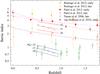 |
Fig. 6 Sérsic index – redshift relation: VIPERS results are presented as red and blue solid lines for spheroid- and disc-like galaxies, respectively, for three values of B-band absolute magnitude. Patel et al. (2013)’s results for quiescent and star-forming objects with log (M/M⊙) > 10.5 are shown as red filled and empty circles and dashed magenta and blue lines. The relation found by van Dokkum et al. (2010) for a constant co-moving number density sample is plotted in brown (short-dashed line and triangles). Buitrago et al. (2013)’s results for a sample visually classified into early- and late-type galaxies is shown as orange filled and empty diamonds, while disc-galaxies measured by Tamm & Tenjes (2006) are represented by green squares. The dot-dashed lines show n(z) relation corresponding to the disk-like and spheroidal galaxies, only for MB = −21 mag, obtained from the 2D analysis presented in Sect. 6. |
5.1. Spheroid-like galaxies
Patel et al. (2013) computed structural parameters of massive galaxies in high-resolution HST imaging from the CANDELS and COSMOS surveys, and measured the evolution of the Sérsic index of galaxies in the redshift range 0.25 < z < 3, after splitting them into quiescent and star-forming populations on the basis of their rest-frame UVJ colours.
The solid red lines show the Sérsic index-redshift relations for spheroid-like populations described by Eq. (10) for three values of B-band absolute magnitude. The solid red circles in Fig. 6 show the median Sérsic indices for quiescent galaxies with log (M/M⊙) > 10.5 in four redshift bins, while the orange dashed line indicates their best-fit Sérsic index-redshift relation over the redshift range 0 < z < 2.5 of the form n ∝ (1 + z)− 0.50( ± 0.18). The exponent of this relation is consistent with our fit, n ∝ (1 + z)-0.64, that we obtain for our brightest (MB = −22) spheroid-like galaxies, which also fulfill their criterion log (M/M⊙) > 10.5.
van Dokkum et al. (2010) measured the Sérsic index parameter from stacked rest-frame R-band (observed J,H-band) images from NEWFIRM Medium Band Survey. They selected a sample at a given constant cumulative number density, which results in their use of a stellar mass limit which evolves with redshift. The stellar mass limit of their selection at our mean redshift z ~ 0.7 is log (M/M⊙) > 11.35 and does not vary considerably (<0.07 dex) in the redshift range we are exploring, 0.5 < z < 0.95. At these large stellar masses the galaxy population is dominated by quiescent objects. Rather than fitting Sérsic profiles to each individual galaxy and measuring the mean of the distribution, van Dokkum et al. (2010) created deconvolved, stacked images of massive galaxies within bins of redshift, and fitted Sérsic functions to the stacked radial surface density profile, the results of which are shown as brown triangles in Fig. 6. They measure a best-fit evolution for the Sérsic index of the form n = 6.0 × (1 + z)-0.95 over the range 0 <z< 2 0<z<2, presented with the brown line in this plot. The redshift evolution is faster than in Patel et al. (2013), perhaps reflecting the contamination by non-quiescent objects or systematics in measuring Sérsic indices from stacked images, but is in good agreement with our results in the common z-range.
Buitrago et al. (2013) estimated quantitative and visual morphologies from HST images of a sample drawn from the DEEP2 and GOODS surveys, combined with a local sample based on SDSS imaging. Their sample of massive log (M/M⊙) > 11 galaxies was then subdivided into early- and late-type galaxies on the basis of the visual classification. The mean Sérsic indices of visually-selected early-types in bins of redshift are displayed as orange diamonds, and show the same gradual increase in n with time, albeit systematically shifted to higher Sérsic index values by Δn ~ 1.5. Despite the different selection criteria, the evolution of the Sérsic index for bright spheroid-like galaxies is in good agreement with the relations found in the literature for massive quiescent galaxies.
5.2. Disk-like galaxies
The Sérsic index-redshift relation for disc-like galaxies given by Eq. 9 is represented in Fig. 6 with dark blue lines, and for MB = −22 mag can be written as nd = 1.65(1 + z)-0.98. The dependence of the n-redshift relation on absolute magnitude is smaller for disc-like- than for spheroid-like galaxies, while its evolution with cosmic time is faster for disc-like galaxies than for spheroid-like ones.
Patel et al. (2013) and Buitrago et al. (2013) found similar, decreasing trends. However, their relations are significantly offset from our results by Δn ~ 1, probably reflecting the fact that they used selection criteria very different from ours (i.e. star-forming galaxies in Patel et al. 2013 and very massive visually classified late-type galaxies in Buitrago et al. 2013). In particular, we found that the characteristic stellar mass of our disc-like sample, estimated from the mass-luminosity relation, corresponds to a selection of stellar masses smaller than log (M/M⊙) = 10.5.
For a much more meaningful comparison we turned to the Tamm & Tenjes (2006) sample who measured the Sérsic profile of 22 galaxies in the HDF-S using a selection similar to ours, as they have only considered disk-like galaxies (with n< 2) in absolute magnitude range −17 <MB< −22. It is therefore reassuring that theirs results are consistent with ours, as shown in Fig. 6, although their sample contains only 22 galaxies.
Comparing our results with previous work, we find, in general, a good agreement of the evolution of the Sérsic index for spheroid-like galaxies with the ones for quiescent and early-type galaxies. Instead, galaxies defined as star-forming are characterised by larger values of Sérsic index when compared to disk-like ones.
6. Sérsic index-colour distribution
In Sects. 3.2 and 4.2 we independently analysed the UBV rest-frame colour and the logarithm of the Sérsic index n of the VIPERS galaxies as a function of the redshift z and ΔBev luminosity. Both parameters show a bimodal distribution. Using the local galaxy sample of the Millennium Galaxy Catalogue, Driver et al. (2006) showed not only that both colour and Sérsic index are characterised by bimodal distributions, but that two well-separated populations exist on the u−r rest-frame colour versus log (n) plane. A similar method has been proposed by Kelvin et al. (2012) to study the morphological properties of galaxies in the GAMA survey.
To investigate whether this is still true at high redshift we have repeated the Driver et al. (2006) analysis in each of our subsamples. The results are shown in Fig. 7. The colours in each surface density map of this plot are normalised to have values in the range 0–1, so that 1 (dark red colour) is the peak density in each bin. The joint probability distribution of UBV rest-frame colour and Sérsic index n is clearly bimodal in all panels, with two well-separated peaks and indicates the presence of two different populations that we identify with early- and late-type galaxies.
The plot shows that the distribution of the late-type galaxies are centred at the Sérsic index value n ≈ 1 and the rest-frame colour UBV ≈ 0.8, while those of the early-type galaxies are centred at UBV ~ 1.4 and 2.5 <n< 4. The latter peak appears somewhat elongated along the n-axis and moves towards larger values of the Sérsic index (from n ~ 2.5 to 4) with cosmic time, that is, galaxies become more concentrated at lower redshift. The two peaks are separated by the local minimum located at UBV ~ 1.2, corresponding to sSFR 10-10 yr-1 (see Fig. 2); a value that is often used to separate active from passive objects (e.g. Davidzon et al. 2016). From these plots we see that a more effective separation can be made using the combined Sérsic index n and UBV rest-frame colour information.
We fitted the joint probability distribution of Sérsic index and UBV colour in each redshift-luminosity bin with the sum of two 2D-Gaussians. The iso-density contour lines are separated in steps of 0.2 times the maximum surface density value. The dashed circle around each peak shows the 0.5σ level of each 2D-Gaussian.
We do not include a covariance term for the Gauss functions in order to avoid artificially creating apparent correlations between UBV and n within the single populations due to the presence of the second population.
In addition to the dominant populations of early- and late-type galaxies, Fig. 7 shows that a fraction of blue galaxies have large values of the Sérsic index (n ≳ 2), while, conversely, some red galaxies have a Sérsic index n ≈ 1, typical of disc-like objects. We postpone a thorough investigation of these peculiar objects to a future analysis.
Moreover, Fig. 7 gives us information on the galaxy morphological type fraction in each luminosity/redshift bin. It shows that the most luminous bins are dominated by early-type galaxies, whereas the late-like galaxies dominate the less luminous sub-samples.
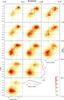 |
Fig. 7 UBV rest-frame colour vs. Sérsic index n distribution. Each panel shows the colour–coded galaxy surface density distribution map of the VIPERS galaxies in each redshift and ΔBev luminosity bin. The colour bar presented in the bottom right corner gives the normalised galaxy surface density. The contour lines show the density values in steps of 0.2 obtained from the two Gaussians bivariate fitting procedure. Blue and red dashed lines show the 2-dimensional model given by Eqs. (11)–(14). Crosses identify the positions of the centre maximal surface density distribution of the given galaxy population. The dashed lines around the peaks show the value of 0.5σ of the Gaussian fit. The histograms present the galaxy distributions projected on the Sérsic index and UBV colour axes, at the bin z = [0.65,0.80] and ΔBev = [0.5,0.0]. |
6.1. Early-type galaxies in the n-UBV plane
The galaxy surface distributions presented in Fig. 7 show that the positions of early- and late-type galaxy populations change with both redshift and luminosity.
Fitting the sum of two 2D Gauss functions to the distributions in each bin we obtain the positions of the population centres (log (n), UBV). Using these positions we determined the empirical relation connecting the galaxy population centre with ΔBev and redshift. Our results in Sects. 3.2 and 4.2 showed that the UBV rest-frame colour and the Sérsic index log (n) are well reproduced by a linear dependence on redshift and luminosity. We thus fit the position of the early-type galaxy population centre (log (ne),UBVe) in Fig. 7 with a two-dimensional linear function, obtaining the following set of equations describing the central position of this galaxy population as a function of redshift and luminosity:  where ΔBev is given by Eq. (1). The errors of the fitted coefficients were estimated via a bootstrap procedure using 1000 resamples.
The relations given by Eqs. (11) and (12) were used to compute the central UBVe and ne values for the early-type galaxy populations as a function of redshift and luminosity, shown in Fig. 7 as red dashed lines. The crossing points of these lines correspond to the position of the maxima described by the Eqs. (11) and (12), whereas the crosses show the surface density maxima of early-type galaxy population in each bin.
Comparing these positions with the shape of the higher density contour lines and the 0.5σ widths of the 2D Gaussian fits (marked as dashed ellipses) we find that the simple linear approximation given above accurately predicts the observed peak position of the early-type galaxy population. The mean distance between the maxima positions from data and the linear model is smaller than 0.1σ.
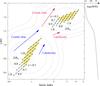 |
Fig. 8 UBV rest-frame colour versus Sérsic index log (n) relation of late-type (lower left corner) and early-type (upper right corner) galaxies. Dots indicate redshift from z = 0.5 to 1.0 in increments of 0.1. Black solid lines connect the values of ΔBev from −1.5 to 1 in 0.5 magnitude increments. The arrows show the direction of the redshift and luminosity galaxy evolution. The right plot presents the UBV colour versus sSFR relation. The 0.2 dex background contour lines show the bivariate number density of all studied VIPERS galaxies in our sample (0.5 <z< 0.95). The yellow coloured regions mark the analysed redshift and luminosity limits, as presented in Figs. 1 and 7. |
6.2. Late-type galaxies in the n-UBV plane
The same procedure was also applied to the late-type galaxy distributions. The following set of equations describes the central position (UBVl, log (nl) of the late-type galaxy population as a function of redshift and luminosity:  where ΔBev is given by Eq. (1). The UBVl and nl positions of the late-type galaxy population as a function of redshift and luminosity are derived similarly to early-type galaxies and presented as blue dashed lines in Fig. 7. The crossing points of these lines determine the maxima position described by Eqs. (13) and (14). The plot shows that our linear model accurately reproduces the positions of galaxy density maxima, with the distance from the maxima computed from data being smaller than 0.1σ.
6.3. Comparison of 1D to 2D approximation
In Sects. 3.2 and 4.2 we focused our attention on the 1D distributions of the Sérsic index and UBV rest-frame colour. It is worth comparing those results with the ones obtained from the 2D approximation. We find that both approaches give almost the same results for the UBV rest-frame colour position of the galaxy population centres. The 1D relations given by Eqs. (3) and (4) and the 2D ones presented by Eqs. (11) and (13) are consistent with each other within ±1σ of the fitted parameters.
Some significant differences occur, however, in the approximation of the Sérsic index log (n) positions. The coefficients representing the redshift dependence in the 1D relations given by Eqs. (7) and (8) and the 2D relations presented by Eqs. (12) and (14) are different, with the redshift dependence in the 1D representation being significantly shallower than that obtained with the 2D analysis. The origin of this difference is evident when comparing Figs. 7 and 5: the 2D galaxy distribution efficiently separates both galaxy populations for all ΔBev luminosity and redshift bins. In contrast, in the 1D projection of the Sérsic index log (n), these distributions partially overlap each other, especially for the less luminous disc- and spheroid-like galaxy populations, as clearly seen in the histograms presented in Fig. 5. Because of this, the results obtained with the 2D approach are much better determined and more robust than those obtained with the 1D analysis.
The Sérsic index evolution obtained from the 1D and 2D analyses can be compared, making use of Fig. 6 again. The dot-dashed black lines located in the regions of the disk-like and spheroidal galaxies show the n(z) relation at MB = −21 mag from the 2D approach given by Eqs. (12) and (14), respectively. Comparing these results with those obtained from the 1D analysis shown in the same plot as the solid blue and red lines, we find a steeper Sérsic index evolution in the 2D approach for both galaxy populations. In the 2D approach, the Sérsic index-redshift relation is well approximated by n ∝ (1 + z)-1.08 for late-type galaxies and by n ∝ (1 + z)-1.47 for early-type galaxies. The values of the exponents indicate a faster Sérsic index evolution with cosmic time than reported in previous works based only on the Sérsic index or rest-frame colour galaxy selection (e.g. Tamm & Tenjes 2006; van Dokkum et al. 2010, 2013; Patel et al. 2013; Buitrago et al. 2013). The galaxy type classification based on the 2D distribution of the Sérsic index versus UBV rest-frame colour allows us to better select galaxies belonging to the early and late-type galaxy population. In this way the method presented in this paper allows us to study in detail the morphological properties of galaxies belonging to the early and late-type galaxy populations.
7. Sersic index-UBV colour coevolution
The analysis presented in the previous sections provides a quantitative description of the Sérsic index-UBV colour relation and its dependence on redshift and galaxy luminosity. Figure 8 makes use of Eqs. (11)–(14) to present these dependencies on the Sérsic index versus UBV colour plane. Dots represent values given by the equations presented in the previous sections, for redshift from z = 0.5 to 1.0 in steps of 0.1, and black lines connect points corresponding to the fixed values of ΔBev ranging from –1.5 to 1.0 in increments of 0.5 mag. Contour lines represent the galaxy surface density of the whole VIPERS galaxy sample studied in this paper, in steps of 0.2 dex. The coloured regions highlight the redshift and luminosity limits presented in Figs. 1 and 7. The blue and red arrows indicate the change of values of UBV and Sérsic index log (n) as a function of redshift and luminosity. In Sect. 3.1 we show that the UBV rest-frame colour is well correlated with the sSFR. The approximate relation of UBV colour versus sSFR is presented on the right-hand side of Fig. 8.
The UBV rest-frame colour versus log (n) diagram allows us to make a division, at the intermediate redshift z ≈ 0.7, between the late-type galaxies (presumably, disk-like, blue and mostly star-forming) with UBV< 1.2 and n< 1.5 and early-type galaxies (presumably, spheroidal, red and mostly quiescent) for which UBV> 1.2 and n> 1.5. The UBV versus n plot also offers a possibility to separate two galaxy populations using a line perpendicular to the connection between the maxima and passing through the minimum along the same line. A similar method has been proposed by Kelvin et al. (2012).
Figure 8 visually connects four galaxy parameters and allows us to present the coevolution of the properties of galaxies belonging to the early- and late-type classes. In fact, from this figure, it is already clear that the evolution of the relation between UBV and n is markedly different for early- and late-type galaxies, similar to the findings of other studies (e.g. Blanton et al. 2003). We also find that the Sérsic index n of both main morphological galaxy types (disk-like and spheroidal) increases with both their luminosity and cosmic time. This result is consistent with observations and numerical simulations (e.g. Conselice 2003; Conselice et al. 2005; Treu et al. 2005; Bundy et al. 2005; Brook et al. 2006; Aceves et al. 2006; Hopkins et al. 2007).
7.1. Early-type galaxies
The results presented in the previous sections allow us to give a general overview of the colours and structural properties of early-type galaxies (ETGs). Figure 8 shows explicitly the effect of evolution and luminosity on the colours and structural properties of ETGs. Firstly, it confirms that ETGs simultaneously become redder and more concentrated with both cosmic time and increasing luminosity (presumably correlated with stellar mass) (Trujillo et al. 2001b; Graham & Guzmán 2003; Tamm & Tenjes 2006; van Dokkum et al. 2010, 2013; Patel et al. 2013; Buitrago et al. 2013). However, the effects of increasing luminosity and cosmic time on early-type galaxies act in different directions. This means that we cannot take a low-luminosity, early-type galaxy at z = 1.0 and simply wait a few Gyr for it to become as red and as concentrated as its high-luminosity counterpart was at z = 1.0. At z = 1.0, we see that a low-luminosity (ΔBev = + 1.0) red galaxy is 0.10 mag bluer in UBV and 0.6 times less concentrated than its 10 times more luminous (ΔBev = −1.5) red counterpart.
Following a galaxy evolutionary track, we see that while a galaxy can rapidly redden to match its high-luminosity counterpart by z = 0.63, over the same time-scale it only marginally increases its concentration by a factor equal to 1.17, that is, only a quarter of the amount needed to match that of high-luminosity ETGs at z = 1.0. Indeed, even at z = 0 (assuming an extrapolation of the linear trends) its Sérsic index will not have increased sufficiently.
Low-luminosity early-types are known to have later formation epochs and more extended bursts of star formation than their high-luminosity counterparts and have delayed star formation histories (e.g. Thomas et al. 2005). The delayed star formation can also be seen tentatively from the plot in Fig. 8, where low luminosity galaxies seem to have, on average, larger values of sSFR than brighter ones at a fixed redshift.
The results presented here confirm that while it is possible to account for this delay by matching low-luminosity ETGs observed at lower redshifts to higher-mass ETGs seen at earlier epochs, and to first order to have stellar populations of equivalent ages (although the metallicities will differ), the lower-luminosity ETGs will still have quite different structural properties, being much less concentrated at fixed stellar age. This fundamental difference likely reflects the less active merger history of lower-luminosity (mass) ETGs (e.g. Rodriguez-Gomez et al. 2016; Lacey & Cole 1993; Aceves et al. 2006; De Lucia et al. 2006), meaning they cannot build up the more extended stellar halos of high-mass ETGs.
If we assume that the increase in n is due to major mergers (e.g. Aceves et al. 2006) and the continual accretion of material onto the outskirts of the galaxy, the trends of Fig. 8 suggest that low-luminosity ETGs do not undergo sufficient minor mergers at late epochs to “catch up” the much more active merger history of high-mass ETGs at z> 1.
7.2. Late-type galaxies
At first sight, Fig. 8 suggests that late-type galaxies (LTGs) show very similar trends to early-type, becoming simultaneously redder and more concentrated, both with cosmic time (decreasing z) and increasing luminosity. Moreover, the evolution from z = 1 to z = 0.5 in the UBV vs. log (n) plane is similar in magnitude and direction to that of the early-type population, leaving the separation between the two populations virtually unchanged, as is presented in Fig. 7. Hence, the bimodality appears to neither strengthen nor weaken with time, at least for the redshift range studied here.
Interestingly however, the relative impacts of time and luminosity on UBV colour and log (n) appear to have flipped in comparison to those seen among the ETGs. The concentration of LTGs is most dependent on cosmic time, while UBV colour increases mostly with luminosity. At z = 1.0, a low-luminosity LTG (ΔBev = + 1.0) is 0.375 mag bluer and 1.6 times less concentrated than its 10 times more luminous counterpart (ΔBev = −1.5). By following its evolutionary track, it is able to change its structure sufficiently rapidly to match the Sérsic index of its high-luminosity counterpart by z = 0.41, but over this same time period it is only expected to become 0.18 mag redder, half of that required to match the UBV colour of the high-luminosity LTG at z = 1.
Given the well known systematic decline in specific-SFRs among LTGs over 0 <z< 1, in which both high- and low-luminosity (stellar mass) spirals see their star formation drop exponentially and in step (e.g. Noeske et al. 2007; Zheng et al. 2007), it is interesting to note that their structural parameters are changing more rapidly than their colours, while UBV colour is more dependent on luminosity. It should in fact be easier to make a spiral galaxy redder by reducing star formation, than an early-type galaxy, as the response to a reduction in star formation is greatest when the galaxy is initially blue (see e.g. Fig. 2 and the right-hand plot of Fig. 8). One explanation could be that the large change in UBV colour with luminosity among LTGs more greatly reflects the increased reddening due to dust in massive spirals rather than a decrease in specific-SFR.
Theoretically, it is expected that the bulge fraction of merger remnants increases with the decreasing gas fraction of the progenitors (e.g. Robertson et al. 2006; Hopkins et al. 2009). The higher luminosity (mass) disk-like galaxies have a higher bulge fraction due to major- and intermediate-mass ratio mergers. The dense luminous part of galaxies is undisturbed during this process and luminous material dominates the central regions of mergers’ remnants (Barnes & Hernquist 1992), and their Sérsic index value increases, as shown in this study.
8. Summary
In this paper we present the coevolution of galaxy morphological properties and colours over the redshift range from z = 0.5 to 1, combining high-quality imaging data from the CFHT Legacy Survey with the large number of redshift and extended photometry from the VIPERS survey. We used this new dataset to investigate the coevolution of galaxy Sérsic index and UBV rest-frame colour. The galaxy structural parameters were measured by GALFIT fitting the Sérsic profile to the i-band CFHTLS T0006 images. To do this, the PSF of the images was precisely estimated and approximated over the whole of each 1° × 1° tile. The resultant parameters were carefully tested using a set of different methods, which confirms the good quality of the fits and reliability of their fitted values. Our results can be summarised as follows:
-
We find a clear bimodality of the UBV rest-frame colour and Sérsic index distribution, very well approximated by a sum of two Gaussians over the explored redshift and luminosity ranges. We parametrised the position of the two maxima in UBV and n distributions as a function of luminosity and redshift. This parametrisation allow us to analyse the colours and structural parameters of the red and blue, or the spheroidal and disk-like galaxies based on their location in the luminosity-redshift space.
-
The 1D and 2D methods show the evident bimodality both of the UBV rest-frame colour and Sérsic index distribution up to redshift z = 1.
-
The combination of the UBV rest-frame colour and Sérsic index n, as a function of redshift and luminosity, leads to a precise statistical description of the structure of galaxies and their evolution. Our method of analysis connects four galaxy parameters, that is, UBV colour, Sérsic index, luminosity and redshift, and allows us to present the coevolution of the properties of galaxies belonging to the early- and late-type classes together with their evolution.
-
We find that both early- and late-type galaxies simultaneously become redder and more concentrated with both cosmic time and increasing luminosity. Early type galaxies, however, display only a slow change in their concentrations between z = 1 and z = 0.5. Their high concentrations were already established at z ~ 1 and depend much more strongly on their luminosity than redshift. In contrast, late-type galaxies clearly become more concentrated with cosmic time from z ~ 1, with only minor evolution in colour, which remains mainly dependent on their luminosity. This flipped luminosity (mass) and redshift dependence likely reflects different evolutionary tracks of early- and late-type galaxies before and after z ~ 1.
The PDR-1 catalogue is fully available to the public through the official website http://vipers.inaf.it
Acknowledgments
The authors thank the referee for very helpful critique and for useful and constructive comments. We acknowledge the crucial contribution of the ESO staff for the management of service observations. In particular, we are deeply grateful to M. Hilker for his constant help and support of this program. Italian participation to VIPERS has been funded by INAF through PRIN 2008, 2010 and 2014 programs. L.G. and B.R.G. acknowledge support of the European Research Council through the Darklight ERC Advanced Research Grant (# 291521). OLF acknowledges support of the European Research Council through the EARLY ERC Advanced Research Grant (# 268107). A.P., K.M., and J.K. have been supported by the National Science Centre (grants UMO-2012/07/B/ST9/04425 and UMO-2013/09/D/ST9/04030), R.T. acknowledge financial support from the European Research Council under the European Community’s Seventh Framework Programme (FP7/2007-2013)/ERC grant agreement No. 202686. E.B., F.M. and L.M. acknowledge the support from grants ASI-INAF I/023/12/0 and PRIN MIUR 2010-2011. L.M. also acknowledges financial support from PRIN INAF 2012. Research conducted within the scope of the HECOLS International Associated Laboratory, supported in part by the Polish NCN grant Dec-2013/08/M/ST9/00664.
References
- Abraham, R. G., Tanvir, N. R., Santiago, B. X., et al. 1996, MNRAS, 279, L47 [NASA ADS] [CrossRef] [Google Scholar]
- Abraham, R. G., van den Bergh, S., & Nair, P. 2003, ApJ, 588, 218 [NASA ADS] [CrossRef] [Google Scholar]
- Aceves, H., Velázquez, H., & Cruz, F. 2006, MNRAS, 373, 632 [NASA ADS] [CrossRef] [Google Scholar]
- Arnouts, S., Walcher, C. J., Le Fèvre, O., et al. 2007, A&A, 476, 137 [NASA ADS] [CrossRef] [EDP Sciences] [Google Scholar]
- Arnouts, S., Le Floc’h, E., Chevallard, J., et al. 2013, A&A, 558, A67 [NASA ADS] [CrossRef] [EDP Sciences] [Google Scholar]
- Baldry, I. K., Glazebrook, K., Brinkmann, J., et al. 2004, ApJ, 600, 681 [NASA ADS] [CrossRef] [Google Scholar]
- Ball, N. M., Loveday, J., & Brunner, R. J. 2008, MNRAS, 383, 907 [NASA ADS] [CrossRef] [Google Scholar]
- Barden, M., Rix, H.-W., Somerville, R. S., et al. 2005, ApJ, 635, 959 [NASA ADS] [CrossRef] [Google Scholar]
- Barnes, J. E., & Hernquist, L. 1992, ARA&A, 30, 705 [NASA ADS] [CrossRef] [Google Scholar]
- Bassett, R., Papovich, C., Lotz, J. M., et al. 2013, ApJ, 770, 58 [NASA ADS] [CrossRef] [Google Scholar]
- Bell, E. F., Wolf, C., Meisenheimer, K., et al. 2004, ApJ, 608, 752 [NASA ADS] [CrossRef] [Google Scholar]
- Bertin, E., & Arnouts, S. 1996, A&AS, 117, 393 [NASA ADS] [CrossRef] [EDP Sciences] [Google Scholar]
- Blanton, M. R., & Berlind, A. A. 2007, ApJ, 664, 791 [NASA ADS] [CrossRef] [Google Scholar]
- Blanton, M. R., Hogg, D. W., Bahcall, N. A., et al. 2003, ApJ, 594, 186 [NASA ADS] [CrossRef] [Google Scholar]
- Bolzonella, M., Kovač, K., Pozzetti, L., et al. 2010, A&A, 524, A76 [NASA ADS] [CrossRef] [EDP Sciences] [Google Scholar]
- Boulade, O., Charlot, X., Abbon, P., et al. 2000, in Optical and IR Telescope Instrumentation and Detectors, eds. M. Iye, & A. F. Moorwood, Proc. SPIE, 4008, 657 [Google Scholar]
- Brammer, G. B., Whitaker, K. E., van Dokkum, P. G., et al. 2009, ApJ, 706, L173 [NASA ADS] [CrossRef] [Google Scholar]
- Brook, C. B., Kawata, D., Martel, H., Gibson, B. K., & Bailin, J. 2006, ApJ, 639, 126 [NASA ADS] [CrossRef] [Google Scholar]
- Buitrago, F., Trujillo, I., Conselice, C. J., & Häußler, B. 2013, MNRAS, 428, 1460 [NASA ADS] [CrossRef] [Google Scholar]
- Bundy, K., Ellis, R. S., & Conselice, C. J. 2005, ApJ, 625, 621 [NASA ADS] [CrossRef] [Google Scholar]
- Bundy, K., Ellis, R. S., Conselice, C. J., et al. 2006, ApJ, 651, 120 [NASA ADS] [CrossRef] [Google Scholar]
- Cappellari, M., Emsellem, E., Krajnović, D., et al. 2011, MNRAS, 416, 1680 [NASA ADS] [CrossRef] [Google Scholar]
- Cassata, P., Giavalisco, M., Guo, Y., et al. 2011, ApJ, 743, 96 [NASA ADS] [CrossRef] [Google Scholar]
- Cheung, E., Athanassoula, E., Masters, K. L., et al. 2014, in Structure and Dynamics of Disk Galaxies, eds. M. S. Seigar, & P. Treuthardt, ASP Conf. Ser., 480, 165 [Google Scholar]
- Cimatti, A., Daddi, E., & Renzini, A. 2006, A&A, 453, L29 [NASA ADS] [CrossRef] [EDP Sciences] [Google Scholar]
- Ciotti, L., & Bertin, G. 1999, A&A, 352, 447 [NASA ADS] [Google Scholar]
- Conselice, C. J. 2003, ApJS, 147, 1 [NASA ADS] [CrossRef] [Google Scholar]
- Conselice, C. J., Bershady, M. A., & Jangren, A. 2000, ApJ, 529, 886 [NASA ADS] [CrossRef] [Google Scholar]
- Conselice, C. J., Bundy, K., Ellis, R. S., et al. 2005, ApJ, 628, 160 [NASA ADS] [CrossRef] [Google Scholar]
- Coppa, G., Mignoli, M., Zamorani, G., et al. 2011, A&A, 535, A10 [NASA ADS] [CrossRef] [EDP Sciences] [Google Scholar]
- Cross, N. J. G., Bouwens, R. J., Benítez, N., et al. 2004, AJ, 128, 1990 [NASA ADS] [CrossRef] [Google Scholar]
- Cuillandre, J.-C., Mellier, Y., Dupin, J.-P., et al. 1996, PASP, 108, 1120 [NASA ADS] [CrossRef] [Google Scholar]
- Dahlquist, G., & Bjorck, A. 1974, Numerical methods (Englewood Cliffs: Prentice-Hall) [Google Scholar]
- Davari, R., Ho, L. C., Peng, C. Y., & Huang, S. 2014, ApJ, 787, 69 [NASA ADS] [CrossRef] [Google Scholar]
- Davidzon, I., Cucciati, O., Bolzonella, M., et al. 2016, A&A, 586, A23 [NASA ADS] [CrossRef] [EDP Sciences] [Google Scholar]
- De Lucia, G., Springel, V., White, S. D. M., Croton, D., & Kauffmann, G. 2006, MNRAS, 366, 499 [NASA ADS] [CrossRef] [Google Scholar]
- de Souza, R. E., Gadotti, D. A., & dos Anjos, S. 2004, ApJS, 153, 411 [NASA ADS] [CrossRef] [Google Scholar]
- de Vaucouleurs, G. 1948, Annales d’Astrophysique, 11, 247 [NASA ADS] [Google Scholar]
- de Vaucouleurs, G. 1961, ApJS, 5, 233 [NASA ADS] [CrossRef] [Google Scholar]
- D’Onofrio, M. 2001, MNRAS, 326, 1517 [NASA ADS] [CrossRef] [Google Scholar]
- Driver, S. P., Allen, P. D., Graham, A. W., et al. 2006, MNRAS, 368, 414 [NASA ADS] [CrossRef] [Google Scholar]
- Driver, S. P., Hill, D. T., Kelvin, L. S., et al. 2011, MNRAS, 413, 971 [NASA ADS] [CrossRef] [Google Scholar]
- Eales, S., Fullard, A., Allen, M., et al. 2015, MNRAS, 452, 3489 [NASA ADS] [CrossRef] [Google Scholar]
- Faber, S. M., Willmer, C. N. A., Wolf, C., et al. 2007, ApJ, 665, 265 [NASA ADS] [CrossRef] [Google Scholar]
- Ferrarese, L., Côté, P., Jordán, A., et al. 2006, ApJS, 164, 334 [NASA ADS] [CrossRef] [Google Scholar]
- Frei, Z., Guhathakurta, P., Gunn, J. E., & Tyson, J. A. 1996, AJ, 111, 174 [NASA ADS] [CrossRef] [Google Scholar]
- Fritz, A., & Ziegler, B. L. 2009, Astron. Nachr., 330, 1010 [NASA ADS] [CrossRef] [Google Scholar]
- Fritz, A., Böhm, A., & Ziegler, B. L. 2009, MNRAS, 393, 1467 [NASA ADS] [CrossRef] [Google Scholar]
- Fritz, A., Scodeggio, M., Ilbert, O., et al. 2014, A&A, 563, A92 [NASA ADS] [CrossRef] [EDP Sciences] [Google Scholar]
- Galloway, M. A., Willett, K. W., Fortson, L. F., et al. 2015, MNRAS, 448, 3442 [NASA ADS] [CrossRef] [Google Scholar]
- Garilli, B., Guzzo, L., Scodeggio, M., et al. 2014, A&A, 562, A23 [NASA ADS] [CrossRef] [EDP Sciences] [Google Scholar]
- González, J. E., Lacey, C. G., Baugh, C. M., Frenk, C. S., & Benson, A. J. 2009, MNRAS, 397, 1254 [NASA ADS] [CrossRef] [Google Scholar]
- Goodman, J. W. 1985, J. Opt. Soc. Am. A, 2, 1448 [NASA ADS] [CrossRef] [Google Scholar]
- Goranova, Y., Hudelot, P., Magnard, F., et al. 2009, The CFHTLS T0006 Release, Tech. rep., Terapix/Institut d’Astrophysique de Paris, http://terapix.iap.fr/cplt/T0006-doc.pdf [Google Scholar]
- Graham, A. W., & Driver, S. P. 2005, PASA, 22, 118 [NASA ADS] [CrossRef] [Google Scholar]
- Graham, A. W., & Guzmán, R. 2003, AJ, 125, 2936 [NASA ADS] [CrossRef] [Google Scholar]
- Griffith, R. L., Cooper, M. C., Newman, J. A., et al. 2012, ApJS, 200, 9 [NASA ADS] [CrossRef] [Google Scholar]
- Guo, Y., McIntosh, D. H., Mo, H. J., et al. 2009, MNRAS, 398, 1129 [NASA ADS] [CrossRef] [Google Scholar]
- Guzzo, L., & The Vipers Team. 2013, The Messenger, 151, 41 [NASA ADS] [Google Scholar]
- Guzzo, L., Scodeggio, M., Garilli, B., et al. 2014, A&A, 566, A108 [NASA ADS] [CrossRef] [EDP Sciences] [Google Scholar]
- Häussler, B., McIntosh, D. H., Barden, M., et al. 2007, ApJS, 172, 615 [NASA ADS] [CrossRef] [EDP Sciences] [Google Scholar]
- Häußler, B., Barden, M., Bamford, S. P., & Rojas, A. 2011, in Astronomical Data Analysis Software and Systems XX, eds. I. N. Evans, A. Accomazzi, D. J. Mink, & A. H. Rots, ASP Conf. Ser., 442, 155 [Google Scholar]
- Haynes, M. P., & Giovanelli, R. 1984, AJ, 89, 758 [NASA ADS] [CrossRef] [Google Scholar]
- Hogg, D. W., & Lang, D. 2013, PASP, 125, 719 [NASA ADS] [CrossRef] [Google Scholar]
- Holhjem, K., Schirmer, M., & Dahle, H. 2009, A&A, 504, 1 [NASA ADS] [CrossRef] [EDP Sciences] [Google Scholar]
- Hopkins, P. F., Bundy, K., Hernquist, L., & Ellis, R. S. 2007, ApJ, 659, 976 [NASA ADS] [CrossRef] [Google Scholar]
- Hopkins, P. F., Cox, T. J., Younger, J. D., & Hernquist, L. 2009, ApJ, 691, 1168 [Google Scholar]
- Hubble, E. P. 1926, ApJ, 64, 321 [NASA ADS] [CrossRef] [Google Scholar]
- Huertas-Company, M., Pérez-González, P. G., Mei, S., et al. 2015, ApJ, 809, 95 [NASA ADS] [CrossRef] [Google Scholar]
- Kartaltepe, J. S., Mozena, M., Kocevski, D., et al. 2015, ApJS, 221, 11 [NASA ADS] [CrossRef] [Google Scholar]
- Kelvin, L. S., Driver, S. P., Robotham, A. S. G., et al. 2012, MNRAS, 421, 1007 [NASA ADS] [CrossRef] [Google Scholar]
- Kennicutt, Jr., R. C. 1998, ARA&A, 36, 189 [Google Scholar]
- Kolmogorov, A. 1961, in Turbulence, Classic Papers on Statistical Theory, eds. S. K. Friedlander, & L. Topper (New-York: Interscience Publishers Inc.), 151 [Google Scholar]
- Kovač, K., Lilly, S. J., Knobel, C., et al. 2010, ApJ, 718, 86 [NASA ADS] [CrossRef] [Google Scholar]
- Lacey, C., & Cole, S. 1993, MNRAS, 262, 627 [NASA ADS] [CrossRef] [Google Scholar]
- Lackner, C. N., & Gunn, J. E. 2012, MNRAS, 421, 2277 [NASA ADS] [CrossRef] [Google Scholar]
- Le Fèvre, O., Saisse, M., Mancini, D., et al. 2003, in Instrument Design and Performance for Optical/Infrared Ground-based Telescopes, eds. M. Iye, & A. F. M. Moorwood, Proc. SPIE, 4841, 1670 [Google Scholar]
- Le Fèvre, O., Cassata, P., Cucciati, O., et al. 2013, A&A, 559, A14 [NASA ADS] [CrossRef] [EDP Sciences] [Google Scholar]
- Lilly, S. J., Le Fèvre, O., Renzini, A., et al. 2007, ApJS, 172, 70 [NASA ADS] [CrossRef] [Google Scholar]
- Lintott, C. J., Schawinski, K., Slosar, A., et al. 2008, MNRAS, 389, 1179 [NASA ADS] [CrossRef] [Google Scholar]
- Loh, Y.-S., Rich, R. M., Heinis, S., et al. 2010, MNRAS, 407, 55 [NASA ADS] [CrossRef] [Google Scholar]
- Longhetti, M., Saracco, P., Severgnini, P., et al. 2007, MNRAS, 374, 614 [NASA ADS] [CrossRef] [Google Scholar]
- Lotz, J. M., Primack, J., & Madau, P. 2004, AJ, 128, 163 [NASA ADS] [CrossRef] [Google Scholar]
- Lotz, J. M., Davis, M., Faber, S. M., et al. 2008, ApJ, 672, 177 [NASA ADS] [CrossRef] [Google Scholar]
- Mellier, Y., Bertin, E., Hudelot, P., et al. 2008, The CFHTLS T0005 Release Tech. rep., Terapix/Institut d’Astrophysique de Paris, http://terapix.iap.fr/cplt/oldSite/Descart/CFHTLS-T0005-Release.pdf [Google Scholar]
- Melvin, T., Masters, K., Lintott, C., et al. 2014, MNRAS, 438, 2882 [NASA ADS] [CrossRef] [Google Scholar]
- Mendez, A. J., Coil, A. L., Lotz, J., et al. 2011, ApJ, 736, 110 [NASA ADS] [CrossRef] [Google Scholar]
- Moffat, A. F. J. 1969, A&A, 3, 455 [NASA ADS] [Google Scholar]
- Moresco, M., Pozzetti, L., Cimatti, A., et al. 2010, A&A, 524, A67 [NASA ADS] [CrossRef] [EDP Sciences] [Google Scholar]
- Morishita, T., Ichikawa, T., & Kajisawa, M. 2014, ApJ, 785, 18 [NASA ADS] [CrossRef] [Google Scholar]
- Mosleh, M., Williams, R. J., & Franx, M. 2013, ApJ, 777, 117 [NASA ADS] [CrossRef] [Google Scholar]
- Moutard, T., Arnouts, S., Ilbert, O., et al. 2016, A&A, 590, A103 [NASA ADS] [CrossRef] [EDP Sciences] [Google Scholar]
- Nandra, K., Georgakakis, A., Willmer, C. N. A., et al. 2007, ApJ, 660, L11 [NASA ADS] [CrossRef] [Google Scholar]
- Noeske, K. G., Faber, S. M., Weiner, B. J., et al. 2007, ApJ, 660, L47 [NASA ADS] [CrossRef] [Google Scholar]
- Noordermeer, E., van der Hulst, J. M., Sancisi, R., Swaters, R. A., & van Albada, T. S. 2005, A&A, 442, 137 [NASA ADS] [CrossRef] [EDP Sciences] [Google Scholar]
- Padmanabhan, N., Seljak, U., Strauss, M. A., et al. 2004, New Ast., 9, 329 [NASA ADS] [CrossRef] [Google Scholar]
- Pannella, M., Gabasch, A., Goranova, Y., et al. 2009, ApJ, 701, 787 [NASA ADS] [CrossRef] [Google Scholar]
- Patel, S. G., van Dokkum, P. G., Franx, M., et al. 2013, ApJ, 766, 15 [Google Scholar]
- Peng, C. Y., Ho, L. C., Impey, C. D., & Rix, H.-W. 2002, AJ, 124, 266 [NASA ADS] [CrossRef] [Google Scholar]
- Peng, Y.-J., Lilly, S. J., Kovač, K., et al. 2010, ApJ, 721, 193 [NASA ADS] [CrossRef] [Google Scholar]
- Peng, Y.-J., Lilly, S. J., Renzini, A., & Carollo, M. 2012, ApJ, 757, 4 [NASA ADS] [CrossRef] [Google Scholar]
- Pignatelli, E., Fasano, G., & Cassata, P. 2006, A&A, 446, 373 [NASA ADS] [CrossRef] [EDP Sciences] [Google Scholar]
- Pozzetti, L., Bolzonella, M., Zucca, E., et al. 2010, A&A, 523, A13 [NASA ADS] [CrossRef] [EDP Sciences] [Google Scholar]
- Ravindranath, S., Ferguson, H. C., Conselice, C., et al. 2004, ApJ, 604, L9 [NASA ADS] [CrossRef] [Google Scholar]
- Roberts, M. S., & Haynes, M. P. 1994, ARA&A, 32, 115 [NASA ADS] [CrossRef] [Google Scholar]
- Robertson, B., Bullock, J. S., Cox, T. J., et al. 2006, ApJ, 645, 986 [NASA ADS] [CrossRef] [Google Scholar]
- Rodriguez-Gomez, V., Pillepich, A., Sales, L. V., et al. 2016, MNRAS, 458, 2371 [NASA ADS] [CrossRef] [Google Scholar]
- Sandage, A. 1961, The Hubble atlas of galaxies (Washington: Carnegie Institution) [Google Scholar]
- Schawinski, K., Virani, S., Simmons, B., et al. 2009, ApJ, 692, L19 [NASA ADS] [CrossRef] [Google Scholar]
- Schechter, P. 1976, ApJ, 203, 297 [Google Scholar]
- Schechter, P. L., Mateo, M., & Saha, A. 1993, PASP, 105, 1342 [NASA ADS] [CrossRef] [Google Scholar]
- Scodeggio, M., Franzetti, P., Garilli, B., Le Fèvre, O., & Guzzo, L. 2009, The Messenger, 135, 13 [NASA ADS] [Google Scholar]
- Sérsic, J. L. 1963, Boletin de la Asociacion Argentina de Astronomia, 6, 41 [Google Scholar]
- Simard, L., Willmer, C. N. A., Vogt, N. P., et al. 2002, ApJS, 142, 1 [NASA ADS] [CrossRef] [Google Scholar]
- Simmons, B. D., Melvin, T., Lintott, C., et al. 2014, MNRAS, 445, 3466 [NASA ADS] [CrossRef] [Google Scholar]
- Strateva, I., Ivezić, Ž., Knapp, G. R., et al. 2001, AJ, 122, 1861 [Google Scholar]
- Tamm, A., & Tenjes, P. 2006, A&A, 449, 67 [NASA ADS] [CrossRef] [EDP Sciences] [Google Scholar]
- Tasca, L. A. M., Kneib, J.-P., Iovino, A., et al. 2009, A&A, 503, 379 [NASA ADS] [CrossRef] [EDP Sciences] [Google Scholar]
- Tewes, M., Cantale, N., Courbin, F., Kitching, T., & Meylan, G. 2012, A&A, 544, A8 [NASA ADS] [CrossRef] [EDP Sciences] [Google Scholar]
- Treu, T., Ellis, R. S., Liao, T. X., & van Dokkum, P. G. 2005, ApJ, 622, L5 [NASA ADS] [CrossRef] [Google Scholar]
- Trujillo, I., Aguerri, J. A. L., Gutiérrez, C. M., & Cepa, J. 2001a, AJ, 122, 38 [NASA ADS] [CrossRef] [Google Scholar]
- Trujillo, I., Graham, A. W., & Caon, N. 2001b, MNRAS, 326, 869 [NASA ADS] [CrossRef] [Google Scholar]
- van der Wel, A., Holden, B. P., Franx, M., et al. 2007, ApJ, 670, 206 [NASA ADS] [CrossRef] [Google Scholar]
- van Dokkum, P. G., Whitaker, K. E., Brammer, G., et al. 2010, ApJ, 709, 1018 [NASA ADS] [CrossRef] [Google Scholar]
- van Dokkum, P. G., Leja, J., Nelson, E. J., et al. 2013, ApJ, 771, L35 [NASA ADS] [CrossRef] [Google Scholar]
- Van Waerbeke, L., Mellier, Y., Erben, T., et al. 2000, A&A, 358, 30 [NASA ADS] [Google Scholar]
- Vikram, V., Wadadekar, Y., Kembhavi, A. K., & Vijayagovindan, G. V. 2010, MNRAS, 409, 1379 [NASA ADS] [CrossRef] [Google Scholar]
- Vulcani, B., Bamford, S. P., Häußler, B., et al. 2014, MNRAS, 441, 1340 [NASA ADS] [CrossRef] [Google Scholar]
- Wetzel, A. R., Tinker, J. L., Conroy, C., & van den Bosch, F. C. 2014, MNRAS, 439, 2687 [NASA ADS] [CrossRef] [Google Scholar]
- Willmer, C. N. A., Faber, S. M., Koo, D. C., et al. 2006, ApJ, 647, 853 [NASA ADS] [CrossRef] [Google Scholar]
- Wyder, T. K., Martin, D. C., Schiminovich, D., et al. 2007, ApJS, 173, 293 [NASA ADS] [CrossRef] [Google Scholar]
- Yan, H., Yan, L., Zamojski, M. A., et al. 2011, ApJ, 728, L22 [NASA ADS] [CrossRef] [Google Scholar]
- Young, C. K., & Currie, M. J. 1994, MNRAS, 268, L11 [NASA ADS] [CrossRef] [Google Scholar]
- Zheng, X. Z., Bell, E. F., Papovich, C., et al. 2007, ApJ, 661, L41 [NASA ADS] [CrossRef] [Google Scholar]
- Zucca, E., Ilbert, O., Bardelli, S., et al. 2006, A&A, 455, 879 [NASA ADS] [CrossRef] [EDP Sciences] [Google Scholar]
Appendix A: Tests of the GALFIT results
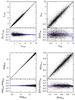 |
Fig. A.1 Comparison between Sérsic parameters of approximately 4000 simulated galaxies and their recovered values. Bottom plots show the fractional deviation of the parameters as a function of the half-light radius re in pixels, minor to major axis ratio b/a, and apparent magnitude m and Sérsic index n. The red line shows the median, whereas the blue line denotes the 1σ scatter around the median, defined to enclose 68% of the points at a given input value. |
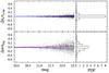 |
Fig. A.2 Distribution of the fractional deviation of the Sérsic index n and the effective radius re as a function of the apparent magnitude. The red lines shows the median, whereas the blue ones denote the 1σ scatter around the median. |
To assess the robustness of the presented galaxy profile fitting procedure we performed simulations similar to those presented in the literature (Häussler et al. 2007; Longhetti et al. 2007; Guo et al. 2009; Pannella et al. 2009; Mosleh et al. 2013). To estimate the accuracy of the results obtained from GALFIT, we applied exactly the same fitting procedure as that used for the real objects to a set of approximately 4000 (i.e. ~10% of a real sample) artificial galaxies.
Simulated objects were generated using the Sérsic parameters from the GALFIT output of the randomly selected VIPERS galaxies, with reduced value smaller than 1.2. This way gives more realistic parameter distributions of the galaxy population than randomly generated parameters and allows us to compare both results for each single object. GALFIT was used to create the artificial galaxies.
Each simulated profile was added to a different background image. To construct the background we applied a method similar to that proposed by Longhetti et al. (2007). The background image has been obtained by mosaicing different portions of the object-free regions of the CFHTLS tile into one large image. Then, the generated profile of each galaxy was superimposed on the randomly selected region of the background. The advantage of this method is that the background retains the same noise characteristic as the real CCD image. Finally the galaxy profile was convolved with the PSF of the i-band image generated at the galaxy position.
Simulated images of galaxies prepared in this way were analysed by SExtractor and GALFIT using the same procedure as that used for the real objects. The results of our tests are presented in Fig. A.1. The top plot of each panel shows the relationship between the input and output parameter values, whereas the bottom one presents the estimated uncertainty of the Sérsic profile parameters, that is, the half-light radius re in pixels, Sérsic index n, axis ratio b/a and apparent magnitude m. The red lines in the bottom figures show the median and the blue lines indicate the 1σ scatter around the median, defined as that which encloses 68% of the points.
Median fractional deviation of the half-light radius re, Sérsic index n, apparent magnitude m axis ratio b/a with the ±34% uncertainties about the median and in three magnitude bins from 19.5 to 22.5 mag.
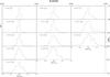 |
Fig. A.3 Distribution of the fractional deviation of the Sérsic index n as a function of redshift and luminosity. In each bin the histogram of the fractional difference Δn/ninp with their median and 1σ uncertainties around the median (i.e. the 16th and 84th percentile of values) are shown. |
The results of the tests presented in Fig. A.1 and Table A.1 demonstrate that the Sérsic function parameters are well recovered: the fractional derivative scatter around the median of galaxy apparent magnitude m is very small and only slightly increases for the less luminous galaxies. Similar results from GIM2D and GALFIT were obtained by Pannella et al. (2009). Simulations show that the error of the recovered value of the half-light radius re is larger for smaller galaxies. However, even in this case, the difference between input and output parameters presented in Fig. A.1 is less than 10%. The small systematic differences between those values was also reported in other studies (Häussler et al. 2007; Longhetti et al. 2007; Guo et al. 2009). Moreover, we found that the axis ratio b/a of the galaxy light profile is robust. The uncertainty of this parameter is in the order of a few percent.
The analysis shows that the Sérsic index n is also well recovered. However, in this case we observe a larger fractional deviation scatter around the median than for the two previously mentioned parameters. Figure A.1 shows that the fractional deviation of the Sérsic index n is almost uniformly distributed over the n. Similar scatter of the reconstructed parameters is also reported in other studies (Häussler et al. 2007; Longhetti et al. 2007; Guo et al. 2009).
The test shows that the error of the half-light radius re is larger for smaller galaxies and decreases with the object’s size. This effect is strongly correlated with the FWHM size of the PSF: for small re values, comparable with the FWHM, the image deconvolution becomes less accurate (e.g. Trujillo et al. 2001a).
The carried out simulations show good agreement between the input and output Sérsic function parameters. The 1σ deviation of values (i.e. containing 68% of points) about the parameter median is narrow, and, for the majority of the tested objects, the error of recovered parameters is less than 10%.
In the study of the distant galaxies, the typical size of a galaxy registered on the CCD images is small and can influence their estimated light profile parameters. We also verified the accuracy of the Sérsic index n and half-light radius re as a function of the apparent magnitude. The results are shown in Fig. A.2. As expected, this figure shows that faint galaxies exhibit larger random uncertainties in their Sérsic index Δn/ninp and half-light radius Δre/re,inp.
Figure A.2 shows that, in both cases, the error of recovered parameters is smaller for the brighter galaxies and, as expected, systematically increases for faint objects. For faint galaxies, the external part of the objects can fall under the sky surface brightness and this effect can lead to increases in the value of Sérsic index n. The test shows no systematic bias. The distribution of errors in the whole analysed luminosity range is symmetric.
The last test we present shows the fractional difference of the Sérsic index as a function of redshift and luminosity. To do this we applied the same binning as was used in our analysis and presented in Figs. 3, 5 and 7, to estimate the reliability of our study.
The simulated, approximately 4000 objects were generated using the Sérsic parameters from the GALFIT output as described in the first test. Galaxies were then divided into redshift-luminosity samples to compute the mean and standard deviation of the distributions of the fractional difference Δn/ninp.
Figure A.3 presents the results and shows histograms and median value with the ± 34% scatter around the median. The histograms show that the accuracy of the Sérsic index n estimation decreases with redshift but increases with luminosity. The most accurate value of n we get is for the nearby and most luminous galaxies. As expected, faint galaxies exhibit larger random uncertainties in their Sérsic index n parameter, consistent with the previous test. The histograms and numerical values presented in Fig. A.3 show no systematic deviation of the Sérsic index fitted to the galaxy images. The tests presented here show that Sérsic function parameters computed by GALFIT from CFHTLS CCD images of the VIPERS galaxies are robust.
Appendix B: Modelling of the PSF
The CFHTLS images were obtained with MegaCam at the prime-focus with wide-field corrector (Boulade et al. 2000). However, while the corrector is optimised to produce a uniformly high-quality image over the whole field of view, it also introduces large-scale non-linear geometrical distortions (Cuillandre et al. 1996). This effect, together with the seeing, significantly disturbs the isotropy of the PSF and has to be corrected before any further measurements are done from the images.
There are many methods of PSF construction. The atmospheric turbulent structure is well characterised by Kolmogorov statistics (Kolmogorov 1961; Goodman 1985). To reproduce the observed PSF, an additional distortion coming from the telescope optics needs to be modeled, by the sum of Gaussians or Gaussian-like functions, for example (e.g. Schechter et al. 1993; Hogg & Lang 2013), the Moffat (1969) function, their combination or the Gauss-Laguerre function as applied by Bertin in PSFEx from astromatic package2. It is expected that the high image resolution (FWHM< 0.1″) of space telescopes, free from the atmosphere influence, should allow for better modelling of the optics aberrations than ground-based ones. In this case the more precise PSF estimation, given by PSFEx, for example, is needed. In this study we used the Moffat function (Moffat 1969). It allows us to precisely reconstruct the anisotropy of the CFHT field of view as shown in the tests presented at the end of this section. The elliptical PSF for the CFHTLS images has been approximated by the Moffat (1969) function 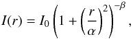 (B.1)where I0 is the central luminosity, β is the profile shape parameter and α is the half-light radius of the profile.
To construct a proper PSF for the VIPERS galaxies across the whole 1° × 1° CCD field we carefully selected stars from each CFHTLS tile. The stars were taken from the stellar branch of the SExtractor (Bertin & Arnouts 1996) MAG_AUTO versus FWHM_IMAGE diagram within the apparent magnitude range from 18 to 22 mag. Figure B.1 presents two examples of this diagram computed from images with good and bad quality. In the first plot, the vertical region dominated by the point-like objects is sharp, whereas in the second one it is significantly wider. To remove small and distorted stars, the objects with SExtractor ISOAREA_IMAGE ≤ 10 pixels and ELLIPTICITY > 0.2 were rejected from the analysis. Visual inspection of the CCD images confirmed that these criteria very accurately select isolated and non-distorted point-like objects.
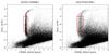 |
Fig. B.1 MAG_AUTO versus FWHM_IMAGE plot used to select PSF candidate objects for two CFHTLS tiles with good (left panel) and worse (right panel) image quality. The selected PSF candidate stars are enclosed in the red rectangles. |
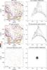 |
Fig. B.2 Whisker plot (left column) and the complex ellipticities (right column) obtained from the PSF parameters for the 022539-041200 tile in the i-band. The upper panels show the results obtained from uncorrected star ellipticities, the middle panels – from the 2D polynomial approximation of the Moffat parameters and the bottom panels – the final results after the correction for the anisotropy was applied. The small bar at the left-bottom corner of all left panels shows the ellipticity e = 0.1. Apparent i magnitudes are marked by colours given in the vertical colour bar: values of 18–19 mag by red, values of 19–20 mag by green, values of 20–21 mag by blue, and values of 21–22 mag by orange. |
The average number of stars used for the approximation of the Moffat parameters, and uniformly distributed in each 1° × 1° CFHTLS tile, is approximately 2000 and varies from field to field (between ~1000 and ~3500).
However, the applied method might be somewhat restrictive. Because of the image distortion presented in some CFHTLS tiles, there are regions where no PSF stars were selected by this algorithm, as shown in the top-left plot in Fig. B.2. This occurs mainly in the regions close to the tile border, covering approximately 2% of the total VIPERS area. Since the quality of the PSF plays such an important role in the GALFIT image deconvolution, we excluded galaxies from these regions from the presented analysis.
From the theoretical point of view, the shape of the PSF plays an important role in the inverse problem of image reconstruction, that is, estimation of the Sérsic function parameters (e.g. Trujillo et al. 2001a). At first, the FWHM of the modeled PSF should correctly reflect the light distribution in point-like objects. Due to optics aberrations, obstruction and mechanical problems the real PSF has wings which also need to be correctly modelled. However, when the PSF is regular, it has small wings and the FWHM of the PSF is correctly estimated, the requirement of the high quality PSF model is not crucial to obtain reasonably recovered galaxy structural parameters (e.g. Davari et al. 2014; Trujillo et al. 2001a).
In the following step, the Moffat function was fitted to the images of stars extracted from the CFHTLS tiles in the form of the postage stamps of size 35 × 35 pixels each, which is more than ten times larger than the FWHM. Then, for each CFHTLS tile of size of 1° × 1°, the fitted parameters of the Moffat function were approximated by the two-dimensional Chebyshev polynomial. The Chebyshev approximation was used due to its numerical stability and the smallest maximum deviation from the approximated function (Dahlquist & Bjorck 1974). We have checked polynomials of degrees from 5 to 11 and found that a polynominal degree of 7 best approximates the Moffat function parameters across the CFHTLS tile. In this way, we obtained an analytical form of how each of the Moffat function parameters varies across the whole field, which allowed us to compute the PSF at the position of every galaxy in the tile.
In the following two steps we verify the computed PSF approximation. We exclude stellar-like sources which show too much difference between the data and the model, and repeat the Moffat function fitting to the remaining stars, as shown above. Finally, we get the best description of the Moffat function in each CFHTLS tile point.
The first verification of our PSF modelling was performed using the whisker plot (Van Waerbeke et al. 2000; Tewes et al. 2012). This diagram demonstrates how the ellipticity e and the orientation θ of PSF stars vary across the field. Each selected star is represented by a line whose length represents the star ellipticity e, and is orientated to match the position angle of the star’s major axis. The colour of each line represents the i-band magnitude of the star. The first plot in the top row of Fig. B.2 shows a strong anisotropy of observed stars which should be corrected for. To do this, we applied the complex ellipticities (Tewes et al. 2012) defined by  (B.2)where the elongation is defined as ϵ = b/a. This representation is commonly used in anisotropy determination in gravitational lensing analysis (Holhjem et al. 2009; Van Waerbeke et al. 2000).
We performed a 3σ clipping procedure on the corrected stellar complex ellipticities e1 and e2 (Tewes et al. 2012), which removed most of the stars whose shape was deformed. After this procedure, for each tile, the parameters of the Moffat function were approximated again by the two-dimensional Chebyshev polynomial degree of 7. This iteration leads us to the final analytical approximation of the PSF coefficients used to reconstruct the PSF at the position of each VIPERS galaxy.
As an example of the method described above, Fig. B.2 presents the selected plots obtained from the final Moffat function parameters for the lower quality CFHTLS_022539-041200 tile in i-band. The diagrams in the second row of the figure were obtained from our global PSF approximation. The plots presented in the first and second rows show very good correlations between the observed and approximated results. The last row in Fig. B.2 shows the PSFs of stars after the correction for anisotropy. One can observe that the field corrected for telescope anisotropy is almost uniform, which confirms the high quality of our PSF approximation. Even for a tile with an image distortion as high as the one presented in this example, our method accurately maps the variation of the PSF across the whole field of view.
The tests presented above demonstrate that the anisotropy of images produced by wide-field cameras on modern telescopes can be large. Strong distortions introduced by the optics significantly change the ellipticity and orientation of the PSF. In the example presented in Fig. B.2 the PSF ellipticity varies from a value near 0 up to e ≈ 0.3 and there is a large range of PSF positional angle. When the FWHM size of the PSF is significantly smaller than the galaxy size, we can obtain accurately recovered galaxy morphological parameters (e.g. Davari et al. 2014; Trujillo et al. 2001a). However, if the FWHM and galaxy are comparable in size, the recovered parameters are biased due to the wrong PSF shape. Thus precise PSF modelling plays a vital role in the successful galaxy image decomposition by GALFIT.
All Tables
Median fractional deviation of the half-light radius re, Sérsic index n, apparent magnitude m axis ratio b/a with the ±34% uncertainties about the median and in three magnitude bins from 19.5 to 22.5 mag.
All Figures
|
Fig. 1 Distribution of ΔBev, as defined in Eq. (1), as a function of redshift z for galaxies in the VIPERS sample. The red lines enclose the selected sub-samples of galaxies. The right-side vertical axis shows the values of the absolute magnitude MB for a fixed redshift z = 0.7. |
| In the text | |
|
Fig. 2 Density of the VIPERS galaxies in the rest-frame (U−B) versus (B−V) colour–colour diagram. The contour lines show the galaxy density distribution in five equally spaced levels from 10% to 99% of the maximum value. The histogram shows the galaxy number density distribution projected along the line A−A connecting the two maxima of this distribution. The colours show the median sSFR 1/yr values of galaxies derived from SED fitting in seven equally spaced logarithmic bins. |
| In the text | |
|
Fig. 3 UBV rest-frame colour distributions (black histograms) of VIPERS galaxies in different redshift (increasing from left to right) and luminosity (from top to bottom) bins. The blue and red curves represent the Gaussian components fitting the colour distribution of the two galaxy populations, and the vertical dashed lines mark the maxima of the Gauss functions. The solid brown line shows the sum of the two Gaussians. The central values and 1σ widths of the Gaussians for the blue and red galaxy populations are labeled in each panel, in the top left and right respectively. The number of galaxies considered in each bin is also shown in the bottom right of each panel. |
| In the text | |
|
Fig. 4 Four examples of the GALFIT image approximation procedure. Left column: postage stamps with observed galaxies; middle column: best-fit PSF-convolved Sérsic model to each galaxy; right column: residual images. The small horizontal bars in the left column correspond to 1″. |
| In the text | |
|
Fig. 5 Sérsic index distribution (black histograms) for different redshift (from left to right) and ΔBev luminosity bins (from top to bottom). The blue and red solid lines show the Gaussian fits to the disc-like and spheroid-like populations, respectively. The vertical dashed lines mark the central values of each Gaussian. The sum of the two Gaussian fits is shown as a solid brown line. The central values ⟨ n ⟩ of the Gauss functions, their 1σ widths, and the total number of galaxies in each bin are shown in each panel. |
| In the text | |
|
Fig. 6 Sérsic index – redshift relation: VIPERS results are presented as red and blue solid lines for spheroid- and disc-like galaxies, respectively, for three values of B-band absolute magnitude. Patel et al. (2013)’s results for quiescent and star-forming objects with log (M/M⊙) > 10.5 are shown as red filled and empty circles and dashed magenta and blue lines. The relation found by van Dokkum et al. (2010) for a constant co-moving number density sample is plotted in brown (short-dashed line and triangles). Buitrago et al. (2013)’s results for a sample visually classified into early- and late-type galaxies is shown as orange filled and empty diamonds, while disc-galaxies measured by Tamm & Tenjes (2006) are represented by green squares. The dot-dashed lines show n(z) relation corresponding to the disk-like and spheroidal galaxies, only for MB = −21 mag, obtained from the 2D analysis presented in Sect. 6. |
| In the text | |
|
Fig. 7 UBV rest-frame colour vs. Sérsic index n distribution. Each panel shows the colour–coded galaxy surface density distribution map of the VIPERS galaxies in each redshift and ΔBev luminosity bin. The colour bar presented in the bottom right corner gives the normalised galaxy surface density. The contour lines show the density values in steps of 0.2 obtained from the two Gaussians bivariate fitting procedure. Blue and red dashed lines show the 2-dimensional model given by Eqs. (11)–(14). Crosses identify the positions of the centre maximal surface density distribution of the given galaxy population. The dashed lines around the peaks show the value of 0.5σ of the Gaussian fit. The histograms present the galaxy distributions projected on the Sérsic index and UBV colour axes, at the bin z = [0.65,0.80] and ΔBev = [0.5,0.0]. |
| In the text | |
|
Fig. 8 UBV rest-frame colour versus Sérsic index log (n) relation of late-type (lower left corner) and early-type (upper right corner) galaxies. Dots indicate redshift from z = 0.5 to 1.0 in increments of 0.1. Black solid lines connect the values of ΔBev from −1.5 to 1 in 0.5 magnitude increments. The arrows show the direction of the redshift and luminosity galaxy evolution. The right plot presents the UBV colour versus sSFR relation. The 0.2 dex background contour lines show the bivariate number density of all studied VIPERS galaxies in our sample (0.5 <z< 0.95). The yellow coloured regions mark the analysed redshift and luminosity limits, as presented in Figs. 1 and 7. |
| In the text | |
|
Fig. A.1 Comparison between Sérsic parameters of approximately 4000 simulated galaxies and their recovered values. Bottom plots show the fractional deviation of the parameters as a function of the half-light radius re in pixels, minor to major axis ratio b/a, and apparent magnitude m and Sérsic index n. The red line shows the median, whereas the blue line denotes the 1σ scatter around the median, defined to enclose 68% of the points at a given input value. |
| In the text | |
|
Fig. A.2 Distribution of the fractional deviation of the Sérsic index n and the effective radius re as a function of the apparent magnitude. The red lines shows the median, whereas the blue ones denote the 1σ scatter around the median. |
| In the text | |
|
Fig. A.3 Distribution of the fractional deviation of the Sérsic index n as a function of redshift and luminosity. In each bin the histogram of the fractional difference Δn/ninp with their median and 1σ uncertainties around the median (i.e. the 16th and 84th percentile of values) are shown. |
| In the text | |
|
Fig. B.1 MAG_AUTO versus FWHM_IMAGE plot used to select PSF candidate objects for two CFHTLS tiles with good (left panel) and worse (right panel) image quality. The selected PSF candidate stars are enclosed in the red rectangles. |
| In the text | |
|
Fig. B.2 Whisker plot (left column) and the complex ellipticities (right column) obtained from the PSF parameters for the 022539-041200 tile in the i-band. The upper panels show the results obtained from uncorrected star ellipticities, the middle panels – from the 2D polynomial approximation of the Moffat parameters and the bottom panels – the final results after the correction for the anisotropy was applied. The small bar at the left-bottom corner of all left panels shows the ellipticity e = 0.1. Apparent i magnitudes are marked by colours given in the vertical colour bar: values of 18–19 mag by red, values of 19–20 mag by green, values of 20–21 mag by blue, and values of 21–22 mag by orange. |
| In the text | |
Current usage metrics show cumulative count of Article Views (full-text article views including HTML views, PDF and ePub downloads, according to the available data) and Abstracts Views on Vision4Press platform.
Data correspond to usage on the plateform after 2015. The current usage metrics is available 48-96 hours after online publication and is updated daily on week days.
Initial download of the metrics may take a while.