| Issue |
A&A
Volume 597, January 2017
|
|
|---|---|---|
| Article Number | A114 | |
| Number of page(s) | 22 | |
| Section | Catalogs and data | |
| DOI | https://doi.org/10.1051/0004-6361/201629199 | |
| Published online | 12 January 2017 | |
Source clustering in the Hi-GAL survey determined using a minimum spanning tree method⋆,⋆⋆
1 Observatoire astronomique de Strasbourg, Université de Strasbourg, CNRS, UMR 7550, 11 rue de l’Université, 67000 Strasbourg, France
e-mail: This email address is being protected from spambots. You need JavaScript enabled to view it.
2 Instituto de Radio Astronomía Milimétrica, Avenida Divina Pastora, 7, Local 20, 18012 Granada, Spain
3 Astrophysics Research Institute, Liverpool John Moores University, IC2 Liverpool Science Park, 146 Brownlow Hill Liverpool L3 5RF, UK
4 INAF – Istituto di Astrofisica e Planetologia Spaziali, via Fosso del Cavaliere 100, 00133 Roma, Italy
Received: 27 June 2016
Accepted: 7 October 2016
Abstract
Aims. The aims are to investigate the clustering of the far-infrared sources from the Herschel infrared Galactic Plane Survey (Hi-GAL) in the Galactic longitude range of −71 to 67 deg. These clumps, and their spatial distribution, are an imprint of the original conditions within a molecular cloud. This will produce a catalogue of over-densities.
Methods. The minimum spanning tree (MST) method was used to identify the over-densities in two dimensions. The catalogue was further refined by folding in heliocentric distances, resulting in more reliable over-densities, which are cluster candidates.
Results. We found 1633 over-densities with more than ten members. Of these, 496 are defined as cluster candidates because of the reliability of the distances, with a further 1137 potential cluster candidates. The spatial distributions of the cluster candidates are different in the first and fourth quadrants, with all clusters following the spiral structure of the Milky Way. The cluster candidates are fractal. The clump mass functions of the clustered and isolated are statistically indistinguishable from each other and are consistent with Kroupa’s initial mass function.
Key words: stars: formation / stars: luminosity function, mass function / Galaxy: structure / infrared: stars / catalogs
Hi-GAL is a key-project of the Herschel Space Observatory survey (Pilbratt et al. 2010) and uses the PACS (Poglitsch et al. 2010) and SPIRE (Griffin et al. 2010) cameras in parallel mode.
The catalogues of cluster candidates and potential clusters are only available at the CDS via anonymous ftp to cdsarc.u-strasbg.fr (130.79.128.5) or via http://cdsarc.u-strasbg.fr/viz-bin/qcat?J/A+A/597/A114
© ESO, 2017
1. Introduction
In recent years, the development of Galactic Plane surveys has allowed for the statistical properties of the star-formation process to be examined because these surveys encompass many different Galactic environments. These environments cover all length scales, from kpc, which allows studying interactions in the spiral arms, to pc scales, which enable us to study individual star-forming regions. Studies have started to show that, on large scales, there are no major variations in the star-formation efficiency caused by the spiral arms (Moore et al. 2012; Eden et al. 2013, 2015) but that the sub-10-pc scales may be the most important, with the most significant variations found on these smaller scales (Eden et al. 2012; Vutisalchavakul et al. 2014). These results point towards the smaller scales as the most important, and therefore local triggering may be vital in the star-formation process (e.g. Deharveng et al. 2005; Thompson et al. 2012; Kendrew et al. 2012).
Billot et al. (2011) used the Herschel infrared Galactic Plane Survey (Hi-GAL; Molinari et al. 2010b, 2016) science demonstration phase (SDP) fields to study the clustering of star-forming clumps, within two 2 × 2 square deg fields. In this paper, we extend this to cover ~1/3 of the Galactic Plane, in the Galactic longitude range of −71 deg to 67 deg, spanning the first and fourth quadrants (Molinari et al. 2016).
We use the minimum spanning tree (MST) method to investigate the clustering of star-forming clumps traced at far-IR-submm wavelengths. Single-band catalogues at 70, 160, 250, 350, and 500 have been merged together (Elia et al. 2016) to produce a band-merged catalogue that is the starting point of our cluster analysis. A byproduct of identifying the clumps that fall into these clusters is that field clumps will also be identified, allowing for a comparison between these two environments. Measurements of the stellar initial mass function (IMF) in the Galaxy and in extragalactic structures find that the IMF is invariant, with no significant differences found (Bastian et al. 2010). Observers have found (e.g. Beltrán et al. 2006; Simpson et al. 2008) that the clump mass function (CMF) shape matches the IMF either as slope or turnover mass once a constant mass offset is applied. With this observational evidence, any changes detected in the CMFs of different environments may therefore indicate a change in the IMF.
The band-merged Hi-GAL product catalogue (Elia et al. 2016) is built as in Elia et al. (2013) and provides spectral energy distribution (SED) fit parameters to the individual clumps. The average angular size of the clumps is 25′′ at 250 μm. Using the heliocentric distances provided in the Hi-GAL product catalogue (described in Sect. 3.2.) and the SED fit parameters, the authors of the catalogue are able to provide linear diameters and masses of the clumps. The catalogue explores a wide range of linear diameters and masses, from sub-parsec (≤ 0.1 pc) to parsec scale (1−5 pc) with masses from 1 M⊙ to 105M⊙. These wide ranges mean that we probably mix several types of objects, from single star-forming cores to clumps containing multiple cores, even to entire clouds, depending on the distance of object. Most of these sources, however, fulfil the definition of clump, according to the definition of Bergin & Tafalla (2007). Dust temperatures for these clumps have been estimated through a grey-body fit, and searched in the range T = 5−40 K. Most of them are found between 10 and 20 K. The appearance of the SED and the parameters obtained through the grey-body fit allow for classifying the evolutionary stage of these objects. Three stages are identified: starless unbound and bound (pre-stellar) objects, and proto-stellar objects. The pre- and proto-stellar stages are distinguished from each other by the presence of a 70 μm source in a proto-stellar clump (e.g. Dunham et al. 2008; Ragan et al. 2012; Veneziani et al. 2013). The bound versus unbound identification is obtained by using the mass-radius relation, well known as Larson’s third law, originally formulated as M(r) > 460 M⊙(r/ pc)1.9, with r the radius of the source (Larson 1981). Beyond 4−5 kpc two effects could lead to misclassifying the pre- and proto-stellar stages. First, different sensitivities of PACS and SPIRE could lead to missing a possible 70 μm counterpart of a source detected with SPIRE. Second, at large heliocentric distances, two or more pre- and proto-stellar sources could be detected as a single object as a result of lacking resolution, globally and simply labelled as proto-stellar. The first effect was partially mitigated by searching for a possible 70 μm counterpart that was not originally listed in the single-band catalogue through performing additional source detection at this band using a threshold less demanding than the initial one. Elia et al. (2016) provide statistics and a discussion about the ratio between pre- and proto-stellar clumps. The distribution of the three evolutionary stages is shown in a portion of the Galactic Plane in Fig. 1. Each panel represents an evolutionary stage in the longitude range 26 ≤l≤ 31 deg. The pre-stellar clumps are more extended in Galactic latitude than the proto-stellar clumps. The unbound clump distribution is hard to characterise because it is obscured by the proto-stellar clumps in the mid-plane, therefore we only consider clustered over-densities composed of pre- and proto-stellar clumps. These distributions are observed across the entire longitude range of this study.
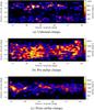 |
Fig. 1 Source density maps of a sub-sample of the three different types of clumps defined in the Hi-GAL product catalogue, located in the longitude range 26 ≤l≤ 31 deg. The same distributions are observed for the whole sample. |
Additional evolutionary markers, such as H ii regions, a marker of high-mass star formation (Urquhart et al. 2013) and infrared dark clouds (IRDC), can be associated with the clustered clumps, giving further insight into the environmental conditions.
This paper is arranged as follows. Section 2 introduces the MST method, allowing the clustered clumps to be identified, with Sect. 3 describing the process of applying the method to the Hi-GAL data. In Sect. 4 we present the results of the study, with Sect. 5 comprising the discussion, whilst Sect. 6 presents the catalogue of over-densities. Finally, Sect. 7 contains the summary and conclusions.
2. Minimum spanning tree method
Clumps in these wavelengths are mostly associated with filaments (e.g. Molinari et al. 2010a). For this reason, we decided to use an MST method, which is well suited to find sources along filamentary structures. This method was first described in Borůvka (1926a,b), with an English translation provided in Nešetřil & Nešetřilová (2012). Since this time, several algorithms have been described, with Graham & Hell (1985) providing a detailed historical evolution of the MST algorithm. For this study we used Prim’s algorithm (Prim 1957). More details about Prim’s algorithm can be found in Schmeja (2011).
The MST method belong to undirected graph theory. Using Delaunay triangulation (e.g. Shamos & Hoey 1975; Toussaint 1980), the method connects all points, called vertices, with branches, or edges, without creating closed loops whilst minimising the total length of the branches. As all lengths are different, the solution of the MST analysis is unique. In this case, the vertices correspond to the clumps, and the edges, Λ, correspond to the angular distance separating the clumps regarding the solution found with the MST method. This algorithm was originally used in an astrophysical context for galaxy clusters. More recently, it was used in stellar clusters, for instance in Koenig et al. (2008), Gutermuth et al. (2009), Billot et al. (2011) and Saral et al. (2015). This method was also recently used to observe the mass segregation into star clusters in Allison et al. (2009), Maschberger & Clarke (2011), and Parker et al. (2012).
For this study we followed the recommendations of Koenig et al. (2008) and Gutermuth et al. (2009) to analyse the trees that are determined. By producing the cumulative distribution of the branch lengths, an estimate of the branch cut-off length, Λcut, can be found. Two segments are fitted to each extreme of the cumulative distribution with the first to the small branches, whereas the other one will fit the large branches. The intersection of these two segments provides a branch cut-off length Λcut. Differently from other methods where the cut-off threshold is chosen manually, this method allows an automatic setting of the cut-off.
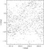 |
Fig. 2 Distribution of pre-stellar and proto-stellar clumps in a 2 × 2 square deg field centred on l = 330 deg. |
Figure 2 shows the distribution of Hi-GAL proto-stellar and pre-stellar clumps for a 2 × 2 deg2 region of the sky centred on l = 330 deg. From this sub-sample, we can determine the branch cut-off length by using the branch distribution as shown in Fig. 3. Figure 3 shows the cumulative distribution (in black) from the histogram of branches (in grey) of this sub-sample. The intersection of the two linear fits corresponds to a Λcut of 160′′ for this sub-sample. Only branches smaller than Λcut are considered. The result for this field is presented in Fig. 4. Over-densities are represented by their convex hulls. Some hulls seem to overlap others, but this appears to be a problem of representation of the correct shape for the over-densities. Some points that should belong to a convex hull are ignored and a straight line is drawn instead of several segments. A clump belongs to only one over-density and always respects the criterion of the cut-off branch length. Following the recommendation of Gutermuth et al. (2009), we applied a threshold of the minimum number of clumps required to form an over-density, using a threshold of N = 10 clumps. Most of the visual over-densities in Fig. 2 can clearly be found by the MST method.
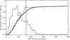 |
Fig. 3 Distribution of the branch lengths found in the field displayed in Fig. 2. The grey line corresponds to the branch length histogram, whilst the black line is the cumulative distribution. The two dashed black lines are the fitted segments to the cumulative distribution. The dashed-dot line shows the cut-off branch length found at the intersection of these fits. |
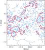 |
Fig. 4 Result of the MST method applied on the field in Fig. 2. Grey points and lines correspond to Λ > Λcut, whereas blue points and lines correspond to Λ < Λcut. Red lines correspond to convex hulls surrounding groups with N ≥ 10. |
3. Cluster catalogue definition
In this section we describe how we applied the method defined in Sect. 2 to the Hi-GAL catalogue. The whole catalogue is analysed in pieces within a rectangular window. The choice of the window affects the results in terms of cut-off threshold and number of clusters. The heliocentric distance estimates help us to distinguish probable clusters from the list of over-densities.
3.1. Effect of window size
The determination of Λcut is associated with the mean density of the sample. Higher mean densities result in lower values of Λcut. Figure 5 shows the Λcut distribution along the mean density. Each point corresponds to a solution of the MST for different fields and different ranges of longitude. The correlation between Λcut and the mean source density is well represented by a power law,  with a slope β ≈ 0.24 ± 0.01. The spread in the distribution highlights a strength of the MST method. The MST method can find over-densities even against a very busy background distribution, therefore the detection of over-densities depends on the density contrast between the over-densities and the background, as was reported by Schmeja (2011).
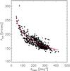 |
Fig. 5 Relation between Λcut and the mean density of the field considered. The red line corresponds to the correlation function |

The source density varies across the Galactic Plane, mainly as a result of Galactic structure features such as the Galactic Centre and the spiral arms, which will increase the number of sources. These variations are not seen dramatically in the latitude direction. The latitude range (2 deg) is smaller than the longitude range, with no large spatial variations due to Galactic structure.
This density variation along the longitude forced us to split the whole catalogue into rectangular windows. By not analysing the whole Galactic Plane together, fields need to be overlapped to avoid rejecting clumps that lie at the edges of fields. To avoid this, a new window was created by shifting a field in Galactic longitude by half. For each window, a branch histogram was built that determined a Λcut value. However, this potentially resulted in two values of Λcut and two different shapes for the over-density. As a result, the window in which the over-density was completely contained dictated the choice.
Figure 6 illustrates the process of rebuilding the whole catalogue. The top panel contains the overlap window, whilst the middle panel contains the two original windows. The lower panel houses the final catalogue for this Galactic longitude range. The grey shapes correspond to the convex hulls of the over-densities found in each window with at least ten members. The red shapes correspond to the convex hulls for the over-densities split into two by the original windows. The boxes correspond to the limits of the areas considered in the catalogue-building process.
As a result of the overlap, the choice of window size may have a strong effect on the result. The window size also needs to correspond to the spatial distribution of the data. To do this, a range of 2 to 30 deg was investigated, stepping along the data by a step of one window in size. The minimum size of 2 deg was chosen as this is the size of the Hi-GAL observation fields. This size also allows for a varied distribution in branch sizes, and is larger than the typical size of an over-density as displayed in Fig. 3. Therefore, the window size of 2 deg is large enough to conserve most branch lengths. The maximum value of 30 deg was chosen to be larger than tangents of spiral arms and the Galactic Centre.
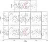 |
Fig. 6 Example of the reconstructing of the over-density catalogue found by the MST method at the split between windows. This example field is 10 deg large. Grey points are the pre-stellar and proto-stellar clumps. The grey shapes correspond to the convex hulls of the over-densities with at least ten members. The red shapes are the convex hulls of the over-densities split over the two original windows. The black dashed and solid lines mark the separation limits for each window. The top window is the overlap window. The middle windows are the two original windows of this field. The bottom window is the result of the overlapping method. |
Furthermore, we evaluated the non-random clustering of sources, that is, whether the over-densities are real. Using the approach of Campana et al. (2008), the total length of an MST analysis, Λ, is proportional to  , where A is the window area and Ntot is the total number of clumps inside this window, and the mean length is proportional to
  . For a random-field MST analysis, Campana and collaborators found coefficients of ≈ 0.65 for both quantities from Monte Carlo simulations. We find mean coefficients of ≈ 0.51 ± 0.01 and ≈ 0.40 ± 0.01 for the total length and mean length, respectively, over all window sizes checked in this study. These values are significantly lower than what would be expected for a random-MST field, which means that the sources are distributed non-randomly. This result allows all window sizes to be considered.
Figure 7 shows a test of the effect of the window size as a function of Galactic longitude. By building 29 catalogues, one for each window size between 2 and 30 deg, and computing the fraction of clumps in over-densities, we plotted the mean of the 29 catalogues of this fraction in 5-deg bins. The error bars correspond to a 1σ error of the standard deviation in each bin, with the dashed and dot-dashed lines representing a variation of ±5% of the branch cut-off length, which is approximately 10′′ and represents a variation of 10−15% of the amount of clustered sources. This distribution shows that there is not much variation, other than at the edges of the longitude range, therefore the window size does not cause too much variation.
As the clustering fraction does not vary over the whole study region, we need to look at particular regions and study the effect of window size on these smaller regions. Again, only over-densities with over ten members were considered. Figures 8a and b show two particular regions with a size of 2 × 2 deg, centred on 335 deg (Fig. 8a) and 20 deg (Fig. 8b). The distribution of the clumps is different in the two regions, with the field centred on 335 deg having a higher source density than at 20 deg. In both distributions, one window size does not vary the fraction of clustered clumps, but in the higher density 335 deg window, using a window larger than ~20 deg causes a greater jump in the fraction found. This fraction of clustered clumps is influenced by the cut-off threshold and by both the number and distribution of sources that lie within the window size.
It is also pertinent to try to remove small-scale variations, that is, those below 2 deg. Figure 9 shows the variation of Λcut along the Galactic longitude for four different window sizes, 2, 10, 20, and 30 deg. A larger window produces a smoother distribution of Λcut, with windows larger than 20 deg smoothing out any variation in source densities caused by Galactic structure. Comparing the results from Figs. 8a, b, and 9, the best range of window sizes appears to be 10−15 deg, with 10 deg chosen for this study. As a result, a catalogue of 1705 over-densities with at least ten members was found, which corresponds to 45 323 clustered clumps.
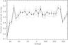 |
Fig. 7 Spatial distribution of the fraction of clustered clumps as a function of Galactic longitude. The black line corresponds to the mean fraction of clustered clumps of each master catalogue (one for each window size) for each 5 deg bin. The black points correspond to this mean and are located at the average longitude of each bin. The 1σ error bars correspond to the standard deviation of the fraction of clustered clumps for each bin. The grey dashed and dot-dashed lines correspond to a value of ±5% of Λcut. |
3.2. Heliocentric distance estimates
The 1705 over-densities characterised are distributions of clumps in two dimensions. As the Galaxy is three-dimensional, we wish to remove the casual clustering induced by projection along the line of sight. This selection in the catalogue cluster candidates can be made by using heliocentric distance estimates (named HDEs in the following) from the Hi-GAL product catalogue (Elia et al. 2016). These HDEs were extracted from the 12CO or 13C spectrum for each clump. The authors used data from the Five College Radio Astronomy Observatory (FCRAO) Galactic Ring Survey (GRS, Jackson et al. 2006) and the Exeter-FCRAO Survey (Brunt et al., in prep.; Mottram et al., in prep.) for the first quadrant. The NANTEN 12CO data were used for the fourth quadrant. When needed, the distance ambiguity was resolved by using the extinction maps and a catalogue of sources with known distances (H ii regions, for example). A case study calculating kinematic distances in the Hi-GAL SDP fields can be found in Russeil et al. (2011). Of the 99 083 Hi-GAL sources that cover all evolutionary phases, 57% have HDEs. Of the population of proto-stellar clumps, 64% have distance estimates. HDEs have not been obtained for sources in the longitude range −10 to +14 deg where kinematic distances cannot be estimated. When this range is discounted, 80% of the proto-stellar clumps have HDEs.
It is not suitable to use the distances to compute the MST analysis in three dimensions as the uncertainties on HDEs are very large (≈0.6 kpc and ≈0.9 kpc for the SDP l = 30 deg and l = 59 deg; Russeil et al. 2011) as Billot et al. (2011) discuss. This would result in rejecting large parts of the catalogue.
As a result, the MST was computed and the HDEs were used as a third dimension to evaluate the compactness of each over-density. For each over-density we computed the HDE histogram and assumed all the sources to belong to the cluster that lay within 1 kpc from its peak (Russeil et al. 2011). This range is called reliable distance, RD, in the following.
Two metrics were used to define the compactness. The first is the ratio of the number of sources inside the RD to the total number of sources with HDEs. The second is the ratio of the number of sources with HDEs to the total number of sources. A threshold of 70% of clumps inside the RD and 40% of clumps with HDEs was used for the two metrics. One last measure was used: each over-density must have five clumps with HDEs. Six hundred and seven over-densities satisfy the compactness criteria and have five clumps with HDEs, compared to the 1705 over-densities found in two dimensions.
Only 219 (36%) of the 607 over-densities have all clumps inside the RD. As a result, it was decided to remove the clumps that do not seem to belong to these cluster candidates. This would allow a test of the MST method, to determine whether it is able to reproduce the same cluster candidates.
A total of 1531 clumps were removed, with the MST analysis recomputed with the remaining 80 128 clumps. A total of 1633 over-densities were found, 449 of them having no clumps with HDEs. Of the remaining 1184 over-densities, 496 satisfy the thresholds of 70% of clumps inside the RD and 40% of clumps with HDEs. Forty of the remaining 1184 clumps have clumps outside of the RD. Of the final 496 over-densities, 364 have between 10 and 20 clumps (~70%), with 4 over-densities having at least 70 members. The final 496 candidates are composed of 9608 clumps, approximately 12% of the total 80 128 clumps, with 8248 (~86%) having HDEs.
The new MST analysis can still be considered a non-random distribution as a value of 0.36 ± 0.01 was found for the mean MST length and , which is still below the upper limit of 0.65 found by Campana et al. (2008).
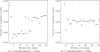 |
Fig. 8 Variation of the fraction of clustered clumps into 2 × 2 square deg fields for all window sizes between 2 and 30 deg. |
4. Description of the catalogues
As a result of the work in Sect. 3.2, two catalogues of over-densities, or cluster candidates, were created. The first is of the 496 cluster candidates, with part of this catalogue displayed in Table B.1. The sources in this catalogue are the most reliable detections and are used from here on to derive properties for the analyses in Sects. 5 and 6. The other is the potential cluster catalogue, consisting of the 1137 clusters rejected in the previous section. A part of this catalogue is displayed in Table B.2.
5. Results
5.1. Spatial distribution and cluster characterisation
5.1.1. Cluster candidate spatial distribution
The sources in this study are distributed between the first and fourth Galactic quadrants, with ~35%, 176 of the 496, found in the first quadrant. We split the two quadrants into two segments after visually inspecting the peaks in the longitude distribution of the cluster candidates, as displayed in Fig. 10. The segments are [15, 40] and [40, 60], and [320, 345] and [300, 320] for the first and fourth quadrants, respectively. We found 97, 72, 151, and 101 cluster quadrants in each of these segments, respectively. By using the HDEs, a 3D map can be produced, as displayed in Fig. 11. The cluster candidates trace the spiral arms well, with the spiral arms from the study of Englmaier et al. (2011) using the Galactic distribution of molecular gas. The good agreement with the molecular-gas traced spiral arms is achieved because the clumps are very young and have not had time to migrate from the molecular clouds from which they formed. Unsurprisingly, a majority of sources are found associated with the tangents of spiral arms, with peaks in Fig. 10 in the fourth quadrant corresponding to the tangent at l = 315. Other tangents, at l = 30 and l = 295, are washed out of the sample, either by the number of cluster candidates at distances closer to the Sun or by the edge of the studied region, respectively.
We also analysed the scale height, Z, of the cluster candidates from the Galactic Plane using the expression  (1)where Dpeak is the heliocentric distance of the cluster candidates. The HDE we used is the peak value of the cluster distance histogram. The Galactic latitude represents the central position of the cluster candidate. We also calculated the Galactocentric radius of each source using the relation
  (2)where R0 represents the Galactocentric distance of the Sun, set at 8.5 kpc. By calculating the mean scale height in Galactocentric radius bins of 0.1 kpc, we computed the profile of Zmean over the first and fourth quadrants; this is displayed in Fig. 12. We show in the lower panel of Fig. 12 the standard deviation, σZ, in each bin along R. We compared the Zmean profile to that of Paladini et al. (2004), who observed the distribution of H ii regions in the entire Galactic Plane. The profile in this study matches that of Paladini et al. (2004) in the fourth quadrant, with a break at ~7 kpc. The first quadrant shows a decrease in Zmean until ~6 kpc, at which an increase is observed (also observed by Paladini et al. 2004) until another decrease at 8.5 kpc. However, the range of R in the first quadrant is much shorter than that of the fourth, with no access to the sources at R greater than 10 kpc, where Paladini et al. (2004) observed an increase. The difference between the two quadrants at Galactocentric radii greater than 7 kpc is most likely due to the warp of the Galactic Plane (see Burton & Hartmann 1988). The warp is observed in H i (Henderson et al. 1982) as well as molecular clouds, OB stars, and the stars traced by 2MASS. An exhaustive list of the main components of the warp can be found in Reylé et al. (2008). The warp mostly occurs at Galactocentric radii larger than the solar circle. The cluster candidates lie in a thin, asymmetric disk in a range of Z from −248 to 134 pc. The asymmetry is due to the location of the Sun above the Galactic Plane (e.g. Brand & Blitz 1993; Reed 1997, 2006), as this would have more effect on the nearby sources. The mean value of Z in the entire study is −6.2 pc, again because of the position of the Sun.
Our data suggest the presence of the Galactic warp, but its amplitude is quite ambiguous. Similar results are also found in the star distribution, where the warp is hardly recognizable (Marshall et al. 2006; Reylé et al. 2008) with respect to the gas distribution. The study by Paladini et al. (2004) shows a flare at the scale height after 10 kpc, which cannot be observed here as shown with σZ in the lower panel of Fig. 12. However, our data do not exclude the flaring in the outer disk that is generally traced by the star distribution (Derriere & Robin 2001).
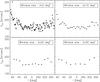 |
Fig. 9 Changes in the Λcut as a function of Galactic longitude in four different window sizes, with sizes of 2, 10, 20, and 30 deg. The Galactic longitude corresponds to the centre of each window. |
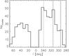 |
Fig. 10 Longitude distribution of the 496 cluster candidates. The visible tangents of the spiral arms are located at l = 315 deg (black dashed line). The tangent at l = 295 deg is marked by a grey line. |
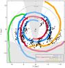 |
Fig. 11 Top-down view of the Galaxy using the HDEs of the cluster candidates. The spiral arm model is supplied by Englmaier et al. (2011), with the different colour lines marking their locations. The plus (+) symbol represents the position of the Sun, with the grey dashed lines corresponding to Galactocentric distances. The black dots mark the location of the cluster candidates. The two grey shaded regions represent the regions where no cluster candidates could be found. |
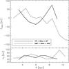 |
Fig. 12 Top: distribution of the mean scale height, Zmean, of cluster candidates as a function of Galactocentric radius. The black line corresponds to the cluster candidates in the first quadrant with the grey dashed line corresponding to the fourth quadrant. Bottom: distribution of the standard deviation, σZ, as a function of Galactocentric radius, R. |
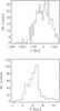 |
Fig. 13 Top: histogram of scale heights of the cluster candidates. The mean value is −6.2 pc. Bottom: distribution of cluster candidate Galactocentric radii. The peak is at ~6.5 kpc, a value also observed by Paladini et al. (2004). |
5.1.2. Spatial distribution of clumps in clusters
We used the parameter Q introduced by Cartwright & Whitworth (2004) to distinguish between centrally concentrated cluster candidates and those with a fractal distribution. The parameter is defined as  (3)where
  is the normalised mean branch length of the sub-tree of the cluster candidates, calculated from (NclumpsA)0.5/ (Nclumps−1), where Nclumps is the total number of clumps inside each cluster candidate and A is the area of the cluster.
  is the mean distance between clumps divided by the cluster candidate radius. Using simulated clusters, Cartwright & Whitworth (2004) identified fractal clusters as having a Q parameter value ≤ 0.8, whereas Q> 0.8 corresponds to concentrated clusters. Clusters with Q = 0.8 correspond to clumps with a random distribution, that is, unclustered clumps. Subsequent work of Cartwright (2009) found that clusters in the range 0.75 ≤ Q ≤ 0.85 could also follow a concentrated or fractal distribution. We found a range from Q = 0.4 to Q = 0.84 with 98.6% of cluster candidates below Q = 0.8 and 90% below Q = 0.75. This means that the cluster candidates follow a fractal distribution, as defined by the Q parameter of Cartwright & Whitworth (2004), as does the ISM (Combes 2000). This range is similar to one found by Parker & Dale (2015) in hydrodynamical simulations.
Cartwright & Whitworth (2009) found that the elongation of the cluster, the ratio between the semi-major and minor axes, could affect the value of Q for elongations above 3. Here only 40 cluster candidates have an elongation above this value, and no correlation between the two were found, therefore we decided against a correction to Q. The elongation could represent a filamentary distribution, therefore some cluster candidates with Q = 0.8 do not necessarily mean a random spatial distribution. Furthermore, Cartwright & Whitworth (2004) studied star clusters that may have a different distribution and may not present filamentary structures compared to the young sources investigated here. Other effects, typically observational limitations and statistical biases, can affect the Q parameter as developed in Bastian et al. (2009). The cluster candidates suffer from a lack of statistics because of the low number of clumps (88% of cluster candidates have ≤ 30 clumps) compared to the star clusters of Cartwright & Whitworth (2004) (≥ 100). This could affect the profile estimation of the cluster candidates. For example, a cluster with a random distribution but with a low statistic can have a fractal profile. By restraining the number of cluster candidates to those with the greater number of clumps (≥ 30 clumps), we observe that the values of the Q parameter remain in the same range, with a range from Q = 0.40 to Q = 0.77.
Two more metrics can be used to determine whether the cluster candidates are significant, or in other words, that their shapes are not random. The first of these is that of Campana et al. (2008),  (4)where
  is the mean branch length and
  is the mean branch length of the kth cluster. We find a range of gk from 0.95 to 3.02 with a peak at 1.5. The second metric is that of Massaro et al. (2009), which uses the relation between the number of clumps inside each cluster and gk,
 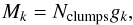 (5)where Nclumps is the total number of clumps in the kth cluster. This metric, called magnitude, allows us to compare clusters with all ranges of numbers of clumps. Mk has values from 9.5 to 380 and 54% of cluster candidates have Mk> 20. The peak of this distribution for our cluster candidates, which is 15, corresponds to a value of gk = 1.5 with Nclumps = 10. The two metrics give results indistinguishable from each other and are consistent with the studies that reported the definitions in the first place.
5.2. Clump mass functions
We compared the masses of clumps found in the 496 cluster candidates to those that are considered isolated. Any clump that is connected only by branch lengths greater than the cut-off branch length was considered to be isolated. This gives a total of 4752 isolated clumps compared to 8248 clustered clumps. The masses are computed with  (6)with the masses normalized with the quantity
  by taking the ratio of the peak distance in the cluster distance histogram compared to the individual source distance.
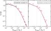 |
Fig. 14 CMFs of clustered (left panel) and isolated (right panel) clumps. The masses of the clumps are computed using Eq. (6) and the ratio |
CMF fitting results for clustered and isolated clumps in the whole sample, first and fourth quadrants.
These masses allow for the clump mass function (CMF) for the clustered and isolated clumps to be compared. The relation outlined in Eq. (7) was assumed (Kroupa et al. 1993). α is linked to the Salpeter slope (Salpeter 1955) by the relation α = Γ + 1,  (7)The bin size used in this study does not significantly alter the values of α as the number of clumps used is N> 500 (Rosolowsky 2005). A logarithmic bin of mass 0.1 was used for all CMFs, corresponding to the criterion of
 ![Mathematical equation: \hbox{${W} = 2(IQR)/\sqrt[3]{N,}$}](/articles/aa/full_html/2017/01/aa29199-16/aa29199-16-eq91.png) where W is the bin width, IQR is the interquartile range, and N is the number of sources in the whole CMF (Freedman & Diaconis 2011).
where W is the bin width, IQR is the interquartile range, and N is the number of sources in the whole CMF (Freedman & Diaconis 2011).
Figure 14 shows the CMFs for clustered (left panel) and isolated (right panel) clumps. The error bars correspond to the 1σ Poisson errors,  . The errors on the individual clump masses are not considered because the main error source is the distance uncertainty. A three-segment power law was fit to each CMF, with the form of Eq. (7). These three segments were compared with those of Kroupa’s IMF (Kroupa 2001, 2002). The lower bound is assumed constant in the analysis and equal to 10 M⊙. The fits provide values for the three quantities α1, α2, and α3, as well as the mass breaks, M1 and M2. Table 1 displays the fitting results for clustered and isolated clumps. These slopes are consistent both with each other and with the Kroupa IMF. The sample was also split into the two quadrants, and the clustered and isolated CMFs were reproduced. The results are also consistent with the Kroupa IMF. Table 1 also contains the fitting results for these CMFs. The figures of the first and fourth quadrant CMFs can be found in Appendix A (Figs. A.2 and A.3).
In all cases the break masses M1 and M2 are much greater in clustered than in isolated clumps.
A correlation is found between the highest mass clump in each cluster candidate and the total cluster mass, as shown in Fig. 15. The dashed line corresponds to the upper limit of the maximum mass, that is, the cluster mass. The red line is the linear fit to the distribution,  with ζ = 0.27 ± 0.04 and η = 0.98 ± 0.02. This correlation remains the same when the sample is split into heliocentric distance bins. Kirk & Myers (2012) and Weidner et al. (2010) observed the same correlation for YSO groups, but with a flatter slope of η ≈ 0.5. This suggests that different mechanisms act at these scales in producing and fragmenting the clumps.
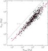 |
Fig. 15 Highest mass clump in each cluster candidate as a function of total cluster mass. The grey dashed line is the 1:1 line and a highest value for the highest mass clump. The red line is the linear fit to the distribution. |
6. Discussion
6.1. Completeness of the cluster candidate catalogue
The MST is a powerful method for finding over-densities in images, especially when over-densities are composed of filamentary structures. The branch-length cut-off, Λcut, can be determined by different methods. Here, the method described in Koenig et al. (2008) and Gutermuth et al. (2009) was used. Other methods include that of Battinelli (1991), who defined Λcut as the branch length that corresponds to the maximum number of over-densities in a sample. Maschberger et al. (2010) chose the branch length cut-off such that the properties of over-densities found correspond to the ones selected by eye.
The drastic drop in the number of over-densities (1633) found compared to cluster candidates (496) gives an idea of the line-of-sight projection effect that is stronger in the inner Galaxy. When the accuracy of the heliocentric distance estimates also improves, the number of cluster candidates increases and may allow for MST to be computed in 3D. The heliocentric distances are also a great source of uncertainty in the computation of clump mass that may affect the slopes of the CMF. A greater number of heliocentric distances will also increase the source numbers and reduce the Poisson errors in the CMF slope computations, which are the largest source of uncertainty in that analysis.
The fractal distinction of the cluster candidates implies that the clumps are gravitationally bound to their host cluster, but also that a non-random sub-clustering distribution can be observed. This means that sources are probably more spaced than in the case of a centrally concentrated cluster. We can investigate the physical distance between clumps and a possible bias by comparing our results with the typical Jeans length of clumps (Eq. (8)), which characterises the ability of a sphere to collapse, as well as with the resolution at the extreme wavelengths 70 μm and 500 μm,  (8)where kB is the Boltzmann constant, T is the temperature of the cloud, n is the mean volume density of the cloud, mp is the proton mass, and μ is the mean molecular weight. We considered temperatures of 10, 20, and 30 K with a mean volume density of 105 particles per cm3 and an average mass per particle μmp = 4 × 10-27 kg, assuming a cloud composed of 80% hydrogen and 20% helium and μ ≈ 2.5. These values give a Jeans length of 0.05 pc to 0.1 pc. This length would be larger if we considered a cloud with magnetic fields and under external pressure. Figure 16 shows the relation of projected distances (in pc) computed from the MST branches Λ characterising the angular distances between clustered clumps, with the HDE of the clumps taken equal to the mean distance of the cluster candidates. The lowest value, ≈ 0.13 pc, is comparable to the highest value of the Jeans length. Distances computed in three dimensions are greater than the projected distances and increase the difference with the Jeans length. We also plot the linear diameter of the beam at 70 μm (in green) and 500 μm (in orange) in the heliocentric distance range that covers our sample as well as the highest value of the Jeans length (0.1 pc, in grey). All physical distances between clumps are greater than the 70 μm beam size and more than 90% are greater than the 500 μm beam size. This means that the clumps are separated by much more than the imprints that each of them leaves on the fragmented cloud. The PACS and SPIRE resolutions introduce a bias by not allowing us to detect clumps with a spacing shorter than the Jeans length, as has been mentioned in Billot et al. (2011).
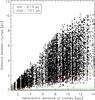 |
Fig. 16 Distribution of the distance between clustered clumps in cluster candidates. The green dashed line represents the linear diameter of the beam at 70 μm. The orange dashed line corresponds to the same size, but at 500 μm. The grey line marks the Jeans length (0.1 pc). |
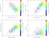 |
Fig. 17 Cluster candidate properties as a function of mean clump mass. Top left: cluster density versus mean clump mass. Top right: mean MST clump length versus mean clump mass. Bottom left: cluster area versus mean clump mass. Bottom right: number of clumps versus mean clump mass. The colour bar corresponds to the heliocentric distance of the cluster candidate. |
Figure 17 shows different properties of cluster candidates as a function of mean clump mass within the cluster candidate. The cluster density, mean distance between clustered clumps, cluster area, and number of clumps per cluster candidate are compared to the mean clump mass. The colour bar corresponds to the heliocentric distance of the cluster candidate. There is a strong correlation with mean clump mass and all the properties, except for the number of clumps. The cluster density (Fig. 17a), shows that the lower the cluster density, the higher the mean clump mass. Figures 17a and b show a positive correlation with mean clump mass. Figure 17b shows a break at around 6 kpc, which implies that beyond this distance, there is no significant increase in the distance between clumps. We are probably affected by a bias on the clump mass that also introduces another bias on the physical distance between clumps (mentioned above). As we are more sensitive to bright and massive clumps, it is possible that at a certain heliocentric distance we are not able to detect low-mass clumps. We can roughly estimate the critical distance for a typical mass by using the completeness limit of the single-band catalogues (Molinari et al. 2016) and by inverting Eq. (6),  (9)where
  is the opacity law characterising the dust emissivity with kref = 0.1 cm2 g-1 at νref = 250 μm (Hildebrand 1983). The black-body law is computed at a temperature of 15 K. Ω is the solid angle of a source taken with an angular size of 20′′here. The completeness limits are roughly estimated to 0.7, 1.5, 2.0, 2.0, and 3.0 Jy for 70, 160, 250, 350, and 500 μm, respectively. The result is that beyond 6−7 kpc, it becomes difficult to detect clumps with a mass lower than 1000 M⊙ in each band, which also corresponds to the break in Fig. 17b.
6.2. Discussion of the CMF and relation with IMF
The Hi-GAL physical property catalogue provides a mass for clumps without HDEs, using a distance of 1 kpc. This catalogue is a preliminary physical property catalogue since at the time of this analysis not all the distances were computed. In our analysis, we have converted the mass of clustered clumps without HDEs to the mass corresponding to the distance of their respective cluster candidate. To ensure that the HDEs do not alter the CMFs, we computed the CMFs with these distances unchanged and the whole sample. The properties, break masses, and slopes are not changed, and the results are presented in Appendix A (Fig. A.1).
We did not split the clumps according to their evolutionary stages. The determination of the pre-stellar and proto-stellar stages, as explained in the introduction, produced a large number of pre-stellar clumps, and the possibility of misidentifying the criterion meant that we preferred to refrain from analysing this at present.
As outlined in the previous section, the farthest clumps, that is, those with distances greater than ~5 kpc, dominate the high-mass end of the CMF. However, as no bump that is due to the blending of lower mass sources with the highest mass clumps is observed in the high-mass end of the CMF (Moore et al. 2007; Reid et al. 2010), we can assume that clumps at large distances do not alter the CMF and that these clumps are part of the same distribution.
The results in Table 1 suggest that the CMF follows Kroupa’s IMF. The slopes of the Kroupa IMF are α1 = 0.3, α2 = 1.3 and α3 = 2.3 (Kroupa 2001). The values are consistent within 3σ. As explained in Sect. 5.2, we neglected the errors on the mass calculations, which are mainly due to the distance estimation and are conservatively estimated at 20% (Rosolowsky 2005).
The CMF and IMF seem to be consistent, which indicates that the IMF is set at the clump formation stage. Studying the ATLASGAL1 clumps, Wienen et al. (2015) found a similar result in several embedded clusters composed of cores. Simpson et al. (2008) found that the core mass function (CoMF) also maps the IMF in the Ophiuchus cloud L1688. Bastian et al. (2010) suggested that the IMF was invariant across environment, so that if the IMF does follow the CoMF, then any variations in the CoMF may indicate changes in the stellar IMF. However, Michel et al. (2011) found that the CoMF does not necessarily follow the IMF in the densest groups of cores. Hatchell & Fuller (2008) also showed that the pre-stellar core mass function could be steeper than the IMF when the most massive pre-stellar cores fragment to form several less massive proto-stellar cores.
As most clumps are composed of several pre- and/or proto-stellar cores, this mix as well as the mix of pre- and proto-stellar clumps could easily change the CMF slope. For this reason, we have to be cautious that the link between the CMF and the IMF is probably less evident and the IMF-like profile of the CMF could suffer from observational effects (distance and mass estimation, resolution and mix of different star formation regions).
As the scanned mass range is wide, we have to be aware of a possible truncation in the mass distribution that is due to different types of object. Beyond 1000 M⊙, clumps might be considered as molecular clouds (MC) and giant molecular clouds (GMC) for M> 104M⊙. Considering this difference, the slope of the molecular cloud mass function (MCMF), which corresponds to the highest parts of the CMF (as shown in Fig. 14), agrees with the Kroupa IMF slopes. The second slope α2 (see Table 1) also agrees with the slope found by Klessen & Burkert (2000) and Elmegreen & Clemens (1985), dN/ dM ≈ M-1.5, who used different simulations to investigate the fragmentation of the molecular clouds. However, the slope α3 that characterised the highest part of the CMF is steeper than these values. Tsuboi & Miyazaki (2012) and Tsuboi et al. (2015) showed that the MCMF can vary close to the Galactic centre and corresponds to the α3 values in our study.
When we still consider all clumps as the same type of object and assuming the link between the CMF and the IMF, there exists a mass coefficient between clumps and stars. This coefficient is related to the star-formation efficiency (SFE) as well as to the multiplicity factor that characterises the number of stars formed in each clump, n∗. The relation between the turnover masses of the IMF and CMF is then MIMF = (ϵ/n∗)MCMF. Assuming an SFE ϵ = 0.3 ± 0.1 (Alves et al. 2007) and a probability function for the distribution of masses, it would be possible to find the distribution of n∗. A similar study was performed by Holman et al. (2013) without a fixed value of SFE and with a mean value of n∗,  . However, the degeneracy between SFE and
forces one of these parameters to be constrained. Hatchell & Fuller (2008) and Goodwin et al. (2008) used a fully multiple model that allows a fixed
in order to determine the SFE for cores. However, as clumps are much more massive and much more multiplicative than cores, it is not possible to make this link, and it is beyond the scope of this paper.
. However, the degeneracy between SFE and
forces one of these parameters to be constrained. Hatchell & Fuller (2008) and Goodwin et al. (2008) used a fully multiple model that allows a fixed
in order to determine the SFE for cores. However, as clumps are much more massive and much more multiplicative than cores, it is not possible to make this link, and it is beyond the scope of this paper.
The environment, clustered and isolated, does not seem to change the slope of the CMF, the break masses do vary, with higher break masses found for clustered clumps. This indicates a difference in the histogram of n∗ or a variation in the SFE between clustered and isolated clumps.
A quick calculation provides a mean multiplicity factor ratio between clustered and isolated clumps,  . By fixing the SFE to ϵ = 0.3,
  is defined as
  . The break masses, M1 and M2, are appropriate to compute
. A range of
is found to be 0.4−0.6, meaning that
,clustered
. The break masses, M1 and M2, are appropriate to compute
. A range of
is found to be 0.4−0.6, meaning that
,clustered  .
.
6.3. Comparison with environmental conditions
6.3.1. H ii regions
One of the main stages of the high-mass star-forming process is the formation of H ii regions. In this section, the relationship between cluster candidates and H ii regions is investigated using the catalogues of (Anderson et al. 2014; And2014) and (Paladini et al. 2003; Pal2003), who detected a total of 8400 and 1142 H ii regions, respectively. Our study region includes 7589 of these H ii regions, with 6561 and 1008 from the And2014 and Pal2003 catalogues, respectively. H ii regions are only associated with cluster candidates if at least one of the clustered clumps is located within the radius of a H ii region. A total of 274 cluster candidates are associated with at least one H ii region, with 443 H ii regions associated with at least one cluster candidate. However, for a H ii region to be associated with the whole cluster candidate, it has to be as large as the cluster candidate. As a result of this, 178 cluster candidates are associated with 177 H ii regions. Of these H ii regions, 168 are from And2014, with the remaining 9 from the Pal2003 catalogue.
When we fold in the heliocentric distances from the And2014 catalogue, 54 cluster candidates are associated with 58 H ii regions. By considering large H ii regions, only 24 cluster candidates are associated with 19 H ii regions. However, by analysing the Herschel images, most of the clustered clumps seem to be associated with the photo-dissociation region (PDR) of the H ii regions independently of the use of the distance estimates. Most of the cluster candidates are larger than 20 pc, which implies an association with a large H ii region. As this case remains rare, it is an explanation why few associations can be found with large H ii regions.
6.3.2. IRDCs
The IRDCs are potentially associated with the early phases of high-mass star formation. Their association with cluster candidates is investigated by comparing to two IRDC catalogues. Simon et al. (2006, Sim2006) used Midcourse Space Experiment data (Mill et al. 1994; Egan et al. 1998) at 8.3 μm, finding 10 931 IRDCs in the first and fourth quadrants, and Peretto & Fuller (2009, Per2009) used the GLIMPSE and MIPSGAL surveys (Benjamin et al. 2003; Carey et al. 2009) to obtain a catalogue of 11 303 IRDCs over the same Galactic longitude range. These catalogues are complementary, with a total of 17 109 unique IRDCs found over a combined catalogue as they overlap by ~20% (Peretto & Fuller 2009).
Only 38% of the clumps fall into the footprint of an IRDC, similar to the figure found by Billot et al. (2011), but 333, or 67%, of the cluster candidates are associated with IRDCs. As some IRDCs are hidden because of a high foreground luminosity, we can expect a better percentage of association.
6.4. Comparison with other cluster catalogues
The cluster candidates were compared with catalogues of clusters and star-forming regions from the literature. The literature clusters are mainly open stellar clusters, but some of them are embedded young stellar clusters. Table 2 lists the reference of the catalogues, the number of sources, and the number of sources in the cluster candidate catalogue range. We have a list of 704 stellar clusters (Majaess 2013; Morales et al. 2013; Solin et al. 2014) and 1245 star-forming regions (Avedisova 2002; Lee et al. 2012; Beuther et al. 2002) in the range of the cluster candidates.
Catalogues of clusters from the literature.
The matching radius between the stellar clusters and the cluster candidates was set at 3′ and 9′ of the central position of the cluster candidates. 3′ is the peak size of the radii of the cluster candidates, estimated from the semi-major and semi-minor axes. Ninety-five percent of the cluster candidates have a radius smaller than 9′. For 3′, 50 literature stellar clusters are associated with 45 cluster candidates, and with a 9′ search radius, 166 clusters are associated with 119 cluster candidates.
The low number of associations, 50 and 166 clusters compared to the total 704, may be due to the age of the clusters, some of which are open clusters, and will have migrated from the site at which they formed. This would make it difficult for them to associate with young clusters.
The matching radius between the star-forming regions and the cluster candidates was set at a greater value, of 15′, in addition to 9′. For 9′, 279 literature star-forming regions are associated with 199 cluster candidates, and with a 15′ search radius, 697 literature star-forming regions, or 56%, are associated with 325 cluster candidates. The association is difficult because some young and cold clusters trace new star-forming regions that were probably undetected until now. The large extinction towards the inner Galaxy can also prevent the detection of embedded stellar clusters, therefore the match between cluster candidates and star-forming regions or stellar clusters might be underestimated.
7. Summary and perspectives
The Hi-GAL physical properties catalogue has been analysed using the minimum spanning tree (MST) method to find over-densities on the sky, in 2D. This has occurred over Galactic latitudes of −70 to 67 deg. A total of 1705 over-densities were found with at least ten members.
The heliocentric distance estimates (HDEs) were used to differentiate cluster candidates from potential cluster candidates. After recomputing, 1633 over-densities was found, with 496 considered cluster candidates and 1137 potential cluster candidates.
This is the largest catalogue of embedded clusters of nascent stars. This could help to identify star-forming regions for future studies, especially those with higher angular resolution.
The study was continued by analysing the spatial distribution of the cluster candidates, with almost all cluster candidates following the location of the spiral arms (Englmaier et al. 2011), and the latitude distribution was shown to follow the warp of the Galactic Plane. The spatial distribution of clumps within cluster candidates seems to follow a fractal distribution.
The CMF slopes of the isolated and clustered clumps are statistically indistinguishable from each other, which is consistent with the Kroupa IMF, implying that the IMF is set by the CMF and at the clump-formation stage. However, the break masses vary, which suggests a different SFE or mean multiplicity factor between these two environments.
We found that 55% of the cluster candidates are associated with H ii regions and 68% with IRDCs. A small number are associated with clusters from the literature.
Future work will explore the Outer Galaxy and also study individual sources and cluster candidates.
Acknowledgments
M. Beuret thanks Arnaud Siebert for providing the shape of the spiral arms from Englmaier et al. (2011). This research has made use of the VizieR catalogue access tool, CDS, Strasbourg, France. The original description of the VizieR service was published in A&AS, 143, 23. This research has also made use of NASA’s Astrophysics Data System Bibliographic Services. Davide Elia’s and Eugenio Schisano’s research activity is supported by the VIALACTEA project, a Collaborative project under Framework Programme 7 of the European Union funded under Contract #607380, that is hereby acknowledged.
References
- Allison, R. J., Goodwin, S. P., Parker, R. J., et al. 2009, MNRAS, 395, 1449 [Google Scholar]
- Alves, J., Lombardi, M., & Lada, C. J. 2007, A&A, 462, L17 [NASA ADS] [CrossRef] [EDP Sciences] [Google Scholar]
- Anderson, L. D., Bania, T. M., Balser, D. S., et al. 2014, ApJS, 212, 1 [NASA ADS] [CrossRef] [Google Scholar]
- Avedisova, V. S. 2002, Astron. Rep., 46, 193 [NASA ADS] [CrossRef] [Google Scholar]
- Bastian, N., Gieles, M., Ercolano, B., & Gutermuth, R. 2009, MNRAS, 392, 868 [NASA ADS] [CrossRef] [Google Scholar]
- Bastian, N., Covey, K. R., & Meyer, M. R. 2010, ARA&A, 48, 339 [NASA ADS] [CrossRef] [Google Scholar]
- Battinelli, P. 1991, A&A, 244, 69 [NASA ADS] [Google Scholar]
- Beltrán, M. T., Brand, J., Cesaroni, R., et al. 2006, A&A, 447, 221 [NASA ADS] [CrossRef] [EDP Sciences] [MathSciNet] [Google Scholar]
- Benjamin, R. A., Churchwell, E., Babler, B. L., et al. 2003, PASP, 115, 953 [NASA ADS] [CrossRef] [Google Scholar]
- Bergin, E. A., & Tafalla, M. 2007, ARA&A, 45, 339 [NASA ADS] [CrossRef] [Google Scholar]
- Beuther, H., Schilke, P., Menten, K. M., et al. 2002, ApJ, 566, 945 [NASA ADS] [CrossRef] [Google Scholar]
- Billot, N., Schisano, E., Pestalozzi, M., et al. 2011, ApJ, 735, 28 [NASA ADS] [CrossRef] [Google Scholar]
- Borůvka, O. 1926a, Práce morav. přírodověd. spol. v Brně, 3, 58 [Google Scholar]
- Borůvka, O. 1926b, Elektronický obzor, 15, 154 [Google Scholar]
- Brand, J., & Blitz, L. 1993, A&A, 275, 67 [NASA ADS] [Google Scholar]
- Burton, W. B., & Hartmann, D. 1988, Structure and dynamics of the galactic system. Triennial report 19841987, IAU Commission 33 [Google Scholar]
- Campana, R., Massaro, E., Gasparrini, D., Cutini, S., & Tramacere, A. 2008, MNRAS, 383, 1166 [NASA ADS] [CrossRef] [Google Scholar]
- Carey, S. J., Noriega-Crespo, A., Mizuno, D. R., et al. 2009, PASP, 121, 76 [NASA ADS] [CrossRef] [Google Scholar]
- Cartwright, A. 2009, MNRAS, 400, 1427 [NASA ADS] [CrossRef] [Google Scholar]
- Cartwright, A., & Whitworth, A. P. 2004, MNRAS, 348, 589 [NASA ADS] [CrossRef] [Google Scholar]
- Cartwright, A., & Whitworth, A. P. 2009, MNRAS, 392, 341 [NASA ADS] [CrossRef] [Google Scholar]
- Combes, F. 2000, Adv. Ser. Astrophys. Cosmol., 10, 143 [NASA ADS] [CrossRef] [Google Scholar]
- Deharveng, L., Zavagno, A., & Caplan, J. 2005, A&A, 433, 565 [NASA ADS] [CrossRef] [EDP Sciences] [Google Scholar]
- Derriere, S., & Robin, A. C. 2001, in The New Era of Wide Field Astronomy, eds. R. Clowes, A. Adamson, & G. Bromage, ASP Conf. Ser., 232, 229 [Google Scholar]
- Dunham, M. M., Crapsi, A., Evans, II, N. J., et al. 2008, ApJS, 179, 249 [NASA ADS] [CrossRef] [Google Scholar]
- Eden, D. J., Moore, T. J. T., Plume, R., & Morgan, L. K. 2012, MNRAS, 422, 3178 [NASA ADS] [CrossRef] [Google Scholar]
- Eden, D. J., Moore, T. J. T., Morgan, L. K., Thompson, M. A., & Urquhart, J. S. 2013, MNRAS, 431, 1587 [NASA ADS] [CrossRef] [Google Scholar]
- Eden, D. J., Moore, T. J. T., Urquhart, J. S., et al. 2015, MNRAS, 452, 289 [NASA ADS] [CrossRef] [Google Scholar]
- Egan, M. P., Shipman, R. F., Price, S. D., et al. 1998, ApJ, 494, L199 [NASA ADS] [CrossRef] [Google Scholar]
- Elia, D., Molinari, S., Fukui, Y., et al. 2013, ApJ, 772, 45 [NASA ADS] [CrossRef] [Google Scholar]
- Elia, D., Molinari, S., & Schisano, E. 2016, MNRAS, submitted [Google Scholar]
- Elmegreen, B. G., & Clemens, C. 1985, ApJ, 294, 523 [NASA ADS] [CrossRef] [Google Scholar]
- Englmaier, P., Pohl, M., & Bissantz, N. 2011, Mem. Soc. Astron. It. Supp., 18, 199 [Google Scholar]
- Freedman, D., & Diaconis, P. 2011, Zeitschrift für Wahrscheinlichkeitstheorie und Verwandte Gebiete, 57, 453 [Google Scholar]
- Goodwin, S. P., Nutter, D., Kroupa, P., Ward-Thompson, D., & Whitworth, A. P. 2008, A&A, 477, 823 [NASA ADS] [CrossRef] [EDP Sciences] [Google Scholar]
- Graham, R. L., & Hell, P. 1985, Annals of the History of Computing, 7, 43 [CrossRef] [Google Scholar]
- Griffin, M. J., Abergel, A., Abreu, A., et al. 2010, A&A, 518, L3 [Google Scholar]
- Gutermuth, R. A., Megeath, S. T., Myers, P. C., et al. 2009, ApJS, 184, 18 [NASA ADS] [CrossRef] [Google Scholar]
- Hatchell, J., & Fuller, G. A. 2008, A&A, 482, 855 [NASA ADS] [CrossRef] [EDP Sciences] [Google Scholar]
- Henderson, A. P., Jackson, P. D., & Kerr, F. J. 1982, ApJ, 263, 116 [NASA ADS] [CrossRef] [Google Scholar]
- Hildebrand, R. H. 1983, QJRAS, 24, 267 [NASA ADS] [Google Scholar]
- Holman, K., Walch, S. K., Goodwin, S. P., & Whitworth, A. P. 2013, MNRAS, 432, 3534 [NASA ADS] [CrossRef] [Google Scholar]
- Jackson, J. M., Rathborne, J. M., Shah, R. Y., et al. 2006, ApJS, 163, 145 [NASA ADS] [CrossRef] [Google Scholar]
- Kendrew, S., Simpson, R., Bressert, E., et al. 2012, ApJ, 755, 71 [NASA ADS] [CrossRef] [Google Scholar]
- Kirk, H., & Myers, P. C. 2012, ApJ, 745, 131 [NASA ADS] [CrossRef] [Google Scholar]
- Klessen, R. S., & Burkert, A. 2000, ApJS, 128, 287 [NASA ADS] [CrossRef] [Google Scholar]
- Koenig, X. P., Allen, L. E., Gutermuth, R. A., et al. 2008, ApJ, 688, 1142 [NASA ADS] [CrossRef] [Google Scholar]
- Kroupa, P. 2001, MNRAS, 322, 231 [NASA ADS] [CrossRef] [Google Scholar]
- Kroupa, P. 2002, ASP Conf. Ser., 285, 86 [Google Scholar]
- Kroupa, P., Tout, C. A., & Gilmore, G. 1993, MNRAS, 262, 545 [NASA ADS] [CrossRef] [Google Scholar]
- Larson, R. B. 1981, MNRAS, 194, 809 [NASA ADS] [CrossRef] [Google Scholar]
- Lee, E. J., Murray, N., & Rahman, M. 2012, ApJ, 752, 146 [NASA ADS] [CrossRef] [Google Scholar]
- Majaess, D. 2013, Ap&SS, 344, 175 [NASA ADS] [CrossRef] [Google Scholar]
- Marshall, D. J., Robin, A. C., Reylé, C., Schultheis, M., & Picaud, S. 2006, A&A, 453, 635 [NASA ADS] [CrossRef] [EDP Sciences] [Google Scholar]
- Maschberger, T., & Clarke, C. J. 2011, MNRAS, 416, 541 [Google Scholar]
- Maschberger, T., Clarke, C. J., Bonnell, I. A., & Kroupa, P. 2010, MNRAS, 404, 1061 [NASA ADS] [CrossRef] [Google Scholar]
- Massaro, E., Tinebra, F., Campana, R., & Tosti, G. 2009, in 2009 Fermi Symposium eConf Proc., C091122 [Google Scholar]
- Michel, M., Kirk, H., & Myers, P. C. 2011, ApJ, 735, 51 [NASA ADS] [CrossRef] [Google Scholar]
- Mill, J. D., O’Neil, R. R., Price, S., et al. 1994, J. Spacecraft and Rockets, 31, 900 [NASA ADS] [CrossRef] [Google Scholar]
- Molinari, S., Swinyard, B., Bally, J., et al. 2010a, A&A, 518, L100 [NASA ADS] [CrossRef] [EDP Sciences] [Google Scholar]
- Molinari, S., Swinyard, B., Bally, J., et al. 2010b, PASP, 122, 314 [NASA ADS] [CrossRef] [Google Scholar]
- Molinari, S., Schisano, E., Elia, D., et al. 2016, A&A, 591, A149 [NASA ADS] [CrossRef] [EDP Sciences] [Google Scholar]
- Moore, T. J. T., Bretherton, D. E., Fujiyoshi, T., et al. 2007, MNRAS, 379, 663 [NASA ADS] [CrossRef] [Google Scholar]
- Moore, T. J. T., Urquhart, J. S., Morgan, L. K., & Thompson, M. A. 2012, MNRAS, 426, 701 [NASA ADS] [CrossRef] [Google Scholar]
- Morales, E. F. E., Wyrowski, F., Schuller, F., & Menten, K. M. 2013, A&A, 560, A76 [NASA ADS] [CrossRef] [EDP Sciences] [Google Scholar]
- Nešetřil, J., & Nešetřilová, H. 2012, Documenta Mathematica, Extra Vol. Optimization Stories, 127 [Google Scholar]
- Paladini, R., Burigana, C., Davies, R. D., et al. 2003, A&A, 397, 213 [NASA ADS] [CrossRef] [EDP Sciences] [Google Scholar]
- Paladini, R., Davies, R. D., & De Zotti, G. 2004, MNRAS, 347, 237 [NASA ADS] [CrossRef] [Google Scholar]
- Parker, R. J., & Dale, J. E. 2015, MNRAS, 451, 3664 [NASA ADS] [CrossRef] [Google Scholar]
- Parker, R. J., Maschberger, T., & Alves de Oliveira, C. 2012, MNRAS, 426, 3079 [NASA ADS] [CrossRef] [Google Scholar]
- Peretto, N., & Fuller, G. A. 2009, A&A, 505, 405 [NASA ADS] [CrossRef] [EDP Sciences] [Google Scholar]
- Pilbratt, G. L., Riedinger, J. R., Passvogel, T., et al. 2010, A&A, 518, L1 [CrossRef] [EDP Sciences] [Google Scholar]
- Poglitsch, A., Waelkens, C., Geis, N., et al. 2010, A&A, 518, L2 [NASA ADS] [CrossRef] [EDP Sciences] [Google Scholar]
- Prim, R. C. 1957, Bell System Technical J., 36, 1389 [NASA ADS] [CrossRef] [Google Scholar]
- Ragan, S., Henning, T., Krause, O., et al. 2012, A&A, 547, A49 [NASA ADS] [CrossRef] [EDP Sciences] [Google Scholar]
- Reed, B. C. 1997, PASP, 109, 1145 [NASA ADS] [CrossRef] [Google Scholar]
- Reed, B. C. 2006, JRASC, 100, 146 [NASA ADS] [Google Scholar]
- Reid, M. A., Wadsley, J., Petitclerc, N., & Sills, A. 2010, ApJ, 719, 561 [NASA ADS] [CrossRef] [Google Scholar]
- Reylé, C., Marshall, D. J., Robin, A. C., & Schultheis, M. 2008, in Formation and Evolution of Galaxy Disks, eds. J. G. Funes, & E. M. Corsini, ASP Conf. Ser., 396, 215 [Google Scholar]
- Rosolowsky, E. 2005, PASP, 117, 1403 [NASA ADS] [CrossRef] [Google Scholar]
- Russeil, D., Pestalozzi, M., Mottram, J. C., et al. 2011, A&A, 526, A151 [NASA ADS] [CrossRef] [EDP Sciences] [Google Scholar]
- Salpeter, E. E. 1955, ApJ, 121, 161 [Google Scholar]
- Saral, G., Hora, J. L., Willis, S. E., et al. 2015, ApJ, 813, 25 [NASA ADS] [CrossRef] [Google Scholar]
- Schmeja, S. 2011, Astron. Nachr., 332, 172 [NASA ADS] [CrossRef] [Google Scholar]
- Schuller, F., Menten, K. M., Contreras, Y., et al. 2009, A&A, 504, 415 [NASA ADS] [CrossRef] [EDP Sciences] [Google Scholar]
- Shamos, M. I., & Hoey, D. 1975, in Proc. 16th Annual Symposium on Foundations of Computer Science, SFCS ’75 (Washington: IEEE Computer Society), 151 [Google Scholar]
- Simon, R., Jackson, J. M., Rathborne, J. M., & Chambers, E. T. 2006, ApJ, 639, 227 [NASA ADS] [CrossRef] [Google Scholar]
- Simpson, R. J., Nutter, D., & Ward-Thompson, D. 2008, MNRAS, 391, 205 [NASA ADS] [CrossRef] [Google Scholar]
- Solin, O., Haikala, L., & Ukkonen, E. 2014, A&A, 562, A115 [NASA ADS] [CrossRef] [EDP Sciences] [Google Scholar]
- Sridharan, T. K., Beuther, H., Schilke, P., Menten, K. M., & Wyrowski, F. 2002, ApJ, 566, 931 [NASA ADS] [CrossRef] [Google Scholar]
- Thompson, M. A., Urquhart, J. S., Moore, T. J. T., & Morgan, L. K. 2012, MNRAS, 421, 408 [NASA ADS] [Google Scholar]
- Toussaint, G. T. 1980, Pattern Recognition, 12, 261 [CrossRef] [Google Scholar]
- Tsuboi, M., & Miyazaki, A. 2012, PASJ, 64, 111 [NASA ADS] [CrossRef] [Google Scholar]
- Tsuboi, M., Miyazaki, A., & Uehara, K. 2015, PASJ, 67, 109 [NASA ADS] [Google Scholar]
- Urquhart, J. S., Thompson, M. A., Moore, T. J. T., et al. 2013, MNRAS, 435, 400 [NASA ADS] [CrossRef] [Google Scholar]
- Veneziani, M., Elia, D., Noriega-Crespo, A., et al. 2013, A&A, 549, A130 [NASA ADS] [CrossRef] [EDP Sciences] [Google Scholar]
- Vutisalchavakul, N., Evans, II, N. J., & Battersby, C. 2014, ApJ, 797, 77 [NASA ADS] [CrossRef] [Google Scholar]
- Weidner, C., Kroupa, P., & Bonnell, I. A. D. 2010, MNRAS, 401, 275 [NASA ADS] [CrossRef] [Google Scholar]
- Wienen, M., Wyrowski, F., Menten, K. M., et al. 2015, A&A, 579, A91 [NASA ADS] [CrossRef] [EDP Sciences] [Google Scholar]
Appendix A: Distribution of mass
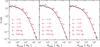 |
Fig. A.1 Mass distribution of clustered clumps with HDEs (left panel), with and without HDEs (middle panel), and without recomputing masses (right panel). For masses that are recomputed, we considered Eq. (6) and the ratio |
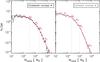 |
Fig. A.2 Mass distribution of clustered clumps (left panel) and isolated clumps (right panel) in the first quadrant. Only clumps with HDEs are used. The two plots correspond to the function Φ (Eq. (7)) versus mass. The red lines correspond to the fitting segments of the CMF. |
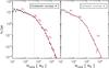 |
Fig. A.3 Mass distribution of clustered clumps (left panel) and isolated clumps (right panel) in the fourth quadrant. Only clumps with HDEs are used. The two plots correspond to the function Φ (Eq. (7)) versus mass. The red lines correspond to the fitting segments of the CMF. |
Appendix B: Catalogue tables
Partial list of cluster candidates. Columns (1)−(8).
continued. Columns (9)−(16).
Partial list of potential cluster candidates.
All Tables
CMF fitting results for clustered and isolated clumps in the whole sample, first and fourth quadrants.
All Figures
|
Fig. 1 Source density maps of a sub-sample of the three different types of clumps defined in the Hi-GAL product catalogue, located in the longitude range 26 ≤l≤ 31 deg. The same distributions are observed for the whole sample. |
| In the text | |
|
Fig. 2 Distribution of pre-stellar and proto-stellar clumps in a 2 × 2 square deg field centred on l = 330 deg. |
| In the text | |
|
Fig. 3 Distribution of the branch lengths found in the field displayed in Fig. 2. The grey line corresponds to the branch length histogram, whilst the black line is the cumulative distribution. The two dashed black lines are the fitted segments to the cumulative distribution. The dashed-dot line shows the cut-off branch length found at the intersection of these fits. |
| In the text | |
|
Fig. 4 Result of the MST method applied on the field in Fig. 2. Grey points and lines correspond to Λ > Λcut, whereas blue points and lines correspond to Λ < Λcut. Red lines correspond to convex hulls surrounding groups with N ≥ 10. |
| In the text | |
|
Fig. 5 Relation between Λcut and the mean density of the field considered. The red line corresponds to the correlation function |
| In the text | |
|
Fig. 6 Example of the reconstructing of the over-density catalogue found by the MST method at the split between windows. This example field is 10 deg large. Grey points are the pre-stellar and proto-stellar clumps. The grey shapes correspond to the convex hulls of the over-densities with at least ten members. The red shapes are the convex hulls of the over-densities split over the two original windows. The black dashed and solid lines mark the separation limits for each window. The top window is the overlap window. The middle windows are the two original windows of this field. The bottom window is the result of the overlapping method. |
| In the text | |
|
Fig. 7 Spatial distribution of the fraction of clustered clumps as a function of Galactic longitude. The black line corresponds to the mean fraction of clustered clumps of each master catalogue (one for each window size) for each 5 deg bin. The black points correspond to this mean and are located at the average longitude of each bin. The 1σ error bars correspond to the standard deviation of the fraction of clustered clumps for each bin. The grey dashed and dot-dashed lines correspond to a value of ±5% of Λcut. |
| In the text | |
|
Fig. 8 Variation of the fraction of clustered clumps into 2 × 2 square deg fields for all window sizes between 2 and 30 deg. |
| In the text | |
|
Fig. 9 Changes in the Λcut as a function of Galactic longitude in four different window sizes, with sizes of 2, 10, 20, and 30 deg. The Galactic longitude corresponds to the centre of each window. |
| In the text | |
|
Fig. 10 Longitude distribution of the 496 cluster candidates. The visible tangents of the spiral arms are located at l = 315 deg (black dashed line). The tangent at l = 295 deg is marked by a grey line. |
| In the text | |
|
Fig. 11 Top-down view of the Galaxy using the HDEs of the cluster candidates. The spiral arm model is supplied by Englmaier et al. (2011), with the different colour lines marking their locations. The plus (+) symbol represents the position of the Sun, with the grey dashed lines corresponding to Galactocentric distances. The black dots mark the location of the cluster candidates. The two grey shaded regions represent the regions where no cluster candidates could be found. |
| In the text | |
|
Fig. 12 Top: distribution of the mean scale height, Zmean, of cluster candidates as a function of Galactocentric radius. The black line corresponds to the cluster candidates in the first quadrant with the grey dashed line corresponding to the fourth quadrant. Bottom: distribution of the standard deviation, σZ, as a function of Galactocentric radius, R. |
| In the text | |
|
Fig. 13 Top: histogram of scale heights of the cluster candidates. The mean value is −6.2 pc. Bottom: distribution of cluster candidate Galactocentric radii. The peak is at ~6.5 kpc, a value also observed by Paladini et al. (2004). |
| In the text | |
|
Fig. 14 CMFs of clustered (left panel) and isolated (right panel) clumps. The masses of the clumps are computed using Eq. (6) and the ratio |
| In the text | |
|
Fig. 15 Highest mass clump in each cluster candidate as a function of total cluster mass. The grey dashed line is the 1:1 line and a highest value for the highest mass clump. The red line is the linear fit to the distribution. |
| In the text | |
|
Fig. 16 Distribution of the distance between clustered clumps in cluster candidates. The green dashed line represents the linear diameter of the beam at 70 μm. The orange dashed line corresponds to the same size, but at 500 μm. The grey line marks the Jeans length (0.1 pc). |
| In the text | |
|
Fig. 17 Cluster candidate properties as a function of mean clump mass. Top left: cluster density versus mean clump mass. Top right: mean MST clump length versus mean clump mass. Bottom left: cluster area versus mean clump mass. Bottom right: number of clumps versus mean clump mass. The colour bar corresponds to the heliocentric distance of the cluster candidate. |
| In the text | |
|
Fig. A.1 Mass distribution of clustered clumps with HDEs (left panel), with and without HDEs (middle panel), and without recomputing masses (right panel). For masses that are recomputed, we considered Eq. (6) and the ratio |
| In the text | |
|
Fig. A.2 Mass distribution of clustered clumps (left panel) and isolated clumps (right panel) in the first quadrant. Only clumps with HDEs are used. The two plots correspond to the function Φ (Eq. (7)) versus mass. The red lines correspond to the fitting segments of the CMF. |
| In the text | |
|
Fig. A.3 Mass distribution of clustered clumps (left panel) and isolated clumps (right panel) in the fourth quadrant. Only clumps with HDEs are used. The two plots correspond to the function Φ (Eq. (7)) versus mass. The red lines correspond to the fitting segments of the CMF. |
| In the text | |
Current usage metrics show cumulative count of Article Views (full-text article views including HTML views, PDF and ePub downloads, according to the available data) and Abstracts Views on Vision4Press platform.
Data correspond to usage on the plateform after 2015. The current usage metrics is available 48-96 hours after online publication and is updated daily on week days.
Initial download of the metrics may take a while.