| Issue |
A&A
Volume 596, December 2016
|
|
|---|---|---|
| Article Number | A47 | |
| Number of page(s) | 14 | |
| Section | Planets and planetary systems | |
| DOI | https://doi.org/10.1051/0004-6361/201629090 | |
| Published online | 28 November 2016 | |
Potassium detection in the clear atmosphere of a hot-Jupiter
FORS2 transmission spectroscopy of WASP-17b⋆
1 European Southern Observatory, Alonso de Córdova 3107, Casilla 19001, Santiago, Chile
e-mail: esedagha@eso.org; hboffin@eso.org]
2 Institut für Planetenforschung, Deutsches Zentrum für Luft- und Raumfahrt, Rutherfordstr. 2, 12489 Berlin, Germany
3 Zentrum für Astronomie und Astrophysik, Technische Universität Berlin, Hardenbergstraβe 36, 10623 Berlin, Germany
4 European Southern Observatory, Karl-Schwarzschild-Str. 2, 85748 Garching bei München, Germany
5 Astronomical Institute, Charles University in Prague, Vholešovičkách 2, 180 00 Praha 8, Czech Republic
6 Astronomical Institute ASCR, Fričova 298, 251 65 Ondřejov, Czech Republic
7 Department of Physics & Astronomy, University College London, Gower Street, London, WC1E 6BT, UK
Received: 10 June 2016
Accepted: 14 September 2016
We present FORS2 (attached to ESO’s Very Large Telescope) observations of the exoplanet WASP-17b during its primary transit, for the purpose of differential spectrophotometry analysis. We use the instrument in its Mask eXchange Unit (MXU) mode to simultaneously obtain low resolution spectra of the planet hosting star, as well as several reference stars in the field of view. The integration of these spectra within broadband and smaller 100 Å bins provides us with “white” and spectrophotometric light curves, from 5700 to 8000 Å. Through modelling the white light curve, we obtain refined bulk and transit parameters of the planet, as well as wavelength-dependent variations of the planetary radius from smaller spectral bins through which the transmission spectrum is obtained. The inference of transit parameters, as well as the noise statistics, is performed using a Gaussian Process model. We achieve a typical precision in the transit depth of a few hundred parts per million from various transit light curves. From the transmission spectra we rule out a flat spectrum at >3σ and detect marginal presence of the pressure-broadened sodium wings. Furthermore, we detect the wing of the potassium absorption line in the upper atmosphere of the planet with 3σ confidence, both facts pointing to a relatively shallow temperature gradient in the atmosphere. These conclusions are mostly consistent with previous studies of this exo–atmosphere, although previous potassium measurements have been inconclusive.
Key words: planets and satellites: atmospheres / planets and satellites: individual: WASP-17b / techniques: spectroscopic / instrumentation: spectrographs / stars: individual: WASP-17 / methods: data analysis
The data of the light curves are only available at the CDS via anonymous ftp to cdsarc.u-strasbg.fr (130.79.128.5) or via http://cdsarc.u-strasbg.fr/viz-bin/qcat?J/A+A/596/A47
© ESO, 2016
1. Introduction
In the short number of years in which extrasolar planetary systems have been detected and studied, great progress has been made in understanding these alien worlds and characterising their intrinsic properties. Methods such as radial velocity and transit monitoring, have facilitated the measurement of bulk densities, as well as some initial approximations of the structure and atmospheric properties of extrasolar planets. We are concerned with the latter here, whereby spectroscopic observations of exoplanetary primary transits lead to setting constraints on the chemical composition and physical processes within exo-atmospheres.
Through transmission spectroscopy, we analyse the wavelength-dependent variations of the exoplanetary radius. These minute variations are caused by the presence of an optically thick atmosphere at specific wavelengths, dictated by the absorption and scattering characteristics of the gas and aerosols that are present near the planet’s terminator. These wavelength-dependent opacity variations are scanned across the spectrum and used to probe chemical compositions of the planets’ atmospheres (Seager & Sasselov 2000; Brown 2001). The ideal candidates for such studies are those planets with extended atmospheres, i.e. with large atmospheric scale heights, such as the so-called hot Jupiters (Seager & Sasselov 1998). The search for signatures of exo-atmospheres began as early as the time when predictions were being made. For instance Rauer et al. (2000) and Harris et al. (2000), among others, looked for spectral signatures that were due to absorption by extended atmospheres surrounding 51 Peg b and τ Boötis Ab.
Traditionally, transmission spectroscopy has been dominated by space-based facilities, because of their obvious advantage of not being affected by telluric extinction (Charbonneau et al. 2002; Ehrenreich et al. 2007; Pont et al. 2008; Gibson et al. 2012a; Deming et al. 2013; Knutson et al. 2014; Swain et al. 2014). However, large ground-based telescopes, with instruments meeting the requirements of transmission spectroscopy science goals such as the VLT/FORS (Appenzeller et al. 1998), Gemini/GMOS (Hook et al. 2004) or Magellan/IMACS (Bigelow et al. 1998) have been the most effective and have also been able to contribute to such studies. Gibson et al. (2013a,b), among others have shown the capabilities of GMOS to produce transmission spectra for a number of transiting hot Jupiters. With its Multi Object Spectroscopy (MOS) and Mask eXchange Unit (MXU) modes, the FOcal Reducer and low dispersion Spectrograph (FORS2) instrument on the Unit Telescope 1 (UT1 – Antu) of ESO’s Very Large Telescope (VLT) has also been a key player in producing these type of spectra. Bean et al. (2010, 2011) were able to obtain pioneering results for the GJ1214b transmission spectrum, an exoplanet in the mini Neptune regime, from the visible to near-infrared bands. However, subsequent attempts at transmission spectroscopy analysis with this instrument were mostly unsuccessful owing to systematics present in the data associated with prisms of the Longitudinal Atmospheric Dispersion Corrector (LADC). Therefore, a project was started at ESO Paranal to address these issues (Boffin et al. 2015) by removing the inhomogeniously degrading coating from the prisms of the decommissioned FORS1’s LADC, replacing them with their FORS2 counterpart. The improvements were subsequently highlighted through transit observations of WASP-19b, the results of which were presented in Sedaghati et al. (2015).
An essential issue, which plagues all the aforementioned instruments, has been the role of instrumental systematics and their manifestation in the final transit light curves. As transmission spectroscopy heavily relies on the extremely precise measurement of the transit depth (a few hundreds of ppm1 for hot Jupiters, down to a few ppm for terrestrial planets) and subsequently the relative planetary radius, the consideration of such factors is crucial when determining the correct scaled radius values, as well as pragmatic estimation of their error budgets. This fact is of paramount importance when a transmission spectrum is used together with atmospheric models in determining the physical properties of an exo-atmosphere. The time-dependent correlated noise2 that is due to systematics is somewhat reduced through differential spectroscopy techniques employed in this work, however some effects are still expected to remain that originate from poorly understood sources. With this apparent correlated noise component in mind, we utilise a method to model and analyse transit light curves in this paper. The method is based on the Gaussian process (GP) of Gibson et al. (2012b), adapted for modelling time-correlated noise, which has been shown to provide conservative and realistic error estimations (Gibson et al. 2013b) as compared to other parametric methods such as the wavelet decomposition techniques of Carter & Winn (2009). This is an essential point to consider when detecting exoplanetary atmospheric features with transmission spectroscopy, since underestimating the precision of radius measurements can lead to the false or inaccurate characterisation of the atmosphere.
Here we report FORS2 observations of WASP-17b in MXU mode. WASP-17b (Anderson et al. 2010) is an ultra low density Jupiter-sized planet on a ~3.74 d, possibly retrograde orbit around an 11.6V magnitude F6V star. It has a mass and radius of 0.486 ± 0.032 MJupiter and 1.991 ± 0.081 RJupiter respectively (Anderson et al. 2011), making it an extremely bloated hot Jupiter at only 0.06 ρJupiter. This, together with an equilibrium temperature of 1771 ± 35 K (Anderson et al. 2011), mean a relatively large atmospheric scale height, making it an ideal candidate for transmission spectroscopy studies.
This paper is structured as follows. Section 2 highlights our observations and data reduction, in Sect. 3 we present detailed transit data analysis steps, in Sect. 4 we show the results of the analysis and discuss the atmospheric characteristics of WASP-17b, in Sect. 5 we briefly discuss our atmospheric results for this exoplanet, and finally in Sect. 6. a brief summary of our conclusions is presented.
2. FORS2 observations
A single transit of WASP-17b was observed using the 8.2 m UT1 of the VLT with the FORS2 instrument on the 18 June 2015, with the data taken as part of the programme 095.C-0353(A) (PI: Sedaghati). FORS2 has a 6.8′ × 6.8′ field of view, including a detector system consisting of a mosaic of two 2k × 4k, red optimised, MIT CCDs, utilised for the observations, all of which are visible in Fig. 1. We used FORS2 in the MXU3 mode to observe the target and a number of reference stars simultaneously for ~8.1 h, covering the 4.38 h of complete transit plus 2.3 h prior to ingress and 1.4 h post egress. Observational conditions were clear for parts of the night, with some sporadic cirrus affecting the observations in transit. The LADC was left in park position during the observing sequence, with the two prisms fixed at their minimal separation distance of 30 mm. At the start of the observations (23:20 UT), the field was at airmass of 1.48, moving through the zenith at 00:23 UT and finally settling to 2.31 for the last exposure at 07:45 UT.
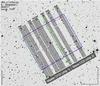 |
Fig. 1 10′× 10′ plot encompassing the FoV of FORS2 (green box) and the area covered by the 2 (2k × 4k) MIT chip mosaic (in blue). The exact design and location of the MXU slits, with the relevant target designations are also shown. The grey regions are the sections of the CCD used for recording the individual stellar spectra. |
The observations were performed with the 600RI grism plus the GG435 order sorter filter, covering the wavelength range4 of ~5500 to 8300 Å. The exposure times were 35s throughout the night and the data were binned (2 × 2) yielding a scale of 0.25′′ per pixel. We used the non-standard 200kHz readout mode, enabling us to spend more time on target for a fixed cadence (~70 s), owing to the reduced readout time and lower gain of this mode. This procedure resulted in 477 exposures, with some time lost to resetting the field rotator, which we ensured was performed pre-ingress. We created a customised mask with 15′′ wide slits to minimise slit losses. The slits were mostly 30′′ long, with the exception of two to avoid overlapping dispersion profiles. The mask set up on the sky is shown in Fig. 1. A copy of the mask was created for the purpose of wavelength calibration, with narrow 1′′ slits centred on the science slits. Bias, flatfield and arc images were taken, as part of the routine daytime calibration sequences, before and after the observations. Details of an optimised observational strategy with FORS2 have been presented by Boffin et al. (2016).
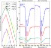 |
Fig. 2 Left: cross-correlation functions, calculated for the wavelength solutions of all reference stars, with respect to the target. The maximising wavelength at each instance, presented in the figure, is then added to each wavelength solution for the correction of the spectra. Right: a zoom into the telluric O2 absorption region of the spectra, before and after the wavelength correction procedure. |
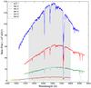 |
Fig. 3 Wavelength-corrected raw spectra of the target and reference stars, where the numbers are consistent with those in Fig. 1. The grey shaded region represents the integration limits for the broadband light curve production. |
3. Data reduction and analysis
We wrote a PyRAF5 pipeline for the reduction purposes of the data, optimising it to the specific science goals of this dataset. The steps in the pipeline included the overscan and bias shape subtraction, spectral flat-fielding and wavelength calibration. Subsequently, wavelength-calibrated spectra were extracted for the target and five of the seven reference stars, while simultaneously subtracting the sky background and removing any cosmic ray contamination. We also needed to finely tune the dispersion solution found for the reference stars owing to the imperfect centering of stars on the slits. This was done by cross correlating the spectrum of each reference star with that of WASP-17, shown in Fig. 2, to find a small shift between each pair. The maximal solution was then added to the wavelength stamp of each reference star’s dispersion relation. This is a rather important point to consider, since differences in wavelength solutions of various stars could cause artificial features in the spectrophotometric light curves. An example set of these extracted spectra is shown in Fig. 3. A careful analysis of the choice of reference star and its impact on the final light curve is presented in the following section.
3.1. Reference star analysis
We observed a total of eight targets through the custom designed mask, with wide slits placed on those targets. Of the seven reference stars, five were deemed bright enough for further analysis. We searched through a variety of catalogues for estimation of the spectral type of these stars, the results for which are given in Table 1. Furthermore, we also searched through a number of catalogs for variability in our reference stars. From the Catalina survey (Drake et al. 2009), the star in slit 3 shows periodicity at ~4.4 days at an amplitude of ~0.1 mag. However, this result is rather tentative since the object is brighter than the 13 Vmag saturation limit given by the survey. Additionally, the duration of our observations is considerably shorter than the variability period and therefore any possible intrinsic variation should be insignificant for our purposes.
Spectral characterisation of the stars observed.
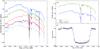 |
Fig. 4 a) Raw time-series light curves of the six stars observed and analysed with the custom designed mask, shown in Fig. 1. b) Raw light curves for WASP-17 and the composite comparison star made from the combination of all reference stars, excluding reference 4. c) Normalised transit light curve for WASP-17b obtained through division of the two plots above and normalised to out-of-transit flux mean. Light curves in panels a) and b) have been shifted for clarity. |
We first integrate the individual spectra for the largest possible common wavelength domain of all six targets to produce the raw broadband light curves shown in Fig. 4a, normalised to the mean flux and shifted for clarity. We then produce differential light curves by simply dividing the normalised WASP-17 light curve by all the individual reference stars (Fig. 4b), as well as all possible multiple-star combinations. The final comparison star is created through the combination of all reference stars, excluding reference star 4, since its inclusion results in a transit light curve with larger systematics, as well as reducing the possible wavelength domain available for integration of spectra. We also experimented with a composite comparison star that was obtained using a weighted mean of all the individual reference stars using the signal to noise ratio (S/N) of individual transit light curves as the weights. However, this did not have any impact on the final transit light curve. Hence, we create the final comparison using the arithmetic mean of the chosen reference stars (2, 3, 5, and 6).
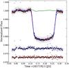 |
Fig. 5 Broadband (white) light curve for the transit of WASP-17b, fitted with a GP model described in Sect. 3.3. The best fitting transit light curve is shown in blue with the GP mean model given as solid red line. The residuals of both models are shown at the bottom, where they are shifted for clarity and their colours correspond to the models that they represent. The dark and light grey regions represent the 1 and 3σ predictions of the GP model, respectively. The green line shows the systematics model without the transit function. |
3.2. Spectral statistical analysis
To obtain the wavelength dependency of planetary radius, we need to produce spectrophotometric light curves. This is done by integrating the obtained spectra within arbitrarily positioned filters of widths that are based on the quality of the light curves produced. Typically, transmission spectra produced with FORS2 have resolutions of 200 Å (Bean et al. 2010; Sedaghati et al. 2015), with the exception of a few studies (e.g. Bean et al. 2011; Lendl et al. 2016) that produced spectra with 100 Å bands. The precisions of differential and detrended light curves are calculated for a range of bandwidths, measured across the entire wavelength domain. This is done by calculating the dispersion of the normalised foot for light curves produced at a central wavelength λc and bandwidths6δλ in the range of 20−300 Å. This process is performed for the entire wavelength range, for λc values spaced at 50 Å. Subsequently, to interpolate the results in between these steps, we apply a Gaussian convolution filter for a smoothed continuous dispersion map7. This is essentially similar to the mean filter, but having a different kernel, an application for which is given by Buades et al. (2005) for image denoising. The results from such statistical analysis of light curve precision across the entire spectrum is shown in Fig. 6.
It is quite evident, that in certain regions, a rather large bandwidth is required to obtain a precise light curve. This is due to the presence of telluric absorption features that reduce the signal-to-noise ratio in the produced light curve significantly. Based on this analysis and taking into account the contours of Fig. 6, we choose 100 Å as the bandwidth to be used for the production of the spectrophotometric light curves. This value is chosen to provide us with high-resolution transmission spectral points that are simultaneously precise enough for comparison with atmospheric models.
3.3. Transit light curve fitting
Once the final normalised broadband and spectrophotometric light curves are produced (see Figs. 4, 5 and 7), we first infer all the transit parameters, as well as the noise characteristics of the broadband light curve. Subsequently, the same procedure is repeated for the spectrophotometric light curves with only the wavelength-dependent transit parameters and noise components inferred, while others are fixed to the white light curve solution, since it represents the light curve with the highest S/N, and hence the most accurate solutions.
We fit all the light curves using a Gaussian process (GP) model, whose application to modelling systematics in time-series data was introduced by Gibson et al. (2012b). To determine the GP model, we made use of their GeePea module, as well as the Infer module to implement Bayesian inference routines8.
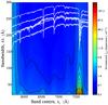 |
Fig. 6 Analysis of light curve precision across the entire wavelength domain, with the spectra of WASP-17 and all reference stars superimposed at the top. Clearly, the regions containing telluric absorption features, require larger bandwidths to produce reasonable spectrophotometric light curves, for instance the O2(A) absorption region at approximately 7600 Å. |
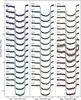 |
Fig. 7 Spectrophotometric light curves for the transit of WASP-17b, produced with bins of 100 Å width after the common mode correction (CMC), shifted for clarity. The solid black line for each plot is the best-fit transit systematics model and the grey areas are the 1σ representations of those solutions. The dashed lines represent transit models derived with the optimised parameters of each light curve. The central wavelength of each channel used to produce the light curve is given next to each plot. The light curves excluded from transmission spectroscopy have been included here for completeness. |
A GP is essentially a non-parametric approach to regression analysis that does not necessarily make any assumptions about the data, nor does it impose a deterministic model on the data9. It is simply a collection of random variables, any finite subset of which has a joint Gaussian distribution (Gibson et al. 2012b). In this framework, each light curve is modelled as a GP of the analytical transit function, following the formalism of Mandel & Agol (2002), and the covariance matrix representing the noise characteristics of the data: ![\begin{equation} \label{eq:GP} f(t,\boldsymbol{\phi},\boldsymbol{\theta}) \sim \mathcal{GP}\left[T(t,\boldsymbol{\phi}),\boldsymbol{\Sigma}(t,\boldsymbol{\theta})\right] \end{equation}](/articles/aa/full_html/2016/12/aa29090-16/aa29090-16-eq25.png) (1)with f being the flux measurements and t the time of each observation. Here T is the analytical transit model that is a function of t and the transit parameters φ. In addition, Σ represents the covariance matrix, whose kernel has time as its only input, with parameters θ also known as the hyperparameters. We also extracted as many physical variants, also known as the optical state parameters, as available, to search for any correlations between them and the residuals of a transit model fit to the data. However, owing to the lack of any correlation none of this information was used in describing the GP model. Some of the extracted data are shown in Fig. 8.
(1)with f being the flux measurements and t the time of each observation. Here T is the analytical transit model that is a function of t and the transit parameters φ. In addition, Σ represents the covariance matrix, whose kernel has time as its only input, with parameters θ also known as the hyperparameters. We also extracted as many physical variants, also known as the optical state parameters, as available, to search for any correlations between them and the residuals of a transit model fit to the data. However, owing to the lack of any correlation none of this information was used in describing the GP model. Some of the extracted data are shown in Fig. 8.
The covariance matrix in Eq. (1) is given by  (2)where ζ is the output scale describing the GP’s variance, l is the length scale that determines how smooth the function is, δ is the Kronecker delta ensuring the addition of white noise to the diagonal of the covariance matrix and σw is that Poisson noise. For the covariance function or the kernel, k(ti,tj,θ), we have chosen the squared exponential (SE) kernel (e.g. Wilson & Adams 2013) owing to the smoothness of the function over the parameters. We emphasise that although selecting a kernel is analogous to choosing a predetermined parametric model, it allows for a much more flexible treatment of noise than any parametric form, as well as being intrinsically Bayesian.
We also define priors for all the hyperparameters of the noise model, ensuring that their values are positive, and together with the mean transit function parameters, optimise them with a Nelder-Mead simplex algorithm (Glaudell et al. 1965). To obtain the posterior joint probability distributions, these are multiplied by the marginal likelihoods of producing the joint posterior probability distribution. In other words,  (3)We then use Monte Carlo Markov Chains (MCMC) to explore this posterior distribution and produce the final marginal probabilities for each of the parameters (for both the transit and the noise models). Essentially, we just assume uniform, uninformative priors for all the parameters with few restrictions, i.e. the impact parameter10 and GP hyperparameters are positive and the sum of the two limb darkening coefficients of the quadratic law are less than unity to ensure positive brightness across the entire stellar surface. For all the light curves we ran four MCMC chains with 100 walkers of 100 000 iterations. Once the chains are computed, we extract the marginalised posteriors for the free parameters to check convergence and any correlations. Examples of these correlation plots and posterior probability distributions are shown in Fig. 9 for the broadband and one spectrophotometric light curve.
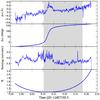 |
Fig. 8 Some of the optical state parameters extracted from the data. From the top, Δx is the spectral drift relative to the first exposure, calculated using cross-correlation of the raw spectra, Δφ is the instrument rotation angle, seeing is measured as the product of full width half maximum from the Gaussian profile along the spatial axis and the pixel scale in arcsec and X is the airmass. These parameters are extracted to check for any possible correlation with the systematics in the light curve. The grey shaded region shows the duration of transit. |
4. Results
4.1. Broadband light curve models
We first model the broadband or white light curve, which is the integral of fluxes for the largest possible common wavelength domain of the target and the comparison, namely from 5700 to 8000 Å, as shown in Fig. 5 and modelled with the quadratic limb darkening law (Kopal 1950). To ensure that the choice of limb-darkening law does not have a significant impact upon the inference of transit parameters, we initially model the white light curve using both the quadratic Iquad(μ) and the non-linear law Inl(μ) (Claret 2000), also known as the four-parameter law, given by  respectively, where μ (=cosθ) is the cosine of the angle between the observer and the normal to the stellar surface. These formulations have as particular cases, the linear law (Schwarzschild 1906, c2 = 0 in the quadratic law) and the three-parameter law (Sing et al. 2009, l1 = 0 in the non-linear law). To initially examine the impact of the chosen limb-darkening law on the inferred planetary radius, we model the broadband light curve with the aforementioned laws, taking a variety of approaches for coefficient determination. Beyond the quadratic law, no improvement is made to the fit when using a more complex law and there are no significant changes in the inferred transit parameters. Furthermore, high levels of correlation exist between the fitted parameters of those laws. This together with the added unjustified complexity means that the quadratic law is chosen to model the radial intensity variations across the stellar disk.
In our modelling process, both coefficients of the quadratic limb-darkening law are fitted for in the white and spectral channels, since the stellar intensity profile is expected to be colour-dependent. To determine these coefficients, we impose some informative priors. The first of these restrictions is that the sum of their values is less than unity to ensure a positive value for the stellar surface intensity across the entire disk. Initially, we calculate coefficient values for all channels using the PyLDTk11 package (Parviainen & Aigrain 2015), which uses the stellar atmosphere tables of Husser et al. (2013) generated with the PHOENIX code. We initially use these values to construct Gaussian priors for the inference of the coefficient values from the MCMC analysis, using the calculated values as the mean and twice the error as the standard deviation. However, this approach is rather restrictive and leads to systematic errors in the final fit. Hence, we use these calculated values to construct a global and less informative prior given by  The optimised parameters and the noise characteristics from fitting the broadband light curve, with the above-mentioned setup, are given in Table 2. Through the combination of multiple reference stars, the colour-dependent slope in the white light curve dispears, and hence we do not include a polynomial fit of the foot points. This, however, is not the case for the narrowband channels. These inferred planetary transit parameters from the MCMC analysis are consistent with those reported previously (Anderson et al. 2010, 2011; Southworth et al. 2012; Bento et al. 2014).
Parameters from the MCMC analysis of the broadband light curve, given for the fully marginalised Gaussian process noise model.
4.2. Transmission spectrum
Once the system parameters are determined from the analysis of the broadband light curve, we model the spectrophotometric light curves in the same way, but with the non-wavelength dependent parameters fixed to the best solution from the white light curve, which is given in Table 2. Since this light curve represents the time-series flux measurements with the highest S/N, its solutions are the most trust-worthy. In modelling the spectroscopic light curves, we fit for the scaled planetary radius (Rp/R⋆), both coefficients of the limb-darkening law, c1 and c2, as well as the three quantities that describe the noise statistics of each data set, ζ, l and σw, as explained above. In addition to those, in the modelling of spectrophotometric light curves, we also simultaneously fit for three coefficients of a second order polynomial, which approximates long-term trends in the differential flux. Such variations are due to larger colour differences between the target and the comparison in smaller bins as compared to the broadband bin, where such effects are not apparent. This effect is a function of airmass and spectral type described well with a polynomial of second order, which can be seen in some of the light curves in Fig. 7. An example of the correlation plots for the free parameters of one spectral light curve is shown in the upper panel of Fig. 9.
As well as this approach, we also correct the spectrophometric light curves for a common mode of the systematic noise that is shared across all the spectral channels. This is done by dividing all the spectrophotometric light curves by the residuals of best-fit transit model to the broadband light curve, shown as the blue data points at the bottom of Fig. 5. This residual data is simply obtained by the division of the transit data by the analytical model (blue solid line in the top figure of the same plot). Subsequently, we model these light curves again with the same procedure, where the red noise is modelled as a GP owing to any residual systematic noise after this common mode correction (CMC). These light curves together with the transit and GP noise models are shown in Fig. 7.
The variations of relative planetary radii as a function of channel central wavelength, λc, are derived from this modelling process, which represents the transmission spectrum of WASP-17b. A set of results from modelling of both data sets (initial and CMC), including relative radii and limb-darkening coefficients, are tabulated in Table 3. The transmission spectrum is shown in Fig. 10 for the two employed procedures.
One possible feature of these spectra is the indication of enhanced absorption in the exoplanetary atmosphere in the range of 7650−7800 Å, which is possibly due to a combination of the telluric O2(A) lines and the Potassium doublet (7665 Å and 7699 Å) in the exoplanet’s atmosphere. This point will be discussed further in Sect. 4.3. To look for possible optical absorbers in the atmosphere of WASP-17b, we also produce narrow band light curves with 50 Å integration bins around Sodium and Potassium absorption regions, which are shown in Fig. 11.
Results from modelling spectrophotometric light curves produced with 100 Å integration bins, for both data sets.
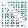 |
Fig. 9 Parameter correlations for the broadband (bottom left) and a spectrophotometric (top right) light curve from the MCMC analysis, for the quadratic limb-darkening law. The well-documented degeneracy between the impact parameter, b, and the scaled semi-major axis, a/R⋆ is also quite evident. The derived posterior probability distribution for each parameter is also given at the end of each column. The four different colours represent samples from the independent MCMC chains. |
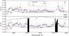 |
Fig. 10 Transmission spectrum of WASP-17b produced from both without (top) and with (bottom) the CMC of the spectrophotometric light curves. Blue circles and red triangles are the results from light curves made with 100 Å bins, plotted as two separate sets to show transmission spectra with unique data points. Furthermore, synthetic transmission models for the reference aerosol profile scaled by factors of 0, 10, 100 and a 1000 are also overplotted. These models are binned within 100 Å channels to match the data. In the CMC plot, an example of a WASP-17 spectrum is overplotted in grey. Two regions of telluric absorption have been shaded black, where we avoid reporting results due to the low S/N. We emphasise that the models are not fitted to the data and simply just overplotted. Hence, we do not try the retrieval approach since the wavelength coverage of the spectrum is too limited for this approach. |
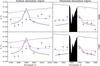 |
Fig. 11 Transmission spectrum reproduced with 50 Å-wide bins, as compared to Fig. 10, for domains where the possible presence of optical absorbers, such as sodium (left column) and potassium (right column), would result in an increased planetary radius. The theoretical atmospheric models are also overplotted in addition to the inferred radii, and their colours correspond to those in Fig. 10, which have again been binned to the resolution of the spectrum and plotted for 1.6 scale heights, as was performed for the overall spectrum. It must be noted that these models have not been fitted to the data points and the transmission spectrum data have not been used as a priori for the production of the model atmospheres. The black shaded region in the right column highlights the region where telluric absorption as a result of the O2 (A) lines introduces significant systematics in the light curves produced in this region. |
4.3. Atmospheric models
We compare the derived transmission spectra of Fig. 10 to especially adapted theoretical atmospheric spectral models also shown in the same figure. These models are calculated with the assumption of isothermal profile using the equilibrium temperature of WASP-17b, as well as full heat redistribution and zero albedo. The only spectroscopically active gases present in the model atmosphere are H2O, Na, and K, with volume mixing ratios of 1 × 10⁻³, 2.96 × 10⁻⁶, and 2.4 × 10⁻⁷, the latter two being solar values that assume H2/He bulk abundances and the water mixing ratio being somewhat arbitrary. These mixing ratios are assumed as being independent of altitude. We take the specific gravity to be non-constant and varying with altitude, since this probably would be significant for a puffy and low density planet like WASP-17b. Furthermore, we assume that the aerosol density decays with altitude using a scale height similar to that of the gas. To explore the impact of aerosol density, we have scaled the reference aerosol profile (× 1), by factors of 0, 10, 100, and 1000, which are all shown in Fig. 10, superimposed onto the derived transmission spectra. In these cases, the aerosol optical thickness of 1 at 0.8 micron is reached at pressure levels of ~7, 1, 0.15, and 0.03 bars, respectively. This aerosol optical thickness is assumed to follow a Rayleigh-type law with a wavelength dependence of λ-4. This law is valid when the size parameter x (=2πreff/λ; where reff is a measure of the particle radius) is quite small and the imaginary part of the refractive index is also small. For instance, silicates, perovskite, and silica have small imaginary parts for their refractive indices. This is a hard-coded assumption of the model, but is anyway consistent with the Rayleigh slope that is seen in numerous exoplanets. WASP-17b has a rather puffy composition, hence one would expect that small particles are easily kept aloft in the atmosphere. Given the very unconstrained nature of the problem, we think that the treatment used here is judicious. Finally, given the fact that the extinction coefficient decays exponentially with altitude, and the pressure levels at which maximal optical thickness is reached (i.e. τ = 1), one reconstructs the aerosol extinction coefficient needed in the models12. These theoretical atmospheric models are updated versions from García Muñoz et al. (2012).
The plotted theoretical models have been shifted vertically to match the visible size of the planet and scaled by ~1.6 scale heights, a value which has been obtained through minimization of χ2 statistics using least squares with transmission spectrum data points.
We calculate χ2 and significance statistics using the CMC spectrum of Fig. 10 to establish whether one can discriminate between a clear or cloudy and opaque atmosphere. To do this, the synthetic spectra are compared to a flat spectrum with a one scale-height tolerance. We calculate a reduced  value of ~1.19 for a flat spectrum, compared to ~1.07–1.11 for the various atmospheric models. Hence, we rule out a flat spectrum at >3σ, with the ΔBIC (≫10)13 value providing further, very strong evidence against it. Details of the statistical analysis of the individual models are given in Table 4. From this analysis, we conclude that our transmission spectrum significantly rules out a flat spectrum and suggests an atmosphere clear of large cloud particles for WASP-17b, with the possible presence of smaller scattering particles, since there is marginally a better agreement of data with the models of increased aerosol density.
Calculated statistics for the various models overplotted with the data.
Following the recipe of Nascimbeni et al. (2013) and Mallonn & Strassmeier (2016), we estimate the mean molecular weight of the atmosphere using a fitted Rayleigh slope, from the relation  (6)where H is the scale height of the atmosphere, α = −4 for Rayleigh scattering, kB is the Boltzman’s constant, Teq the exo-atmosphere’s equilibrium temperature, μm is the mean molecular weight of that atmosphere and gp is the planetary surface gravity. We estimate the Rayleigh scattering slope using the CMC transmission spectrum. Owing to larger uncertainties at either extreme of the spectrum, as well as telluric effects and possible absorption by exoatmospheric gases, we only include data points from 6100 to 7500 Å for the calculations. The slope is subsequently obtained through a weighted least squares fitting method, giving the best-fit value of
 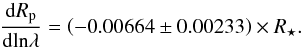 (7)Using the stellar radius value from Anderson et al. (2011), we obtain a mean molecular weight, μg, of 2.05 ± 0.79 atomic mass unit (a.m.u.) for Bond albedo of 0, and 1.88 ± 0.73 a.m.u. for αB = 0.3, which has been shown to be a reasonable upper limit for hot gas giants (Spiegel et al. 2010; Esteves et al. 2013). These values are generally consistent with a mostly H2 dominated atmosphere, but owing to the large uncertainties in determination of Rayleigh scattering slope, they could also point to the presence of H or He. However, a lack of H-α absorption in the transmission spectra somewhat rules out the former.
We also perform a similar analysis for the additional spectra created around the sodium and potassium absorption lines with narrower bins of 50 Å, shown in Fig. 11 to determine the significance of any possible detection. Wood et al. (2011) detect an increases in transit depth of 1.46%, 0.55%, and 0.49% for 0.75 Å, 1.5 Å, and 3 Å bin, respectively. However, they report no significant detection for bins of 4 Å and higher. Hence our non-detection of increased absorption in the Na core with the 50 Å bin is consistent with their results. Similar conclusions were also made by Zhou et al. (2012), where transit depth increase of 0.58% was detected in the Na core using a 1.5 Å bin. Taking only the points around the sodium line in Fig. 11 into consideration, we calculate a marginal improvement (~1σ) to a fit, when a flat spectrum is compared to a model with sodium absorption included. Presence of pressure broadening would point to a rather shallow temperature gradient, although more precise measurements of the planetary radius at higher resolution are required to confirm this result. More recently, Sing et al. (2015) also detected increased absorption in the sodium core using the Space Telescope Imaging Spectrograph (STIS) instrument on-board the Hubble Space Telescope (HST), using a narrow bin. Using very small integration bins placed on the core of the absorption line only probes the lower atmosphere (Wood et al. 2011), as opposed to larger bins where the diminished signal could be due to the presence of silicate and iron clouds increasing the opacity (Fortney et al. 2003). The absence of sodium from high altitudes can be explained for equilibrium temperatures below ~1000 K, where atomic Na is lost to the formation of various compounds and rained out of the upper atmosphere (Burrows et al. 2000), but this is not the case for WASP-17b. Lavvas et al. (2014) provide yet more possible explanations for the presence and/or absence of Na and K in giant exoplanet atmospheres.
Similarly we also search for potassium absorption in the atmosphere of WASP-17b, obtaining and analyzing light curves using 50 Å integration bins. Unfortunately, the majority of the potassium doublet core falls on top of the telluric O2 (A) absorption lines, as shown in the right column of Fig. 11, which introduce large systematics for light curves obtained in this region. Hence, we avoid producing and analyzing transit light curves in this domain where the signal is diminished by the Earth’s atmosphere. However, since the potassium core falls close to the red edge of the telluric forbidden region, we are able to probe and detect the red wing of the pressure-broadened line. Using the data points redwards of the telluric absorption in Fig. 11, we find a 3σ improvement to the fit when a flat spectrum is compared to the atmospheric models including potassium. To date only one previous work has looked at this domain of the spectrum (Sing et al. 2015), where the narrow bin placed at the core of the potassium line is inconclusive in determining its presence or absence. Given that potassium is present in the atmosphere of WASP-17b, the pressure broadening of its wings would be consistent with what we observe for the sodium line.
Charbonneau et al. (2002) first report detection of Na in HD 209458b. Subsequent studies suggested that the Na absorption was weaker than estimated by theory (Seager & Sasselov 2000) and that the potassium signal was lacking (Snellen et al. 2008) for this planet. Four factors have been suggested that could influence the spectral bands of the alkali metals, Na and K: (i) an elemental abundance different from the commonly assumed solar value; (ii) masking by atmospheric hazes; (iii) in situ photochemical reactions; and/or (iv) condensation, e.g. on the planetary night side.
Lavvas et al. (2014) review processes affecting Na and K signals in hot Jupiter atmospheres and apply a photochemical model including in situ Na and K reactions. Regarding the effect of elemental abundances, they suggested values up to 6× lower than the solar value for Na and K, for example, for HD209458, based on stellar metallicity measurements. Regarding the masking of spectral bands, they note that it is difficult to mask only the sodium line (and not the potassium line) since sodium is a strong absorber; this could however be achieved in the presence of certain hazes although the size distribution of the haze particles would have to be consistent with the observed Rayleigh slope. With regards to in situ photochemistry, two important species that are formed are: XH (formed via: X+H2) and XOH (formed via X+H2O) (where X=Na, K). Both XH and XOH can then undergo thermal decomposition to re-generate the alkali metal atoms (X). Uncertainties in the photochemistry include, for instance, reactions of potassium (e.g. here the three-body combination rates are not well known and one usually assumes the same coefficients as for sodium); also at hot-Jupiter temperatures, excited states could become important, the photochemical responses of which are not well-defined. Lavvas et al. (2014) conclude that the uncertainties in photochemistry however, are small compared with the potential effect of masking by hazes. Regarding condensation of alkali metals on the night-side, more work is required on, for example, the 3D transport mechanisms across the terminator.
5. Conclusions
We have presented the transmission spectrum of the hot Jupiter, WASP-17b, using the FORS2 instrument at ESO’s VLT, in its multi-object spectroscopy mode. Using a combination of light from multiple comparison stars, we obtained the broadband differential transit light curve of this planet, whereby the bulk orbital and physical parameters were derived.
From the broadband light curve, we obtained refined non-wavelength-dependent transit parameters, which are consistent with previous analyses (Anderson et al. 2011; Southworth et al. 2012; Bento et al. 2014). Through detailed study of parameter inference and correlations, we modelled all the obtained light curves using the quadratic limb-darkening law for the host star.
Spectrophotometric light curves are analysed as independent GP noise models together with an analytical transit function, where strict, delta-function, priors for non-wavelength-dependent parameters were assumed, based on the broadband solution. We explored the posterior distribution for the remaining free parameters, these being the scaled radius, the two coefficients of the limb darkening law, noise model parameters and three coefficients of a second order polynomial, which describes the colour-dependent out-of-transit flux variations, to quote the best-fit solutions as a function of channel wavelength. We take a non-parametric approach to modelling the time-correlated noise in the data, with time taken as the only input of our GP model (Gibson et al. 2012b) in calculation of the covariance matrix. This procedure was performed on two sets of light curves, where for the second set (CMC), we applied what is known as the common mode correction by removing the systematic noise common to all the wavelength channels.
Through a comparison of transmission spectra (produced from both sets of light curves) with synthetic atmospheric models, we rule out a cloudy makeup of WASP-17b’s upper atmosphere with high significance (>3σ). From fitting a Rayleigh scattering slope, we estimate an atmosphere with a mean molecular weight consistent with the prevalence of H2. Further observations with the 600B grism of FORS2, extending the spectrum towards the ultraviolet, will be required to confirm and quantify this aspect of the exo-atmosphere with higher precision.
Additionally, we looked closer at the possibility of enhanced absorption towards the two main optical absorbers, sodium, and potassium. We do not detect a significant variation of the planetary radius at the sodium core with a 50 Å bin, consistent with previous conclusions of Wood et al. (2011) and Zhou et al. (2012). Owing to the low significance levels, we are not able to confirm nor rule out the presence of the pressure-broadened wings of the sodium absorption line. Further, higher precision and resolution observations will be required to confirm this feature. Similar conclusions are made for potassium, although we were not able to probe the absorption in the core of the line owing to the telluric O2 feature. However, we do confirm the presence of the pressure–broadened wing of the potassium line with 3σ significance, which amounts to a significant detection.
Ultimately, our observations and analysis highlight the importance and capability of ground-based facilities in detecting and characterising exoplanetary atmospheres. FORS2 will play an important role in those efforts, providing the wider community with an essential outlet for follow-up of fascinating current and future targets.
We start at 20 Å minimum bandwidth, since below this integration size the algorithm that detects the transit locations automatically, runs into difficulty, due to the low S/N in the light curve. Furthermore, for practical purposes, the calculations are performed with steps in bandwidth of 10 Å to reduce computation time.
The modules used are available at the following repository: https://github.com/nealegibson
Available from https://github.com/hpparvi/ldtk
Bayesian Information Criterion (Schwarz 1978).
Acknowledgments
We would like to thank the referee, Suzanne Aigrain, for great suggestions that hugely improved the quality of our analysis and conclusions. The science data together with all the calibration frames can be downloaded under the ESO archive number 095.C-0353(A). We would also like to thank Aurélien Wyttenbach for useful discussions. E.S. would like to acknowledge funding and support on this work from the ESO studentship programme. Part of the data analysis for this project was completed within the exoplanet atmosphere programme funded through the DAAD (project Nr. DAAD-2015-08). Some work by T.J. was funded through the MS˘MT grant LG14013. M.R. is supported by STFC (ST/K502406/1) and the ERC project Exolights (617119). Sz. Cs. thanks the Hungarian OTKA for the Grant K113117.
References
- Anderson, D. R., Hellier, C., Gillon, M., et al. 2010, ApJ, 709, 159 [NASA ADS] [CrossRef] [Google Scholar]
- Anderson, D. R., Smith, A. M. S., Lanotte, A. A., et al. 2011, MNRAS, 416, 2108 [NASA ADS] [CrossRef] [Google Scholar]
- Appenzeller, I., Fricke, K., Fürtig, W., et al. 1998, The Messenger, 94, 1 [NASA ADS] [Google Scholar]
- Bean, J. L., Kempton, E. M. R., & Homeier, D. 2010, Nature, 468, 669 [NASA ADS] [CrossRef] [PubMed] [Google Scholar]
- Bean, J. L., Désert, J. M., Kabath, P., et al. 2011, ApJ, 743, 92 [NASA ADS] [CrossRef] [Google Scholar]
- Bento, J., Wheatley, P. J., Copperwheat, C. M., et al. 2014, MNRAS, 437, 1511 [NASA ADS] [CrossRef] [Google Scholar]
- Bigelow, B. C., Dressler, A. M., Shectman, S. A., & Harland W. 1998, Optical Astronomical Instrumentation, Proc. SPIE, 3355, 225 [Google Scholar]
- Boffin, H., Blanchard, G., Gonzalez, O., et al. 2015, The Messenger, 159, 6 [NASA ADS] [Google Scholar]
- Boffin, H. M., Sedaghati, E., Blanchard, G., et al. 2016, SPIE, 2016, 9908 [Google Scholar]
- Brown, T. M. 2001, ApJ, 553, 1006 [NASA ADS] [CrossRef] [Google Scholar]
- Buades, A., Coll, B., & Morel, J. M. 2005, CVPR 2005, Conf. IEEE Comput. Soc., 2, 60 [Google Scholar]
- Burrows, A., Marley, M. S., & Sharp, C. M. 2000, ApJ, 531, 438 [NASA ADS] [CrossRef] [Google Scholar]
- Carter, J. A., & Winn, J. N. 2009, ApJ, 704, 51 [NASA ADS] [CrossRef] [Google Scholar]
- Charbonneau, D., Brown, T. M., Noyes, R. W., & Gilliland, R. L. 2002, ApJ, 568, 377 [NASA ADS] [CrossRef] [Google Scholar]
- Claret, A. 2000, A&A, 363, 1081 [NASA ADS] [Google Scholar]
- Deming, D., Wilkins, A., McCullough, P., et al. 2013, ApJ, 774, 95 [NASA ADS] [CrossRef] [Google Scholar]
- Drake, A. J., Djorgovski, S. G., Mahabal, A., et al. 2009, ApJ, 696, 870 [NASA ADS] [CrossRef] [MathSciNet] [Google Scholar]
- Ducati, J. R., Bevilacqua, C. M., Rembold, S. B., & Ribeiro, D. 2001, ApJ, 558, 309 [NASA ADS] [CrossRef] [Google Scholar]
- Ehrenreich, D., Hébrard, G., Des Etangs, A. L., et al. 2007, ApJ, 668, L179 [NASA ADS] [CrossRef] [Google Scholar]
- Esteves, L. J., De Mooij, E. J. W., & Jayawardhana, R. 2013, ApJ, 772, 51 [NASA ADS] [CrossRef] [Google Scholar]
- Fortney, J. J., Sudarsky, D., Hubeny, I., et al. 2003, ApJ, 589, 615 [Google Scholar]
- García Muñoz, A., Osorio, M. Z., Barrena, R., et al. 2012, ApJ, 755, 103 [NASA ADS] [CrossRef] [Google Scholar]
- Gibson, N. P., Aigrain, S., Pont, F., et al. 2012a, MNRAS, 422, 753 [NASA ADS] [CrossRef] [Google Scholar]
- Gibson, N. P., Aigrain, S., Roberts, S., et al. 2012b, MNRAS, 419, 2683 [NASA ADS] [CrossRef] [Google Scholar]
- Gibson, N. P., Aigrain, S., Barstow, J. K., et al. 2013a, MNRAS, 436, 2974 [NASA ADS] [CrossRef] [Google Scholar]
- Gibson, N. P., Aigrain, S., Barstow, J. K., et al. 2013b, MNRAS, 428, 3680 [NASA ADS] [CrossRef] [Google Scholar]
- Glaudell, R., Garcia, R. T., & Garcia, J. B. 1965, Comput. J., 7, 308 [CrossRef] [Google Scholar]
- Harris, A. W., Rauer, H., & Collier Cameron, A. 2000, Contributed Talk in Disks, Planetesimals, and Planets, ASP Conf. Proc. 219, 454 [Google Scholar]
- Hook, I., Jørgensen, I., Allington-Smith, J. R., et al. 2004, PASP, 116, 425 [NASA ADS] [CrossRef] [Google Scholar]
- Husser, T. O., Wende-von Berg, S., Dreizler, S., et al. 2013, A&A, 553, A6 [NASA ADS] [CrossRef] [EDP Sciences] [Google Scholar]
- Knutson, H. A., Dragomir, D., Kreidberg, L., et al. 2014, ApJ, 794, 155 [NASA ADS] [CrossRef] [Google Scholar]
- Kopal, Z. 1950, Harvard College Observatory Circular 454, 1 [Google Scholar]
- Lavvas, P., Koskinen, T., & Yelle, R. V. 2014, ApJ, 796, 15 [NASA ADS] [CrossRef] [Google Scholar]
- Lendl, M., Delrez, L., Gillon, M., et al. 2016, A&A, 587, A67 [NASA ADS] [CrossRef] [EDP Sciences] [Google Scholar]
- Mallonn, M., & Strassmeier, K. G. 2016, A&A, 590, A100 [NASA ADS] [CrossRef] [EDP Sciences] [Google Scholar]
- Mandel, K., & Agol, E. 2002, ApJ, 580, L171 [NASA ADS] [CrossRef] [Google Scholar]
- Nascimbeni, V., Piotto, G., Pagano, I., et al. 2013, A&A, 559, A32 [NASA ADS] [CrossRef] [EDP Sciences] [Google Scholar]
- Parviainen, H., & Aigrain, S. 2015, MNRAS, 453, 3821 [Google Scholar]
- Pont, F., Knutson, H., Gilliland, R. L., Moutou, C., & Charbonneau, D. 2008, MNRAS, 385, 109 [NASA ADS] [CrossRef] [Google Scholar]
- Rauer, H., Bockelée-Morvan, D., Coustenis, A., Guillot, T., & Schneider, J. 2000, A&A, 355, 573 [Google Scholar]
- Schwarz, G. 1978, The annals of statistics, 6, 461 [Google Scholar]
- Seager, S., & Sasselov, D. D. 1998, ApJ, 502, L157 [NASA ADS] [CrossRef] [Google Scholar]
- Seager, S., & Sasselov, D. D. 2000, ApJ, 537, 916 [NASA ADS] [CrossRef] [Google Scholar]
- Sedaghati, E., Boffin, H. M. J., Csizmadia, S., et al. 2015, A&A, 576, L11 [NASA ADS] [CrossRef] [EDP Sciences] [Google Scholar]
- Schwarzschild, K. 1906, Nachrichten von der Königlichen Gesellschaft der Wissenschaften zu Göttingen: Mathematisch-Physikalische Klasse, 43 [Google Scholar]
- Sing, D. K., Désert, J.-M., Lecavelier Des Etangs, A., et al. 2009, A&A, 505, 891 [NASA ADS] [CrossRef] [EDP Sciences] [Google Scholar]
- Sing, D. K., Fortney, J. J., Nikolov, N., et al. 2015, Nature, 529, 59 [Google Scholar]
- Snellen, I. A. G., Albrecht, S., de Mooij, E. J. W., & Le Poole, R. S. 2008, A&A, 487, 357 [NASA ADS] [CrossRef] [EDP Sciences] [Google Scholar]
- Southworth, J., Hinse, T. C., Dominik, M., et al. 2012, MNRAS, 426, 1338 [NASA ADS] [CrossRef] [Google Scholar]
- Spiegel, D. S., Burrows, A., Ibgui, L., & Milsom, J. A. 2010, ApJ, 709, 149 [NASA ADS] [CrossRef] [Google Scholar]
- Swain, M. R., Line, M. R., & Deroo, P. 2014, ApJ, 784, 133 [NASA ADS] [CrossRef] [Google Scholar]
- Wilson, A. G., & Adams, R. P. 2013, Proc. 30th Int. Conf. Machine Learning, JMLR: W&CP, 28 [Google Scholar]
- Wood, P. L., Maxted, P. F., Smalley, B., & Iro, N. 2011, MNRAS, 412, 2376 [NASA ADS] [CrossRef] [Google Scholar]
- Zacharias, N., Urban, S. E., Zacharias, M. I., et al. 2004, AJ, 127, 3043 [NASA ADS] [CrossRef] [Google Scholar]
- Zacharias, N., Finch, C., Girard, T., et al. 2010, AJ, 139, 2184 [NASA ADS] [CrossRef] [Google Scholar]
- Zacharias, N., Finch, C. T., Girard, T. M., et al. 2013, AJ, 145, 44 [NASA ADS] [CrossRef] [EDP Sciences] [Google Scholar]
- Zhou, G., & Bayliss, D. D. R. 2012, MNRAS, 426, 2483 [NASA ADS] [CrossRef] [Google Scholar]
All Tables
Parameters from the MCMC analysis of the broadband light curve, given for the fully marginalised Gaussian process noise model.
Results from modelling spectrophotometric light curves produced with 100 Å integration bins, for both data sets.
All Figures
|
Fig. 1 10′× 10′ plot encompassing the FoV of FORS2 (green box) and the area covered by the 2 (2k × 4k) MIT chip mosaic (in blue). The exact design and location of the MXU slits, with the relevant target designations are also shown. The grey regions are the sections of the CCD used for recording the individual stellar spectra. |
| In the text | |
|
Fig. 2 Left: cross-correlation functions, calculated for the wavelength solutions of all reference stars, with respect to the target. The maximising wavelength at each instance, presented in the figure, is then added to each wavelength solution for the correction of the spectra. Right: a zoom into the telluric O2 absorption region of the spectra, before and after the wavelength correction procedure. |
| In the text | |
|
Fig. 3 Wavelength-corrected raw spectra of the target and reference stars, where the numbers are consistent with those in Fig. 1. The grey shaded region represents the integration limits for the broadband light curve production. |
| In the text | |
|
Fig. 4 a) Raw time-series light curves of the six stars observed and analysed with the custom designed mask, shown in Fig. 1. b) Raw light curves for WASP-17 and the composite comparison star made from the combination of all reference stars, excluding reference 4. c) Normalised transit light curve for WASP-17b obtained through division of the two plots above and normalised to out-of-transit flux mean. Light curves in panels a) and b) have been shifted for clarity. |
| In the text | |
|
Fig. 5 Broadband (white) light curve for the transit of WASP-17b, fitted with a GP model described in Sect. 3.3. The best fitting transit light curve is shown in blue with the GP mean model given as solid red line. The residuals of both models are shown at the bottom, where they are shifted for clarity and their colours correspond to the models that they represent. The dark and light grey regions represent the 1 and 3σ predictions of the GP model, respectively. The green line shows the systematics model without the transit function. |
| In the text | |
|
Fig. 6 Analysis of light curve precision across the entire wavelength domain, with the spectra of WASP-17 and all reference stars superimposed at the top. Clearly, the regions containing telluric absorption features, require larger bandwidths to produce reasonable spectrophotometric light curves, for instance the O2(A) absorption region at approximately 7600 Å. |
| In the text | |
|
Fig. 7 Spectrophotometric light curves for the transit of WASP-17b, produced with bins of 100 Å width after the common mode correction (CMC), shifted for clarity. The solid black line for each plot is the best-fit transit systematics model and the grey areas are the 1σ representations of those solutions. The dashed lines represent transit models derived with the optimised parameters of each light curve. The central wavelength of each channel used to produce the light curve is given next to each plot. The light curves excluded from transmission spectroscopy have been included here for completeness. |
| In the text | |
|
Fig. 8 Some of the optical state parameters extracted from the data. From the top, Δx is the spectral drift relative to the first exposure, calculated using cross-correlation of the raw spectra, Δφ is the instrument rotation angle, seeing is measured as the product of full width half maximum from the Gaussian profile along the spatial axis and the pixel scale in arcsec and X is the airmass. These parameters are extracted to check for any possible correlation with the systematics in the light curve. The grey shaded region shows the duration of transit. |
| In the text | |
|
Fig. 9 Parameter correlations for the broadband (bottom left) and a spectrophotometric (top right) light curve from the MCMC analysis, for the quadratic limb-darkening law. The well-documented degeneracy between the impact parameter, b, and the scaled semi-major axis, a/R⋆ is also quite evident. The derived posterior probability distribution for each parameter is also given at the end of each column. The four different colours represent samples from the independent MCMC chains. |
| In the text | |
|
Fig. 10 Transmission spectrum of WASP-17b produced from both without (top) and with (bottom) the CMC of the spectrophotometric light curves. Blue circles and red triangles are the results from light curves made with 100 Å bins, plotted as two separate sets to show transmission spectra with unique data points. Furthermore, synthetic transmission models for the reference aerosol profile scaled by factors of 0, 10, 100 and a 1000 are also overplotted. These models are binned within 100 Å channels to match the data. In the CMC plot, an example of a WASP-17 spectrum is overplotted in grey. Two regions of telluric absorption have been shaded black, where we avoid reporting results due to the low S/N. We emphasise that the models are not fitted to the data and simply just overplotted. Hence, we do not try the retrieval approach since the wavelength coverage of the spectrum is too limited for this approach. |
| In the text | |
|
Fig. 11 Transmission spectrum reproduced with 50 Å-wide bins, as compared to Fig. 10, for domains where the possible presence of optical absorbers, such as sodium (left column) and potassium (right column), would result in an increased planetary radius. The theoretical atmospheric models are also overplotted in addition to the inferred radii, and their colours correspond to those in Fig. 10, which have again been binned to the resolution of the spectrum and plotted for 1.6 scale heights, as was performed for the overall spectrum. It must be noted that these models have not been fitted to the data points and the transmission spectrum data have not been used as a priori for the production of the model atmospheres. The black shaded region in the right column highlights the region where telluric absorption as a result of the O2 (A) lines introduces significant systematics in the light curves produced in this region. |
| In the text | |
Current usage metrics show cumulative count of Article Views (full-text article views including HTML views, PDF and ePub downloads, according to the available data) and Abstracts Views on Vision4Press platform.
Data correspond to usage on the plateform after 2015. The current usage metrics is available 48-96 hours after online publication and is updated daily on week days.
Initial download of the metrics may take a while.