| Issue |
A&A
Volume 692, December 2024
|
|
|---|---|---|
| Article Number | A83 | |
| Number of page(s) | 19 | |
| Section | Planets, planetary systems, and small bodies | |
| DOI | https://doi.org/10.1051/0004-6361/202451740 | |
| Published online | 10 December 2024 | |
Detection of faculae in the transit and transmission spectrum of WASP-69b★
1
Observatoire astronomique de l’Université de Genève,
Chemin Pegasi 51,
1290
Versoix,
Switzerland
2
Weltraumforschung und Planetologie, Physikalisches Institut, Universität Bern,
Gesellschaftsstrasse 6,
3012
Bern,
Switzerland
3
Center for Space and Habitability, Universität Bern,
Gesellschaftsstrasse 6,
3012
Bern,
Switzerland
4
Leibniz-Institut für Astrophysik Potsdam (AIP),
An der Sternwarte 16,
14482
Potsdam,
Germany
5
Centre for mathematical Plasma Astrophysics, Department of Mathematics, KU Leuven,
Celestijnenlaan 200B,
3001
Leuven,
Belgium
6
European Southern Observatory (ESO),
85748
Garching,
Germany
7
Space Research Institute, Austrian Academy of Sciences,
Schmiedlstrasse 6,
8042
Graz,
Austria
8
INAF – Osservatorio Astrofisico di Torino,
Via Osservatorio 20,
10025
Pino Torinese,
Italy
9
European Southern Observatory (ESO),
Av. Alonso de Córdova 3107,
763 0355 Vitacura,
Santiago,
Chile
★★ Corresponding author; This email address is being protected from spambots. You need JavaScript enabled to view it.
Received:
31
July
2024
Accepted:
22
October
2024
Abstract
Context. Transmission spectroscopy is a powerful tool for understanding exoplanet atmospheres. At optical wavelengths, this technique makes it possible to infer the composition and the presence of aerosols in the atmosphere. However, unocculted stellar activity can result in contamination of atmospheric transmission spectra by introducing spurious slopes and molecular signals.
Aims. We aim to characterise the atmosphere of the transiting exoplanet WASP-69b, a hot Jupiter orbiting an active K star, and characterise the activity levels of the host star.
Methods. We obtained three nights of spectrophotometric data with the FORS2 instrument on the VLT, covering a wavelength range of 340–1100 nm. These were divided into 10 nm binned spectroscopic light curves, which were fit with a combination of Gaussian processes and parametric models to obtain a transmission spectrum. We performed retrievals on the full spectrum with combined stellar activity and planet atmosphere models.
Results. We directly detect a facula in the form of a hot-spot-crossing event in one of the transits and indirectly detect unocculted faculae through an apparently decreasing radius towards the blue end of the transmission spectrum. We determine a facula temperature of ΔT = + 644−263+427 K for the former and a stellar coverage fraction of around 30% with a temperature of ΔT = +231 ± 72 K for the latter. The planetary atmosphere is best fit with a high-altitude cloud deck at 1.4 mbar that mutes atomic and molecular features. We find indications of water and ammonia with log(H2O)=− 2.01−0.86+0.54 and log(NH3)=−3.4−5.20+0.96, respectively, and place 3σ upper limits on TiO (<10−7.65) and K (<10−7). We see a lack of evidence of Na, which we attribute to the presence of clouds.
Conclusions. The simultaneous multi-wavelength observations allow us to break the size–contrast degeneracy for facula crossings, meaning we can obtain temperatures for both the directly and indirectly detected faculae, which are consistent with each other.
Key words: methods: observational / planets and satellites: atmospheres / stars: activity / planets and satellites: individual: WASP-69b
Based on observations collected at the European Southern Observatory (ESO) under ESO programme 099.C-0189 and at the Euler-Swiss telescope.
© The Authors 2024
 Open Access article, published by EDP Sciences, under the terms of the Creative Commons Attribution License (https://creativecommons.org/licenses/by/4.0), which permits unrestricted use, distribution, and reproduction in any medium, provided the original work is properly cited.
This article is published in open access under the Subscribe to Open model. This email address is being protected from spambots. You need JavaScript enabled to view it. to support open access publication.
1 Introduction
Transmission spectroscopy is a powerful and effective way of probing the atmospheres of exoplanets. The wavelength dependence of the planet radius reveals features of not only atoms and molecules (e.g. sodium and water; Charbonneau et al. 2002; Deming et al. 2013; Nikolov et al. 2016, 2018; Sedaghati et al. 2017; Carter et al. 2020), but also of clouds and hazes through broad trends in the optical and near-infrared spectra (e.g. Pont et al. 2008; Lecavelier Des Etangs et al. 2008; Sing et al. 2016; Gao et al. 2020; Spyratos et al. 2021).
However, interpretation of these spectra is complicated by the presence of stellar inhomogeneities that affect the observed features (e.g. Oshagh et al. 2013; McCullough et al. 2014). These inhomogeneities can take the form of cooler and darker areas called sunspots on the Sun, or starspots on other stars (Solanki 2003). Hotter and brighter areas are called ‘plages’ if they are brighter in the chromosphere and ‘network’ if they are brightest in the photosphere. Plages and network are both also referred to as ‘faculae’, although there is some debate over the exact definition of this term (e.g. Buehler et al. 2019; Chintzoglou et al. 2021; Cretignier et al. 2024). In the present work, we use the term faculae to refer to all bright areas for convenience.
When active areas occur in the path of the planet, they appear as bumps or dips in the light curves for spots and faculae, respectively, which can affect the transit fit and therefore the retrieved planet radius and transit midpoint, even to the point of mimicking transit-timing-variation signals (Czesla et al. 2009; Oshagh et al. 2014; Ioannidis et al. 2016). While there have been numerous examples of spot crossings in the literature (e.g. Silva 2003; Nutzman et al. 2011; Libby-Roberts et al. 2023), there appear to be a limited number of facula crossings, which have also been observed more recently (Mohler-Fischer et al. 2013; Kirk et al. 2016; Zaleski et al. 2019, 2020; Jiang et al. 2021; Baluev et al. 2021).
This is surprising, as faculae are not expected to be rare. In particular, there may be a transition from spot-dominated to facula-dominated stellar variability at 15–25 day rotation periods (Montet et al. 2017). Combined with rotation rates from Kepler stars, this would mean that roughly half of all stars should be facula dominated (Reinhold et al. 2023). Faculae should therefore be especially common in later-type stars, which are generally considered to be more active and have longer rotation periods (Nielsen et al. 2013).
While activity in the path of a planet can be accounted for in the light-curve fitting process (e.g. with codes like PyTranSpot and SOAP-T or with Gaussian processes; Oshagh et al. 2013; Juvan et al. 2018; Bruno et al. 2018), activity in unocculted areas of the star is harder to correct for. Unocculted activity features cause what is known as the transit light source effect (TLS effect; Rackham et al. 2018; Pont et al. 2008, 2013; McCullough et al. 2014). In this case, the area of the stellar surface traversed by the planet is no longer representative of the full stellar disc, as is otherwise assumed. Colder and dimmer spots outside the transit chord mean that the luminosity outside the chord is lower than inside it and the planet blocks a larger fraction of star light than assumed, leading to a larger observed radius. On the other hand, hotter and brighter faculae have the opposite effect, resulting in a smaller apparent radius. The TLS effect is strongest in the optical where the emission differences as a result of temperature difference are greatest, resulting in an added slope in the transmission spectra. This complicates the interpretation of the transmission spectra, since the TLS effect can mimic or hide slopes induced by aerosols (e.g. Murgas et al. 2020). Additionally, unocculted spots can induce features mimicking atmospheric constituents in the transmission spectrum, such as sodium, water, and TiO, making such features hard to interpret without sufficient wavelength coverage (e.g. Mallia et al. 1970; Murgas et al. 2020; Moran et al. 2023).
At high resolution, the equivalent width of lines that are sensitive to stellar activity can be used to estimate the active-region coverage fraction (Guilluy et al. 2020; Dineva et al. 2022), but at low resolution, retrievals of the planetary transmission spectrum are necessary to quantify the stellar activity. This can be done either through a combined stellar activity and planetary atmosphere retrieval, or by estimating how well the transmission spectrum can be explained by stellar activity alone under the assumption that the planet has no atmosphere.
In this paper, we present the optical transmission spectrum of WASP-69 obtained with the FOcal Reducer/low dispersion Spectrograph 2 instrument on the Very Large Telescope (FORS2, VLT Appenzeller et al. 1998). To account for the contamination of the transmission spectrum by the TLS effect, we include it in the Bern Atmospheric Retrieval code (BEAR)1 through parameters for the photospheric temperature and spot and facula coverage fractions and temperatures.
WASP-69b is an inflated Saturn-mass planet (0.26 MJup, l.06 RJup) on a 3.87 day orbit around a ~1 Gyr old active K-type main sequence host star (Anderson et al. 2014). It is well characterised in the optical and near-infrared. Eclipse observations with Spitzer indicate a 100× solar metallicity atmosphere with a brightness temperature of 971 ± 20 K (Wallack et al. 2019). High-resolution studies have detected sodium in the atmosphere, although results are inconsistent, and the signal is stronger in the D2 line than in the D1 line (Casasayas-Barris et al. 2017; Deibert et al. 2019; Khalafinejad et al. 2021). A comet-like tail of escaping helium has also been identified, and is thought to be formed from atmospheric erosion due to the proximity to the star (Nortmann et al. 2018; Tyler et al. 2024; Guilluy et al. 2024). This tail appears to be highly variable, with at least one study not detecting it at all (Vissapragada et al. 2020), possibly as a result of stellar activity (Guilluy et al. 2024). Guilluy et al. (2022) also detect CH4, NH3, CO, C2H2, and H2O. Spectrophotometric transit observations have also detected the presence of water in the atmosphere and detected aerosols in the form of clouds and hazes (Fisher & Heng 2018; Murgas et al. 2020; Estrela et al. 2021; Ouyang et al. 2023). Stellar activity has complicated these observations, with Murgas et al. (2020), Estrela et al. (2021), and Ouyang et al. (2023) all showing that the slopes they detect in the transmission spectrum can be caused by either aerosols or stellar activity. Most recently, JWST eclipse observations at 2-11 µm confirmed the presence of CO, CO2, and H2O (Schlawin et al. 2024).
We present our observations in Sect. 2 and describe the data analysis and simultaneous stellar activity and atmospheric retrievals in Sect. 3. In Sect. 4 we show the data reduction and retrieval results. We present a discussion and conclusions in Sects. 5 and 6, respectively.
2 Observations
We observed three transits of WASP-69b on different nights in July and August of 2017. We obtained simultaneous photometric and spectroscopic measurements with different facilities. Details for each night are displayed in Table 1.
2.1 FORS2 low-resolution spectroscopy
Spectroscopic observations were carried out with FORS2 (Appenzeller et al. 1998) on the VLT as part of the CHEWIE programme (Clouds, Hazes and Elements vieWed on gIant Exoplanets; 099.C-0189). The instrument was used in the spectroscopic mask (MXU) mode, allowing the simultaneous observation of WASP-69 and the reference star TYC 5187-1718-1 through the use of a custom-made laser-cut mask that is inserted into the focal plane. The bulk of the observations were taken with straight slits with widths of 13″ to 18″ and lengths of 35″. A number of calibration spectra were taken with narrower slit widths of 0.4″ at the beginnings and ends of the observations. Three different grisms and corresponding order-separation filters were used to obtain a continuous wavelength coverage from 340 to 1100 nm, with a single transit being observed in each grism/filter combination. The spectra can be seen in Fig. 1. The nominal resolving powers are R~780, 1000, and 1260 for the B, RI, and z grisms, respectively, although due to the use of larger slit widths, the effective resolutions of the observations may be lower.
While the seeing was good on the last two nights, it was significantly worse on the first night, possibly causing the larger amplitude of the correlated noise in those observations, as can be seen in Fig. 2. The scatter at the beginning of the night is caused mostly by a high airmass, as is the scatter at the end of the second night.
Observation details.
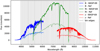 |
Fig. 1 Observed spectra of WASP-69 and reference star TYC 51871718-1 in the B (blue), RI (green), and z (red) grisms. Grey vertical lines indicate the edges of the spectroscopic light-curve bins. |
2.2 Simultaneous EulerCam photometry
In parallel with our VLT/FORS2 observations, we obtained broadband photometry with EulerCam (Lendl et al. 2012). Euler- Cam or ECAM is a 4k × 4k CCD camera installed at the 1.2 meter Euler telescope at La Silla, Chile. The observations were made with the Johnson-B filter (352–518 nm) to maximise the signal arising from any spot or facula crossings. In addition, taking simultaneous observations from la Silla and Paranal helps us to effectively disentangle weather- and instrument-related systematic effects from astrophysical signals.
3 Methods
3.1 Spectroscopy
We use a custom Python pipeline that we call HANSOLO (atmospHeric trANsmission SpectrOscopy anaLysis cOde), which was specially developed for the CHEWIE dataset to perform the data reduction and analysis of the FORS2 data. We analyse each night separately to obtain individual transmission spectra. Offsets between the transmission spectra of the different nights are corrected so that the B and z grism spectra align with the RI grism observations in the overlapping regions. The RI grism observations were chosen as a reference as it is the only mode with wavelength overlap with both the other modes. The spectra are then combined for a simultaneous stellar activity and atmospheric retrieval.
3.1.1 Spectral extraction and background removal
We followed the data reduction set out in Lendl et al. (2016, 2017) for FORS2 data. Standard bias and flatfield corrections were applied and the 2D detector images were wavelength calibrated using spectra taken with the ThAr lamps (performed with a mask identical to the science mask, but with 1″ slit widths).
Cosmic rays were identified during this step using the LACOS- MIC algorithm (van Dokkum 2001). The spectral extraction was performed on a column-by-column basis, with the middle of the trace being identified in each column by fitting a Moffat function. The background was removed by fitting a linear trend to 20 pixels at each edge of the slit and removing that from the column. The flux was then obtained by integrating over 11 apertures around the centre of the trace with widths of 25–75 pixels. We removed any outliers beyond 5–10 σ from the extracted spectra, depending on the quality of the data. These values were chosen to remove outliers from cosmic rays or broken pixels, without removing sections of the spectra with high levels of variation due to seeing or other observational factors. Overall, around 0.1% of the final data points were rejected. We aligned all spectra with the first observed spectrum by cross-correlating between three and five lines at different wavelengths depending on the availability of lines in the grism and fitted a second-order polynomial to the relative shifts. The spectra were then interpolated to fit the same wavelength grid. This accounts for both shifts and stretching of the trace on the detector due to varying observing conditions during the night. We then applied a second wavelength correction based on a PHOENIX model stellar spectrum with the same temperature and log(ɡ) as WASP-69.
3.1.2 White light curves
‘White’, that is, wavelength-integrated, light curves were obtained for the different apertures by integrating over the full spectra. The aperture with the lowest median absolute deviation (MAD) was selected for subsequent analysis. These correspond to apertures of 40, 70, and 65 pixels for the B, RI, and z grisms, respectively.
To obtain the system parameters, we first fitted the white light curves with a transit model and a Gaussian process (GP; Rasmussen & Williams 2006; Gibson et al. 2012; Gibson 2014) with a Matern 3/2 kernel using the CONAN transit fitting code (Lendl et al. 2017, 2020). We fixed the period and the eccentricity to the literature values (3.8681382±0.00000017 days and 0.00±0.05 respectively; Anderson et al. 2014) as we are analysing the different nights separately and so only have one transit per fit. We also fixed the limb-darkening parameters to values obtained with the LDCU code as they are highly degenerate with the impact parameter. LDCU2 is a modified version of the Python routine implemented by Espinoza & Jordán (2015) that computes the limb-darkening coefficients and their corresponding uncertainties using a set of stellar intensity profiles accounting for the uncertainties on the stellar parameters. In this case, the stellar parameters were obtained from Anderson et al. (2014): Teff = 4715 ± 50, log(ɡ) = 4.5 ± 0.15, and [Fe/H] = 0.114 ± 0.077. The stellar intensity profiles are generated based on two libraries of synthetic stellar spectra: ATLAS (Kurucz 1979) and PHOENIX (Husser et al. 2013). We adopted the Kipping parametrisation of the quadratic limb-darkening law for computational efficiency (Kipping 2013). The planet radius, the impact parameter, and the transit midpoint and duration are left as free parameters, as well as the GP hyperparameters. CONAN fits also include a flux offset, and a jitter parameter that estimates the extra white noise in the data. The full set of priors and the results for each night can be found in Table 2.
Figure 2 shows the white light curves in the upper panels, with the best fits overplotted in black. The middle panels show the residuals and the bottom panels show the residual after just the transit models have been removed, with the GP contributions to the models overplotted in black. As two of the curves contain signs of active-region crossing, we also fit the B and z grism white light curves with the data points around the crossings of active regions excluded, but find that the obtained parameters are not significantly different.
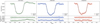 |
Fig. 2 FORS2 white light curves with noise models and residuals. The top row shows the white light curves and fits for all three nights: the first night observations were done in the RI grism (green, left), the second in the B grism (blue, middle), and the third in the z grism (red, right). Data points are indicated with open circles, while the solid lines indicate the fitted transit and GP model. The second row shows the residuals for each of the light curves and the third row shows the obtained common mode noise model in colour with the GP fit overplotted in black. The GP fits and common noise models for the B and z grisms clearly show the crossing of the respective active regions. |
White light fits for the three different nights.
3.1.3 Spectroscopic light curves
We also produced spectroscopic light curves by binning the spectra along the wavelength axis with a bin size of 10 nm, resulting in 27 light curves in the B grism, 34 light curves in the RI grism, and 33 light curves in the z grism.
We obtained a separate common noise model for each night by dividing the white light curve by the transit component of the fitted model. Because of this, the common noise model contains both correlated and uncorrelated noise contributions. The corresponding spectroscopic light curves were then divided by this model to remove any noise features common to all light curves. Both the original and detrended light curves are shown in Figs. A.2, A.3, and A.4, along with the common noise models for the B, RI, and z grism observations, respectively.
The spectroscopic light curves are fit with a combined transit and baseline model to account for any weather and instrumental effects still present in the data. For the transit model, the Mandel & Agol (2002) model is used. Only the planetary radius is fit, while the transit midpoint and duration and the impact parameter are fixed to the values obtained in the white light fits. Limbdarkening parameters are calculated for each bin to account for the change in limb darkening with wavelength, but are kept fixed as they are not well constrained when left free.
For the baseline model for each night, we tried various combinations of polynomials with time, airmass, spectrum full width at half maximum (FWHM), sky background, and trace position. More complicated models were only accepted over simpler models if the Bayesian information criterion (BIC) indicated a significantly higher probability (|ΔBIC| > 8). This resulted in a linear polynomial with the spectrum FWHM for all grisms and a polynomial with time that was second order in the B grism and first order in the RI and z grisms. These were chosen over another GP model to prevent overfitting after the removal of the common noise model. Instead, we estimate the residual white and red noise in the light curves by calculating the white and red noise factors for each light curve (βw and βr respectively; Winn et al. 2008; Gillon et al. 2010). βw is simply the root-mean-square (RMS) of the residuals over the mean of the errors, while βr compares the RMS of the binned photometric residuals to the RMS over the entire dataset. The errors of the photometric light curves are then inflated with CF = βw × βr and the light curves are fit again to obtain the error bars of the final spectrum. These fits and their residuals are plotted in the second and third columns of Figs. A.2, A.3, and A.4.
3.2 Atmospheric retrievals
To characterise the observations, we performed atmospheric retrieval calculations using the open-source Bern Atmospheric Retrieval code (BEAR)3. This code is an updated version of the retrieval code previously named HELIOS-R2 (Kitzmann et al. 2020). BEAR employs the MULTINEST (Feroz & Hobson 2008) library to perform the parameter space exploration using Bayesian nested sampling (Skilling 2004). The number of live sampling points was 4000 for all retrieval calculations performed in this study. In the present work, we used the transmission spectroscopy forward model of BEAR. It assumes an isothermal atmosphere with a temperature T and a surface gravity log ɡ. For this study, the atmosphere extended from a pressure of 10 bar at the bottom to 10−6 bar at the top and is divided into 100 atmospheric layers distributed equidistantly in logarithmic pressure space. The planet’s radius at the bottom of the atmosphere, Rp , was used as a free parameter.
The abundance profiles of the chemical species were assumed to be constant with pressure, described by a single mixing ratio xi per considered species. In the retrievals, we used the mixing ratios of water (H2O), titanium oxide (TiO), ammonia (NH3), sodium (Na), and potassium (K) as free parameters. While gaseous TiO might not be expected at the relatively cool equilibrium temperature of WASP-69b (Teq = 963 ± 18; Anderson et al. 2014), it is nevertheless included in the retrieval due to a potential detection of it by Ouyang et al. (2023). Other molecules, such as methane or hydrogen cyanide, were initially considered as well, but were unconstrained and were therefore removed from the retrieval calculations.
Opacity tables for H2O, TiO, and NH3 were computed by the open-source HELIOS-K4 code (Grimm & Heng 2015; Grimm et al. 2021) based on line-list data published by Polyansky et al. (2018), McKemmish et al. (2019), and Al Derzi et al. (2015), respectively. The opacities for K and Na are based on the Kurucz line list (Kurucz 2017), with additional data for the description of the resonance line wings based on the work by Allard et al. (2012), Allard et al. (2016), and Allard et al. (2019).
For this study, we added a stellar contamination module to BEAR, following the description by Rackham et al. (2018).
Thus, we modelled the transmission spectrum under the impact of stellar contamination due to spots and faculae according to
 (1)
(1)
where Dλ and Dλ,obs are the true and observed transit depths, ffac and fspot are the spot and faculae covering fractions, Fphot is the photospheric spectrum of the star, and Fspot and Ffac are the spectra of the spots and faculae, respectively. We sampled the corresponding spectra from the spectral library by Husser et al. (2013) based on the PHOENIX stellar atmosphere model. For a given set of stellar parameters, namely surface gravity log ɡ*, stellar effective temperature Teff,*, and metallicity [Fe/H], we performed a three-dimensional interpolation within the PHOENIX grid to obtain the stellar photospheric spectrum Fphot. The spectra for the spots and faculae were interpolated with the same surface gravity and metallicity but at different temperatures Tfac = Teff,* + ΔTfac and Tspot = Teff,* − ΔTspot, where ΔTfac and ΔTspot are used as free parameters in the retrieval.
Additionally, we also considered a cloud layer for our retrieval calculations. Previous studies by Fisher & Heng (2018), Murgas et al. (2020), Estrela et al. (2021), and Ouyang et al. (2023) suggested the presence of small aerosols in the atmosphere that cause an upward spectral slope in the optical wavelength range. We therefore included a new power-law cloud model in BEAR, where the optical depth as a function of wavelength follows a given power law. The (vertical) wavelengthdependent optical depth of the cloud layer is determined by the exponent of the power law ec and the optical depth at a reference wavelength τc:
 (2)
(2)
where λref is the reference wavelength for which we used a value of 1 μm. For a cloud layer that exhibits a Rayleigh scattering-like behaviour, for example, ec would be −4. The cloud’s location in the atmosphere is determined by a cloud-top pressure pc and its vertical extent is assumed to be one atmospheric scale height.
A full list of all priors and their corresponding distributions can be found in Table 3. We also tested retrievals with a grey cloud and a clear-sky atmosphere, respectively. The grey cloud model only has two free parameters, the cloud top pressure and the optical depth of the cloud layer.
3.3 Simultaneous EulerCam photometry
Using the standard aperture photometry pipeline for EulerCam as described in Lendl et al. (2012) to perform bias, flat, and overscan corrections, we obtained EulerCam light curves for each night of FORS2 observations. The aperture photometry is performed for different sets of circular apertures of varying size and different reference stars in the field of view. We selected our final light curves by minimising the photometric scatter between consecutive flux measurements; these are shown in Fig. A.1.
To account for any correlated noise arising from instrumental systematic uncertainties, weather, and so on, we fitted the observed light curves with a photometric baseline model along with the pure transit model. The optimal baseline is determined by iteratively fitting different baseline models involving air mass, exposure time, sky background, shifts, and the FWHM of stellar point spread function (PSF), minimising the BIC. For the first night, 18 July 2017, a combination of a second-order polynomial of the FWHM of the stellar PSF and a first-order polynomial of the exposure time is used. For the second night, 14 August 2017, a combination of a first-order polynomial of the air mass, a second-order polynomial of the FWHM of the stellar PSF, and a first-order polynomial of the sky background is used. Lastly, for the third night, 18 August 2017, a second-order polynomial of the air mass and a first-order polynomial of the exposure time are used.
Both the FORS2 and EulerCam light curves taken on the third night show signs of an active region crossing. To model the properties of the hot region, we used an adapted version of the PyTranSpot code, which is designed to model multi-band transit light curves showing starspot anomalies (Juvan et al. 2018; Chakraborty et al. 2024). We use blackbody radiation to model the emissions from the quiet photosphere and the facula. Since both light curves involve the same facula, we consider the contrast between the facula and the stellar surface in both wavelength bands to be related through a blackbody to the same temperature. This constraint on the contrast ratio between the two bands allows us to constrain the temperature, despite the degeneracy between contrast and surface area, which is usually present when fitting active region crossings. We further set the mid-transit time, transit depths, quadratic limb-darkening coefficients, location of the active region, size, and temperature as jump parameters and provided wide uniform priors for model optimisation. The full set of parameters, their priors, and the results can be found in Table 4.
Retrieval parameters and prior distributions used for the retrieval model.
4 Results
Despite being treated entirely separately, the impact parameter and transit durations obtained from the white light fits are identical during the nights the RI and z grism observations were taken and the B grism impact parameter is consistent within 1σ, while the transit duration is consistent within 2σ.
4.1 Transmission spectrum
The transmission spectra of all three observations are plotted in the top panel of Fig. 3. An offset is applied between the B and z grism observations to align them to the RI observations in the overlapping wavelength regions. This is common practice due to differences in systematic instrumental and weather effects between observations, as well as the effect of the common noise model removal. The final values of the planet radius can also be found in Tables A.1, A.2, and A.3. Error bars at the blue and red ends of the wavelength range are larger due to the reduced signal-to-noise ratio in the spectra in those regions, which is caused by lower grism throughput. This is especially the case for the bluest wavelength points, where the added lower efficiency of the MIT detector – used for all three observations – further increases the error bars. Because of this, we do not consider the uptick in apparent radius at the three shortest wavelength points to be significant.
Generally, the different nights are in good agreement in the overlapping regions. Both the RI and z grism observations show a relatively high transit depth at ∼7600 Å, but this coincides with the telluric oxygen band and is therefore unlikely to be a planetary feature.
The combined transmission spectrum does not show any obvious atomic or molecular features, indicating possible cloud cover, but it does show a clear decrease in the apparent planetary radius towards the blue that is characteristic of unocculted faculae.
Phase offset with respect to a mid-transit time of 2 457 984.62 BJD_TDB.
4.2 Atmospheric retrievals
The main feature of the transmission spectrum is the drop in apparent radius at the blue end, which indicates stellar activity contamination. The median of all posterior spectra for the power-law cloud retrieval is displayed in Fig. 3 in grey on top of the observational data. The posterior distributions for the stellar activity parameters are shown in the lower panel of Fig. B.1. We do not plot the posterior distributions for the star’s surface gravity and metallicity, because those are sampled from their Gaussian distributions listed in Table 3. However, the retrieval prefers a median stellar effective temperature slightly higher than that of its original Gaussian distribution. Our constraints on the temperature of the faculae suggest that they have a median temperature of about 5170±72 K, or roughly 230 K hotter than the fitted stellar effective temperature of 4939±55 K. With a median temperature of about 4618±110 K, the spots are around 320 K below the stellar effective temperature. The spot and facula coverage fractions are both near 30%.
Beyond the stellar contamination, the spectrum is missing any obvious features, including those of the alkali metals. As a result, our retrievals suggest the presence of a high-altitude cloud layer in the atmosphere, confirming the findings by, for example, Fisher & Heng (2018) and Estrela et al. (2021). The cloud layer is located at a very low pressure of about 1.4 mbar with a 1σ interval of 0.4–4 mbar. This very high-altitude cloud is necessary for the retrieval to explain the lack of strong molecular features in the transmission spectrum. In contrast to previous studies, we do not find evidence for a Rayleigh-like scattering haze. The power law index ec of our cloud model is mostly unconstrained; see the upper panel of Fig. B.1. This is caused by the strong impact of the stellar contamination at smaller wavelengths, which dominates any upward slope in the transmission spectrum that would be caused by small aerosol particles. We also note that while an upward slope in the transmission spectrum could be caused by small scattering cloud particles, it could also originate from stellar contamination with predominant spots.
In addition to the power-law cloud, we also performed an additional retrieval test with a grey cloud layer (not shown). This retrieval yields almost the same posterior distributions for the chemical species and atmospheric temperature, suggesting that a grey cloud is the most probable scenario to describe our observations of WASP-69b. The Bayesian evidence of the greycloud model (In 𝒵 = −613.663) is only marginally higher than that with the power-law cloud (In 𝒵 = −614.041). The preference for the grey-cloud model is caused by a reduced number of free parameters to explain the data. However, the Bayes factor between the two models is only 1.45 and, thus, the difference is statistically insignificant. The relative lack of constraint on the power-law index ec and the preference for a grey cloud also means that the cloud-particle size cannot be sufficiently constrained.
For comparison, we also performed a cloud-free retrieval. The corresponding posterior distributions can be found in Appendix B.2. The median model is included in the top panel of Fig. 3 in blue. Without a cloud layer, the abundances of essentially all chemical species shift by at least about an order of magnitude to lower values. Furthermore, the atmospheric temperature becomes prior-dominated at the lower prior boundary of 500 K. Thus, without the cloud layer, the retrieval aims to dampen the molecular features in the transmission spectrum by reducing the temperature, thereby making the atmospheric scale height smaller. The posteriors for the stellar contamination are, on the other hand, roughly similar to those for the cloudy models. The retrieved temperatures are consistent within their 1σ intervals. Only the posterior distribution for ffac is slightly more skewed in the cloud-free case, shifting its median value away from the maximum of the distribution. However, both fractional coverages ffac and fspot are still consistent with those of the cloudy retrieval calculations within their 1σ intervals. The cloud-free retrieval model has a substantially lower Bayesian evidence (In 𝒵 = −619.213). Compared to the power-law cloud model discussed above, the Bayes factor is about 176, suggesting that a cloudy model is strongly preferred over the clear-sky one.
For the favoured power-law cloud retrieval, our retrieved atmospheric temperature of  K is slightly cooler than the zero-albedo estimate on the equilibrium temperature of 963 ± 18 K reported by Anderson et al. (2014). The sodium feature is clearly suppressed due to the aforementioned clouds, which gives us a median mixing ratio of 10−9 with a relatively large uncertainty of nearly 2 dex. Additionally, the sodium feature lies in the overlapping region of the B and RI grism wavelengths, meaning there are two data points from different nights at the same wavelength. These points are consistent with each other, but the difference between them still introduces extra uncertainty in the retrieved sodium abundance, which leads to a very weak constraint. This is consistent with previous detections of sodium at high resolution, where the strong line core can be resolved (Casasayas-Barris et al. 2017; Deibert et al. 2019; Khalafinejad et al. 2021). The bottom panel of Fig. 3 shows that the contribution of sodium to the final spectrum is small compared to the contributions of the other molecules included in the retrieval. These contributions were obtained by postprocessing the posterior sample and selectively removing a specific absorber. The comparison with the median spectrum of the full posterior sample then yields the relative contribution of the removed species to the full model.
Similar to sodium, we also do not see a potassium feature. Instead, we find a 3σ upper limit on the potassium abundance of <10−7. Unlike sodium, potassium has not previously been detected in the atmosphere of WASP-69b (Deibert et al. 2019; Murgas et al. 2020). It is possible that this is at least in part due to the fact that the potassium feature coincides with a telluric oxygen absorption band. We also put an upper limit on the abundance of titanium oxide of <10−7.7 at 3σ significance. This means we cannot confirm the hints of TiO seen by Ouyang et al. (2023), who retrieved abundances of the order of 10−2.5.
We do constrain the abundances of water and ammonia, with median mixing ratios of about 0.01 and 10−3.4, respectively. These values are consistent with previous observations of water, including infrared data from HST (Tsiaras et al. 2018; Khalafinejad et al. 2021; Guilluy et al. 2022; Schlawin et al. 2024), and ammonia (Guilluy et al. 2022) in the atmosphere of WASP-69b. Tsiaras et al. (2018) do show a posterior for ammonia in their Fig. 4 that appears to indicate its presence, but this is not further expanded upon. The high abundances of both water and ammonia are driven by the rise in the red end of the transmission spectrum. Both molecules have opacities that increase towards the infrared and therefore make large contributions to the spectrum beyond 7000 Å. This can be seen in the bottom panel of Fig. 3, where the contributions to the transmission spectrum of water are plotted in blue and those of ammonia in yellow. Individual retrievals without water and without ammonia show that the molecules are somewhat degenerate, with neither being preferred over the retrieval with both (Bayesian evidences of 1.8 and 1.14 respectively). However, a retrieval without either molecule is not able to capture the rise and results in a Bayesian evidence of 3.5, equivalent to a detection of 2.2σ. Additionally, while the high abundance of NH3 in particular may seem surprising, recent theoretical non-equilibrium chemistry calculations for the atmospheric composition of the terminator region of WASP-69b (Bangera et al., in review) suggest that strong vertical mixing of ammonia increases its abundance considerably compared to a chemical-equilibrium case. The authors of this latter study obtained a mixing ratio of about 10−4 in the upper part of the atmosphere, which is consistent with our value within its 1σ interval.
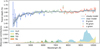 |
Fig. 3 Transmission spectrum of WASP-69b. Top: data points and retrieved models. The blue green and red points are the transit depths obtained from the B, RI, and z grism observations, respectively. The grey line represents the median of all retrieval posterior sample spectra for the favoured power-law cloud model, with the shaded region indicating their 1σ interval. The blue line represents the cloud free model. Bottom: relative contributions of the different atoms and molecules to the retrieved spectrum. |
4.3 Active region crossings
Two of the FORS2 white light curves show potential active region crossings. The B grism light curve shows a bump just before egress that is likely a spot crossing. However, the Euler- Cam data are of insufficient quality to confirm this, as the correlated noise is of the same amplitude as the potential spot crossing.
The z grism light curve shows a dip in flux just after ingress. This dip coincides with a change in exposure time due to weather circumstances, although we would expect the use of a reference star to diminish the resulting effects on the light curve. Added credibility is lent to the reality of this feature by the simultaneous EulerCam light curve, which shows a similar drop at the same location during transit. Even more so, the drop is slightly larger, as expected for a facula crossing observed in a bluer bandpass. Since the Euler telescope is located in La Silla and the VLT in Paranal, the atmospheric effects in both light curves are expected to be different and no change in exposure time was required until the egress of the transit, long after the flux drop. Because of this, we consider the drop to be due to the planet crossing a facula on the stellar surface, temporarily increasing the occulted flux.
The stellar surface model and the models for both light curves are shown in Fig. 4 and the results of the fit are presented in Table 4. We find the anomaly in the light curve to be best fit by the planet crossing a facula of  in diameter and with a temperature of
  K above the rest of the star.
5 Discussion
5.1 Stellar activity changes
The retrieved activity is dominated by the slope in the B grism part of the spectrum. As the data were taken over three separate nights, it is possible that the activity changed between observations.
The stellar rotation period is 23–24 days (Anderson et al. 2014; Khalafinejad et al. 2021). As the B and z grism observations are taken 4 days or one-sixth of a rotation apart and the star is inclined to a nearly pole-on orientation (~65º; Chakraborty et al. 2024, Allart et al., in prep.), only a small fraction of the surface is expected to have changed and we do not expect significant differences in activity between these observations, either from activity evolution or from the stellar rotation changing the visible part of the surface. The RI and B grism observations are taken 26 days apart, which is just over a full rotation. However, cooler stars are expected to have longer-lived active regions and Kepler observations of stars with 20 day rotation periods have shown active region lifetimes of 20–200 days for K stars with similar temperatures to WASP-69 (Giles et al. 2017). While it is possible that the activity evolved significantly between the RI and B grism observations, this is unlikely.
5.2 Unocculted activity features
Chakraborty et al. (2024) previously fitted a spot covering fraction of ~1% for WASP-69 using rotational modulation in the TESS (Transiting Exoplanet Survey Satellite) light curve, but this is a lower limit under the assumption that the star is viewed at exactly 90° inclination. The fact that the system is likely inclined means that there is a large area of the stellar surface that does not rotate out of view. Additional activity can therefore be present without changing the observed intensity variations, which is reflected in the lack of an upper limit on the spot size when fitting the TESS light curve with inclination as a free parameter. In this fit, the inclination comes out to 67±8°.
Three previous studies obtained medium-resolution transmission spectra of WASP-69 b and analysed possible activity. Murgas et al. (2020) observed WASP-69b with OSIRIS (Optical System for Imaging and low-Intermediate-Resolution Integrated Spectroscopy) on the GTC (Gran Telescopio Canarias) in 2016, a year before our own observations. Estrela et al. (2021) combined data from STIS (Space Telescope Imaging Spectrograph) and WFC3 (Wide Field Camera 3) on Hubble, taken in May and October of 2017, two months before and two months after our own observations. Finally, Ouyang et al. (2023) coincidentally observed the same night as our RI grism observations with the 4m SOAR telescope (SOuthern Astrophysical Research telescope). Their transmission spectrum shows a slope that is not present in ours. Of these three studies, only Estrela et al. (2021) have any data at shorter wavelengths than ≈500 nm, where the effect of unocculted faculae are stronger, and even then only to ≈450 nm. A combination of unocculted faculae and starspots could still introduce a positive slope into the spectrum at their observed wavelengths if the spot coverage fraction were higher than the facula coverage fraction. A difference of 10 percentagepoints between the two is enough to introduce a visible slope in the spectrum at the retrieved temperatures, with the slope increasing with the difference. Activity evolution could therefore explain the differences with both Murgas et al. (2020) and Estrela et al. (2021), despite the latter observations only being a few months apart. Finally, the Ouyang et al. (2023) observations were taken on the same night, but are still limited in the blue wavelength range, making detection of unocculted facula signatures impossible. Additionally, between 560 and 870 nm, our spectrum and that of Ouyang et al. (2023) are generally consistent within 1σ. It is only at the extreme ends of their spectrum that the differences arise, which coincide with an increase in the correlation of the residuals and in the size of the error bars. It is possible that the effects of differences in the treatment of correlated noise are especially apparent at these wavelengths, as wavelength-correlated noise can introduce a slope into the spectrum if it is not fully accounted for (Fortune et al. 2024). Additionally, the data from Estrela et al. (2021) were reanalysed by Allen et al. (2024). These latter authors found a different slope and concluded that they could not distinguish between planet atmosphere and stellar contamination with the precision available in the data. They did not provide any parameters for their stellar contamination model. An overview of the retrieved possible activity parameters of the first three works mentioned above is shown in Table 5.
Although all three studies found that their spectra could be fully explained by stellar activity contamination, the authors ultimately concluded that since no spot crossings had been observed, significant activity is unlikely; the authors therefore attributed all spectral features to the planet atmosphere.
Considering the obvious facular signal in our transmission spectrum, the facula crossing in one of our light curves, and the possible spot crossing in another, we do not come to the same conclusion.
It is worth noting that the obtained spot and facula coverage fractions and their temperatures are consistent across the four datasets, although this is in large part due to the difficulty of constraining these parameters, which leaves large error bars. We also find our retrieved parameters for the unocculted faculae to be consistent with the properties obtained from other low-resolution transmission spectra that show facular contamination. These studies find temperatures of 150–350 K (±~200K) hotter than the stellar surface and coverage fractions of 3–20% (±~20%) (Rackham et al. 2017; Kirk et al. 2021; Jiang et al. 2021; Nikolov et al. 2021; Cadieux et al. 2024).
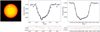 |
Fig. 4 PyTranSpot models for ECAM and FORS2 observations taken on 18 August 2017. Left: toy model of the stellar surface with the occulted facula and transit chord marked. Middle and right: detrended ECAM and FORS2 white light curves with the transit + facula model on top. |
Retrieved possible activity levels in previous studies compared to this work. Dashes indicate that parameters were not fitted for. Values with no error bars were held fixed.
5.3 Crossed facula temperatures
Previous works discussing facula crossings are relatively rare compared to works discussing spot crossings, but include five works discussing transits of single stars and one work that included a statistical analysis of 26 targets (Mohler-Fischer et al. 2013; Kirk et al. 2016; Zaleski et al. 2019, 2020; Jiang et al. 2021; Baluev et al. 2021). Of the five individually studied stars, three are K-type stars (HATS-2, WASP-52 and HAT-P-12; Mohler-Fischer et al. 2013; Kirk et al. 2016; Jiang et al. 2021) and the other two are a late G star (Kepler-71; Zaleski et al. 2019) and an early M-type star (Kepler-45; Zaleski et al. 2020), both of which are relatively close to K-type stars. Baluev et al. (2021) do not provide spot-occurrence rates as a function of stellar type. As WASP-69 is also a K-type star, this suggests there may be an underlying mechanism that makes K-type stars more likely to have bright regions on the surface. It is suggested that K- stars are typically spot-dominated (e.g. Solanki 1999; Meunier 2024), but faculae can still exist at the edges of the spots, where they can span large areas and last longer than their host spots (Chatzistergos et al. 2022).
Of the five works discussing individual systems, only Zaleski et al. (2019) provide a temperature for the faculae crossed by their planet, which is 200±150 K higher than that of the star for an active region of approximately the same size as the planet, which is consistent with the 130–350 K values from unocculted faculae, and similar to the values found for photospheric faculae on the Sun (100–500 K depending on the height in the photosphere; e.g. Fröhlich & Lean 2004; Buehler et al. 2015; Solov’ev & Kirichek 2019; Pietrow et al. 2020; Kuridze et al. 2024).
With a measured temperature difference of approximately 600 K, our facula temperature is higher than previous observations, but still consistent with solar values. It is also somewhat higher than the ~200 K obtained from our measurement of unocculted faculae on WASP-69. However, since that temperature is an average over all the unocculted activity, it is possible that the facula crossing happened to be of a relatively hot region. Additionally, our fit assumes a circular shape for the facula, which is not necessarily accurate given that these features tend to form in between granules (e.g. da Silva Santos et al. 2023; Danilovic 2023). An elongated shape in the direction perpendicular to the planets path would result in the same crossing time, but a lower contrast area. Increasing the surface area in this way by a factor of two while maintaining the total emission would be possible within the transit chord and would result in a temperature difference of approximately 300 K, which is consistent with all the above values within 1σ.
6 Conclusions
We obtained a ground-based transmission spectrum of WASP- 69 from 340 to 1100 nm by combining three transits observed in different filters with FORS2 on the VLT. We observe a clear drop in the transmission spectrum at blue wavelengths, which is a tell-tale sign of stellar contamination from faculae. We independently confirm this event through the detection of a facula-crossing event observed simultaneously with different facilities. We therefore conclude that even though previous studies dismissed stellar contamination due to a lack of spot crossings, the star is indeed active and this needs to be accounted for. We performed retrievals of combined stellar activity and planet atmosphere models and found spot and facula coverage fractions of approximately 30%. We also constrained the active region temperatures to 4618 ± 110 for spots and 5170 ± 72 for faculae, compared to 4939 ± 55 for the quiet surface, or −321 and +231 K, respectively. The planetary contribution is best described by high-altitude cloud deck, which largely suppresses molecular features. Because of this, we do not constrain the sodium abundance, but we do find indications of the presence of NH3 and H2O and are able to put upper limits on the abundances of TiO and K.
We also obtained simultaneous photometric monitoring data from ECAM on the Euler telescope and detected a facula crossing in both the FORS2 and ECAM data of the third night. This allowed us to break the contrast–area degeneracy and obtain a temperature of  K above the stellar effective temperature; although this value could be lower for an irregularly shaped facula rather than a circular one.
Data availability
Tables of the light curves are available at the CDS via anonymous ftp to cdsarc.cds.unistra.fr (130.79.128.5) or via https://cdsarc.cds.unistra.fr/viz-bin/cat/J/A+A/692/A83
Acknowledgements
This project has received funding from the European Research Council (ERC) under the European Union’s Horizon 2020 research and innovation programme (project FOUR ACES; grant agreement No 724427). It has also been carried out in the frame of the National Centre for Competence in Research PlanetS supported by the Swiss National Science Foundation (SNSF). D.Eh. and A.De. acknowledge financial support from the SNSF for project 200021_200726. It has also been carried out in the frame of the National Centre for Competence in Research PlanetS supported by the Swiss National Science Foundation (SNSF). A.P. is supported by the European Research Council (ERC) under the European Union’s Horizon 2020 research and innovationprogramme (grant agreement No. 833251 PROMINENT ERC-ADG 2018). D.E. acknowledges financial support from the SNSF for project 200021_200726. This project has been carried out within the framework of the NCCR PlanetS supported by the Swiss National Science Foundation under grants 51NF40_182901 and 51NF40_205606. We acknowledge support of the Swiss National Science Foundation under grant number PCEFP2_194576. P.E.C. was funded by the Austrian Science Fund (FWF) Erwin Schroedinger Fellowship, program J4595-N.
Appendix A Additional light curves
A.1 Euler light curves
Figure A.1 shows the light curves obtained with Euler during the simultaneous observations with FORS2. Due to the smaller size of the telescope, the quality of the data is less than that taken with FORS2, so the light curves of the first and second night are not used in further analysis.
All three light curves show significant correlated noise and scatter. The light curve of the first night shows a significant drop in flux just before the transit midpoint, which is due to an increase in atmospheric turbulence. The scatter in the light curve of the second night is too large to confirm or rule out the potential spot crossing observed in the FORS2 data observed on the same night. The light curve of the third night also shows a drop just before the transit midpoint, although a shorter one than the first night and one not caused by weather conditions. Instead, it coincides with the potential facula-crossing in the corresponding FORS2 light curve. Further analysis of this feature in both light curves is provided in Sect. 3.3. The results and discussion can be found in Sects. 4.3 and 5.3, respectively.
A.2 Spectroscopic light curves
Figures A.2, A.3, and A.4 show the spectroscopic binned light curves for the B, RI and z grisms. All light curves are binned to 10 nm along the wavelength axis. The left columns show the raw, uncorrected light curves, arranged from shortest wavelengths at the top to longest at the bottom of the plot, with the common noise model plotted in black at the very bottom. The middle columns show the corrected light curves with the fitted transit and baseline model overplotted in the same colour. Finally, the rightmost columns show the residuals for each light curve.
While some structure remains in some of the residuals these are accounted for in the red and white noise factors used to inflate the errorbars before the final fit of the light curves. The scatter in the light curves is the largest for the bluest B grism light curves and the reddest z grism light curves, where the spectral intensity is lowest. Additionally, there are two light curves at 7693 Å and 7893 Å in the RI grism where the scatter increases after the correction. These light curves correspond to the telluric oxygen feature.
The fitted transit depths for the light curves of all three nights are given in Tables A.1, A.2 and A.3.
Spectroscopic fit results for the B grism. The first column contains the wavelength of the binned light curve, the second the fitted planetary radii in units of the stellar radius.
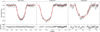 |
Fig. A.1 Detrended EulerCam light curves observed simultaneously to the FORS2 data. From left to right, the light curves of the first, second and third night. The top panel show the data after detrending and the transit fit, the bottom panels show the residuals. |
Spectroscopic fit results for the RI grism. The first column contains the wavelength of the binned light curve, the second the fitted planetary radii in units of the stellar radius.
Spectroscopic fit results for the z grism. The first column contains the wavelength of the binned light curve, the second the fitted planetary radii in units of the stellar radius.
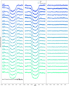 |
Fig. A.2 Spectroscopic light curves observed on 15 August 2017 in the B grism. The raw light curves are plotted in the left panel in color, with the shortest wavelengths at the top (bluest) and the longest at the bottom (greenest). The common mode as determined from the white light curve is plotted at the bottom in black. The light curves with the common mode removed are plotted in the middle panel with the fitted transits overplotted in the same color. The residuals are shown in the right panel. |
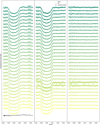 |
Fig. A.3 Spectroscopic light curves observed on 19 July 2017 in the RI grism. The raw light curves are plotted in the left panel in color, with the shortest wavelengths at the top (greenest) and the longest wavelengths at the bottom (yellowest). The common mode as determined from the white light curve is plotted at the bottom in black. The light curves with the common mode removed are plotted in the middle panel with the fitted transits overplotted in the same color. The residuals are shown in the right panel. |
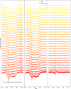 |
Fig. A.4 Spectroscopic light curves observed on 19 August 2017 in the z grism. The raw light curves are plotted in the left panel in color, with the shortest wavelengths at the top (yellowest) and the longest wavelengths at the bottom (reddest). The common mode as determined from the white light curve is plotted at the bottom in black. The light curves with the common mode removed are plotted in the middle panel with the fitted transits overplotted in the same color. The residuals are shown in the right panel. |
Appendix B Retrievals
B.1 Main retrieval
Figure B.1 shows the posteriors of the main atmospheric and stellar retrieval discussed in Sect. 4.2. The resulting spectrum is shown in Fig. 3.
B.2 Cloud-free atmospheric retrieval
A retrieval with a cloud-free planetary atmosphere was run for comparison with the cloudy scenario. The posteriors for this scenario are shown in Fig. B.2. Similar to the cloudy case, the posteriors for the surface gravity and metallicity are not shown, since they are essentially sampled from the Gaussian distributions. The resulting spectrum is shown in Fig. 3.
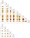 |
Fig. B.1 Posterior distributions for the planet’s atmosphere properties (top) and the stellar parameters (bottom). The vertical, magenta lines in the histogram plots refer to the median value of the depicted distribution, while the blue, vertical lines denote the 1 σ intervals. The three contour lines in the two-dimensional correlation plots refer to the 1 σ, 2σ, and 3σ regions, respectively. |
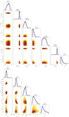 |
Fig. B.2 Posterior distributions for the planet’s atmosphere properties (top) and the stellar parameters (bottom) for the cloud-free retrieval model. The vertical, magenta lines in the histogram plots refer to the median value of the depicted distribution, while the blue, vertical lines denote the 1 σ intervals. The three contour lines in the two-dimensional correlation plots refer to the 1 σ, 2σ, and 3σ regions, respectively. |
References
- Al Derzi, A. R., Furtenbacher, T., Tennyson, J., Yurchenko, S. N., & Császár, A. G. 2015, J. Quant. Spectrosc. Radiat. Transf., 161, 117 [NASA ADS] [CrossRef] [Google Scholar]
- Allard, N. F., Kielkopf, J. F., Spiegelman, F., Tinetti, G., & Beaulieu, J. P. 2012, A&A, 543, A159 [NASA ADS] [CrossRef] [EDP Sciences] [Google Scholar]
- Allard, N. F., Spiegelman, F., & Kielkopf, J. F. 2016, A&A, 589, A21 [NASA ADS] [CrossRef] [EDP Sciences] [Google Scholar]
- Allard, N. F., Spiegelman, F., Leininger, T., & Molliere, P. 2019, A&A, 628, A120 [NASA ADS] [CrossRef] [EDP Sciences] [Google Scholar]
- Allen, N. H., Sing, D. K., Espinoza, N., et al. 2024, AJ, submitted [arXiv:2405.20361] [Google Scholar]
- Anderson, D. R., Collier Cameron, A., Delrez, L., et al. 2014, MNRAS, 445, 1114 [NASA ADS] [CrossRef] [Google Scholar]
- Appenzeller, I., Fricke, K., Fürtig, W., et al. 1998, The Messenger, 94, 1 [NASA ADS] [Google Scholar]
- Baluev, R. V., Sokov, E. N., Sokova, I. A., et al. 2021, Acta Astron., 71, 25 [NASA ADS] [Google Scholar]
- Bruno, G., Lewis, N. K., Stevenson, K. B., et al. 2018, AJ, 156, 124 [NASA ADS] [CrossRef] [Google Scholar]
- Buehler, D., Lagg, A., Solanki, S. K., & van Noort, M. 2015, A&A, 576, A27 [NASA ADS] [CrossRef] [EDP Sciences] [Google Scholar]
- Buehler, D., Lagg, A., van Noort, M., & Solanki, S. K. 2019, A&A, 630, A86 [NASA ADS] [CrossRef] [EDP Sciences] [Google Scholar]
- Cadieux, C., Plotnykov, M., Doyon, R., et al. 2024, ApJ, 960, L3 [NASA ADS] [CrossRef] [Google Scholar]
- Carter, A. L., Nikolov, N., Sing, D. K., et al. 2020, MNRAS, 494, 5449 [NASA ADS] [CrossRef] [Google Scholar]
- Casasayas-Barris, N., Palle, E., Nowak, G., et al. 2017, A&A, 608, A135 [NASA ADS] [CrossRef] [EDP Sciences] [Google Scholar]
- Chakraborty, H., Lendl, M., Akinsanmi, B., Petit dit de la Roche, D. J. M., & Deline, A. 2024, A&A, 685, A173 [NASA ADS] [CrossRef] [EDP Sciences] [Google Scholar]
- Charbonneau, D., Brown, T. M., Noyes, R. W., & Gilliland, R. L. 2002, ApJ, 568, 377 [Google Scholar]
- Chatzistergos, T., Ermolli, I., Krivova, N. A., et al. 2022, A&A, 667, A167 [NASA ADS] [CrossRef] [EDP Sciences] [Google Scholar]
- Chintzoglou, G., De Pontieu, B., Martínez-Sykora, J., et al. 2021, ApJ, 906, 82 [CrossRef] [Google Scholar]
- Cretignier, M., Pietrow, A. G. M., & Aigrain, S. 2024, MNRAS, 527, 2940 [Google Scholar]
- Czesla, S., Huber, K. F., Wolter, U., Schröter, S., & Schmitt, J. H. M. M. 2009, A&A, 505, 1277 [NASA ADS] [CrossRef] [EDP Sciences] [Google Scholar]
- Danilovic, S. 2023, Adv. Space Res., 71, 1939 [NASA ADS] [CrossRef] [Google Scholar]
- da Silva Santos, J. M., Reardon, K., Cauzzi, G., et al. 2023, ApJ, 954, L35 [NASA ADS] [CrossRef] [Google Scholar]
- Deibert, E. K., de Mooij, E. J. W., Jayawardhana, R., et al. 2019, AJ, 157, 58 [NASA ADS] [CrossRef] [Google Scholar]
- Deming, D., Wilkins, A., McCullough, P., et al. 2013, ApJ, 774, 95 [Google Scholar]
- Dineva, E., Pearson, J., Ilyin, I., et al. 2022, Astron. Nachr., 343, e23996 [NASA ADS] [CrossRef] [Google Scholar]
- Espinoza, N., & Jordán, A. 2015, MNRAS, 450, 1879 [Google Scholar]
- Estrela, R., Swain, M. R., Roudier, G. M., et al. 2021, AJ, 162, 91 [NASA ADS] [CrossRef] [Google Scholar]
- Feroz, F., & Hobson, M. P. 2008, MNRAS, 384, 449 [NASA ADS] [CrossRef] [Google Scholar]
- Fisher, C., & Heng, K. 2018, MNRAS, 481, 4698 [Google Scholar]
- Fortune, M., Gibson, N. P., Foreman-Mackey, D., et al. 2024, A&A, 686, A89 [NASA ADS] [CrossRef] [EDP Sciences] [Google Scholar]
- Fröhlich, C., & Lean, J. 2004, A&A Rev., 12, 273 [CrossRef] [Google Scholar]
- Gao, P., Thorngren, D. P., Lee, E. K. H., et al. 2020, Nat. Astron., 4, 951 [NASA ADS] [CrossRef] [Google Scholar]
- Gibson, N. P. 2014, MNRAS, 445, 3401 [NASA ADS] [CrossRef] [Google Scholar]
- Gibson, N. P., Aigrain, S., Roberts, S., et al. 2012, MNRAS, 419, 2683 [NASA ADS] [CrossRef] [Google Scholar]
- Giles, H. A. C., Collier Cameron, A., & Haywood, R. D. 2017, MNRAS, 472, 1618 [Google Scholar]
- Gillon, M., Lanotte, A. A., Barman, T., et al. 2010, A&A, 511, A3 [NASA ADS] [CrossRef] [EDP Sciences] [Google Scholar]
- Grimm, S. L., & Heng, K. 2015, ApJ, 808, 182 [NASA ADS] [CrossRef] [Google Scholar]
- Grimm, S. L., Malik, M., Kitzmann, D., et al. 2021, ApJS, 253, 30 [NASA ADS] [CrossRef] [Google Scholar]
- Guilluy, G., Andretta, V., Borsa, F., et al. 2020, A&A, 639, A49 [EDP Sciences] [Google Scholar]
- Guilluy, G., Giacobbe, P., Carleo, I., et al. 2022, A&A, 665, A104 [NASA ADS] [CrossRef] [EDP Sciences] [Google Scholar]
- Guilluy, G., D’Arpa, M. C., Bonomo, A. S., et al. 2024, A&A, 686, A83 [NASA ADS] [CrossRef] [EDP Sciences] [Google Scholar]
- Husser, T.-O., Wende-von Berg, S., Dreizler, S., et al. 2013, A&A, 553, A6 [NASA ADS] [CrossRef] [EDP Sciences] [Google Scholar]
- Ioannidis, P., Huber, K. F., & Schmitt, J. H. M. M. 2016, A&A, 585, A72 [NASA ADS] [CrossRef] [EDP Sciences] [Google Scholar]
- Jiang, C., Chen, G., Pallé, E., et al. 2021, A&A, 656, A114 [NASA ADS] [CrossRef] [EDP Sciences] [Google Scholar]
- Juvan, I. G., Lendl, M., Cubillos, P. E., et al. 2018, A&A, 610, A15 [NASA ADS] [CrossRef] [EDP Sciences] [Google Scholar]
- Khalafinejad, S., Molaverdikhani, K., Blecic, J., et al. 2021, A&A, 656, A142 [NASA ADS] [CrossRef] [EDP Sciences] [Google Scholar]
- Kipping, D. M. 2013, MNRAS, 435, 2152 [Google Scholar]
- Kirk, J., Wheatley, P. J., Louden, T., et al. 2016, MNRAS, 463, 2922 [NASA ADS] [CrossRef] [Google Scholar]
- Kirk, J., Rackham, B. V., MacDonald, R. J., et al. 2021, AJ, 162, 34 [NASA ADS] [CrossRef] [Google Scholar]
- Kitzmann, D., Heng, K., Oreshenko, M., et al. 2020, ApJ, 890, 174 [Google Scholar]
- Kuridze, D., Uitenbroek, H., Wöger, F., et al. 2024, ApJ, 965, 15 [NASA ADS] [CrossRef] [Google Scholar]
- Kurucz, R. L. 1979, ApJS, 40, 1 [NASA ADS] [CrossRef] [Google Scholar]
- Kurucz, R. L. 2017, Canadian J. Phys., 95, 825 [NASA ADS] [CrossRef] [Google Scholar]
- Lecavelier Des Etangs, A., Pont, F., Vidal-Madjar, A., & Sing, D. 2008, A&A, 481, L83 [NASA ADS] [CrossRef] [Google Scholar]
- Lendl, M., Anderson, D. R., Collier-Cameron, A., et al. 2012, A&A, 544, A72 [NASA ADS] [CrossRef] [EDP Sciences] [Google Scholar]
- Lendl, M., Delrez, L., Gillon, M., et al. 2016, A&A, 587, A67 [NASA ADS] [CrossRef] [EDP Sciences] [Google Scholar]
- Lendl, M., Cubillos, P. E., Hagelberg, J., et al. 2017, A&A, 606, A18 [NASA ADS] [CrossRef] [EDP Sciences] [Google Scholar]
- Lendl, M., Bouchy, F., Gill, S., et al. 2020, MNRAS, 492, 1761 [NASA ADS] [CrossRef] [Google Scholar]
- Libby-Roberts, J. E., Schutte, M., Hebb, L., et al. 2023, AJ, 165, 249 [NASA ADS] [CrossRef] [Google Scholar]
- Mallia, E. A., Blackwell, D. E., & Petford, A. D. 1970, Nature, 226, 735 [CrossRef] [Google Scholar]
- Mandel, K., & Agol, E. 2002, ApJ, 580, L171 [Google Scholar]
- McCullough, P. R., Crouzet, N., Deming, D., & Madhusudhan, N. 2014, ApJ, 791, 55 [NASA ADS] [CrossRef] [Google Scholar]
- McKemmish, L. K., Masseron, T., Hoeijmakers, H. J., et al. 2019, MNRAS, 488, 2836 [Google Scholar]
- Meunier, N. 2024, Comp. Rendus Phys., 24, 140 [NASA ADS] [Google Scholar]
- Mohler-Fischer, M., Mancini, L., Hartman, J. D., et al. 2013, A&A, 558, A55 [NASA ADS] [CrossRef] [EDP Sciences] [Google Scholar]
- Montet, B. T., Tovar, G., & Foreman-Mackey, D. 2017, ApJ, 851, 116 [Google Scholar]
- Moran, S. E., Stevenson, K. B., Sing, D. K., et al. 2023, ApJ, 948, L11 [NASA ADS] [CrossRef] [Google Scholar]
- Murgas, F., Chen, G., Nortmann, L., Palle, E., & Nowak, G. 2020, A&A, 641, A158 [NASA ADS] [CrossRef] [EDP Sciences] [Google Scholar]
- Nielsen, M. B., Gizon, L., Schunker, H., & Karoff, C. 2013, A&A, 557, L10 [NASA ADS] [CrossRef] [EDP Sciences] [Google Scholar]
- Nikolov, N., Sing, D. K., Gibson, N. P., et al. 2016, ApJ, 832, 191 [NASA ADS] [CrossRef] [Google Scholar]
- Nikolov, N., Sing, D. K., Fortney, J. J., et al. 2018, Nature, 557, 526 [CrossRef] [Google Scholar]
- Nikolov, N., Maciejewski, G., Constantinou, S., et al. 2021, AJ, 162, 88 [NASA ADS] [CrossRef] [Google Scholar]
- Nortmann, L., Pallé, E., Salz, M., et al. 2018, Science, 362, 1388 [Google Scholar]
- Nutzman, P. A., Fabrycky, D. C., & Fortney, J. J. 2011, ApJ, 740, L10 [NASA ADS] [CrossRef] [Google Scholar]
- Oshagh, M., Boisse, I., Boué, G., et al. 2013, A&A, 549, A35 [NASA ADS] [CrossRef] [EDP Sciences] [Google Scholar]
- Oshagh, M., Santos, N. C., Ehrenreich, D., et al. 2014, A&A, 568, A99 [NASA ADS] [CrossRef] [EDP Sciences] [Google Scholar]
- Ouyang, Q., Wang, W., Zhai, M., et al. 2023, MNRAS, 521, 5860 [NASA ADS] [CrossRef] [Google Scholar]
- Pietrow, A. G. M., Kiselman, D., de la Cruz Rodríguez, J., et al. 2020, A&A, 644, A43 [NASA ADS] [CrossRef] [EDP Sciences] [Google Scholar]
- Polyansky, O. L., Kyuberis, A. A., Zobov, N. F., et al. 2018, MNRAS, 480, 2597 [NASA ADS] [CrossRef] [Google Scholar]
- Pont, F., Knutson, H., Gilliland, R. L., Moutou, C., & Charbonneau, D. 2008, MNRAS, 385, 109 [Google Scholar]
- Pont, F., Sing, D. K., Gibson, N. P., et al. 2013, MNRAS, 432, 2917 [NASA ADS] [CrossRef] [Google Scholar]
- Rackham, B., Espinoza, N., Apai, D., et al. 2017, ApJ, 834, 151 [Google Scholar]
- Rackham, B. V., Apai, D., & Giampapa, M. S. 2018, ApJ, 853, 122 [Google Scholar]
- Rasmussen, C. E., & Williams, C. K. I. 2006, Gaussian Processes for Machine Learning, 2nd edn. (Cambridge: MIT press), 79 [Google Scholar]
- Reinhold, T., Shapiro, A. I., Solanki, S. K., & Basri, G. 2023, A&A, 678, A24 [NASA ADS] [CrossRef] [EDP Sciences] [Google Scholar]
- Schlawin, E., Mukherjee, S., Ohno, K., et al. 2024, AJ, 168, 104 [NASA ADS] [CrossRef] [Google Scholar]
- Sedaghati, E., Boffin, H. M. J., MacDonald, R. J., et al. 2017, Nature, 549, 238 [Google Scholar]
- Silva, A. V. R. 2003, ApJ, 585, L147 [Google Scholar]
- Sing, D. K., Fortney, J. J., Nikolov, N., et al. 2016, Nature, 529, 59 [Google Scholar]
- Skilling, J. 2004, AIP Conf. Ser., 735, 395 [Google Scholar]
- Solanki, S. K. 1999, ASP Conf. Ser., 158, 109 [NASA ADS] [Google Scholar]
- Solanki, S. K. 2003, A&A Rev., 11, 153 [NASA ADS] [CrossRef] [Google Scholar]
- Solov’ev, A. A., & Kirichek, E. A. 2019, MNRAS, 482, 5290 [CrossRef] [Google Scholar]
- Spyratos, P., Nikolov, N., Southworth, J., et al. 2021, MNRAS, 506, 2853 [NASA ADS] [CrossRef] [Google Scholar]
- Tsiaras, A., Waldmann, I. P., Zingales, T., et al. 2018, AJ, 155, 156 [NASA ADS] [CrossRef] [Google Scholar]
- Tyler, D., Petigura, E. A., Oklopčić, A., & David, T. J. 2024, ApJ, 960, 123 [NASA ADS] [CrossRef] [Google Scholar]
- van Dokkum, P. G. 2001, PASP, 113, 1420 [Google Scholar]
- Vissapragada, S., Knutson, H. A., Jovanovic, N., et al. 2020, AJ, 159, 278 [Google Scholar]
- Wallack, N. L., Knutson, H. A., Morley, C. V., et al. 2019, AJ, 158, 217 [NASA ADS] [CrossRef] [Google Scholar]
- Winn, J. N., Holman, M. J., Torres, G., et al. 2008, ApJ, 683, 1076 [Google Scholar]
- Zaleski, S. M., Valio, A., Marsden, S. C., & Carter, B. D. 2019, MNRAS, 484, 618 [NASA ADS] [CrossRef] [Google Scholar]
- Zaleski, S. M., Valio, A., Carter, B. D., & Marsden, S. C. 2020, MNRAS, 492, 5141 [NASA ADS] [CrossRef] [Google Scholar]
BEAR is available in the GitHub repository: https://github.com/newstrangeworlds/bear
BEAR is available in the GitHub repository: https://github.com/newstrangeworlds/bear
HELIOS-K is available in the GitHub repository https://github.com/exoclime/HELIOS-K. The computed opacities can be downloaded from the DACE platform https://dace.unige.ch
All Tables
Retrieved possible activity levels in previous studies compared to this work. Dashes indicate that parameters were not fitted for. Values with no error bars were held fixed.
Spectroscopic fit results for the B grism. The first column contains the wavelength of the binned light curve, the second the fitted planetary radii in units of the stellar radius.
Spectroscopic fit results for the RI grism. The first column contains the wavelength of the binned light curve, the second the fitted planetary radii in units of the stellar radius.
Spectroscopic fit results for the z grism. The first column contains the wavelength of the binned light curve, the second the fitted planetary radii in units of the stellar radius.
All Figures
|
Fig. 1 Observed spectra of WASP-69 and reference star TYC 51871718-1 in the B (blue), RI (green), and z (red) grisms. Grey vertical lines indicate the edges of the spectroscopic light-curve bins. |
| In the text | |
|
Fig. 2 FORS2 white light curves with noise models and residuals. The top row shows the white light curves and fits for all three nights: the first night observations were done in the RI grism (green, left), the second in the B grism (blue, middle), and the third in the z grism (red, right). Data points are indicated with open circles, while the solid lines indicate the fitted transit and GP model. The second row shows the residuals for each of the light curves and the third row shows the obtained common mode noise model in colour with the GP fit overplotted in black. The GP fits and common noise models for the B and z grisms clearly show the crossing of the respective active regions. |
| In the text | |
|
Fig. 3 Transmission spectrum of WASP-69b. Top: data points and retrieved models. The blue green and red points are the transit depths obtained from the B, RI, and z grism observations, respectively. The grey line represents the median of all retrieval posterior sample spectra for the favoured power-law cloud model, with the shaded region indicating their 1σ interval. The blue line represents the cloud free model. Bottom: relative contributions of the different atoms and molecules to the retrieved spectrum. |
| In the text | |
|
Fig. 4 PyTranSpot models for ECAM and FORS2 observations taken on 18 August 2017. Left: toy model of the stellar surface with the occulted facula and transit chord marked. Middle and right: detrended ECAM and FORS2 white light curves with the transit + facula model on top. |
| In the text | |
|
Fig. A.1 Detrended EulerCam light curves observed simultaneously to the FORS2 data. From left to right, the light curves of the first, second and third night. The top panel show the data after detrending and the transit fit, the bottom panels show the residuals. |
| In the text | |
|
Fig. A.2 Spectroscopic light curves observed on 15 August 2017 in the B grism. The raw light curves are plotted in the left panel in color, with the shortest wavelengths at the top (bluest) and the longest at the bottom (greenest). The common mode as determined from the white light curve is plotted at the bottom in black. The light curves with the common mode removed are plotted in the middle panel with the fitted transits overplotted in the same color. The residuals are shown in the right panel. |
| In the text | |
|
Fig. A.3 Spectroscopic light curves observed on 19 July 2017 in the RI grism. The raw light curves are plotted in the left panel in color, with the shortest wavelengths at the top (greenest) and the longest wavelengths at the bottom (yellowest). The common mode as determined from the white light curve is plotted at the bottom in black. The light curves with the common mode removed are plotted in the middle panel with the fitted transits overplotted in the same color. The residuals are shown in the right panel. |
| In the text | |
|
Fig. A.4 Spectroscopic light curves observed on 19 August 2017 in the z grism. The raw light curves are plotted in the left panel in color, with the shortest wavelengths at the top (yellowest) and the longest wavelengths at the bottom (reddest). The common mode as determined from the white light curve is plotted at the bottom in black. The light curves with the common mode removed are plotted in the middle panel with the fitted transits overplotted in the same color. The residuals are shown in the right panel. |
| In the text | |
|
Fig. B.1 Posterior distributions for the planet’s atmosphere properties (top) and the stellar parameters (bottom). The vertical, magenta lines in the histogram plots refer to the median value of the depicted distribution, while the blue, vertical lines denote the 1 σ intervals. The three contour lines in the two-dimensional correlation plots refer to the 1 σ, 2σ, and 3σ regions, respectively. |
| In the text | |
|
Fig. B.2 Posterior distributions for the planet’s atmosphere properties (top) and the stellar parameters (bottom) for the cloud-free retrieval model. The vertical, magenta lines in the histogram plots refer to the median value of the depicted distribution, while the blue, vertical lines denote the 1 σ intervals. The three contour lines in the two-dimensional correlation plots refer to the 1 σ, 2σ, and 3σ regions, respectively. |
| In the text | |
Current usage metrics show cumulative count of Article Views (full-text article views including HTML views, PDF and ePub downloads, according to the available data) and Abstracts Views on Vision4Press platform.
Data correspond to usage on the plateform after 2015. The current usage metrics is available 48-96 hours after online publication and is updated daily on week days.
Initial download of the metrics may take a while.