| Issue |
A&A
Volume 593, September 2016
|
|
|---|---|---|
| Article Number | A22 | |
| Number of page(s) | 23 | |
| Section | Extragalactic astronomy | |
| DOI | https://doi.org/10.1051/0004-6361/201628249 | |
| Published online | 30 August 2016 | |
Size evolution of star-forming galaxies with 2 <z < 4.5 in the VIMOS Ultra-Deep Survey⋆
1 Aix Marseille Université, CNRS, LAM
(Laboratoire d’Astrophysique de Marseille) UMR 7326, 13388 Marseille, France
e-mail: This email address is being protected from spambots. You need JavaScript enabled to view it.
2 Instituto de Fisica y Astronomía,
Facultad de Ciencias, Universidad de Valparaíso, Gran Bretaña
1111, Playa Ancha, Valparaíso, Chile
3 INAF–IASF Milano, via Bassini 15,
20133
Milano,
Italy
4 INAF–Osservatorio Astronomico di
Bologna, via Ranzani, 40127
Bologna,
Italy
5 INAF–Osservatorio Astronomico di
Roma, via di Frascati 33, 00040
Monte Porzio Catone,
Italy
6 Astronomy Department, University of
Massachusetts, Amherst, MA
01003,
USA
7 Space Telescope Science Institute,
3700 San Martin
Drive, Baltimore,
MD
21218,
USA
8 SUPA, Institute for Astronomy,
University of Edinburgh, Royal Observatory, Edinburgh, EH9 3HJ, UK
Received:
2
February
2016
Accepted:
22
June
2016
Abstract
Context. The size of a galaxy encapsulates the signature of the different physical processes driving its evolution. The distribution of galaxy sizes in the Universe as a function of cosmic time is therefore a key to understand galaxy evolution.
Aims. We aim to measure the average sizes and size distributions of galaxies as they are assembling before the peak in the comoving star formation rate density of the Universe to better understand the evolution of galaxies across cosmic time.
Methods. We used a sample of ~1200 galaxies in the COSMOS and ECDFS fields with confirmed spectroscopic redshifts 2 ≤ zspec ≤ 4.5 in the VIMOS Ultra Deep Survey (VUDS), representative of star-forming galaxies with iAB ≤ 25. We first derived galaxy sizes by applying a classical parametric profile-fitting method using GALFIT. We then measured the total pixel area covered by a galaxy above a given surface brightness threshold, which overcomes the difficulty of measuring sizes of galaxies with irregular shapes. We then compared the results obtained for the equivalent circularized radius enclosing 100% of the measured galaxy light r100T ~2.2 to those obtained with the effective radius re,circ measured with GALFIT.
Results. We find that the sizes of galaxies computed with our non-parametric approach span a wide range but remain roughly constant on average with a median value r100T ~2.2 kpc for galaxies with 2 <z< 4.5. This is in stark contrast with the strong downward evolution of re with increasing redshift, down to sizes of <1 kpc at z ~ 4.5. We analyze the difference and find that parametric fitting of complex, asymmetric, multicomponent galaxies is severely underestimating their sizes. By comparing r100T with physical parameters obtained through fitting the spectral energy distribution we find that the star-forming galaxies that are the largest at any redshift are, on average, more massive and form more stars. We discover that galaxies present more concentrated light profiles with increasing redshifts. We interpret these results as the signature of several, possibly different, evolutionary paths of galaxies in their early stages of assembly, including major and minor merging or star formation in multiple bright regions.
Key words: galaxies: high-redshift / galaxies: evolution / galaxies: structure
Based on data obtained with the European Southern Observatory Very Large Telescope, Paranal, Chile, under Large Program 185.A–0791.
© ESO, 2016
1. Introduction
Galaxy formation and early stage evolution is believed to be a turbulent process where gas inflows, strong winds and galaxy-galaxy interactions give rise to the intricate shapes we encounter in deep, high-z observations with the Hubble Space Telescope (HST; e.g. Law et al. 2007; Delgado-Serrano et al. 2010; Buitrago et al. 2013; Mortlock et al. 2013; Talia et al. 2014; Guo et al. 2015). A simple yet fundamental shape parameter is the galaxy size. This quantity, together with other physical parameters such as stellar mass and star formation rate, is one of the basic ingredients that can help to develop a galaxy evolution scenario.
Although it is a simple concept, obtaining galaxy sizes is not an easy task and is subject to a number of assumptions. The most common way to derive galaxy sizes is by performing light-profile fitting assuming a given shape of the surface brightness profile using a χ2 minimization (e.g. Simard et al. 1999; Peng et al. 2002; Ravindranath et al. 2004; Daddi et al. 2005; Ravindranath et al. 2006; Trujillo et al. 2006; Akiyama et al. 2008; Franx et al. 2008; Tasca et al. 2009; Cassata et al. 2010, 2013; Williams et al. 2010; Mosleh et al. 2011; Huang et al. 2013; Ono et al. 2013; Stott et al. 2013; Morishita et al. 2014; van der Wel et al. 2014; Straatman et al. 2015; Shibuya et al. 2015). Another method assumes circular or elliptical apertures around a predefined galactic center and computes the size enclosing a given percentage of the total galaxy flux (e.g. Ferguson et al. 2004; Bouwens et al. 2004; Hathi et al. 2008; Oesch et al. 2010; Ichikawa et al. 2012; Curtis-Lake et al. 2016). A third approach, involving counting the number of pixels belonging to the galaxy to derive its size, was also explored in Law et al. (2007). Studies of galaxy sizes at z> 2 became possible with the deep imaging obtained with HST. The first reports on size evolution found that galaxy sizes as observed in the UV rest-frame were becoming smaller at the highest redshifts (Bouwens et al. 2003, 2004; Ferguson et al. 2004). We have now access to the size evolution up to z ~ 10 from the deepest HST imaging data (e.g., Hathi et al. 2008; Jiang et al. 2013; Ono et al. 2013; Kawamata et al. 2015; Holwerda et al. 2015; Shibuya et al. 2015). With the multiwavelength and near-infrared coverage of CANDELS (Grogin et al. 2011; Koekemoer et al. 2011) optical rest-frame measurements are reported up to z ~ 3 for a large collection of galaxies in diverse populations (e.g. Bruce et al. 2012; van der Wel et al. 2014; Morishita et al. 2014). At z ~ 2 the size of star-forming galaxies (SFGs) is, to first order, independent of the observed rest-frame bands (Shibuya et al. 2015). It is generally accepted that galaxy sizes tend to decrease with increasing redshift (e.g. Bouwens et al. 2003, 2004; Ferguson et al. 2004; Mosleh et al. 2012) and that galaxy sizes depend on stellar mass (e.g. Franx et al. 2008; van der Wel et al. 2014; Morishita et al. 2014) and luminosity (e.g. Grazian et al. 2012; Huang et al. 2013). However, some results point to a scenario consistent with no size evolution as seen in UV rest-frame from HST data (Law et al. 2007; Curtis-Lake et al. 2016) and, at a fixed stellar mass, from optical rest-frame ground-based data (Ichikawa et al. 2012; Stott et al. 2013).
Most samples in the literature that are used to measure sizes at high redshift are composed of galaxies selected through the dropout technique (Steidel et al. 1999) or photometric redshifts. Typical 1σ errors in photometric redshift measurements of dz ~ 0.2–0.3 add an error of ~5% (increasing from z = 2 to z = 4.5) to angular diameter measurements. This is a small but sizable error that can be reduced when measuring sizes for galaxy samples with known spectroscopic redshifts. Moreover, having a precise knowledge of the redshift of the galaxy minimizes the ambiguity on which rest-frame bands are observed and allows an accurate estimate of surface brightness dimming effects, which are important to reduce measurement scatter for a consistent analysis in a wide redshift range. The knowledge of the spectroscopic redshift and the availability of spectra also allow us to better characterize the physical properties of the galaxies for which sizes are measured. Uncertainties on stellar masses, star formation rates, and ages are reduced (Thomas et al. 2016), and spectral features such as Lyman-α emission can be correlated with galaxy sizes.
In this paper we present the evolution of the size and size distribution of a sample of ~1200 star-forming galaxies with spectroscopic redshifts 2 <zspec< 4.5 selected from the VIMOS Ultra-Deep Survey (VUDS, Le Fèvre et al. 2015). In addition to using standard profile fitting to derive effective radii, we develop and apply a non-parametric method (adapted from Law et al. 2007) to compute galaxy sizes. This takes the surface brightness dimming effect into account and does not require any assumption on the symmetry of the studied sources. We test the effect of using different rest-frame bands (for a subset of our galaxies) and different methods when deriving size evolution. We then probe the evolution of light profiles of galaxies using image stacks and comparing the concentration of light across the redshift range studied here.
This paper is organized as follows. In Sect. 2 we give an overview of the sample, describe the galaxy selection and the imaging data. In Sects. 3 and 4 we describe the methods used to obtain size measurements and their inherent assumptions, and present results on effective radii and non-parametric sizes, respectively. In Sect. 5 we present results based on stacked images and profiles. We discuss the redshift evolution of galaxy sizes in Sect. 6. Section 7 is dedicated to the relation between some physical parameters derived from fitting the spectral energy distribution (SED) and the sizes of our galaxies. We discuss and summarize our results in Sects. 8 and 9.
We use a cosmology with H0 = 70 km s-1Mpc-1, Ω0,Λ = 0.7 and Ω0,m = 0.3. All magnitudes are given in the AB system. For this paper we assume a Chabrier (2003) initial mass function (IMF).
2. Data and sample selection
The VUDS is a large spectroscopic survey that targeted ~10 000 objects covering an area of 1deg2 in three separate fields: COSMOS, ECDFS and VVDS-02h. With the objective of observing galaxies in the redshift range 2 <z< 6 +, targets were selected based on the first or second photometric redshift peaks being at zphot + 1σ> 2.4, combined with a color selection criterion based on the SED and with flux limits 22.5 ≤ iAB ≤ 25. To fill in the remaining available space on the masks, a randomly flux-selected sample with 23 <iAB< 25 was added to the target list. The spectra were obtained using the VIMOS spectrograph on the ESO-VLT covering, with two low-resolution grisms (R = 230), a wavelength range of 3650 Å <λ< 9350 Å. The total integration is ~14 h per pointing and grism.
Data processing was performed within the VIPGI environment (Scodeggio et al. 2005), and was followed by extensive redshift measurements campaigns using the EZ redshift measurement engine (Garilli et al. 2010). At the end of this process each galaxy has flux- and wavelength-calibrated 2D and 1D spectra, a spectroscopic redshift measurement and associated redshift reliability flag. For more information on this process we refer to Le Fèvre et al. (2015).
2.1. Imaging data in the COSMOS and ECDFS fields
To conduct a morphological study of high-redshift galaxies, we should use the deepest, best resolution images coming from HST imaging surveys. Covering the largest contiguous sky region, the COSMOS (Scoville et al. 2007; Koekemoer et al. 2007) survey has ≈2 deg2 of ACS F814W coverage down to a limiting magnitude of 27.2 (5σ point-source detection limit). As it covers the entirety of the VUDS COSMOS pointings, it is the most complete image set on which to undertake morphological studies with our sample, albeit only covering the UV rest-frame.
The more recent CANDELS survey (Grogin et al. 2011; Koekemoer et al. 2011) covers five different sky regions, including the COSMOS and ECDFS fields with a large overlap with VUDS fields (see Le Fèvre et al. 2015). The area covered is smaller than VUDS, but near-infrared coverage (namely F125W and F160W) is important because it allows us to probe optical rest-frame morphologies for the majority of our sample in this field. It reaches depths at 5σ of 28.4, 27.0, and 26.9 at F814W, F125W, and F160W, respectively, deeper in the F814W band than the aforementioned COSMOS observations. The typical spatial resolution of these images ranges from 0.09″ (0.6,0.8 kpc, at z = 4.5,2.0) for the F814W band up to 0.18″ (1.2,1.5 kpc, at z = 4.5,2.0) in the F160W band. The pixel scale of the mosaics used in this paper are 0.03″ / pixel for F814W images and 0.06″ / pixel for F125W/F160W images.
As the multiwavelength coverage with HST of the large area covered by VUDS is scarce, we also used deep ground-based imaging covering the entire VUDS area on the COSMOS field for a control check on the wavelength dependence of our radii measurements. From the CFHT Legacy Survey (CFHTLS) data release 71 we used the deep i′ and z′ band imaging which reach an 80% completeness limit in AB of 25.4 and 25.0 for point sources, respectively. Extensive near-infrared ground-based imaging is also available on the COSMOS field. The UltraVISTA survey covers 1.5 square degrees of the field and provides the deepest observations in the near-infrared bands. The Y,J,H and Ks UltraVISTA DR2 images reach 5σ limiting magnitude of 24.8 (25.4), 24.6 (25.1), 24.7 (24.7), and 23.98 (24.8) AB in the deep (ultra-deep) regions (McCracken et al. 2012).
In addition to the CANDELS observation in ECDFS, there are also publicly available F850LP observations from GEMS (Rix et al. 2004). However, the VUDS pointings were designed to maximize the overlap with the CANDELS area in ECDFS, thus, adding GEMS observations only slightly increases in the number of sources in the sample (68 additional sources to the stellar-mass-selected sample defined in the next section). For that reason we excluded data from these surveys from the size analysis presented in this paper. The GOODS survey (Giavalisco et al. 2004) covers a similar area as the CANDELS observations and thus we did not include images in our analysis.
2.2. Stellar-mass-selected sub-sample from the VUDS spectroscopic survey
With the knowledge of the spectroscopic redshift, SED fitting was performed on the VUDS sample using the software Le Phare (Arnouts et al. 1999; Ilbert et al. 2006) applied to the extensive photometric data available in the COSMOS and ECDFS fields as described in Sect. 2.1.
The SED fitting procedure closely follows the method described in Ilbert et al. (2013), and the specifics for VUDS are detailed in Tasca et al. (2015). To fit the photometric data we used templates derived from Bruzual & Charlot (2003) models and assumed a Chabrier (2003) IMF. To model the star formation histories, we used an exponentially declining parameterization SFR ∝ exp − t/τ (τ in the range 0.1 Gyr to 30 Gyr), and an additional two models with delayed SFH peaking at 1 and 3 Gyr. The templates were created for a grid of 51 ages (in the range 0.1 Gyr to 14.5 Gyr). We applied a Calzetti et al. (2000) dust extinction law to the templates, using E(B − V) in the range 0 to 0.5. Models with two different metallicities were used. The two main parameters of interest in this paper are the stellar mass, M⋆, and the star formation rate (SFR) for which the median values of the probability density function are used. We refer to Ilbert et al. (2013), Thomas et al. (2016) for typical uncertainties on these quantities (see also Tasca et al. 2015). In summary, we expect an uncertainty of ~0.1 dex in stellar masses, ~0.15 dex in SFR. We also used the physical parameters derived from the simultaneous SED fitting of the VUDS spectra and all multiwavelength photometry available for each galaxy, using the code GOSSIP+ as described by Thomas et al. (2016). This method expands the now classical SED fitting technique to the use of UV rest-frame spectra in addition to photometry, further improving the accuracy of key physical parameter measurements (see Thomas et al. 2016, for details). It also provides measurements of physical quantities such as galaxy ages and the IGM transmission along the line of sight of each galaxy, an improvement compared to using a fixed transmission at a given redshift (Thomas et al. 2014). The sample selection (discussed below) and color correction detailed in Sect. 4.5 rely on the parameters derived from LePhare. The comparison of sizes with physical parameters described in Sect. 7 uses the results from GOSSIP+. We stress that the results presented in this paper are valid regardless of the method used to derive the stellar mass selection of our sample.
 |
Fig. 1 Number of galaxies per redshift bin for the entire VUDS sample considering all galaxies with a redshift measurement in light gray and those with a redshift reliability flag corresponding to a >75% certainty in dark gray. In blue we present the distribution for the COSMOS + ECDFS, stellar mass selected and 2 <z< 4.5 sample (all flags in light blue and reliable flags in darker blue). Our results are based on the darker blue histogram, which contains 1242 galaxies. |
 |
Fig. 2 Range in stellar masses and SFRs for the sample studied here. In each panel, the light gray points refer to the entire VUDS sample in each redshift bin. The colored points represent each of the 1242 galaxies in the selected stellar mass range that have reliable spectroscopic flags (correct redshift probability of >75%, see text for more details). |
 |
Fig. 3 NUVrJ diagram (Ilbert et al. 2010, 2013) for the sample studied here in different redshift bins. In each panel the colors have the same meaning as in Fig. 2. |
To follow the evolution of galaxy sizes in a similar population as a function of redshift, we defined our sample imposing an evolving lower stellar mass limit. This choice implies that stellar masses of galaxy populations at different redshifts follow the general stellar mass growth of star-forming galaxies, broadly representing the same coeval population. With this simple evolving stellar mass cut we might miss galaxies when their properties case them to escape the VUDS selection function, that is, when galaxies selected at the high-redshift end of our sample become quiescent by the time they reach z ~ 2. The average size we report would then be biased against these galaxies at the lower redshift end of our survey. The other possible choice that could be made is to opt for a constant stellar mass limit at all redshifts. In this condition, the sample would contain more lower stellar mass star-forming galaxies at lower redshifts. If the stellar mass-size relation is not evolving with redshift (see e.g. van der Wel et al. 2014; Morishita et al. 2014), then this would add galaxies with smaller sizes in the lower redshift bins of our study, which would complicate the comparison of size distributions. We defined a lower stellar mass limit in our sample that is anchored at z = 4.5 as log 10(M⋆/M⊙) > 9.35 (below which the VUDS sampling drops). We then used the stellar mass function evolution from Ilbert et al. (2013) together with the typical sSFR of VUDS galaxies (Tasca et al. 2015) to follow the typical stellar mass growth of VUDS galaxies, and defined the stellar mass selection threshold at different redshifts using  (1)Figure 1 shows the redshift distribution of the entire VUDS sample and that of the stellar-mass-selected sample in the redshift range considered defined for the purpose of this study. This selection translates into 1645 galaxies in the COSMOS and ECDFS fields with a spectroscopic redshift measurements and with stellar masses obeying Eq. (1), of which 1242 have spectroscopic redshift flags with a reliability of >75% (flags X2, X3, X4 and X9 with X = 0,1,2 see Le Fèvre et al. 2015, for more details).
We show the stellar mass-SFR relation of our sample divided into four redshift bins in Fig. 2. It shows that our sample probes galaxies with typical median stellar masses of 1010M⊙ and ranging from log 10(M⋆/M⊙) ≳ 9.35 and up to 1011M⊙. In terms of SFR, our galaxies are in the range 0.5 ≲ log 10(SFR) ≲ 3.0 at all redshifts with median values of log 10(SFR) ~ 1.4.
To further characterize our galaxy population, we plot in Fig. 3 the position of each galaxy with respect to the quiescent region as defined in Ilbert et al. (2013). The lack of galaxies in the upper right part of the panels in the NUVrJ diagram indicates that we miss dusty star-forming galaxies. We also lack the quiescent population (only four galaxies fall in the quiescent region of the diagram). This confirms that our sample probes the bulk of the massive, low dust star-forming population at the redshifts considered.
3. Parametric size measurements: effective radius re
One of the most widespread ways of measuring galaxy sizes at all redshifts is by parameterizing their surface brightness profiles with a given functional form (e.g. Simard et al. 1999; Peng et al. 2002; Ravindranath et al. 2004, 2006; Daddi et al. 2005; Trujillo et al. 2006; Akiyama et al. 2008; Franx et al. 2008; Cassata et al. 2010, 2013; Williams et al. 2010; Mosleh et al. 2011; Huang et al. 2013; Morishita et al. 2014; van der Wel et al. 2014; Straatman et al. 2015; Shibuya et al. 2015). The Sersic (1968) profile is the preferred choice for fitting galaxy photometry and it is given by ![Mathematical equation: \begin{equation} \centering I (r) = I_{\rm e} \exp[-\kappa(r/r_{\rm e})^{1/n}+\kappa] \label{eq:sersic} \end{equation}](/articles/aa/full_html/2016/09/aa28249-16/aa28249-16-eq68.png) (2)where the Sérsic index n describes the shape of the light profile, re is the radius enclosing 50% of of the total flux, Ie is the surface brightness at radius r = re, and κ is a parameter coupled to n (see, for example, Ciotti & Bertin 1999) such that half of the total flux is enclosed within re. An index of n = 1 corresponds to a typical pure disk galaxy, whereas n = 4 corresponds to the de Vaucouleurs profile, which is associated with elliptical galaxies and spiral bulges (although indices n> 4 are very common, especially at low redshift). In 2D images, each Sérsic model has potentially seven free parameters: the position of the center, given by xc and yc, the total magnitude of the model, mtot, the effective radius, re, the Sérsic index, n, the axis ratio of the ellipse, b/a and the position angle, θPA, which refers to the angle between the major axis of the ellipse and the vertical axis and has the sole purpose of rotating the model to match the galaxy image.
(2)where the Sérsic index n describes the shape of the light profile, re is the radius enclosing 50% of of the total flux, Ie is the surface brightness at radius r = re, and κ is a parameter coupled to n (see, for example, Ciotti & Bertin 1999) such that half of the total flux is enclosed within re. An index of n = 1 corresponds to a typical pure disk galaxy, whereas n = 4 corresponds to the de Vaucouleurs profile, which is associated with elliptical galaxies and spiral bulges (although indices n> 4 are very common, especially at low redshift). In 2D images, each Sérsic model has potentially seven free parameters: the position of the center, given by xc and yc, the total magnitude of the model, mtot, the effective radius, re, the Sérsic index, n, the axis ratio of the ellipse, b/a and the position angle, θPA, which refers to the angle between the major axis of the ellipse and the vertical axis and has the sole purpose of rotating the model to match the galaxy image.
3.1. Method
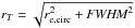
To measure the effective radius of our objects we used the 2D surface brightness fitting tool GALFIT (Peng et al. 2002, 2010). For each galaxy we chose to fit a single Sérsic profile with no constraint in the parameters. To remove the effect of the ellipticity of each source, the final size value as measured from GALFIT is computed as the circularized radius by 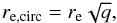 (3)where q is the axis ratio (b/a) of the elliptical isophotes that best fit the galaxy. In this sense, a comparison with rT defined in Sect. 4 is also more immediate, as both are circularized forms of size measurements. The initial parameters were retrieved from running SExtractor (Bertin & Arnouts 1996).
3.2. PSF and masks
To provide accurate size measurements it is crucial to have a good image representing the point spread function (PSF) of the data. For that purpose a list of individual, bright, non-saturated field stars were pre-selected based on their position in the stellar locus of the μmax − mag diagram. This procedure was applied to all the CANDELS, UltraVISTA and CFHTLS mosaic images. Then, we selected the stars to be used for the stack by visual inspection. Thus, we built an image with high S/N of the PSF for each image by stacking ~40 stars in each CANDELS field. For COSMOS we used the models built with TinyTim 2 described in Rhodes et al. (2007).
For space-based imaging, we fed GALFIT with 6″ × 6″ image cutouts around the galaxy. As for the masking procedure, we used the segmentation map produced by SExtractor and flagged all companion objects for which all pixels associated with it are at a distance greater than 1′′ of the VUDS target. The flagged pixels were not taken into account for the χ2 fitting by GALFIT. Based on deep galaxy counts (Capak et al. 2007) we estimated the number of companions at a distance smaller than 1′′ and brighter than iAB = 25.5 is 6%. This ensured that we obtained size measurements for sources that fall within the slits, meaning that it is unlikely that GALFIT will lock on a companion object.
3.3. Image simulations
Simulations of 15 000 galaxies using GALFIT Sérsic profiles convolved with the observed PSF were performed to test the reliability of the obtained values for the effective radius of the galaxies in the sample. To do so, we used the computed SExtractor source catalog to select 200 × 200 pixel sky regions on which the simulated galaxies were dropped. The sky regions were randomly selected so that we did not introduce artificial bias by using hand-picked regions. However, since the selection of pure sky regions in a random way is very time consuming, a method was devised to select the required size regions in a faster way while still ensuring that we did not overlap simulated and real sources and avoided bright sources within the region. This method selects random regions where without pixel detections within a 50 pixel radius from the center of the sky region, where the neighboring sources allowed in the stamp image are not brighter than 20 mag, where the number of SExtractor-detected sources within the stamp is limited to ten, and where all pixels have a non-zero value. Then the simulated galaxies have Sérsic profiles that are randomly generated from a set of values drawn from uniform distributions in the intervals defined in Table 1. The profiles were subsequently convolved with the PSF and dropped on extracted regions. Finally all the simulated objects were fed into the same pipeline as the real images to obtain their output parameters from GALFIT. The results of these simulations (see Fig. A.2) show that we can retrieve the input effective radius value within 10–20% for 68% of the simulated galaxies that have a total magnitude ≲25. There is also a slight trend with the input effective radii in the sense that galaxies with higher input re tend to have slightly higher dispersion (up to ~20–30%) of the difference that is obtained. We note, however, that 93% of the galaxies in our sample have measured radii smaller than 20 pixels for which we obtain a radius within ~15% of the input value. We tested this simulation by using different background images from which to extract the sky regions (COSMOS F814W tiles and CANDELS F814W, F125W, and F160W mosaics) and found no significant differences in the simulation results. Similar conclusions were found, for example, by Mosleh et al. (2011) and Morishita et al. (2014).
Interval of simulated values of artificial galaxies.
An additional test was carried out to test the reliability of GALFIT results against the choice of first-guess parameters. In this case, we ran GALFIT fifty times for each galaxy, each of which with a set of Gaussian randomly deviated values centered on the SExtractor input guesses and with widths that include a deviation of at least 50% from the input value within 1σ. We then compared the median value of the fifty runs with the results from the single run with SExtractor first guesses and found that no more than ~9% of the galaxies for which GALFIT converged have median values offset by more than 3σ and that most of the galaxies (~90%) are within 1σ. The outliers tend to occur for cases where GALFIT does not converge for one or more of the fifty tries. Nonetheless, the majority of the galaxies for which we have GALFIT results (around ~74%) allow the convergence more than 40 (out of 50) times.
3.4. Dependency on color
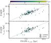 |
Fig. 4 Comparison of size measurements derived with GALFIT for a subset of 153 (118) VUDS galaxies at 2 <z< 4.5 with available F814W and F160W (F125W) images from CANDELS. Results are split into two bands: F160W in the top panel and F125W in the bottom panel. Circles and squares refer to COSMOS and ECDFS respectively. The dashed black line shows where the two radii are equal. The symbols are color coded according to their spectroscopic redshift and the mapping is shown in the colorbar at the top of the plots. Fewer galaxies are available in the J-band comparison because there are no such data available in ECDFS. |
To study size evolution across a wide redshift range, common rest-frame measurements are required whenever possible. When this is not possible, some approximations must be made. The simplest consists of using the observed band closest to the rest-frame that it is to be considered (e.g. Morishita et al. 2014; Shibuya et al. 2015). A more evolved approach has been presented by van der Wel et al. (2014), who observed and fit a wavelength dependence of the measured radii. A correction is then applied to each galaxy to obtain the value of the radius at exactly the chosen wavelength. However, such approaches require a multiwavelength coverage of the targets which is not available for the majority of our sample.
For the galaxies that lie in the CANDELS area (roughly 10% of our sample), we computed the effective radii in three different bands: F814W, F125W and F160W. Based on an inter-wavelength comparison we found that the derived sizes are similar in all three bands (see Fig. 4). We report a small offset in the median values of rI − rH ≈ −0.04 kpc and rI − rJ ≈ −0.01 kpc. The dispersion on the size measurements across different bands is 0.21 dex and 0.20 dex for comparisons of F814W–F160W and F814W–F125W, respectively. For a more detailed inspection, we used the wealth of multiwavelength observations of the COSMOS field (space- and ground-based imaging) with a variety of instruments from three different surveys (CFHTLS in the optical and WIRDS and UltraVISTA in the near-infrared) to obtain size measurements up to the Ks band, which at the highest redshifts considered here still probes the regions above the Balmer/Dn4000 break. Then, for each galaxy in our sample, we plot its size value as a function of the observed wavelength computed using the knowledge of the spectroscopic redshift and the filter wavelength, λF,  (4)Size measurement results at different wavelengths obtained from our galaxies are presented in Fig. 5. The overall trend is that at the redshifts considered here, measurements of circularized effective radii are independent of wavelength to first order. This result tells us that circularized effective radii computed from F814W observations are not much affected by the rest-frame wavelength at which the galaxies are observed. To quantify the wavelength dependence, we fit the relation
 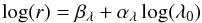 (5)to all the data points considering space-based imaging and ground-based imaging separately. We find that for ground based data (covering from I to Ks bands) the slopes measured are all consistent with no wavelength dependence (αλ = 0 is within 1σ at all redshift intervals). For space-based data (covering from I to H bands) we find slightly positive slopes indicating slightly larger sizes in the redder bands, but only marginally significant 1.9σ away from a flat slope αλ = 0. Using our fit values in Eq. (5) we estimate that the ratio ranges within r1700 Å/r2500 Å = 0.89–1.01.
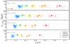 |
Fig. 5 Measured sizes as a function of wavelength for galaxies with log 10(M⋆) > 9.5 at 2 <z< 4.5 in the COSMOS field. Different symbols correspond to different surveys (symbol coding in the bottom panel) and different colors to different observed bands (color coding in the top panel). Each point represents the size of a given galaxy at the rest-frame wavelength of the pivot of the filter. |
In a complementary test, we fit the size-wavelength relation for all individual galaxies with measurements in three or more bands. The median slope is αλ = 0.03 ± 0.27 and αλ = −0.12 ± 0.34 for space- and ground-based observations, respectively. This translates into a ratio r1700 Å/r2500 Å = 0.99(1.05) for space- (ground-) based data. This supports the fact that the wavelength dependence of galaxies in our sample is very shallow and consistent with no dependence at all for the ensemble of the galaxies in our sample. We note, howeve,r that there is a large dispersion among our galaxies, which means that the wavelength dependence requires a different treatment when considering them on a case-by-case basis.
We showed in Fig. 5 that we can measure sizes from ground-based data for the galaxies in our sample. This would allow for the use of the entire VUDS sample, including galaxies in the VVDS-2h field. However, since the convergence success of GALFIT is much lower (~30%) and because the method described in Sect. 4 is PSF dominated, we are prevented from obtaining galaxy sizes (sizes are systematically overestimated when compared to those obtained with HST images) and opted to conduct our analysis on space-based data alone.
3.5. Results: re measurements
 |
Fig. 6 Size distribution for different redshift bins. The vertical dashed line indicates the median value for each bin. The black line is the fit of the distribution using a normal function in log space. |
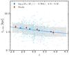 |
Fig. 7 Size evolution with redshift. Each galaxy with a good size measurement is plotted with a small blue point (squares for redshift confidence 2 and 9, circles for 3 and 4). The median values (in redshift and size for each bin) and respective error ( |

We fit all galaxies in the stellar-mass-selected sample using the automated GALFIT procedure described in the previous sections to obtain effective size measurements re. After fitting all galaxies, a subset of 19.5% of those GALFIT failed to converge. These galaxies were analyzed on an object-per-object basis and a manual refitting was attempted by tuning the initial set of parameters. After this manual try, of the 1242 galaxies in our stellar-mass-selected sample, 263 (15.7%) objects have no structural parameters because GALFIT failed to converge. These objects typically have very low surface brightness or are highly concentrated galaxies.
The size distributions presented in Fig. 6 show similar shapes at all redshifts, showing a slow monotonic decrease in their median sizes as redshift increases. Each distribution is fit with a normal function (in log space) and the derived sigma values from the fit are similar at all redshifts (0.23, 0.26, 0.29 and 0.24 with growing redshift).
The overall evolution of sizes across the redshifts considered here is shown in Fig. 7. We find that the effective radius of galaxies continuously decreases over the redshift range of our sample. Galaxies with 2 <z< 2.5 have ⟨re,circ⟩ = 1.67 ± 0.09 kpc, while in 4 <z< 4.5 the median effective radius is a factor of 1.6 smaller, ⟨re,circ⟩ = 1.05 ± 0.05 kpc. In every redshift bin a large dispersion in the effective radii is measured among the galaxy population and for all redshift bins ~9% of the population has measured radii that are large (re,circ> 3 kpc) and some extremely so (7–10 kpc) in all redshift bins save the last. These features of the distribution are discussed together with other measurements in Sects. 6 and 9.
3.6. Effect of cosmological dimming on re
A key point to take into account in this analysis is that GALFIT-based measurements do not take the surface brightness (SB) dimming effect into account. This effect is a strong function of redshift. Parametric modeling works well even under low S/N conditions3, recovering the correct parameter values, although with larger uncertainties. This should, in principle, deal with the increased SB dimming of galaxies at higher redshift. The dimming effect, if significant, would act in the sense of obtaining smaller sizes at higher redshifts that would in turn affect the derived evolution in that it would shoe a steeper slope. Thus, a correction for the cosmological dimming could lead to a weaker size evolution.
We tested this scenario by masking the pixels that are below the surface brightness threshold we used (see Sect. 4.3) and then ran GALFIT to obtain the size measurements from this pixel set reduced to the brightest regions of galaxies. GALFIT found similar sizes for cases with and without masking these low surface brightness pixels, and that the trend in evolution was not affected.
4. Galaxy area and equivalent radius rT
While the local Universe is dominated by galaxies with symmetric shape in the form of disks and bulges, the distribution of galaxy shapes becomes more complex with increasing redshift. By redshift z ~ 1–2, irregular galaxies make up to 52% of the population of galaxies (Delgado-Serrano et al. 2010; Huertas-Company et al. 2015). By redshift z ~ 3, galaxies with irregular shapes dominate as they represent ~65(40)% of the population of massive, log 10(M⋆) > 10(11), galaxies (Mortlock et al. 2013; Buitrago et al. 2013). These irregular shapes often have the form of clumpy galaxies representing ~60% of the star-forming galaxies at 2 <z< 3 (e.g. Elmegreen et al. 2007, 2009; Wuyts et al. 2012; Guo et al. 2015; Huertas-Company et al. 2015). This fraction might be higher at higher redshifts (Conselice & Arnold 2009). Irregular shapes can take very diverse forms, including objects with one single asymmetric component, with multiple components, with a tadpole shape, extended with low surface brightness, and can be confused in the presence of close projected or physical companions. Some examples of galaxies in our sample are shown in Fig. 9. The fit with GALFIT gives an effective radius that highly depends on the relative brightness of each clump of the galaxy, but the residuals after fitting show how difficult it is to fit such an object with a symmetric profile.
These considerations prompted us to use other ways than parametric fitting to derive sizes of galaxies. A non-parametric definition removes the need for assuming a surface brightness profile. Measuring the half-light radius based on SExtractor and/or curve-of-growth methods is also widely used (e.g. Ferguson et al. 2004; Bouwens et al. 2004; Hathi et al. 2008; Oesch et al. 2010; Curtis-Lake et al. 2016). However, these non-parametric methods require a center and an aperture definition to be computed. Such quantities can, again, be misleading in cases of highly disturbed morphology.
With this in mind, we developed a simple size estimator based on the total area covered by a galaxy above a given surface brightness threshold. In the following sections we define a non-parametric size measurement independent of any assumption related to a symmetric light distribution. This method is more affected by PSF broadening and noise at low surface brightness than parametric fitting. Nonetheless it has the advantage of being independent of the shape of the galaxy, and nicely complements the standard re measurements. The other advantage of this method is that it does not depend on initial guesses and does not require a fit to converge.
4.1. Method
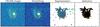 |
Fig. 8 Illustration of the size measurement process for VUDS 510799304 at z = 2.4281. From left to right: (1) the original F814W image from COSMOS (Koekemoer et al. 2007). (2) The same image after smoothing by a Gaussian kernel of 1 pixel width and extending over four times the width. This kernel ensures an improvement in signal to noise for low surface brightness levels while preventing a significant boost of noisy pixels, which would incidentally increase the measured radius if the kernel were too large. (3) The segmentation map obtained after running the detection algorithm including all pixels greater than kσ. (4) The selection of the target galaxy. All panels have 1.77′′by 1.77′′and the orange circle has a radius of 0.5′′. The total size is computed from the number of pixels in the last panel. |
We defined the area of a galaxy by counting the number of pixels above a given surface brightness threshold that belong to it. This approach has the advantage of being completely independent of any asymmetries that the galaxy may have and does not require any centroid or aperture definition. As most of the objects in our sample show irregular morphologies, we defined physical sizes using the total area Tx as (adapted from Law et al. 2007)  (6)where Nx is the number of pixels of size L (in arcsec/pixel) that sum to x% of the galaxy measured flux and DA is the angular diameter distance derived using cosmological parameters. From this we can define the area equivalent radius,
  ,
,  (7)In the following we use T100 and
  , the area and the equivalent circularized radius that enclose 100% of the measured flux above a given surface brightness threshold. The quantity
  , the radius equivalent to the area that sums to 50% of the total galaxy light, is similar to the effective radius derived from the GALFIT profile fitting, but taking into account irregular and asymmetric morphology. We also use the values of
  and
and  enclosing 80% and 20% of the flux, respectively.
In practice, the method works as follows.
-
1.
We smooth an image stamp of 6″ × 6″ centered on the VUDS galaxy with a Gaussian kernel with 1 pixel sigma width, truncated at 4 pixels.
-
2.
We compute the segmentation map of the smoothed image based on a given surface brightness threshold.
-
3.
From the segmentation map we select the area of connected pixels that contains the brightest pixel within a 0.5 arcsec radius from the target coordinates.
-
4.
Using the selected pixels, we compute the total flux of the galaxy by summing the flux in each pixel.
-
5.
Finally, we iterate (using 1000 steps) fi from the maximum to the minimum flux detected within the segmentation map. At each step we compute the summed flux from the pixels for which fpixel>fi. When the summed flux corresponds to x% of the galaxy total flux, we store the number of pixels that have fluxes greater than fi at that step and then compute Tx using Eq. (6).
The selection method chosen for the purpose of this project has the main goal of minimizing the effect of neighbor contamination and of not imposing any size constraints on the derived measurements. We tested two other different methods: selecting the largest area or the brightest area (by summing the fluxes of all its pixels) for which a subset of its pixels is inside the 0.5′′radius. Both methods yield similar results.
We have tested the contamination by neighbors dropping simulated galaxies in random regions of the images with and without a constraint on the presence of sources within 2.0 arcsec of the simulated galaxy. When no constraints were imposed, the sizes were sometimes artificially increased by the area occupied by a neighboring source. Still, the rate of contamination does not dominate the measurements. The percentage of simulated galaxies with recovered sizes twice as large as the input is of 8% for the random clean regions and 17% for the purely random regions. We expect that the contamination rate of our galaxies will be closer to the first reported value because as a result of the data processing for a spectroscopic survey, galaxies with large bright companions are excluded from the sample owing to problematic redshift estimation.
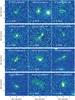 |
Fig. 9 F814W imaging in COSMOS (Koekemoer et al. 2007) and CANDELS (when available, Koekemoer et al. 2011) of the measured sizes for three galaxies in each of four increasing redshift bins from z ~ 2.4 to z ~ 4.1 (top to bottom) in our sample. The green contours show a smoothed version of the segmentation map of the galaxy at the defined threshold, which translates into T100 from Eq. (6) measured at kp = 1.0. The black ellipses are constructed from the values of re,b/a and θPA derived from GALFIT for those galaxies. The parametric and symmetric 2D profile fitting with GALFIT fails to properly account for the complex irregular morphology when deriving the size of galaxies at these redshifts, while the non-parametric method presented in this paper is able to derive more realistic sizes. |
4.2. Cosmological dimming and luminosity evolution
Tolman (1930) demonstrated that in an expanding Universe the relation between the flux and angular size of a nebula should follow the relation (adapted from his Eq. (30))  (8)At the time (see Lubin & Sandage 2001) this was the only observational test that was proposed to confirm the reality of the expansion of the Universe, which is now well established. This dimming effect, independent of the cosmological model, has to be taken into account to measure galaxy sizes (by means of counting pixels) at the same surface brightness level at different redshifts.
However, when the image recorded with the detector is analyzed, the number of detected photons arriving from the observed source is considered, and not at an integrated flux. We consider a square region of the emitting source corresponding to the pixel size at the location of the object. The monochromatic energy emitted is given by  (9)which, for a source emitting at constant brightness inside that pixel simplifies as
  (10)where T is the physical size of that pixel. Considering a pixel size p, the physical size, in kiloparsec, is proportional to:
  (11)At a distance DL the observed light is
  (12)The number of observed photons is
  (13)Combining the equations above, we obtain
  (14)With DL = DA(1 + z)2, the number of observed photons per unit area is
  (15)The factor I/ (hνe) represents the number of emitted photons per unit area. The same redshift dependence was found by Giavalisco et al. (1996), and it was used in Law et al. (2007).
In addition to the dimming effect, the average evolution in luminosity of a population of galaxies has an effect on the typical threshold defined at any given redshift. This means that a galaxy with a fixed size but with an increased luminosity because of luminosity evolution will appear larger above a fixed luminosity threshold. The average luminosity evolution from z ~ 4.5 to z ~ 2 as reported in the literature is 0.4 mag in the UV rest-frame Reddy & Steidel (2009), Bouwens et al. (2015).We took this effect into account by parameterizing the evolution of the characteristic luminosity L∗ within the redshift range considered. Taking the L∗ values in Reddy & Steidel (2009) at z< 3 and those from Bouwens et al. (2015) at z> 4, we defined a broken luminosity evolution that is steeper below z< 3 and flattens at z> 4:  (16)
(16)
4.3. Detection threshold
The dimming effect described in the previous subsection relates to an important tuning parameter for this non-parametric size measurement which is the detection threshold above which a pixel is classified as a detection and may be assigned to the galaxy. This detection threshold is defined as a multiple k of the standard deviation of the sky emission, σ, computed globally. To ensure that we compare galaxies imaged at different depths, the value of σ is taken as the median standard deviation of the image noise computed from 100 different regions in the shallowest survey. In our case, σ = 1.1 × 10⁻¹⁴ erg s-1 cm-2 arcsec-2 was computed from the COSMOS images.
The choice of k plays an important role on the size estimates that are obtained. The simplest assumption is to define a constant value k0 across all redshifts. Another approach consists of taking the effect of cosmological dimming and typical luminosity evolution (described above) into account and choosing k as a function of the galaxy redshift following  (17)where kp is the value of k at the pivot redshift zp and L(z) is defined in Eq. (16). To use this method, the availability of spectroscopic redshifts is even more important as errors in redshift would affect the threshold used and consequently influence the final size measurements of the galaxies.
The drastic evolution of the detection threshold (see Fig. 10) led us to restrict the redshift interval of our study to 2 <z< 4.5. In this range we probed the total extent of galaxies down to a lower surface brightness level at lower redshift while we avoided overestimating galaxy sizes at the high-redshift end that are due to random sky background noise detection. To obtain a size measurement corresponding as closely as possible to the total physical area covered by a galaxy, the choice of the threshold was based on the average number of connected sky pixels as a function of the threshold. This is at the level of 1.0σ, where we start to detect connected pixels (4–6 pixels) only due to random sky noise fluctuations. Based on this, and on the average galaxy color, which we discuss in Sect. 4.5, we defined k such that at z = 2 it has a value of 1.0 to probe galaxies down to their fainter regions. This corresponds to a detection limit of ≈0.25σ per pixel at z = 4.5. We discuss the contamination from random fluctuations and the correction made to the size measurements measured down to these thresholds in Sect. 4.6.
The galaxy sizes that we measure are tied to the choice of kp and/or the depth of the image that determines the value of σ. By setting the value of k × σ at higher or lower values, the absolute value for the galaxy size will decrease or increase, respectively. We therefore report total size measurements indexed to a specific choice of kp, that is, to a specific limiting isophote defined at z = zp. For the sake of simplicity we refer hereafter to our non-parametric size as the total size.
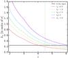 |
Fig. 10 Value of k as a function of redshift for different choices of kp. The vertical dotted line shoes the upper redshift limit we assume in this paper. The black solid line shows the depth limit above which the noise correction is larger than 100 pixels. |
4.4. Correcting for PSF broadening
Because we measure sizes directly on images, the broadening of the profile by the instrumental PSF affects our results. To correct for this effect, we simulated with GALFIT a PSF image rescaled to match the magnitude of the galaxy. We then ran the simulated PSF through the same detection algorithm and obtained the size of the PSF at the object magnitude and same surface brightness level. We then computed the galaxy size by correcting for the PSF broadening using the following formula 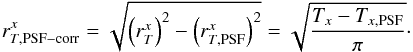 (18)
(18)
4.5. Dependency on color
The method of measuring galaxy sizes presented above is dependent on individual pixel detection, and it is therefore more sensitive to the galaxy spectral energy distribution than other methods relying on a given surface brightness profile. Even in the absence of color gradients, the simple fact that one object might have a wavelength-dependent brightness causes the number of selected pixels to vary owing to the relative brightness change in the galaxy within a given filter with respect to the detection threshold.
To correct for this we applied a simple color correction to the detection threshold that takes the different brightness at different rest-frame wavelengths into account: 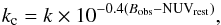 (19)where k is that of Eq. (17) and (Bobs − NUVrest) is the color term. The color is defined to be the observed band, B, minus the rest-frame NUV band derived from SED fitting with LePhare. The choice of the NUV band was made such that for the majority of our galaxies, the color term is minimal since it overlaps with the observed band.
We compared the PSF-corrected values of  derived in the F814W, F125W, and F160W bands in Fig. 11 (see also Fig. 12). We report a small offset in the median values of rI − rH ≈ −0.08 kpc and rI − rJ ≈ 0.51 kpc. The dispersion on the size measurements across different bands is 0.27 dex and 0.22 dex for the F814W–F160W and F814W–F125W comparisons, respectively. We stress that part of the scatter observed in this figure is due to the color correction described above which is sensitive to the objects’ magnitude in each of the bands. This in turns affects the final isophote threshold and therefore the final measurements. Nonetheless, we highlight that we observe no large systematic offsets in the comparison between the I and H bands.
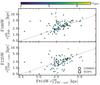 |
Fig. 11 Comparison of |

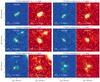 |
Fig. 12 F814W (in blue) and F160W (in red) imaging in CANDELS (Koekemoer et al. 2011) of six example galaxies in VUDS. The green contours show the isophote used to derive |
4.6. Correcting for sky pixel detection
In the presence of uncorrelated Gaussian noise, the probability of a sky pixel to lie above the detection threshold defined above is not negligible. To estimate the level of contamination produced by random sky noise, we computed the N100 area (Eq. (6), size of the segmentation map) on a search radius of 0.5 arcsec (the same as when computing T100 for the real galaxies) randomly selected on 500 300″ × 300″ regions.
For each search radius, we computed the area defined for surface brightness thresholds ranging from 0.05σ to 2.05σ using steps of 0.025. This provides the median area of sky connected pixels for a given threshold value. We used this to correct the value of  following
  (20)where Tsky(k) is the median number of connected sky pixels at a threshold k. In Fig. A.1 we show the effect of this correction on a set of simulated galaxies. We stress that this correction is only applied to the value of . We note, however, that the effect of the noise is greater when the fraction of the flux used to derive sizes is increased. Sky noise effects are negligible for sizes computed using 10% of the total flux.
4.7. Results
Of the 1242 galaxies in our stellar-mass-selected sample, 67 objects have no measured value of rT. These failures are due to the lack of pixel fluxes above the selection threshold defined in Eq. (19) for 17 objects and to the lack of color information for five objects. The other 45 objects are on the edge of the image mosaic, and thus no sufficient information is available to derive a size.
The distribution of total sizes is presented in Fig. 13 for the four redshift bins previously defined. The shape of the distribution remains roughly the same with redshift. The Gaussian fit on each subsample yields sigma values of (0.154, 0.141, 0.168, and 0.154) with increasing redshift.
We compare the total size measurements to the circularized effective radius obtained in Sect. 3.5 in Fig. 14. Galaxies with larger re,circ are also larger in total size. However, this trend deviates from the linear relation and there is a large scatter in the relation. The scatter is somewhat expected because the galaxies have highly irregular morphologies. While GALFIT gives a heavier weight to the brightest pixels (which can be locked into a single bright clump in a large galaxy), rT measures the whole galaxy extent. GALFIT can pick up fainter buried flux of a galaxy by extrapolating the profile measured on the bright pixels, which is not picked up when computing the total size using our method. This explains why some galaxies have re,circ larger than rT. It is interesting to note that the  is nicely correlated with re,circ, as shown in Figure 14, with a dispersion of 0.23 dex which is a consequence of the frequent asymmetric shapes in our sample.
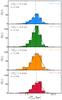 |
Fig. 13 Total size distribution for different redshift bins. The vertical dotted line indicates the median value for each bin. The black line is the fit of the distribution using a normal function in log space. |
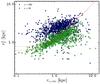 |
Fig. 14 Comparison of the two size estimates. With dark blue points we show the comparison to |


The evolution of total sizes across the redshifts considered here is shown in Fig. 15. Total sizes remain roughly constant over the redshift range 2 <z< 4.5, with  kpc. The dispersion around the mean of σ ≃ 0.9 kpc (0.21 dex), and we find galaxies that are as large as ~5.5 kpc and as small as ~0.5 kpc at all redshifts in this range. Size measurements using this definition are consistently larger than sizes provided by the effective radius re. This is discussed in Sects. 6 and 8.
We show the dependence of the absolute value of the measured sizes as a function of the chosen value of kp in Fig. 16. As expected, using different limiting isophotes over a range of 2.5 in luminosity changes the size values. It is therefore essential to quote the absolute luminosity of the isophote used to compute galaxy sizes. We note that at all times, the observed trends as a function of redshift are consistently different from those observed with GALFIT, with approximately constant sizes as a function of redshift while the effective radius is observed to decrease strongly.
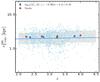 |
Fig. 15 Total size evolution with redshift. Each galaxy is plotted with a small blue point (squares for redshift confidence 2 and 9, circles for 3 and 4). The median values and respective error ( |
 |
Fig. 16 Total size measurements defined at different values of kp that correspond to different luminosity thresholds at z = 2. From top to bottom, the colored circles correspond to kp = 0.8,1.0,1.2,1.5, and 2.0. The color coding is the same as in Fig. 10. |
5. Average galaxy profiles and light concentration
Since the total sizes of galaxies, measured at the same surface brightness level, seem to evolve not much with redshift, we investigated whether the same pattern applies to the light profiles. We did this by considering the stacked profiles and the individual measurements of light concentration in galaxies.
5.1. Image stacks
To investigate the evolution of the light profiles we stacked images of the large number of sources in our sample to follow the profile at larger radii than from individual images. The stacking procedure started by us collecting a 10″ × 10″ stamp image for each galaxy in the sample. Then, we ran SExtractor to find the light-weighted center of each source. We shifted the image by the difference between the light-weighted center and the physical image center, using a cubic spline interpolation to rescale the image onto a common grid. After processing the entire sample for a given redshift bin, we took the median pixel value as the flux of the stacked image at each position. We also produced a straightforward sum to the images normalized by the total galaxy flux. The results of both methods give the same qualitative answers.
Stacking within a redshift bin, smears the rest-frame light over the interval. In addition, when comparing different redshift bins we effectively consider different rest-frame light. This ranges from ~2500 Å in the lowest redshift bin down to ~1600 Å in the highest redshift bin. As shown in Sect. 3.4, the sizes derived are roughly the same across this wavelength range. This difference in rest-frame wavelengths has no effect on the comparison of the profiles discussed in the next section.
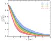 |
Fig. 17 Normalized surface luminosity profiles of the median stacked F814W band images of galaxies in our sample at four different redshift bins (normalized at r = 0.3 kpc). The width of each profile encodes the surface luminosity error. This profile comparison shows the increased light concentration at higher redshifts. |
5.2. Luminosity profiles
The redshift dependency of the light profile derived from the stacked images is presented in Fig. 17. We converted the median stacked profiles into surface luminosity profiles and show these profiles normalized at r = 0.3 kpc. The light profiles change smoothly across redshift starting from a highly peaked, concentrated profile at the higher redshifts z ~ 4 and becoming less concentrated at the lower redshifts z ~ 2.25.
5.3. Light concentration of individual galaxies
To further investigate the change in light profiles with redshift, we used a different but quite commonly used way to quantify the light concentration. The concentration parameter was originally defined by Bershady et al. (2000) as the ratio of the 80% and 20% light radius derived from elliptical apertures centered on the galaxy. This measurement assumes symmetrical isophotes to derive the galaxy concentration, which makes it difficult to apply to irregular and asymmetric galaxies at high redshifts as is the case of our sample. To overcome this limitation we derived the concentration parameter CT, using  and
and  as defined in Sect. 4, generalizing the computation of C to the case of irregular and asymmetric galaxies
 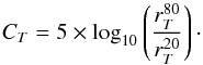 (21)We plot the evolution of CT in Fig. 18. In this figure we show the fit of the equation
 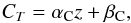 (22)and find a value of αC = 0.23 ± 0.02 and βC = 1.64 ± 0.06. Thus, CT strongly evolves with redshift, light being more concentrated at higher redshifts. The concentration CT increases by ~25% from z ~ 2 to z ~ 4.5.
Using the standard definition of concentration with symmetric apertures (see Appendix B for details on the computation) leads to an different trend (αC = 0.01 ± 0.04 and β = 2.82 ± 0.13) with light concentration being rather constant within our redshift interval. This difference is easily explained as caused by the effect of defining a galaxy center for irregular morphology. For instance, on a galaxy composed of several same-brightness level clumps, the center of light would be defined somewhere in between the clumps, which would lead to a lower concentration because the radius containing 20% of the total light would be larger to include the clumps.
The concentration values derived for the median stack images report the same trend as those derived from the full sample (Fig. 18). While the concentration value for the stacked images is sensitive to the threshold definition (average color and kp from Eq. (17)) the evolution trend remains unaffected and the slope is rather stable.
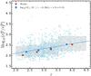 |
Fig. 18 Evolution of light concentration in galaxies computed from the ratio of the non-parametric radii enclosing 80% and 20% of the total flux, as defined in Sect. 4. The solid line is a linear fit to all the small blue points. Each galaxy is plotted with a small blue point (squares for redshift confidence 2 and 9, circles for 3 and 4). The median values and respective error ( |
6. Size evolution with redshift
In Sects. 3.5 and 4.7 we mentioned that we were unable to obtain galaxy sizes for the entirety of our sample for each of the measurements presented and for different reasons in each case. We tested a scenario where we removed from the sample all galaxies without both size measurements, which comprise 238 (19%) of the stellar mass selected sample. The results did not change when these objects were removed, and therefore we kept them in the final sample for the individual analysis of rT and re to reduce the statistical errors in our measurements.
Median size values (for F814W, in kiloparsecs) per redshift bin considered here.
Best-fit slope and normalization factor for equation log (r) = αrlog (1 + z) + βr for the different size estimates used throughout the paper.
To quantify the redshift evolution of sizes, we fit the data points with a commonly used parameterization (e.g. Shibuya et al. 2015; Straatman et al. 2015; van der Wel et al. 2014; Morishita et al. 2014):  (23)We fit this relation to all galaxies with a size measurement weighted equally due to the lack of individual errors on . The sample variance of the parameters βr and αr was obtained from bootstrapping the data 5000 times using 80% of the full sample each time. The resulting fits through the data are plotted in Figs. 7 and 15. We also computed the same evolutionary trend for different values of x of Eq. (6) ranging form 10% up to 100% with a 10% step value. All the fit results are given in Tables 2 and 3 and summarized in Fig. 19.
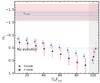 |
Fig. 19 Slope of the evolution of PSF corrected galaxy sizes as a function of the flux level considered. The light colored symbols correspond to the slope computed from sky-corrected |
Figure 19 encodes the information on the slope of the size evolution as a function of the flux level and compares it to the effective radius evolution derived from GALFIT. There are three main points to be taken from this figure. First, there is a clear trend of the slope as a function of the flux cut level: the brightest regions (10% brightest pixels) evolve faster than the total size with a smooth trend toward slower evolution from the brightest regions to the total area of the objects. This differential trend is again an indication of the evolution of light concentration as a function of redshift where the brightest regions of the galaxy tend to become larger with time while the total size remains constant, effectively suggesting that light becomes less concentrated with time. Second, the evolution in sizes is far different from that reported from the effective radii re,circ. For the size measurements including the brightest pixels that amount to 50% of the total flux (comparable to re), the derived evolution slopes are separated by more than 3σ (Fig. 19) indicating that the choice of method to compute sizes can have a very significant effect on the observed evolution. We note that the points in Fig. 19 indicate the lower limits on the slope. At the highest redshifts a galaxy size will be more often overestimated because lower flux thresholds increase noise contamination. We attempted to correct for that using the prescription described in Sect. 4.6, but it applies only to . However, this effect cannot explain the observed difference between re and rT as the size evolution slope after the said correction still differs by more that 3σ from that derived from re,circ and it is where the effect of the noise affects the slope the most.
6.1. Effective radius re evolution
The galaxy size evolution derived from the circularized effective half-light radius shows strong size evolution across the redshift range probed. Assuming that galaxy sizes evolve according to the parametrization of Eq. (23), we derive a slope of αr = −1.29 ± 0.18.
Values reported in the literature range from αr = −0.56 ± 0.09 for a sample of star-forming spectroscopically confirmed galaxies at 0.5 <z< 3.0 with log 10(M⋆/M⊙) > 10 (Morishita et al. 2014) up to αr = −1.32 ± 0.52 for a sample of LBGs with (0.12–0.3)L⋆ at z ~ 4–6 (Oesch et al. 2010). The differences between these results (see also Ferguson et al. 2004; Bouwens et al. 2004; Trujillo et al. 2006; Franx et al. 2008; Williams et al. 2010; Mosleh et al. 2011, 2012; Ono et al. 2013; van der Wel et al. 2014; Morishita et al. 2014; Curtis-Lake et al. 2016; Shibuya et al. 2015; Straatman et al. 2015) can be traced to different likely sources: (1) the samples are selected in different ways; (2) there are two different methods for measuring sizes, both relying on a certain degree of symmetry; and perhaps most importantly; (3) samples with different stellar masses yield different sizes (Franx et al. 2008; van der Wel et al. 2014).
6.2. Total size rtot evolution
The typical total size of an SFG, corrected for sky noise contamination as computed in Sect. 4, is  kpc and shows negligible evolution of galaxy sizes across the redshifts probed here (see the light color points of Fig. 19). This is markedly different from what is observed using the standard effective radii measurement. The measurements are consistent with the results of Law et al. (2007), who reported only a small increase in the the total area from z ~ 2 to z ~ 3 (T = 15.0 ± 0.7 and 17.4 ± 0.9 kpc2, respectively). This corresponds to an equivalent radius of rT = 2.19 ± 0.47 kpc at z ~ 2 and rT = 2.35 ± 0.54 kpc at z ~ 3.
7. Size relations with physical parameters
To further explore the properties of galaxies with different sizes, we compared galaxy sizes to several key physical parameters characterizing galaxies including stellar mass, SFR, age, metallicity, and dust extinction. We also investigated any possible relation between sizes and intergalactic medium (IGM) transmission toward the galaxies. These parameters were derived from the simultaneous SED fitting of the VUDS spectra and all multiwavelength photometry available for each galaxy, using the code GOSSIP+ as described by Thomas et al. (2016). This method expands the now classical SED fitting technique to the use of UV rest-frame spectra in addition to photometry, further improving the accuracy of key physical parameter measurements (see Thomas et al. 2016, for details).
The distributions of re,circ and  sizes versus M⋆, SFR, age, AV, and IGM transmission are presented in Fig. 20. Several interesting trends can be observed. To quantify the degree of correlation of each parameter with size, we used the Pearson (1896) correlation coefficient. In our sample, the null hypothesis (i.e., no correlation) is excluded at the 3σ level if | r(Pearson) | > 0.12
Our data show a correlation between galaxy size and M⋆ with larger galaxies having on average higher stellar masses. This supports the correlation reported from other samples (e.g Franx et al. 2008; Ichikawa et al. 2012; van der Wel et al. 2014; Morishita et al. 2014) at redshifts z> 2 and extends it up to z ≃ 4.5. This correlation is of similar strength for as is for re. We obtain r(Pearson) = 0.08 for against r(Pearson) = 0.13 for re. Interestingly, the most massive galaxies in our sample show a break at stellar masses higher than log 10(M⋆/M⊙) > 10.5 in this correlation. While, when re,circ is considered, sizes become smaller, sizes computed from increase at higher stellar masses. This partly supports our analysis that low surface brightness regions in massive galaxies with complex morphology are not taken into account by parametric fitting as is done in GALFIT, resulting in an artificially smaller effective radius (by a factor of ~2).
The SFR is strongly related to galaxy sizes. For sizes measured with we find that larger galaxies have higher star-formation rates, with a positive correlation (r(Pearson) = 0.29). The correlation is not significant with r(Pearson) = 0.03 for re,circ. Considering the M⋆-SFR main-sequence of star-forming galaxies in VUDS (Tasca et al. 2015), this correlation may partly reflect the underlying stellar mass-size relation described above.
Galaxies appear to be older when they are smaller based on the relation between age (as defined by the start of star formation, see Thomas et al. 2016) and (r(Pearson) = −0.21). Based on the hierarchical assembly scenario we would expect that larger galaxies have older stellar populations. On the other hand, the less significant relation between re,circ and age (r(Pearson) = −0.10) may also mean that the derived age is dominated by the age of the last major burst of star formation, which overshadows the underlying older stellar populations that may exist in the central brightest clumps from previous starburst episodes.
Galaxies with lower extinction values have smaller median sizes than galaxies with higher dust extinction. This trend is more significant for (r(Pearson) = 0.13) than it is for re,circ (r(Pearson) = 0.03). This indicates that extended regions of galaxies have a higher dust content than smaller ones.
The projected stellar density computed as the ratio of the stellar mass to the projected area of a galaxy is shown in Fig. 21. We observe a strong correlation for both (r(Pearson) = 0.59) and re,circ (r(Pearson) = 0.36). Galaxies with higher stellar masses have higher stellar mass densities.
We do not observe any significant correlation between galaxy sizes and metallicity or IGM transmission for any of our measurements.
The analysis of spectral properties such as the strength of the Lyman-α line as a function of size will be the subject of a forthcoming paper (Ribeiro et al., in prep.).
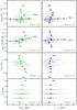 |
Fig. 20 Correlation of the measured galaxy sizes with parameters derived from GOSSIP+ SED fitting for our stellar-mass-selected sample (using the stellar masses derived with GOSSIP + and Eq. (1)). Only galaxies with good and excellent spectrophotometric fits are included. From top to bottom we show the stellar mass, SFR, age, and dust extinction. In the right panels we show the results for GALFIT derived re,circ and in the left panels we show the results for our value of |
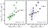 |
Fig. 21 Stellar mass surface density as a function of stellar mass. In the right panels we show the results for GALFIT derived re,circ and in the left panels we show the results for our value of |
8. Discussion
We summarize our measurements of the size evolution of star-forming galaxies with 2 <z< 4.5 in the VUDS survey, and compare them with the literature in Fig. 22.
In the context of the hierarchical assembly of dark matter halos, we can consider that the size of a disk galaxy scales with the virial radius of its host halo. In this scenario, the redshift evolution of galaxy sizes has a slope αr = −1 for halos with fixed mass and a slope of αr = −1.5 for halos with fixed circular velocity (see Ferguson et al. 2004; Stringer et al. 2014, and references therein). When we consider the effective radius, we obtain a slope αr = −1.29 ± 0.18, which lies between the values expected for these two scenarios. However, our computation of the evolution of the total size of each galaxy (measured at the same surface brightness level), leads to a slope αr = 0.13 ± 0.12 inconsistent with either of these two hypotheses. This likely occurs because we consider a majority of galaxies that do not resemble disks (i.e they are highly irregular) and, without any constraint on the profile shapes, the size measurements cannot be compared to any of those scenarios. This suggests that to correlate the size growth of galaxies with that of its host dark matter halo, more complex analytical models or more realistic numerical simulations are required to estimate galaxy and halo sizes.
The effective radius re,circ decreases with increasing redshift, indicating effective radii re,circ ~ 2 kpc at z ~ 2, and a value twice lower at z ~ 4 at re,circ ≃ 1 kpc. The effective radius measured in our galaxies is comparable to other re,circ measurements in the literature for galaxies at close or similar redshifts, particularly when compared to samples with similar stellar masses (Fig. 22). In these samples, as in our own, this leads to the conclusion that galaxies decrease in size at higher redshifts (e.g. Mosleh et al. 2011, 2012; van der Wel et al. 2014; Morishita et al. 2014; Shibuya et al. 2015). However, we argue that the use of this metric, which makes an a priori assumption of symmetry is not appropriate for constraining the redshift evolution of galaxy sizes when asymmetric and multicomponent shapes are common occurrences.
However, when we measured a size based on the total area covered by a galaxy, the evolution of size with redshift is strikingly different. This size measured at an isophote with an absolute luminosity log 10(Lz = 2) = 6.1 L⊙ pc2, after correcting for the effects of surface brightness dimming and luminosity evolution, remains approximately constant with redshift with  kpc (Fig. 22). In addition, galaxies selected using an evolving stellar mass cutoff log (M⋆) > −0.204(z − 4.5) + 9.35, have a higher concentration index CT, which indicates a more peaked light distribution at the highest redshifts, with a significant change of CT by ~20% over only ~2 Gyr of evolution.
While it is expected that the effective radius should be smaller than a radius defined from the total size of a galaxy at a much fainter isophote level, the strong observed differential evolution between the two is likely to be resulting from strong physical processes working at a cosmic time when galaxies are still early in their assembly process. The fact that the size remains large at all redshifts indicates that galaxies in their early assembly phase are quite extended with a constant characteristic size, and that the initial collapse that led to star formation seems to have been spread out in quite a large volume of ~10 kpc3.
The large dispersion observed around the mean size value may indicate quite a diversity of initial assembly conditions. We find a large spread of sizes in our sample with galaxies as small as  kpc, and galaxies as large as
  kpc. The smallest galaxies could be the signature of the first collapse of a cloud with low to medium mass or a more evolved dynamical state later in the life of a galaxy, as indicated by larger ages for smaller galaxies, while the most extended ones might indicate ongoing early merging of a few small-sized objects following the hierarchical assembly picture or the result of the multicomponent collapse of a massive gas cloud. As the timescale of these processes is currently unknown, we may be witnessing the combined effects of different key physical processes each with different evolution stages.
The evolution in light concentration with redshift that we observe may be understood in a scenario of merging compact bright clumps to create a smoother light distribution by z = 2 (e.g. Guo et al. 2015). This could be extended to merger events of compact galaxies redistributing angular momentum and leading to a less concentrated luminosity profile. Inside-out growth with stellar mass build-up in the outskirts of galaxies (Wuyts et al. 2011; Nelson et al. 2013, 2015; Tacchella et al. 2016) is also compatible with the evolution of the light concentration and the absence of evolution of total sizes.
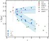 |
Fig. 22 Compilation of size measurements at different redshifts for a number of different studies. First, in blue we show the measurements of this paper. Circles are taken from the GALFIT effective radius, and the triangles and inverted triangles are from |

9. Summary
We studied the evolution in the sizes of star-forming galaxies obtained from a detailed analysis of ~1200 galaxies with 2 <z< 4.5 and stellar masses 9.5 < log (M⋆) < 11.5 in the VIMOS Ultra Deep Survey. We used two different methods to compute sizes: a parametric profile fitting using the GALFIT tool to derive the effective radius re,circ, and we defined and used a non-parametric size measurements based on the area defined as enclosing 100% of the measured flux of a galaxy above a given surface brightness threshold, . While the former makes a strong hypothesis on the symmetry of a galaxy shape, the latter can be applied to galaxies with irregular and asymmetric morphology.
Our results on size measurements can be summarized as follows:
-
The total size of a galaxy was observed to remain approximately constant with a radius
 kpc over the redshift range 2 <z< 4.5, while the effective radius re,circ decreases from ~2 kpc at z ~ 2 to ~1 kpc at z ~ 4.5. The evolution of galaxy sizes is therefore drastically different when using parametric methods with a symmetry prior or a non-parametric method with no a priori assumption of symmetry. This difference between the total radius and the effective radius is more important at the highest redshifts, with a factor ~2 difference at z ~ 4, probably because of the increasing fraction of irregularly shaped galaxies.
 -
A large scatter in galaxy sizes was observed at all redshifts. We observed galaxies as large as ~11 kpc (total extent) out to z = 4.5.
-
The projected luminosity density of galaxies is higher at the highest redshifts. Using stacking analysis and individual measurements, we found that the light concentration of galaxies is ~20% higher at z ~ 4 than at z ~ 2.
-
On average, larger SFGs have higher stellar masses, SFRs and stellar mass densities.
-
These correlations between size and physical properties depend on the size measurement method. We found a stronger correlation between sizes and star-formation rates for
than for re,circ while it was of similar strength when the stellar mass-size relations were considered.
The results presented in this paper on a sample of star-forming galaxies observed 10.5 to 12.5 Gyr ago and 0.5 Gyr after the end of reionization at z ~ 6 emphasize the diversity of galaxy size properties at a time of intense galaxy assembly. The observation of galaxies with total sizes ranging from less than 1 kpc to ~10 kpc seems to require that several different processes drive mass assembly, and may represent different snapshots in the early life history of the dominant population of galaxies at these redshifts.
More detailed investigations connecting size and morphology analyses to different spectral properties from the UV (e.g., Ly-α emission, β-slope) to the optical domain are needed to further understand the diversity of sizes in the early phases of galaxy assembly (Ribeiro et al., in preparation).
Future observations with next-generation facilities such as the James Webb Space Telescope and extremely large telescopes will be necessary to investigate the nature of large and irregular galaxies at these high redshifts in detail and well into the reionization epoch.
Acknowledgments
This work is supported by funding from the European Research Council Advanced Grant ERC–2010–AdG–268107–EARLY and by INAF Grants PRIN 2010, PRIN 2012 and PICS 2013. This work is based on data products made available at the CESAM data center, Laboratoire d’Astrophysique de Marseille. This work partly uses observations obtained with MegaPrime/MegaCam, a joint project of CFHT and CEA/DAPNIA, at the Canada-France-Hawaii Telescope (CFHT) which is operated by the National Research Council (NRC) of Canada, the Institut National des Sciences de l’Univers of the Centre National de la Recherche Scientifique (CNRS) of France, and the University of Hawaii. This work is based in part on data products produced at TERAPIX and the Canadian Astronomy Data Centre as part of the Canada-France-Hawaii Telescope Legacy Survey, a collaborative project of NRC and CNRS.
References
- Akiyama, M., Minowa, Y., Kobayashi, N., et al. 2008, ApJS, 175, 1 [NASA ADS] [CrossRef] [Google Scholar]
- Arnouts, S., Cristiani, S., Moscardini, L., et al. 1999, MNRAS, 310, 540 [NASA ADS] [CrossRef] [Google Scholar]
- Bershady, M. A., Jangren, A., & Conselice, C. J. 2000, AJ, 119, 2645 [NASA ADS] [CrossRef] [Google Scholar]
- Bertin, E., & Arnouts, S. 1996, A&AS, 117, 393 [NASA ADS] [CrossRef] [EDP Sciences] [Google Scholar]
- Bouwens, R., Broadhurst, T., & Illingworth, G. 2003, ApJ, 593, 640 [NASA ADS] [CrossRef] [Google Scholar]
- Bouwens, R. J., Illingworth, G. D., Blakeslee, J. P., Broadhurst, T. J., & Franx, M. 2004, ApJ, 611, L1 [NASA ADS] [CrossRef] [Google Scholar]
- Bouwens, R. J., Illingworth, G. D., Oesch, P. A., et al. 2015, ApJ, 803, 34 [NASA ADS] [CrossRef] [Google Scholar]
- Bruce, V. A., Dunlop, J. S., Cirasuolo, M., et al. 2012, MNRAS, 427, 1666 [NASA ADS] [CrossRef] [Google Scholar]
- Bruzual, G., & Charlot, S. 2003, MNRAS, 344, 1000 [NASA ADS] [CrossRef] [Google Scholar]
- Buitrago, F., Trujillo, I., Conselice, C. J., & Häußler, B. 2013, MNRAS, 428, 1460 [NASA ADS] [CrossRef] [Google Scholar]
- Calzetti, D., Armus, L., Bohlin, R. C., et al. 2000, ApJ, 533, 682 [NASA ADS] [CrossRef] [Google Scholar]
- Capak, P., Aussel, H., Ajiki, M., et al. 2007, ApJS, 172, 99 [NASA ADS] [CrossRef] [Google Scholar]
- Cassata, P., Giavalisco, M., Guo, Y., et al. 2010, ApJ, 714, L79 [NASA ADS] [CrossRef] [Google Scholar]
- Cassata, P., Giavalisco, M., Williams, C. C., et al. 2013, ApJ, 775, 106 [NASA ADS] [CrossRef] [Google Scholar]
- Chabrier, G. 2003, ApJ, 586, L133 [NASA ADS] [CrossRef] [Google Scholar]
- Ciotti, L., & Bertin, G. 1999, A&A, 352, 447 [NASA ADS] [Google Scholar]
- Conselice, C. J., & Arnold, J. 2009, MNRAS, 397, 208 [NASA ADS] [CrossRef] [Google Scholar]
- Curtis-Lake, E., McLure, R. J., Dunlop, J. S., et al. 2016, MNRAS, 457, 440 [NASA ADS] [CrossRef] [Google Scholar]
- Daddi, E., Renzini, A., Pirzkal, N., et al. 2005, ApJ, 626, 680 [NASA ADS] [CrossRef] [Google Scholar]
- Delgado-Serrano, R., Hammer, F., Yang, Y. B., et al. 2010, A&A, 509, A78 [NASA ADS] [CrossRef] [EDP Sciences] [Google Scholar]
- Elmegreen, D. M., Elmegreen, B. G., Ravindranath, S., & Coe, D. A. 2007, ApJ, 658, 763 [NASA ADS] [CrossRef] [Google Scholar]
- Elmegreen, B. G., Elmegreen, D. M., Fernandez, M. X., & Lemonias, J. J. 2009, ApJ, 692, 12 [NASA ADS] [CrossRef] [Google Scholar]
- Ferguson, H. C., Dickinson, M., Giavalisco, M., et al. 2004, ApJ, 600, L107 [NASA ADS] [CrossRef] [Google Scholar]
- Franx, M., van Dokkum, P. G., Schreiber, N. M. F., et al. 2008, ApJ, 688, 770 [NASA ADS] [CrossRef] [Google Scholar]
- Garilli, B., Fumana, M., Franzetti, P., et al. 2010, PASP, 122, 827 [NASA ADS] [CrossRef] [Google Scholar]
- Giavalisco, M., Livio, M., Bohlin, R. C., Macchetto, F. D., & Stecher, T. P. 1996, AJ, 112, 369 [NASA ADS] [CrossRef] [Google Scholar]
- Giavalisco, M., Ferguson, H. C., Koekemoer, A. M., et al. 2004, ApJ, 600, L93 [NASA ADS] [CrossRef] [Google Scholar]
- Grazian, A., Castellano, M., Fontana, A., et al. 2012, A&A, 547, A51 [NASA ADS] [CrossRef] [EDP Sciences] [Google Scholar]
- Grogin, N. A., Kocevski, D. D., Faber, S. M., et al. 2011, ApJS, 197, 35 [NASA ADS] [CrossRef] [Google Scholar]
- Guo, Y., Ferguson, H. C., Bell, E. F., et al. 2015, ApJ, 800, 39 [NASA ADS] [CrossRef] [Google Scholar]
- Hathi, N. P., Malhotra, S., & Rhoads, J. E. 2008, ApJ, 673, 686 [NASA ADS] [CrossRef] [Google Scholar]
- Holwerda, B. W., Bouwens, R., Oesch, P., et al. 2015, ApJ, 808, 6 [NASA ADS] [CrossRef] [Google Scholar]
- Huang, K.-H., Ferguson, H. C., Ravindranath, S., & Su, J. 2013, ApJ, 765, 68 [NASA ADS] [CrossRef] [Google Scholar]
- Huertas-Company, M., Pérez-González, P. G., Mei, S., et al. 2015, ApJ, 809, 95 [NASA ADS] [CrossRef] [Google Scholar]
- Ichikawa, T., Kajisawa, M., & Akhlaghi, M. 2012, MNRAS, 422, 1014 [NASA ADS] [CrossRef] [Google Scholar]
- Ilbert, O., Arnouts, S., McCracken, H. J., et al. 2006, A&A, 457, 841 [NASA ADS] [CrossRef] [EDP Sciences] [Google Scholar]
- Ilbert, O., Salvato, M., Le Floc’h, E., et al. 2010, ApJ, 709, 644 [NASA ADS] [CrossRef] [Google Scholar]
- Ilbert, O., McCracken, H. J., Le Fèvre, O., et al. 2013, A&A, 556, A55 [NASA ADS] [CrossRef] [EDP Sciences] [Google Scholar]
- Jiang, L., Egami, E., Fan, X., et al. 2013, ApJ, 773, 153 [NASA ADS] [CrossRef] [Google Scholar]
- Kawamata, R., Ishigaki, M., Shimasaku, K., Oguri, M., & Ouchi, M. 2015, ApJ, 804, 103 [NASA ADS] [CrossRef] [Google Scholar]
- Koekemoer, A. M., Aussel, H., Calzetti, D., et al. 2007, ApJS, 172, 196 [NASA ADS] [CrossRef] [Google Scholar]
- Koekemoer, A. M., Faber, S. M., Ferguson, H. C., et al. 2011, ApJS, 197, 36 [NASA ADS] [CrossRef] [Google Scholar]
- Law, D. R., Steidel, C. C., Erb, D. K., et al. 2007, ApJ, 656, 1 [NASA ADS] [CrossRef] [Google Scholar]
- Le Fèvre, O., Tasca, L. A. M., Cassata, P., et al. 2015, A&A, 576, A79 [NASA ADS] [CrossRef] [EDP Sciences] [Google Scholar]
- Lubin, L. M., & Sandage, A. 2001, AJ, 122, 1084 [Google Scholar]
- McCracken, H. J., Milvang-Jensen, B., Dunlop, J., et al. 2012, A&A, 544, A156 [NASA ADS] [CrossRef] [EDP Sciences] [Google Scholar]
- Morishita, T., Ichikawa, T., & Kajisawa, M. 2014, ApJ, 785, 18 [NASA ADS] [CrossRef] [Google Scholar]
- Mortlock, A., Conselice, C. J., Hartley, W. G., et al. 2013, MNRAS, 433, 1185 [NASA ADS] [CrossRef] [Google Scholar]
- Mosleh, M., Williams, R. J., Franx, M., & Kriek, M. 2011, ApJ, 727, 5 [NASA ADS] [CrossRef] [Google Scholar]
- Mosleh, M., Williams, R. J., Franx, M., et al. 2012, ApJ, 756, L12 [NASA ADS] [CrossRef] [Google Scholar]
- Nelson, E. J., van Dokkum, P. G., Momcheva, I., et al. 2013, ApJ, 763, L16 [NASA ADS] [CrossRef] [Google Scholar]
- Nelson, E. J., van Dokkum, P. G., Förster Schreiber, N. M., et al. 2015, ApJ submitted [arXiv:1507.03999] [Google Scholar]
- Oesch, P. A., Bouwens, R. J., Carollo, C. M., et al. 2010, ApJ, 709, L21 [NASA ADS] [CrossRef] [Google Scholar]
- Ono, Y., Ouchi, M., Curtis-Lake, E., et al. 2013, ApJ, 777, 155 [NASA ADS] [CrossRef] [Google Scholar]
- Pearson, K. 1896, Phil. Trans. R. Soc. Lond. Ser. A, 187, 253 [Google Scholar]
- Peng, C. Y., Ho, L. C., Impey, C. D., & Rix, H.-W. 2002, AJ, 124, 266 [NASA ADS] [CrossRef] [Google Scholar]
- Peng, C. Y., Ho, L. C., Impey, C. D., & Rix, H.-W. 2010, AJ, 139, 2097 [NASA ADS] [CrossRef] [Google Scholar]
- Petrosian, V. 1976, ApJ, 209, L1 [NASA ADS] [CrossRef] [Google Scholar]
- Ravindranath, S., Ferguson, H. C., Conselice, C., et al. 2004, ApJ, 604, L9 [NASA ADS] [CrossRef] [Google Scholar]
- Ravindranath, S., Giavalisco, M., Ferguson, H. C., et al. 2006, ApJ, 652, 963 [NASA ADS] [CrossRef] [Google Scholar]
- Reddy, N. A., & Steidel, C. C. 2009, ApJ, 692, 778 [NASA ADS] [CrossRef] [Google Scholar]
- Rhodes, J. D., Massey, R. J., Albert, J., et al. 2007, ApJS, 172, 203 [NASA ADS] [CrossRef] [Google Scholar]
- Rix, H.-W., Barden, M., Beckwith, S. V. W., et al. 2004, ApJS, 152, 163 [NASA ADS] [CrossRef] [Google Scholar]
- Scodeggio, M., Franzetti, P., Garilli, B., et al. 2005, PASP, 117, 1284 [NASA ADS] [CrossRef] [Google Scholar]
- Scoville, N., Abraham, R. G., Aussel, H., et al. 2007, ApJS, 172, 38 [NASA ADS] [CrossRef] [Google Scholar]
- Sersic, J. L. 1968, Atlas de galaxias australes (Cordoba, Argentina: Observatorio Astronomico) [Google Scholar]
- Shibuya, T., Ouchi, M., & Harikane, Y. 2015, ApJS, 219, 15 [NASA ADS] [CrossRef] [Google Scholar]
- Simard, L., Koo, D. C., Faber, S. M., et al. 1999, ApJ, 519, 563 [NASA ADS] [CrossRef] [Google Scholar]
- Steidel, C. C., Adelberger, K. L., Giavalisco, M., Dickinson, M., & Pettini, M. 1999, ApJ, 519, 1 [NASA ADS] [CrossRef] [Google Scholar]
- Stott, J. P., Sobral, D., Smail, I., et al. 2013, MNRAS, 430, 1158 [NASA ADS] [CrossRef] [Google Scholar]
- Straatman, C. M. S., Labbé, I., Spitler, L. R., et al. 2015, ApJ, 808, L29 [NASA ADS] [CrossRef] [Google Scholar]
- Stringer, M. J., Shankar, F., Novak, G. S., et al. 2014, MNRAS, 441, 1570 [NASA ADS] [CrossRef] [Google Scholar]
- Tacchella, S., Dekel, A., Carollo, C. M., et al. 2016, MNRAS, 458, 242 [NASA ADS] [CrossRef] [Google Scholar]
- Talia, M., Cimatti, A., Mignoli, M., et al. 2014, A&A, 562, A113 [NASA ADS] [CrossRef] [EDP Sciences] [Google Scholar]
- Tasca, L. A. M., Kneib, J.-P., Iovino, A., et al. 2009, A&A, 503, 379 [NASA ADS] [CrossRef] [EDP Sciences] [Google Scholar]
- Tasca, L. A. M., Le Fèvre, O., Hathi, N. P., et al. 2015, A&A, 581, A54 [NASA ADS] [CrossRef] [EDP Sciences] [Google Scholar]
- Thomas, R., Le Fèvre, O., Cassata, P., et al. 2014, A&A, accepted [arXiv:1411.5692] [Google Scholar]
- Thomas, R., Le Fèvre, O., Scodeggio, M., et al. 2016, A&A, submitted [arXiv:1602.01841], [Google Scholar]
- Tolman, R. C. 1930, PNAS, 16, 511 [Google Scholar]
- Trujillo, I., Förster Schreiber, N. M., Rudnick, G., et al. 2006, ApJ, 650, 18 [NASA ADS] [CrossRef] [Google Scholar]
- van der Wel, A., Franx, M., van Dokkum, P. G., et al. 2014, ApJ, 788, 28 [NASA ADS] [CrossRef] [Google Scholar]
- Williams, R. J., Quadri, R. F., Franx, M., et al. 2010, ApJ, 713, 738 [NASA ADS] [CrossRef] [Google Scholar]
- Wuyts, S., Förster Schreiber, N. M., van der Wel, A., et al. 2011, ApJ, 742, 96 [NASA ADS] [CrossRef] [Google Scholar]
- Wuyts, S., Förster Schreiber, N. M., Genzel, R., et al. 2012, ApJ, 753, 114 [NASA ADS] [CrossRef] [Google Scholar]
Appendix A: T100 in simulated galaxies
We used the same set of simulated galaxy images as described in Sect. 3.3 to compute the value of T100 and assess the effect of the noise on the retrieved values. To compute the value of the expected total area, we used the noise-free simulated models, convolved with a PSF, and applied the same thresholding method as explained in Sect. 4. To ensure that we would probe different threshold a random redshift was attributed to each galaxy, which was taken from a uniform distribution between the limits we defined for this paper. This, in practice, translates into mapping the thresholds used in the computation of sizes in real data.
In Fig. A.1 we show the output results from the simulation. Brighter galaxies have larger sizes because more pixels are found above the threshold that we defined. The scatter that we find to increase for smaller galaxies (fainter magnitudes) is explained by the increasing contamination of the sky-connected pixels that
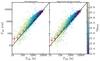 |
Fig. A.1 Results of computing of T100 for a set of 15 000 galaxies. The points are color coded by their input magnitude, and the size of each point is determined by the input re of the GALFIT model. The solid red line denotes the one-to-one relation. The left panel refers to the size measurement without any correction, and the right panel presents the same results, but after applying the same sky correction as described in Sect. 4.6. The large red points represent the median sizes per bin, the error bar in the x-axis represents the bin width, and the y-axis represents the median absolute dispersion of the bin. |
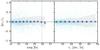 |
Fig. A.2 Variance of the value of re for a set of 15 000 galaxies as a function of input magnitude (left) and effective radii (right). Only galaxies where GALFIT convergence was attained are included in this figure. The large dark blue points represent the median sizes per bin, the error bar in the y-axis is |

are detected close to the galaxy and gain importance with lower the flux of simulated galaxies which produces an overestimation of the galaxy size. Additionally, since we dropped galaxy models on a real background, with potentially other sources in the image area, some large scatter is expected at all magnitudes where sizes are consistently overestimated. The underestimation of galaxy sizes at the largest simulated sources is unexpected. However, since ~90% of the galaxies in our sample have 100 <T100< 2000 pixels we find it a negligible correction with no effect in our findings.
We also applied the same correction method for the contamination of sky-connected pixels, and the results are shown in the right panel of Fig. A.1. It increases somehow the scatter at the lower input sizes and overall approximates the retrieved value from the input one. Being far from perfect, we believe that our sky corrections estimates are good enough for approximating the derived galaxy sizes of our sample.
Appendix B: Concentration parameter
This concentration index is defined as the ratio of the 80% to the 20% curve-of-growth radii within 1.5 times the Petrosian (1976) radius for a parameter η = 0.2: 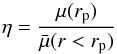 (B.1)where rp is the computed petrosian radius for a given value of η. With that radius we can compute the flux within circular apertures (or elliptical ones) up to which 20% and 80% of the light is contained. But first, it is necessary to define a light center and the axis ratio and position angle so that we can define the elliptical apertures.
To measure these quantities, we first define the barycenter of the galaxy. The intensity centroid is computed as the mean pixel position, averaged by the flux, within the segmentation map:  When we have
  and
and  it is possible to compute the second-order moments of the profile as
![Mathematical equation: \appendix \setcounter{section}{2} \begin{eqnarray} &&\overline{x^2} = \frac{1}{I_{\rm tot}} \sum_{i,j} i^2 \times I_{i,j} - {\bar x}^2 \label{eq:xx} \\[1.5mm] &&\overline{y^2} = \frac{1}{I_{\rm tot}} \sum_{i,j} j^2 \times I_{i,j} - {\bar y}^2 \label{eq:yy}\\[1.5mm] &&\overline{xy} = \frac{1}{I_{\rm tot}} \sum_{i,j} i\times j \times I_{i,j} - {\bar x}{\bar y}\label{eq:xy}. \end{eqnarray}](/articles/aa/full_html/2016/09/aa28249-16/aa28249-16-eq291.png) From there, it is possible to show that (see Bertin & Arnouts 1996)
From there, it is possible to show that (see Bertin & Arnouts 1996)  (B.7)Which is then corrected according to the quadrant it refers to in order to span the entire range from −90 to 90 degrees. It is also possible to directly define the semi-major and semi-minor axis
of the corresponding ellipse as  which in turns facilitates computing q = b/a.
Finally, we can compute the total flux within an elliptical aperture defined by the shape parameters above and a semi-major axis of 1.5rp. From there, we iterate over different apertures with an increasing major-axis to define the radius enclosing 20% and 80% of the total flux defined before. When we have those values, it is straightforward to use Eq. (21) to compute the light concentration of the object.
Figure B.1 confirms that for the same sample defined in this paper, the standard light concentration measurement yields different results and trends. This is most likely because using the elliptical apertures fails to give a actual insight onto how concentrated is the light inside a galaxy that is highly irregular.
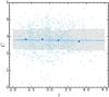 |
Fig. B.1 Redshift dependence of the standard concentration measurement described in this section. The symbols and regions have the same meaning as in Fig. 18. |
All Tables
Best-fit slope and normalization factor for equation log (r) = αrlog (1 + z) + βr for the different size estimates used throughout the paper.
All Figures
|
Fig. 1 Number of galaxies per redshift bin for the entire VUDS sample considering all galaxies with a redshift measurement in light gray and those with a redshift reliability flag corresponding to a >75% certainty in dark gray. In blue we present the distribution for the COSMOS + ECDFS, stellar mass selected and 2 <z< 4.5 sample (all flags in light blue and reliable flags in darker blue). Our results are based on the darker blue histogram, which contains 1242 galaxies. |
| In the text | |
|
Fig. 2 Range in stellar masses and SFRs for the sample studied here. In each panel, the light gray points refer to the entire VUDS sample in each redshift bin. The colored points represent each of the 1242 galaxies in the selected stellar mass range that have reliable spectroscopic flags (correct redshift probability of >75%, see text for more details). |
| In the text | |
|
Fig. 3 NUVrJ diagram (Ilbert et al. 2010, 2013) for the sample studied here in different redshift bins. In each panel the colors have the same meaning as in Fig. 2. |
| In the text | |
|
Fig. 4 Comparison of size measurements derived with GALFIT for a subset of 153 (118) VUDS galaxies at 2 <z< 4.5 with available F814W and F160W (F125W) images from CANDELS. Results are split into two bands: F160W in the top panel and F125W in the bottom panel. Circles and squares refer to COSMOS and ECDFS respectively. The dashed black line shows where the two radii are equal. The symbols are color coded according to their spectroscopic redshift and the mapping is shown in the colorbar at the top of the plots. Fewer galaxies are available in the J-band comparison because there are no such data available in ECDFS. |
| In the text | |
|
Fig. 5 Measured sizes as a function of wavelength for galaxies with log 10(M⋆) > 9.5 at 2 <z< 4.5 in the COSMOS field. Different symbols correspond to different surveys (symbol coding in the bottom panel) and different colors to different observed bands (color coding in the top panel). Each point represents the size of a given galaxy at the rest-frame wavelength of the pivot of the filter. |
| In the text | |
|
Fig. 6 Size distribution for different redshift bins. The vertical dashed line indicates the median value for each bin. The black line is the fit of the distribution using a normal function in log space. |
| In the text | |
|
Fig. 7 Size evolution with redshift. Each galaxy with a good size measurement is plotted with a small blue point (squares for redshift confidence 2 and 9, circles for 3 and 4). The median values (in redshift and size for each bin) and respective error ( |
| In the text | |
|
Fig. 8 Illustration of the size measurement process for VUDS 510799304 at z = 2.4281. From left to right: (1) the original F814W image from COSMOS (Koekemoer et al. 2007). (2) The same image after smoothing by a Gaussian kernel of 1 pixel width and extending over four times the width. This kernel ensures an improvement in signal to noise for low surface brightness levels while preventing a significant boost of noisy pixels, which would incidentally increase the measured radius if the kernel were too large. (3) The segmentation map obtained after running the detection algorithm including all pixels greater than kσ. (4) The selection of the target galaxy. All panels have 1.77′′by 1.77′′and the orange circle has a radius of 0.5′′. The total size is computed from the number of pixels in the last panel. |
| In the text | |
|
Fig. 9 F814W imaging in COSMOS (Koekemoer et al. 2007) and CANDELS (when available, Koekemoer et al. 2011) of the measured sizes for three galaxies in each of four increasing redshift bins from z ~ 2.4 to z ~ 4.1 (top to bottom) in our sample. The green contours show a smoothed version of the segmentation map of the galaxy at the defined threshold, which translates into T100 from Eq. (6) measured at kp = 1.0. The black ellipses are constructed from the values of re,b/a and θPA derived from GALFIT for those galaxies. The parametric and symmetric 2D profile fitting with GALFIT fails to properly account for the complex irregular morphology when deriving the size of galaxies at these redshifts, while the non-parametric method presented in this paper is able to derive more realistic sizes. |
| In the text | |
|
Fig. 10 Value of k as a function of redshift for different choices of kp. The vertical dotted line shoes the upper redshift limit we assume in this paper. The black solid line shows the depth limit above which the noise correction is larger than 100 pixels. |
| In the text | |
|
Fig. 11 Comparison of |
| In the text | |
|
Fig. 12 F814W (in blue) and F160W (in red) imaging in CANDELS (Koekemoer et al. 2011) of six example galaxies in VUDS. The green contours show the isophote used to derive |
| In the text | |
|
Fig. 13 Total size distribution for different redshift bins. The vertical dotted line indicates the median value for each bin. The black line is the fit of the distribution using a normal function in log space. |
| In the text | |
|
Fig. 14 Comparison of the two size estimates. With dark blue points we show the comparison to |
| In the text | |
|
Fig. 15 Total size evolution with redshift. Each galaxy is plotted with a small blue point (squares for redshift confidence 2 and 9, circles for 3 and 4). The median values and respective error ( |
| In the text | |
|
Fig. 16 Total size measurements defined at different values of kp that correspond to different luminosity thresholds at z = 2. From top to bottom, the colored circles correspond to kp = 0.8,1.0,1.2,1.5, and 2.0. The color coding is the same as in Fig. 10. |
| In the text | |
|
Fig. 17 Normalized surface luminosity profiles of the median stacked F814W band images of galaxies in our sample at four different redshift bins (normalized at r = 0.3 kpc). The width of each profile encodes the surface luminosity error. This profile comparison shows the increased light concentration at higher redshifts. |
| In the text | |
|
Fig. 18 Evolution of light concentration in galaxies computed from the ratio of the non-parametric radii enclosing 80% and 20% of the total flux, as defined in Sect. 4. The solid line is a linear fit to all the small blue points. Each galaxy is plotted with a small blue point (squares for redshift confidence 2 and 9, circles for 3 and 4). The median values and respective error ( |
| In the text | |
|
Fig. 19 Slope of the evolution of PSF corrected galaxy sizes as a function of the flux level considered. The light colored symbols correspond to the slope computed from sky-corrected |
| In the text | |
|
Fig. 20 Correlation of the measured galaxy sizes with parameters derived from GOSSIP+ SED fitting for our stellar-mass-selected sample (using the stellar masses derived with GOSSIP + and Eq. (1)). Only galaxies with good and excellent spectrophotometric fits are included. From top to bottom we show the stellar mass, SFR, age, and dust extinction. In the right panels we show the results for GALFIT derived re,circ and in the left panels we show the results for our value of |
| In the text | |
|
Fig. 21 Stellar mass surface density as a function of stellar mass. In the right panels we show the results for GALFIT derived re,circ and in the left panels we show the results for our value of |
| In the text | |
|
Fig. 22 Compilation of size measurements at different redshifts for a number of different studies. First, in blue we show the measurements of this paper. Circles are taken from the GALFIT effective radius, and the triangles and inverted triangles are from |
| In the text | |
|
Fig. A.1 Results of computing of T100 for a set of 15 000 galaxies. The points are color coded by their input magnitude, and the size of each point is determined by the input re of the GALFIT model. The solid red line denotes the one-to-one relation. The left panel refers to the size measurement without any correction, and the right panel presents the same results, but after applying the same sky correction as described in Sect. 4.6. The large red points represent the median sizes per bin, the error bar in the x-axis represents the bin width, and the y-axis represents the median absolute dispersion of the bin. |
| In the text | |
|
Fig. A.2 Variance of the value of re for a set of 15 000 galaxies as a function of input magnitude (left) and effective radii (right). Only galaxies where GALFIT convergence was attained are included in this figure. The large dark blue points represent the median sizes per bin, the error bar in the y-axis is |
| In the text | |
|
Fig. B.1 Redshift dependence of the standard concentration measurement described in this section. The symbols and regions have the same meaning as in Fig. 18. |
| In the text | |
Current usage metrics show cumulative count of Article Views (full-text article views including HTML views, PDF and ePub downloads, according to the available data) and Abstracts Views on Vision4Press platform.
Data correspond to usage on the plateform after 2015. The current usage metrics is available 48-96 hours after online publication and is updated daily on week days.
Initial download of the metrics may take a while.