The VIMOS Ultra-Deep Survey: Emerging from the dark, a massive proto-cluster at z ~ 4.57

B. C. Lemaux; O. Le Fèvre; O. Cucciati; B. Ribeiro; L. A. M. Tasca; G. Zamorani; O. Ilbert; R. Thomas; S. Bardelli; P. Cassata; N. P. Hathi; J. Pforr; V. Smolčić; I. Delvecchio; M. Novak; S. Berta; H. J. McCracken; A. Koekemoer; R. Amorín; B. Garilli; D. Maccagni; D. Schaerer; E. Zucca

doi:10.1051/0004-6361/201730870

Home

All issues

Volume 615 (July 2018)

A&A, 615 (2018) A77

Full HTML

Open Access

Issue		A&A Volume 615, July 2018


Article Number		A77
Number of page(s)		27
Section		Extragalactic astronomy
DOI		https://doi.org/10.1051/0004-6361/201730870
Published online		17 July 2018

A&A 615, A77 (2018)

The VIMOS Ultra-Deep Survey: Emerging from the dark, a massive proto-cluster at z ~ 4.57^★

B. C. Lemaux¹^,2, O. Le Fèvre², O. Cucciati³^,6, B. Ribeiro², L. A. M. Tasca², G. Zamorani³, O. Ilbert², R. Thomas²^,4, S. Bardelli³, P. Cassata⁴, N. P. Hathi²^,11, J. Pforr²^,12, V. Smolčić⁷, I. Delvecchio⁷, M. Novak⁷, S. Berta⁷^,8^,★★, H. J. McCracken⁹^,10, A. Koekemoer¹¹, R. Amorín¹³^,14, B. Garilli⁵, D. Maccagni⁵, D. Schaerer¹⁵^,16 and E. Zucca³

¹ Department of Physics, University of California, 1 Shields Ave, Davis, CA 95616, USA
e-mail: bclemaux@ucdavis.edu
² Aix-Marseille Université, CNRS, LAM (Laboratoire d’Astrophysique de Marseille), UMR 7326, 13388 Marseille, France
³ INAF – Osservatorio Astronomico di Bologna, via Gobetti 93/3, 40129 Bologna, Italy
⁴ Instituto de Física y Astronomía, Facultad de Ciencias, Universidad de Valparaíso, Gran Bretañ a 1111, Playa Ancha, Valparaíso, Chile
⁵ INAF – IASF, via Bassini 15, 20133 Milano, Italy
⁶ University of Bologna, Department of Physics and Astronomy (DIFA), viale Berti Pichat 6/2, 40127 Bologna, Italy
⁷ Department of Physics, Faculty of Science, University of Zagreb, Bijenička cesta 32, 10000 Zagreb, Croatia
⁸ Max-Planck-Institut für extraterrestrische Physik (MPE), Postfach 1312, 85741 Garching, Germany
⁹ Sorbonne Université, UPMC Université Paris 6 et CNRS, UMR 7095, Institut d’Astrophysique de Paris, 98 bis Boulevard Arago, 75014 Paris, France
¹⁰ Institut d’Astrophysique de Paris, UMR 7095 CNRS, Université Pierre et Marie Curie, 98 bis Boulevard Arago, 75014 Paris, France
¹¹ Space Telescope Science Institute, 3700 San Martin Drive, Baltimore, MD 21218, USA
¹² European Space Agency, ESA/ESTEC, Keplerlaan 1, 22001 AZ Noordwijk, The Netherlands
¹³ Cavendish Laboratory, University of Cambridge, 19 J.J. Thomson Ave, Cambridge CB30HE, UK
¹⁴ Kavli Institute for Cosmology, University of Cambridge, Madingley Road, Cambridge CB30HA, UK
¹⁵ Department of Astronomy, University of Geneva, ch. d’Écogia 16, 1290 Versoix, Switzerland
¹⁶ Observatoire de Genève, 51 ch. des Maillettes, 1290 Versoix, Switzerland

Received: 25 March 2017
Accepted: 3 January 2018

Abstract

Using spectroscopic observations taken for the Visible Multi-Object Spectrograph (VIMOS) Ultra-Deep Survey (VUDS) we report here on the discovery of PCl J1001+0220, a massive proto-cluster of galaxies located at z_spec ~ 4.57 in the COSMOS field. With nine spectroscopic members, the proto-cluster was initially detected as a ~12σ spectroscopic overdensity of typical star-forming galaxies in the blind spectroscopic survey of the early universe (2 < z ≲ 6) performed by VUDS. It was further mapped using a new technique developed which statistically combines spectroscopic and photometric redshifts, the latter derived from a recent compilation of incredibly deep multi-band imaging performed on the COSMOS field. Through various methods, the descendant mass of PCl J1001+0220 is estimated to be log (M_h/M_⊙)_z=0 ~ 14.5–15 with a large amount of mass apparently already in place at z ~ 4.57. An exhaustive comparison was made between the properties of various spectroscopic and photometric member samples and matched samples of galaxies inhabiting less dense environments at the same redshifts. Tentative evidence is found for a fractional excess of older galaxies more massive in their stellar content amongst the member samples relative to the coeval field, an observation which suggests the pervasive early onset of vigorous star formation for proto-cluster galaxies. No evidence is found for the differences in the star formation rates (SFRs) of member and coeval field galaxies either through estimating by means of the rest-frame ultraviolet or through separately stacking extremely deep Very Large Array 3 GHz imaging for both samples. Additionally, no evidence for pervasive strong active galactic nuclei (AGN) activity is observed in either environment. Analysis of Hubble Space Telescope images of both sets of galaxies as well as their immediate surroundings provides weak evidence for an elevated incidence of galaxy–galaxy interaction within the bounds of the proto-cluster. The stacked and individual spectral properties of the two samples are compared, with a definite suppression of Lyα seen in the average member galaxy relative to the coeval field (f_esc, _Lyα = 1.8_−1.7^+0.3% and 4.0_−0.8^+1.0%, respectively). This observation along with other lines of evidence leads us to infer the possible presence of a large, cool, diffuse medium within the proto-cluster environment evocative of a nascent intracluster medium forming in the early universe.

Key words: galaxies: evolution / galaxies: clusters: general / galaxies: high-redshift / techniques: spectroscopic / techniques: photometric

^★

Based on data obtained with the European Southern Observatory Very Large Telescope, Paranal, Chile, under Large Program 185.A-0791.

^★★

Visiting scientist.

© ESO 2018

Open Access article, published by EDP Sciences, under the terms of the Creative Commons Attribution License (http://creativecommons.org/licenses/by/4.0;), which permits unrestricted use, distribution, and reproduction in any medium, provided the original work is properly cited.

1 Introduction

The last decade and a half has seen a revolution in the study of overdensities in the early Universe. While the study and careful characterization of large associations of galaxies in the local Universe has been possible for nearly a century, and in the intermediate redshift Universe for a significant fraction of that time (e.g., Shapley & Ames 1926; Shapley 1930; Zwicky 1937; Abell 1958; Zwicky et al. 1961), the study of their progenitors presented several practical problems which have prevented their study until relatively recently. The primary problem, inherent to the study of nearly all galaxy populations in the early Universe, is the extreme apparent faintness of galaxy populations at these distances. While some phenomena exist in the early Universe, such as quasars or radio galaxies, which are so powerful and intrinsically bright that they have been able to serve as beacons to early searches near the epoch of H I reionization (z ~ 5.5–10, Becker et al. 2001, 2015; Planck Collaboration XIII 2016), the bulk of the galaxy population residing in the early Universe does not contain such phenomena (Miley & De Breuck 2008; Ouchi et al. 2008; Lemaux et al. 2014b; Ueda et al. 2014; Talia et al. 2017). As such, the first searches for these more typical primeval galaxies were largely doomed to failure (Davis & Wilkinson 1974; Partridge 1974; Pritchet & Hartwick 1987; Parkes et al. 1994). It was not until the advent of the 10m-class ground-based telescopes largely used in conjunction with the Hubble Space Telescope (HST) that the prospect of detecting and characterizing moderate samples of such galaxies became even remotely feasible (e.g., Steidel et al. 1999; Shapley et al. 2003; Giavalisco et al. 2004; Stanway et al. 2004; Malhotra & Rhoads 2004; Malhotra et al. 2005; Vanzella et al. 2005, Le Fèvre et al. 2005). With this, the prospect of finding and characterizing analogs of the progenitors of the massive clusters and superclusters of galaxies scattered throughout the local Universe began to come within the realm of possibility.

However, other issues remained. At least in the local and intermediate-redshift Universe (z≲1.5), massive overdensities of galaxies are relatively rare (Piffaretti et al. 2011; Campanelli et al. 2012) requiring searches over large swaths of the sky. While redshifts derived from imaging data alone can, with careful calibration, be used to select relatively pure and complete samples of overdensities at these redshifts, and while en masse small-scale clustering of at least certain types of populations may be reproducible with carefully crafted photometric redshift schemes (e.g., Ménard et al. 2013; Schmidt et al. 2013; Aragon-Calvo et al. 2015), the internal structure and dynamics of such overdensities are impossible to characterize on an individual basis without considerable investment of telescope time to obtain spectroscopic followup observations (see e.g., Oke et al. 1998; Dressler et al. 1999; Halliday et al. 2004; Gal et al. 2008; Dressler et al. 2013 and references therein). As both of these issues are potentially exacerbated at higher redshift (z≳1.5), searches for overdensities at such redshifts were potentially required to both be larger and to compensate for larger levels of impurity and incompleteness than their lower redshift analogues. The large amounts of telescope time necessary to detect and confirm even the most modest number of individual high-redshift galaxies made such large-scale searches prohibitive. Further, the study of galaxy overdensities, clusters, superclusters, and, to a lesser extent, groups of galaxies, in the local and intermediate-redshift Universe takes a somewhat regularized form. Such overdensities are known to contain certain markers that allow them to be detected readily, though with varying degrees of purity and completeness. To some degree, nearly all massive overdensities in the low- to intermediate-redshift Universe are marked by a sequence of bright, redder galaxies (e.g., Gladders & Yee 2005; Ascaso et al. 2014, 2015) and by a hot medium, detectable, at least in principle, in the X-ray through bremsstrahlung emission and at mm/cm wavelengths through the Sunyaev-Zel’dovich effect (e.g., Pierre et al. 2004, 2016; Muchovej et al. 2007; Piffaretti et al. 2011; Hasselfield et al. 2013; Rumbaugh et al. 2013; Clerc et al. 2014; Bleem et al. 2015). Additionally, the main component of the mass of these overdensities typically takes a regular, triaxial shape, which, combined with their immense mass and favorable geometric conditions, allowed for at least some of these overdensities to be detected through weak or strong gravitational lensing (e.g., Paczynski 1987; Soucail et al. 1987; Fort & Mellier 1994; Clowe et al. 1998; Gladders et al. 2003; Jee et al. 2006; Hoekstra et al. 2013; Schrabback et al. 2018). While exceptions exist, it was these signposts that allowed for the success of early systematic searches for such overdensities, even with relatively moderate means. Analogs of the progenitors of these populations do not, however, necessarily share these signposts. The increasingly short time allowed for galaxies to form and evolve, to generate and heat an overarching medium, and for an overdensity to build up even a remote fraction of its eventual total mass, requires that the utility of all the methods mentioned above must necessarily decrease and eventually fail as searches move to higher redshift.

The first searches for high-redshift overdensities, historically termed proto-clusters, attempted to overcome these deficiencies, with considerable success, by utilizing the previously mentioned beacons, quasars, other radio-emitting active galactic nuclei (AGN), and extremely prodigious star-forming galaxies also known as sub-mm galaxies (Ivison et al. 2000; Pentericci et al. 2000; Venemans et al. 2002; Miley et al. 2004; Zheng et al. 2006; Overzier et al. 2008). The initial exploration of the surroundings of such phenomena took the form of large-scale deep narrowband imaging which allowed for the determination of the density of specific types of star-forming galaxies known as Lyman α λ1215.7 Å emitters (LAEs) as searches for such galaxies in this manner were relatively economical in terms of telescope time. Despite the success of these searches, it was not clear that such beacons were a requisite condition for a proto-cluster to form in the early Universe and, if not, whether the proto-clusters found around such phenomena were typical. Further, only preliminary estimates were available of how the clustering of LAEs related to the clustering of galaxies as a whole (e.g., Ouchi et al. 2003), the former being a relatively small subset of the overall population (Schenker et al. 2012; Cassata et al. 2015), which, at least when selected through narrowband imaging, are potentially biased towards specific types of galaxies (e.g., Gawiser et al. 2006; Trainor et al. 2015). While later surveys employed identical techniques to target other recombination lines, such as, for example, the Hα λ6563 Å feature (e.g., Hatch et al. 2011; Matsuda et al. 2011), both these surveys and those of LAEs potentially suffered from lack of spectroscopic confirmation of the presumed features. Though some earlier methods detected and attempted to characterize proto-clusters through the photometric selection of a more representative population of high-redshift galaxies known as Lyman break galaxies (LBGs), the lack of redshift resolution of early LBG selection techniques (Δz ~ 1) meant that only a few such selected overdensities held up to scrutiny (e.g., Steidel et al. 1998).

In recent years, however, searches have begun to shift to large samples of L^* -type galaxies using a variety of different techniques. While systematic spectroscopic characterization is still a luxury, large deep photometricsurveys combined with dedicated spectroscopic followup of interesting patches of the sky, as well as archival searches of compilations of observations, are starting to produce results, with regular, well-defined selection criteria for proto-clusters (Capak et al. 2011b; Chiang et al. 2014; Dey et al. 2016; Wang et al. 2016; Franck & McGaugh 2016a,b; Toshikawa et al. 2016). In addition, contemporary searches are persisting over large regions of the sky using radio or sub-mm galaxies (Wylezalek et al. 2013; Casey et al. 2015; Smolčić et al. 2017a) allowing for a comparison sample to those proto-clusters selected blind to such beacons, crucial to understanding whether or not the presence of such phenomena biases the types of proto-cluster environments found in these searches (see e.g., Hatch et al. 2014). Correspondingly, major advances in the understanding of proto-clusters are coming from the study of both N-body simulations and semi-analytic models (e.g., Chiang et al. 2013; Muldrew et al. 2015; Orsi et al. 2016). Both observations and models are converging on the realization that proto-clusters are extremely large in volume, contain diverse galaxy populations, and are more or less readily detectable depending on the galaxy population observed. Developing selection criteria applicable to all types of proto-clusters, a precise, well-characterized methodology of defining membership, and a consistent method to construct comparable lower-density galaxy samples, all of which were elusive in earlier searches for proto-clusters due to the inhomogeneity in both the conception of what a proto-cluster is and the observations employed for the search, is crucial to advancing the study of environmentally-driven evolution in the early Universe. With new large-scale deep photometric and spectroscopic surveys imminent, such as those planned with the Large Synaptic Survey Telescope (LSST), Euclid, Hobby-Eberly Telescope Dark Energy Experiment (HETDEX), and Subaru Prime Focus Spectrograph (PFS), all of which capable, in principle, of detecting extremely large numbers of proto-clusters, the need to determine an operational definition of these structures becomes imperative.

The wide-scale detection and careful characterization of high-redshift overdensities is not simply an academic exercise. Many open questions remain regarding the formation and early development in the life of present-day massive clusters and the constituent galaxies which seed them. While several studies of z ~ 1 clusters have placed the formation epoch of the massive red galaxies prevalent in such structures at z_f ~ 3–4 (Rettura et al. 2010; Raichoor et al. 2012; Lemaux et al. 2012; Zeimann et al. 2012), observational evidence of rapidly forming massive galaxies in proto-clusters at these redshifts is sparse. Such activity, if observed, would contain natural pathways not only to form the requisite number of massive quiescent galaxies observed in intermediate-redshift clusters through gas depletion, but also to begin the transfer of baryonic mass away from the constituent galaxies and into the infant intracluster medium (proto-ICM) through merging activity, tidal stripping, stellar feedback, and AGN activity. The inferred presence of a dense medium in the few z ~ 2–3 overdensities where such an investigation has been possible (e.g., Gobat et al. 2011; Cucciati et al. 2014; Lee et al. 2016; Wang et al. 2016; Cai et al. 2017) strongly suggests that the processes by which the earliest (proto-)cluster galaxies are quenched occur coevally with the formation of this medium. The observation of pervasive AGN activity in many high-redshift proto-clusters also suggests a possible mechanism to pre-heat the proto-ICM, a necessary requirement to reproduce observed cluster scaling relations (see e.g., Hilton et al. 2012; Kravtsov & Borgani 2012 and references therein). The large amount of diffuse gas possibly contained within the proto-ICM and in areas surrounding proto-clusters may cause such regions to be the last in the Universe to undergo H I reionization (e.g., Ciardi et al. 2003), though it is also possible that, due to the increased density of star-forming galaxies, they are the first (e.g., Castellano et al. 2016).

In this paper we report on the systematic search for high-redshift overdensities in the Cosmic Evolution Survey (COSMOS; Scoville et al. 2007b) field using new observations from the VIsible Multi-Object Spectrograph (VIMOS; Le Fèvre et al. 2003) taken as part of the VIMOS Ultra-Deep Survey (VUDS; Le Fèvre et al. 2015). These observations were combined with new and archival deep multi-band imaging and used in conjunction with a new density-mapping technique to discover PCl J1001+0220, a massive proto-cluster at z ~ 4.57 emerging just ~250–500 Myr after the canonical end of H I reionization. The structure of the paper is as follows. Section 2 provides an overview of the spectroscopic and imaging data available in the COSMOS field, as well as the derivation of physical parameters of galaxies in our sample, with particular attention paid to observations from the VUDS survey. Section 3 describes the search methodology employed used to discover PCl J1001+0220 and to quantify its statistical overdensity. In Sect. 4 we describe the estimation of the total mass of PCl J1001+0220 and an investigation of the properties of its spectroscopically-confirmed members compared with properties of galaxies inhabiting lower-density environments. Finally, Sect. 5 presents a summary of our results. Throughout this paper all magnitudes, including those in the infrared (IR), are presented in the AB system (Oke & Gunn 1983; Fukugita et al. 1996). All equivalent width (EW) measurements are presented in the rest frame with negative EWs defined as features observed in emission. Unless otherwise noted, distances are given in proper rather than comoving units. We adopt a concordance Λ Cold Dark Matter (Λ CDM) cosmology with H₀ = 70 km s⁻¹ Mpc⁻¹, Ω_Λ = 0.73, and Ω_M = 0.27. While abbreviated for convenience, throughout the paper stellar masses are presented in units of $h_{70}^{- 2} M_{*}$ $h_{70}^{-2} \mathcal{M}_{\ast}$ , star formation rates (SFRs) in units of $h_{70}^{- 2} M_{*}$ $h_{70}^{-2}\,\mathcal{M}_{\ast}$ yr⁻¹, total masses in units of $h_{70}^{- 1} M_{*}$ $h^{-1}_{70}~\mathcal{M}_{\ast}$ , ages in units of $h_{70}^{- 1}$ $h^{-1}_{70}$ Gyr or $h_{70}^{- 1}$ $h^{-1}_{70}$ Myr, absolute magnitudes in units of M_AB + 5log(h₇₀), proper distances and areas in units of $h_{70}^{- 1}$ $h_{70}^{-1}$ kpc/Mpc and $h_{70}^{- 2}$ $h_{70}^{-2}$ kpc²/Mpc², respectively, where h₇₀ ≡ H₀∕70 km⁻¹ s Mpc.

2 Observations

To date, the Cosmic Evolution Survey (COSMOS) field ([α_J2000, δ_J2000] = [10:00:28.6,+02:12:21.0]) is arguably the most well-studied patch of the entire sky. It has been observed at wavelengths which span nearly the entirety of the electromagnetic spectrum, a large fraction of which we utilize in this paper. In Appendix A we summarize the various datasets available in the COSMOS field.

2.1 Spectroscopic data

The primary impetus for the current study comes from the vast spectroscopic data available in the COSMOS field, with a nearly exclusive reliance on recent VIMOS spectroscopic observations taken as part of VUDS. We therefore begin here with a brief discussion of the spectroscopic survey whose data are used for this study.

2.1.1 The VIMOS Ultra-Deep Survey

The observations from which nearly the entirety of our results are derived were drawn from VIMOS observations taken for VUDS, a massive 640-h (~80 night) spectroscopic campaign reaching extreme depths (i′≲25) over 1 □° in COSMOS, the 02h field of the VIMOS Very Large Telescope Deep Survey (VVDS-02h)¹, and the Extended Chandra Deep Field South (E-CDF-S). The design, goals, and survey strategy of VUDS are described in detail in Le Fèvre et al. (2015) and are thus described here only briefly.

The primary goal of the VUDS survey is to measure the spectroscopic redshifts of a large sample of galaxies at redshifts 2≲z≲6. To this end, target selection was performed primarily through photometric redshift cuts, occasionally supplemented with a variety of magnitude and color−color criteria. These selections were used primarily to maximize the number of galaxies with redshifts likely in excess of z≳2 (see discussion in Le Fèvre et al. 2015) and, in the COSMOS field, to complement the largely color-color selected zCOSMOS-Deep sample. This selection has been used to great effect, as a large fraction (72.4%) of the galaxies with secure spectroscopic redshifts (see below) in VUDS-COSMOS are at z > 2. The main novelties of the VUDS observations are the depth of the spectroscopy, the large wavelength coverage that is afforded by the 50 400 s integration time per pointing and per grating with the low-resolution blue and red gratings on VIMOS (R ~230), and the large sky area covered by the survey. The combination of wavelength coverage and depth along with the high redshift of the sample allows not only for spectroscopic confirmation of the LAE galaxies, galaxies which dominate other high-redshift spectroscopic samples, but also for redshift determination from Lyman series and interstellar medium (ISM) absorption in those galaxies that exhibit no or weak emission line features. Thus, the VUDS data allow for a selection of a spectroscopic volume-limited sample of galaxies at redshifts 2≲z≲6, a sample that probes as faint as $~ M_{F U V}^{*}$ ${\sim}M^{\ast}_{FUV}$ at the redshifts of interest for the study presented in this paper (Cassata et al. 2015).

The flagging code for VUDS is discussed in Le Fèvre et al. (2015). For some of the analysis presented in the paper, we adopt spectroscopic flags = X2, X3, & X4, where X = 0–3², for which the probability of the redshift being correct is ≳75% (hereafter “secure spectroscopic redshifts”). For other portions of this paper we will take a statistical approach incorporating the likelihood of each spectroscopic redshift rather than relying on binary logic (see Sect. 3.3). In total, spectra of 4303 unique objects were obtained as part of VUDS in the COSMOS field, with 2687 of those resulting in secure spectroscopic redshifts (a ~60% redshift success rate, a value consistent with that of the full survey). The spectroscopic sampling of VUDS in the COSMOS field is uniform in that no VUDS pointing appreciably overlaps another in the field.

While we could, in principle, use galaxies targeted by VUDS in the other two fields of the survey (VVDS-02h and E-CDF-S), effectively doubling the control sample used in this study, we choose not to for two reasons. The first is that the COSMOS photometry is more varied and, in general, deeper than that of the other two fields. Our lack of need for excess statistical power of the control sample outweighs the potential for adding in any secondary effects due to unseen bias due to inputting different photometry in the spectral energy distribution (SED) fitting procedure. The second and more important reason is that the lack of comparable photometric depth in the other two VUDS fields causes the reconstruction of the density field (see Sect. 3.3), at least at the current level of implementation, to be more suspect for both fields at the redshift of this study (z≳4.5), meaning we cannot robustly discriminate between low- and moderate-density environments at these redshifts. For further discussion of the survey design, observations, reduction, redshift determination, and the properties of the full VUDS sample, see Le Fèvre et al. (2015). See also (Tasca et al. 2017) for the first VUDS data release, which is available through the Centre de donnéeS Astrophysiques de Marseille (CeSAM) database³.

2.1.2 Other spectroscopic data

In order to maximize the effectiveness of our search for overdensities in the region of the COSMOS field covered by VUDS, we additionally drew spectroscopic redshifts from the zCOSMOS-Bright⁴ (Lilly et al. 2007, 2009) and zCOSMOS-Deep (Lilly et al., in prep., Diener et al. 2013, 2015) surveys. Accounting for duplicate objects where a more secure spectroscopic redshift was available from VUDS, a total of 19485 secure spectroscopic redshifts for unique objects are available from zCOSMOS of which 2034 are at z > 2 and only a small percentage (~1%) reach z > 3. A small number of additional redshifts were also taken from Casey et al. (2015), Chiang et al. (2015), and Diener et al. (2015) at z ~ 2.5, all of which were considered secure. While we include mention of the additional redshifts of these surveys here to demonstratethe precision and accuracy of our photometric redshifts (see following section) and to contextualize the main subject of this paper in terms of the full search for overdensities (see Sect. 3.3), it is important to note that none of these galaxies enter into the main portion of the analysis presented in this paper (i.e., 4 ≤ z ≤ 5) and, thus, differential selection effects resulting from different targeting strategies are irrelevant.

The variety of other spectroscopic observations taken across the COSMOS field (see Ilbert et al. 2013 for a review) were not incorporated into this analysis either because they were at redshifts that are too low to be pertinent to this study or the redshifts were not public at the time of publishing. The one exception is the DEep Imaging and Multi-Object Spectrometer (DEIMOS; Faber et al. 2003) campaign undertaken in the COSMOS field by Capak et al. (2011a) targeting luminous galaxies at 4.5 <z < 6.5. However, these observations are offset too far from the main target in this study, the closest slit being located 7.2′ (~3 Mpc) away from the center of our target (see Sect. 3.1). While these observations, which contain a roughly equivalent number of z > 4 galaxies as VUDS-COSMOS, could be, in principle, useful for bolstering the high-redshift (coeval) field sample defined in Sect. 4.2.1 concerns over differential bias between this campaign and that of VUDS far outweigh the gain in sample size. As such, we do not include these observations as part of this study.

2.2 Synthetic model fitting

Despite the high density and immense depth of the spectroscopic coverage in the COSMOS field, the majority of the objects in the field that are detectable to the depth of our imaging data were not targeted with spectroscopy. For these objects, information can only be obtained through fitting to their SEDs in the observed-frame optical/near-infrared (NIR) broadband photometry. For this study we adopt four different forms of SED fitting. The four methods are used in complementary fashion throughout the paper and the results from each method are compared internally expiating any relative bias.

2.2.1 Photometric redshifts

To estimate photometric redshifts for objects with redshifts left unconstrained from spectroscopic observations, we draw from the fitting performed on the most recent version of the COSMOS2015 catalog (v1.3, Laigle et al. 2016) which employs the use of LE PHARE⁵ (Arnouts et al. 1999; Ilbert et al. 2006, 2009) on point-spread function (PSF)-matched photometry from far-ultraviolet (FUV) to [8.0]. Photometric redshifts, used as priors for a second round of fitting and magnitudes, originally estimated from 3′′ apertures, are corrected to total magnitudes following the method of Moutard et al. (2016) and used to derive associated physical quantities, for example, stellar masses, mean luminosity-weighted stellar ages, extinctions, and SFRs. The parameters used for deriving these quantities are identical to those given in Lemaux et al. (2014a) and to those used for the following two methods in this section. For further details on this process as well as the assumptions and parameterization input for the SED-fitting process, see Laigle et al. (2016).

In Fig. 1 we show a comparison of the photometric redshifts derived from the COSMOS2015 catalog with the cut given above and the associated secure spectroscopic redshifts. The normalized median of the absolute deviations, σ_NMAD (Hoaglin et al. 1983), for the full sample (21781 objects) along with the σ_NMAD, the median photo-z offset (Δ_z ∕(1 + z_s)), and the catastrophic outlier rate (|z_p − z_s|∕(1 + z_s) > 0.15; η) for 4 < z_spec < 5 (131 galaxies) are shown in the main panel of Fig. 1. If we instead adopt an alternative approach sometimes used to estimate photometric redshift precision and fit a Gaussian to the (z_phot − z_spec)∕(1 + z_spec) distributions we recover σ_z∕(1+z) = 0.008 and 0.0145 for the full sample and the subsample at 4 < z < 5, respectively.These numbers are consistent with previous estimates of photometric redshift precision in the COSMOS field at similar redshifts (e.g., Smolčić et al. 2017a).

Throughout the paper we conservatively adopt the σ_NMAD estimate as the formal uncertainty on photometric redshifts. This estimate, however, is still likely to be a lower limit to the true spread in the photo-z population selected in this study for the following reasons. As the accuracy and precision of photometric redshifts is a function of magnitude (see e.g., Ilbert et al. 2006, 2009), the difference of more than a magnitude between the median [3.6] magnitude of the spectral sample at 4 < z_spec < 5 and the [3.6]-limited z_phot sample selected in this study at similar redshifts (see below), 23.3 versus 24.4, respectively, is disconcerting. While we attempt to mitigate any effects of underestimating the uncertainties by using 1.5σ_NMAD in instances where we use the global uncertainty, impose an additional K_s < 24.0 criterion on all z_phot objects used to generate maps for this study (which forces the median [3.6] magnitude of z_phot objects at these redshift to a value similar to that of the spectral sample (23.2 vs. 23.3, respectively)), and adopt methods that rely on individual z_phot errors (see Sect. 3.3), this caveat should be kept in mind throughout the study. An additional important subtlety of this analysis is understood through examining the spectroscopic redshift distribution of galaxies with 4 < z_phot < 5 and secure spectroscopic redshifts, which are almost always (77.1% of the time) at 4 < z_spec < 5. In all (24) cases where a galaxy is at 4 < z_spec < 5 and the photometric redshift estimation failed catastrophically, the Lyα/Lyman λ912 Å break was mistaken for the Balmer/4000 Å break placing the galaxy at lower (z ~ 0.7) redshifts (see also discussion in Capak et al. 2011a and in Sect. 3.5 of Le Fèvre et al. 2015). The directionality of these failures implies that the photometric redshift sample used at these redshifts, while somewhat incomplete, has a high level of purity at least for those galaxies that we are able to test with our spectroscopy.

For analyses presented in this paper related to galaxy evolution we use only those objects with a ≥ 3σ detection in [3.6] ([3.6] < 25.4), cuts which apply both to spectroscopic and photometric objects. The median number of filters used in the fitting for the samples presented in this paper for which this cut is applied is 28 and the minimum number is 10. For the study of the properties of galaxies in different environments, such a cut is preferable to a, for example, K_s -selected sample for a variety of reasons. The primary redshifts of interest in this study are in the range 4 < z < 5, a redshift range for which the K_s filter begins to be sensitive primarily to rest-frame wavelengths blueward of the Balmer/4000 Å break. While the entire COSMOS2015 catalog is selected by a z⁺⁺ Y JHK_s “chi-squared” image (Szalay et al. 1999), the added requirement of a significant IRAC detection imposes that the sample selected at these redshifts be roughly stellar mass limited and minimally affected by a star-formation driven Malmquist bias. Additionally, it was shown by Caputi et al. (2015) that IRAC bright, K_s-faint sources ([4.5] < 23, K_s > 24) comprise ≥50% of galaxies with large stellar masses (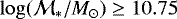 $\log (M_{*} / M_{⊙}) \geq 10.75$ $\log(\mathcal{M}_{\ast}/M_{\odot})\ge 10.75$ ) at these redshifts, a phenomenon we have verified to hold within the photometric redshift range adopted in this paper. Such galaxies would be missed if we had instead opted for a K_s -selected sample which would have resulted in a ~35% incompleteness at these stellar masses.

For analyses that involve mapping of the field either in photometric redshifts or through a combination of photometric and spectroscopic redshifts (see Sect. 3.3) we instead opt for a K_s < 24 and [3.6] < 25.4 sample. Such a cut allows us to keep a majority of high-stellar-mass galaxies in this redshift in the sample while forcing the average brightness of objects with 4 < z_phot < 5 to those similar to the spectroscopic sample such that we can reasonably apply the statistics derived in this section to this sample. Additionally, this cut yields a spectroscopic sampling rate (i.e., the number of objects targeted by all surveys versus the total number of objects) within the area covered by VUDS to a value roughly twice that of a [3.6]-limited sample (16.3 vs. 9.8%) and at ~10% for objects in the magnitude range which place them as potential members (21 < [3.6] < 25.4). This point will be especially important when we statistically combine the z_spec and z_phot samples in Sect. 3.3. It should be noted, however, that all analyses presented in this study are relatively unaffected by making cuts which are less well motivated for both portions of the analysis as long as some sort of reasonable K_s is applied tothe galaxy sample used to make various maps.

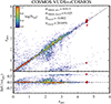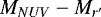
Fig. 1

Comparison of COSMOS2015 photometric redshifts ([3.6] < 25.4) versussecure spectroscopic redshifts (see Sect. 2.1) from the zCOSMOS-bright, zCOSMOS-deep, and VUDS surveys. Stars and known AGNs are included in the comparison as their identity is not generally known a priori. A scale bar indicates the density of objects in each region of the phase space. Filled red diamonds denote VUDS z_spec members of PCl J1001+0220. The σ_NMAD for the wholesample and for 4 < z < 5 along with the median offset (Δ_z = (z_phot − z_spec)∕(1 + z_spec)) and the percentage of catastrophic outliers (|z_phot − z_spec|∕(1 + z_spec) > 0.15) for the latter redshift range are shown in the main panel. Residuals are shown in the bottom panel. We note that the spectroscopic sample at z > 4 has a median [3.6] magnitude nearly one magnitude brighter (Δm = 0.85) than the z_phot sample adopted in this study meaning that these values are likely lower limits. We note also that all known catastrophic outliers at these redshifts result from the SED fitting confusing the Lyman break for the Balmer break and not the reverse, thus resulting in what is likely a pure but incomplete sample at 4 < z < 5. At z < 2 the two zCOSMOS samples dominate over VUDS providing 96.0% of all secure spectroscopic redshifts. At 2 ≤ z ≤ 3 the combined zCOSMOS samples and the VUDS sample are roughly matched in number with ~2000 spectroscopic redshifts each. At higher redshifts, z > 3 and z > 4, the VUDS sample dominates providing 83.9% and 97.3% of the secure spectroscopic redshifts, respectively.

2.2.2 Estimation of physical parameters

For galaxies with secure spectroscopic redshifts, we used three different methods to derive associated parameters. The first was to use the package LE PHARE in a method identical to the one described in Lemaux et al. (2014a). For this fitting we drew upon v2.0 of the PSF-matched photometry given in Capak et al. (2007) using all bands blueward and including Spitzer/IRAC [4.5]. The Spitzer/IRAC cryogenic bands ([5.8]/[8.0]) were excluded from the fitting due to relatively large (~1–2.5 mag) offsets seen in these bands in ~30% of all VUDS-COSMOS galaxies with respect to the best-fit model estimated without the use of these bands. We note that this issue appears limited to the Capak et al. (2007) catalog and does not apply to fitting performed with the COSMOS2015 photometry. The process of PSF-homogenizing all UV/optical/ground-based NIR images, source detection, the inclusion of the Spitzer/IRAC data, and the conversion of all magnitudes to “pseudo-total” magnitudes is described in detail in Ilbert et al. (2013). Details of this fitting including the input parameters and the effect of various assumptions made for this fitting are given in Lemaux et al. (2014a).

For some analyses, a similar fitting was performed on VUDS rest-frame near-ultraviolet (NUV) spectra in conjunction with identical photometry as in the LE PHARE analysis using GOSSIP+, a modified version of the Galaxy Observed-Simulated SED Interactive Program (GOSSIP; Franzetti et al. 2008). The details of the modifications made for GOSSIP+ as well as the fitting process as it pertains to VUDS spectra and the advantages of the fitting over traditional photometric SED fitting, particularly in regards to estimating galaxy ages, are given in Thomas et al. (2017a,b). Both methodologies, LE PHARE and GOSSIP+, use some form of a $χ_{ν}^{2}$ $\chi_{\nu}^2$ minimization in order to recover the best-fit model from which the physical parameters are estimated. In addition, both methodologies employ a nearly identical set of input parameters including Bruzual & Charlot (2003; hereafter BC03) stellar templates, models generated from exponentially declining and delayed star formation histories (SFHs), dust extinctions, and a Chabrier (2003) initial mass function (IMF). For a full listing of the parameters adopted for the fitting see Lemaux et al. (2014a) and Thomas et al. (2017a).

The final method employs the three-component SED-fitting code SED3FIT⁶ (Berta et al. 2013), which combines the emission from stars, dust heated by star formation, and a possible AGN emission component. The fiducial package of galaxy templates is taken from the Multi-wavelength Analysis of Galaxy PHYSical properties (MAGPHYS; da Cunha et al. 2008) code, which relies on an energy balance between the dust-absorbed stellar continuum and the reprocessed emission in the mid- to far-infrared. Stellar templates are taken from the BC03 library, whose output SEDs are modulated by the effects of dust attenuation and the stellar heating of dust (Charlot & Fall 2000; da Cunha et al. 2008). To this fiducial set of models, the SED3FIT code implements a set of libraries which include both an accretion disc component and a warm dust component surrounding the AGN in a smooth toroidal structure (Feltre et al. 2012; see also Fritz et al. 2006) following the method of (Berta et al. 2013). For each galaxy in our sample, we run both the SED3FIT and the MAGPHYS codes to the full COSMOS2015 photometry (Laigle et al. 2016), from FUV to 500 μm, using a common set of galaxy templates. The results of these two runs are then compared statistically (see Sect. 4.2.2) to estimate the relative contribution of various components to the global UV-IR SED (see Delvecchio et al. 2014 for details). Though the Herschel SPIRE/PACS data for the COSMOS field are relatively shallow for individual galaxies, stacked photometry of various galaxy sub-samples in this paper allows for the placing of meaningful constraints on both AGN activity and the amount of obscured star formation (see Sect. 4.2.2).

3 Discovery of a z ~ 4.57 proto-structure in the COSMOS field

In this section we describe the discovery and characterization of the highest redshift overdensity seen by VUDS. We begin by focusing exclusively on the spectroscopic overdensity, as it was in these data that the proto-structure was first detected. However, the observed characteristics and magnitude of the overdensity of VUDS proto-structures are sensitive to a variety of different aspects of the distribution of the VUDS targets spatially, in galaxy type, and in brightness. As such, we additionally classify this overdensity through the use of photometric redshifts and by combining photometric and spectroscopic redshifts in a probabilisticmanner. These methods paint a coherent picture of a highly significant overdensity assembling in the early Universe.

3.1 Overdensity as seen by spectroscopy

The initial search for overdensities, generically and non-threateningly termed “proto-structures” here and throughout this study, in the COSMOS field took an almost identical form to that described in Lemaux et al. (2014a). We briefly describe the process here. The 4895 galaxies in the COSMOS field with secure spectroscopic redshifts at z > 1.5 available to us were combined into a single catalog. In the case of duplicates, we gave preference to the redshifts with the most secure flag, or, in the case of equal flags, to VUDS redshifts. This catalog was used to generate spectral density maps of the entire COSMOS field from 1.5 ≤ z ≤ 5 in 25 Mpc slices applying the nearest-neighbor method of Gutermuth et al. (2005). These maps were searched by eye for overdensities and all those overdensities which contained seven galaxies with concordant redshifts (i.e., in the same slice) within R_proj ≤ 2 Mpc were considered as proto-structures. For each proto-structure, new maps were generated iteratively decreasing the redshift range until the overdensity was maximized. Following the generation of the final maps, luminosity-weighted and unit-weighted z_spec member centers were determined iteratively following the method of Ascaso et al. (2014) using R_proj ≤ 2 Mpc and the K_s or [3.6] bands for luminosity weighting. In total, 26 such proto-structures were found in the COSMOS field rank ordered in increasing redshift, of which one of the most significant was reported in Cucciati et al. (2014). The highest redshift of these and also one of the most significant in the entire COSMOS field, a proto-structure at z ~ 4.57 spanning 7.5 Mpc⁷ along the LOS and containing nine z_spec member galaxies (see Fig. 2), serves as the subject of this paper.

The method to determine the significance of the spectral overdensity of each of these proto-structures was identical to that of Lemaux et al. (2014a) and Smolčić et al. (2017a). Briefly, for each proto-structure, a volume equivalent to that used to define that proto-structure, that is, “filter”, was randomly placed at 1000 spatial locations securely (≥ 2 Mpc) inside the borders of the VUDS+zCOSMOS spatial coverage⁸, avoiding gaps in coverage, and at a random central redshift. Because of the rapidly varying selection and effectivenessof the zCOSMOS and VUDS surveys as a function of redshift, random central redshifts for the filters were limited to certain redshift ranges depending on the redshift of the proto-structure: 1.5 ≤ z ≤ 2, 2 ≤ z ≤ 3, 3 ≤ z ≤ 4, or 4 ≤ z ≤ 5. The angular spatial constraints listed above ensure that the density of spectroscopic targeting varies by less than a factor of two over the entirety of the area sampled, a negligible variation for this exercise. For each realization, galaxies in the spectroscopic catalog falling within the filter were counted, and the resulting distribution was fit to a Poissonian or Gaussian function, the former being used when the average number of galaxies falling within the filter was small.

This distribution and the resulting fit for the z ~ 4.57 proto-structure is shown in Fig. 3 and the resulting overdensity values given in Table 1. While there exist large formal uncertainties in the magnitude of the calculated spectral overdensity, δ_gal = 17.0 ± 6.2, where δ_gal ≡ (N_PS − μ)∕μ, the overdensity is highly significant, representing a 12σ fluctuation of the spectroscopic density field, that is, σ_PS ≡ (N_PS − μ)∕σ, where μ and σ are the mean and standard deviation, respectively, associated to the Poissonian fit performed above and N_PS is the number of spectroscopically confirmed proto-structure members. Such an overdensity is even more impressive given that the VUDS spectroscopic coverage does not continue eastward of RA ~ 150.4, meaning only ~70% of the area bounded by R_proj ≤ 2 Mpc from the number-weighted z_spec member center of the proto-structure was covered by VUDS. Given the relatively small number of confirmed z_spec members, the non-uniform VUDS coverage, the sparsity of the coeval field, and the complicated nature of the VUDS selection at these redshifts, we refrain from pushing these values further and wait for further context presented later in this section.

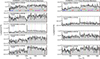Fig. 2

Individual rest-frame VUDS spectra of the nine z_spec members of the z ~ 4.57 proto-structure detected in COSMOS with secure spectroscopic redshifts (see Sect. 2.1.1 for the meaning of this phrase). The spectra were smoothed with a Gaussian filter of σ = 1.5 pixels (~1.5 Å in the rest-frame). The ID of each member galaxy along with its spectroscopic redshift, redshift quality flag, and observed i⁺ magnitude are shown on the upper left hand corner of each panel. The typical flux density uncertainty as estimated by the NMAD scatter of each spectrum over the wavelengths plotted here is 1.5 × 10⁻¹⁹ ergs s⁻¹ cm⁻² Å⁻¹. Colored dotted lines indicate important spectral features. We highlight that in many cases the Lyα emission feature is absent or an identical redshift would have been recovered even in its absence.

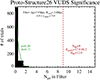Fig. 3

Spectroscopic overdensity of the z ~ 4.57 proto-structure as seen by VUDS. The black histogram shows the incidence of galaxies with secure spectroscopic redshifts falling within a “filter” of size given at the top of the plot for 1000 trial observations of the COSMOS field. For each observation the filter is placed at a random (uniformly generated) spatial location over the VUDS footprint and given a random (uniform) redshift center in the range 4 < z < 5. The filter size is chosen to be identical to that adopted for this proto-structure. The green solid line is a Poissonian fit to the histogram with best-fit parameters given to the right of the line. The number of z_spec members of the proto-structure, N_PS, is denoted by the vertical dashed line. The spectroscopic overdensity (δ_gal = (N_PS − μ)∕μ) and detection significance (σ_PC = (N_PS − μ)∕σ) of the proto-structure is listed to the right of the line.

Table 1

General properties of PCl J1001+0220.

3.2 Overdensity as seen by photometric redshifts

In Fig. 4 we show the sky location of the z_spec members of the z ~ 4.57 proto-structure plotted against the backdrop of a density map of objects with photometric redshifts (hereafter z_phot) from the COSMOS2015 catalog, consistent with that of the proto-structure, that is, z_phot ~ 4.57 ± 1.5σ_NMAD × (1 + 4.57), subject to the criteria given in Sect. 2.2 and following the nearest-neighbor method of Gutermuth et al. (2005). In order to determine the level and significance of the overdensity, if any, SExtractor (Bertin & Arnouts 1996) was run on the full COSMOS density map at the redshift of the proto-structure along with those at a variety of other redshifts. All peaks in the z_phot density map that formally exceeded 5σ detections were cataloged. Spurious peaks were identified as those that had the requisite spectroscopic coverage but which lacked a corresponding spectroscopic overdensity at ≥ 3σ_PS, where σ_PS is defined earlier in this section. As in Lemaux et al. (2014a), a Gaussian was fit to the distribution of SExtractor significances of spurious peaks⁹, with the resulting parameters used to estimate the true (spurious-corrected) significance of measured overdensities. Here, and throughout this section, we expand the projected area considered to be part of the proto-structure to 3 Mpc. While the results presented inthis section do not change appreciably if we instead consider the region which bounds the spectroscopic overdensity (R_proj ≤ 2 Mpc), we choose a larger radius here because it is better matched to the spatial size of proto-structures both in simulations (e.g., Chiang et al. 2013; Muldrew et al. 2015; Contini et al. 2016; Orsi et al. 2016) and in observations (e.g., Lemaux et al. 2014a; Dey et al. 2016; Toshikawa et al. 2014, 2016) and due to our ignorance of the true center of the proto-structure¹⁰. Furthermore, the absence of VUDS observations eastward of α_J2000 ~ 150.40° means that our spectroscopy certainly does not probe the full extent of the proto-structure. Thus, we take here an inclusive approach. There appears both a significant raw (20.7) and spurious-corrected (4.7) overdensity in the region centered on the z ~ 4.57 VUDS-COSMOS proto-structure. It is important to note this overdensity is not necessarily redundant evidence of an overdensity of galaxies as VUDS certainly does not target nor detect most L^* galaxies at this redshift and the number of galaxies required to create such an overdensity, assuming the catastrophic outlier rate given in Sect. 2.2, considerably exceeds the number of z_spec members.

However, despite the use of arguably the best z_phot measurements made to date, such measurements are moderately prone to fail catastrophically (see Fig. 1) and, even if correct, to adopt the approach of a binary z_phot membership criteria given the large extent in redshift space required by the z_phot precision (Δ_z = 0.42) is perhaps overly coarse. While we will employ a more complex statistical combination of photometric and spectroscopic redshifts in the following section to quantify the overdensity, we attempt one other method here to determine the genuineness of the z_phot overdensity. The full probability distribution functions (PDFs) generated by Le Phare for each z_phot member were re-constructed using the effective uncertainties in the z_phot values and, when necessary, those of secondary peaks in the z_phot PDF which exceeded 5% of the overall probability density. These re-constructed PDFs were combined into a single composite PDF shown in the bottom right panel of Fig. 4 as a green filled histogram. Simultaneously, the same process was performed for all objects in the COSMOS2015 catalog, subject to the criteria set in Sect. 2.2, with z_phot = 4.57 ± 1.5σ_NMAD × (1 + 4.57) but outside of the projected spatial cut (coeval z_phot field). The combined distribution of these objects is shown in the bottom right panel of Fig. 4 as the blue hashed histogram. The combined PDF of the coeval z_phot field sample appears roughly flat from 4.35 ≤ z_phot ≤ 4.67, a redshift range which contains ~85% of relatively peaked z_phot measurements ( $σ_{z_{p h o t}} < 0.3$ $\sigma_{z_{phot}} < 0.3$ ) in this sample and ~80% of all objects in the coeval z_phot field. In stark contrast, the combined PDF of z_phot members has its largest peak within the spectroscopic redshift bounds of the proto-structure. Indeed, by this analysis z_phot members are nearly twice as likely as coeval z_phot field objects to be within the true redshift bounds of the proto-structure, 16% versus 9%, respectively. Such a result strongly suggests that the overdensity observed amongst the z_phot objects at the location of the proto-structure is genuine.

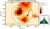Fig. 4

Sky plot of the highest redshift proto-structure detected from VUDS spectroscopy (PCl J1001+0220). Plotted in the background is the smoothed (2.5 pixels FWHM) density map for all objects with z_phot =4.57 ± 1.5σ_NMAD × (1 + 4.57) with the scale in gal/Mpc indicated by the color bar to the right. Additionally, all galaxies from VUDS+zCOSMOS with z > 2 with secure spectroscopic redshifts are plotted in the background as small gray dots. The density of these points drops precipitously to the east of the proto-cluster center owing to a lack of VUDS coverage of this area. Galaxies with secure and less secure (see Sect. 2.1) spectroscopic redshifts consistent with the redshift range of the proto-structure (4.53 <z < 4.60) are represented by filled circumscribed circles and Xs, respectively. Blue and red symbols differentiate galaxies at the redshift of the proto-structure by their rest-frame $M_{N U V} - M_{r^{'}}$ $M_{NUV}-M_{r^{\prime}}$ colors (younger and older than 200 Myr, respectively, see Sect. 4.2.1) and are logarithmically scaled (log₄) by their stellar mass. The dashed gray and black circles (R_proj = 2 and 3 Mpc from the proto-structure center, respectively) set the boundaries for z_spec and z_phot members, respectively. Plotted on the bottom right is a histogram of all secure spectroscopic redshifts within R_proj < 2 Mpc ofthe proto-structure center. Plotted in the background is the combined PDF of z_phot members (green filled) and non-members (dark blue hatched) with redshifts consistent with the redshift of the proto-structure.

3.3 Overdensity as measured by Monte-Carlo voronoi tessellation

We have now determined unequivocally that an overdensity is observed in both spectroscopic and photometric redshifts in the area encompassing PCl J1001+0220¹¹. However, both of these methods have their limitations. In the case of the former, though accurate high-precision measurements are made, only ~10% of potential (z_phot) members were targeted for spectroscopy, with the targeting having a complex dependence on galaxy type, the level of current star formation, and intervening structure. For example, because VUDS generally targets objects with 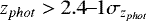$z_{p h o t} > 2.4 - 1 σ_{z_{p h o t}}$ $z_{phot}>2.4\!\!-\!\!1\sigma_{z_{phot}}$ , a true projected dearth of galaxies along the LOS at lower (z ~ 2–4) redshifts means a higher chance of targeting higher-redshift galaxies and, thus, finding a proto-structure like PCl J1001+0220. Conversely, while the z_phot methods presented in the previous section allow for an essentially stellar-mass-limited sample largely independent of galaxy type, though subject to the caveats discussed in Sect. 2.2.1, estimates are model dependent and have moderate accuracy and coarse precision at these redshifts. A method which combines both samples statistically can, in principle, help to mitigate the shortcomings of each sample.

To this end, we introduce here a modified version of the Voronoi tessellation measure of the density field employed by a variety of other studies in the COSMOS field which rely almost exclusively on photometric redshifts (e.g., Scoville et al. 2013; Darvish et al. 2015; Smolčić et al. 2017a). The method that we employ here most resembles the “weighted Voronoi tessellation estimator” introduced in Darvish et al. (2015). In that study it was found that using this method to recover the underlying density field matched or exceeded the accuracy and precision of all other methods of density estimation. The one metric with comparable performance to the Voronoi approach, weighted adaptive kernel estimation, is sensitive to both the form and size of the kernel and, generally, employs a spatially symmetric kernel (along the transverse dimensions) which is not ideal for the complex transverse shape of proto-structures.

Our version of this method is as follows. Beginning at z = 2 and reaching up to z = 7 in 7.5 Mpc steps (i.e., half the size of a slice), a suite of ten Monte Carlo realizations of the magnitude-cut nearest-neighbor-matched master spectroscopic and COSMOS2015 z_phot catalogs were generated for each step. This number of realizations was a compromise between computational intensity and stability of the resultant density estimates. For each Monte Carlo realization, first we selected the spectroscopic sub-sample by drawing from a uniform distribution ranging from 0 to 100 and retaining those z_spec measurements where the drawn number exceeded 75, 95, and 99.5 for those measurements with flags X2∕X9, X3, and X4, respectively. These thresholds follow the fiducial reliability estimates of the VUDS/zCOSMOS flagging system (see e.g., Le Fèvre et al. 2015). Such a method allowed for the incorporation of the statistical reliability of these measurements. If the pre-determined threshold was not exceeded, z_spec would be retained for that realization, otherwise it was replaced with the z_phot information. For each object where the z_phot information was used or was the only information available, the original z_phot for that object was perturbed by sampling from an asymmetric Gaussian distribution with σ values that correspond to the lower and upper effective 1σ z_phot uncertainties.

Voronoi tessellation was then performed on each realization at each redshift step on objects with redshifts falling within ±7.5 of the central redshift of each bin, that is, a bin width of Δχ = 15 Mpc or Δ_z ~ 0.03–0.3 from z ~ 2–7. The 7.5 Mpc steps between slices along with the slice thickness ensure overlap between successive slices such that we do not miss overdensities by randomly choosing unlucky redshift bounds. For each realization of each slice, a grid of 75 × 75 kpc was created to sample the underlying local density distribution. The local density at each grid value for each realization and slice was set equal to the inverse of the Voronoi cell area (multiplied by $D_{A}^{2}$ $D_{A}^2$ ) of the cell that encloses the central point of that grid. Final local densities, Σ_{V MC}, for each grid point in each redshift slice are then computed by median combining the values of ten realizations of the Voronoi maps. The local overdensity value for each grid point is then computed as $\log (1 + δ_{g a l}) \equiv \log (1 + (Σ_{V M C} - {\tilde{Σ}}_{V M C}) / {\tilde{Σ}}_{V M C})$ $\log(1+\delta_{gal}) \equiv \log(1+ (\mathrm{\Sigma}_{VMC}-\tilde{\mathrm{\Sigma}}_{VMC})/\tilde{\mathrm{\Sigma}}_{VMC})$ , where ${\tilde{Σ}}_{V M C}$ $\tilde{\mathrm{\Sigma}}_{VMC}$ is the median Σ_{V MC} for all grid points over which the map was defined, that is, excluding a border region of ~1′ in width to mitigate edge effects. In preliminary tests of the method employed for our study we observed realistic mock catalogs of proto-clusters and proto-groups with a combination of deep spectroscopy and photometric redshifts with COSMOS2015-level precision and accuracy. It was found that the overdensity field estimated by our method after an identical magnitude cut resembling that applied to our true sample used for the mapping (i.e., Ks < 24) falls within <30% of the true (i.e., real space) overdensity field essentially independent of the value of overdensity, the redshift, or the spectroscopic completeness, as long as the latter is in excess of ~10%, a value similar to that of this study (see Sect. 2.2.1). While reconstruction is still possible when the spectroscopic completeness is lower, the relative accuracy drops immensely, with the reconstructed values deviating by up to ~200% away from the true value when the sampling drops to ~3%. The results of these tests will be presented in depth in a future work.

Once a proto-structure was identified, as in the case of PCl J1001+0220, zoom Monte Carlo Voronoi mappings were made by iteratively shifting the redshift bounds to find the values most appropriate to that particular proto-structure. For PCl J1001+0220, these values were found to be identical to the redshift range of the z_spec members, 4.53 ≤ z ≤ 4.60. Once the redshift bin was chosen, 500 Monte Carlo realizations were performed for that redshift slice, with the resultant final density and overdensity maps generated using an identical method to the mapping described earlier. The latter of these two maps for PCl J1001+0220 is shown in Fig. 5. Following the generation of these maps for PCl J1001+0220, SExtractor was run on the overdensity maps for the purpose of quantifying both the significance and the extent of the proto-structure using log (1 + δ_gal) > 0.5 as a detection threshold. The resulting detection of PCl J1001+0220 extends over an area of 7.58 Mpc² and has an average log (⟨1 + δ_gal⟩) = 0.63 ± 0.03. The uncertainty is determined from the dispersion around both the average density contained within the region defining PCl J1001+0220 and the median density of the full slice as measured in all 500 realizations. We adopt this overdensity value and its associated uncertainty as being the most reliable estimate of the galaxy overdensity of PCl J1001+0220. Because this value exceeds the value for equivalent galaxy populations of nearly all simulated proto-clusters at these redshifts when viewed over an equivalent volume, (~21 comoving Mpc³, see Table 4 of Chiang et al. 2013), here and for the rest of the paper we abandon the term proto-structure when referring to the PCl J1001+0220 proto-cluster. It is also perhaps revelant to note that at this galaxy overdensity, assuming the galaxy bias value given in Sect. 4.1 and pressureless spherical collapse, the entire proto-cluster as defined over the volume above collapses well before z ~ 0. Each overdensity value and central coordinate computed in this section, as well as a variety of other information on the PCl J1001+0220 proto-cluster, is given in Table 1.

Fig. 5

Sky plot of the Voronoi Monte-Carlo overdensity map encompassing a large fraction of the VUDS coverage in the COSMOS field. The redshift bound over which the Voronoi tessellation is calculated is set to 4.53 < z < 4.60. Both spectroscopic and photometric redshifts are treated statistically following the prescription in Sect. 3.3 and used generate 500 realizations of the overdensity map in the field. These 500 maps are then median combined and smoothed with a Gaussian of FWHM = 4.5 pixel to create the plotted map. A color bar indicates the magnitude of the overdensity in each 75 × 75 kpc² pixel. The dashed line indicates the extent of our z_spec member cut (R_proj = 2 Mpc). Small black dots denote galaxies with secure spectroscopic redshifts at z > 3 from VUDS and filled circumscribed blue diamonds denote those within the range of PCl J1001+0220. The PCl J1001+0220 proto-cluster exhibits coherent overdensity (log (1 + δ_gal) > 0.5) over an area of 7.58 Mpc².

4 Properties of the PCl J1001+0220 proto-cluster

With the identity of the PCl J1001+0220 proto-cluster now firmly established, in this section we attempt to contextualize this proto-cluster and to make a cursory exploration of the properties of its member galaxies using all the information at our disposal.

4.1 Weighing the PCl J10001+0220 proto-cluster

At lower redshifts (z ≤ 1.5), a clear correlation exists between the total mass of a structure and the evolutionary state of its constituent galaxy population (e.g., Moran et al. 2007; Poggianti et al. 2008, 2009; Hansen et al. 2009; Lubin et al. 2009; Lemaux et al. 2012; van der Burg et al. 2014; Balogh et al. 2016). While dispersion in this correlation exists, and while the evolutionary state of a galaxy population clearly has acomplex relationship with other factors either causally or circumstantially connected with global environment, such as local (over)density, stellar mass, and global dynamics, estimating the total mass for a structure is a necessary step in predicting the fate of that structure and its constituent galaxy population. At such redshifts reasonably precise estimates are at least achievable with current technology through strong or weak lensing, X-ray observations, and dynamics measurements from exhaustive spectroscopic campaigns. While widely employed, these estimates necessarily have (relatively) large systematic uncertainties originating from the large number of assumptionsrequired to even attempt a measurement with these data. Furthermore, at the highest redshifts in this redshift range z ~ 1.5, only the most exquisite data sets can be reasonably employed to estimate total masses, as sparser sampling, differential bias in sampling, and/or lower signal-to-noise ratio (S/N) data makes it impossible to begin to probe the validity of these assumptions.

At higher redshift, the situation becomes much more dire. Precision estimates of total masses through lensing and X-ray measurements become nearly impossible. Quiescent galaxies, whose global dynamics should, generally, better trace the underlying potential than other galaxy populations, become sparser and more difficult to detect spectroscopically, a requisite condition of any dynamics analysis. Furthermore, assumptions which generally come close to being valid for massive overdensities at lower redshift, for example, virialization, and hydrostatic equilibrium, almost certainly do not hold at these redshifts. Further, proto-clusters appear in simulations to have extremely complex morphologies, and overdensity estimates, estimates which are subsequently translated into total masses, appear to be strongly dependent on viewing angle (Shattow et al. 2013). Given these difficulties, here we attempt a variety of different methods (as was done in Lemaux et al. 2014a) to estimate the total mass of PCl J1001+0220. Because each of these methods requires a different set of assumptions, the above uncertainties are, to the best of our ability, minimized, allowing for at least the potential to triangulate the requisiteaccuracy to properly contextualize the PCl J1001+0220 proto-cluster when the estimates are averaged. Note that, for all proto-cluster estimates, the term “total mass” is meant to refer to the composite mass of all halos which comprise the proto-cluster (or the eventual cluster) rather than the mass of the most massive halo in the (proto-)cluster. As pointed out in, for example, Muldrew et al. (2015), the most massive halo for all high-redshift proto-clusters likely contains a small fraction of proto-cluster galaxies and a small fraction of the overall mass (≲10% for both cases).

Under the assumption of virialization and isotropic motion, the LOS dynamics of satellite galaxies provide a readily available proxy for the total mass. Though the redshift of Cl1001+0220 makes it extremely unlikely that the observed members have reached a near-virialized state, and though the time at which a system is observed in its dynamical history dictates whether the dispersion of the observed LOS differential velocities is an overestimate or underestimate relative to it virial equivalent (see e.g., Cucciati et al. 2014), neither of these possibilities precludes the possibility that such a measurement could provide useful information. Indeed, the member galaxies in both simulations of cluster progenitors (Cucciati et al. 2014)and in large compilations of observed proto-clusters (Franck & McGaugh 2016b) exhibit velocity dispersions, and, by consequence, dynamical masses, which correlate, weakly but significantly, with masses derived through independent estimates. In Fig. 6 we plot the differential LOS velocity dispersion of all nine members of Cl1001+0220 along with the biweight fit to distribution. The estimated LOS velocity dispersion of 1038 ± 178 km s⁻¹ correspondsto a virial mass of: $\log {(M_{v i r} / M_{⊙})}_{z ~ 4.57, d y n} = 14.39 \pm 0.22.$ $\begin{equation*} \log(\mathcal{M}_{vir}/\mathcal{M}_{\odot})_{z\sim4.57, dyn} = 14.39\pm0.22.\end{equation*}$ (1)

While this is an immense total mass at this redshift, it is possible that galaxy dynamics provide a gross overestimate due the effects described above. The level by which this dynamical mass might exceed the true total mass can be crudely estimated by applying the average offset between dynamical masses and masses estimated by matter overdensities, in those cases where both were definitely measured, for the large ensemble of proto-clusters compiled by Franck & McGaugh (2016b). Though it is not clear that overdensity masses necessarily more accurately reflect true total masses, the methods used in that study differ from those used here, and there exists a large scatter in this distribution (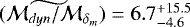 $\tilde{(M_{d y n} / M_{δ_{m}}}) = {6.7}_{- 4.6}^{+ 15.5}$ $\widetilde{(\mathcal{M}_{dyn}/\mathcal{M}_{\delta_{m}}}) = 6.7^{+15.5}_{-4.6}$ , median and effective 1σ scatter); such a correction can perhaps provide a reasonable range of values in which the true total mass resides. Applying this median correction and propagating its uncertainties into the resultant corrected value yields $\log {(M_{v i r} / M_{⊙})}_{z ~ 4.57, d y n, c o r r} = {13.6}_{- 1.0}^{+ 0.4}$ $\log(\mathcal{M}_{vir}/\mathcal{M}_{\odot})_{z\sim4.57, dyn, corr}=13.6^{+0.4}_{-1.0}$ .

A different approach is to count the amount of baryonic material within the proto-cluster bounds associated with the member galaxies and attempt to relate that back to the overall mass of the structure, an approach which has been employed successfully at low redshift when the galactic baryonic content of cluster member galaxies is dominated by stars (Andreon 2012). The approach we take here is similar to that of Lemaux et al. (2014a). Briefly, the total amount of stellar matter of the z_spec members is counted and a completeness correction is made to this value for galaxies at stellar masses $\log (M_{*} / M_{⊙}) \geq 9.5$ $\log(\mathcal{M}_{\ast}/M_{\odot})\ge 9.5$ (see Sect. 4.2.1 for the reasoning behind this cut) based on the number of z_phot members and non-members without secure spectral redshifts within the bounds of the proto-cluster and the likelihood of their being true members. An additional correction is made to correct for galaxies in the stellar mass range $8.0 < \log (M_{*} / M_{⊙}) < 9.5$ $8.0 < \log(\mathcal{M}_{\ast}/M_{\odot})< 9.5$ by integrating the stellar mass function of Davidzon et al. (2017) appropriate for this redshift. Here we additionally make the assumption that stellar mass comprises 50% of the baryonic content of galaxies by mass at these redshifts, a value broadly consistent with the few measurements made at or near these redshifts (e.g., Tacconi et al. 2010; Capak et al. 2011b; Schinnerer et al. 2016; Scoville et al. 2016). We assume for the purposes of this calculation that the proto-cluster is a closed system, with all gas being converted to stars by z = 0 and that the completeness-corrected galaxy population which lies within R_proj ≤ 3 Mpc at z ~ 4.57 comprises the entirety of the galaxy population which will eventually be contained within the cluster virial radius at z = 0. The latter assumption is broadly consistent with simulations (Muldrew et al. 2015) to ~10% accuracy, a factor which we account for in the calculation below. Any total to stellar mass conversion then provides a z = 0 total mass, which we de-evolve to z ~ 4.57 using the correction factors of Muldrew et al. (2015) appropriate for z ~ 4.57 (0.20 ± 0.03), a correctionwhich is appropriate for descendents of all masses. Into this formalism we input the resulting completeness-corrected baryonic content of $\log (Σ M_{*} / M_{⊙}) = {12.39}_{- 0.07}^{+ 0.05}$ $\log(\mathrm{\Sigma}\mathcal{M}_{\ast}/M_{\odot})=12.39^{+0.05}_{-0.07}$ to the r₂₀₀ stellar mass to M₅₀₀ total mass relation of Andreon (2012) and scale the resulting M₅₀₀ to the virial radius (R_vir = 0.33 Mpc) using the methods presented in Lemaux et al. (2014a) giving: $\log {(M / M_{⊙})}_{z = 4.57, Σ M_{*, c o r r}} = {13.31}_{- 0.27}^{+ 0.23} .$ $\begin{equation*} \log(\mathcal{M}/\mathcal{M}_{\odot})_{z=4.57, \, \mathrm{\Sigma}\mathcal{M}_{\ast, corr}} = 13.31^{+0.23}_{-0.27}.\end{equation*}$ (2)

We note that this estimate, within the context of this formalism, is almost certainly a lower limit to the total mass of the proto-cluster given that there exists diffuse gas at z ~ 4.57, which we do not account for here, of which some fraction will undoubtedly be accreted and used to create stars by z = 0. This lack of precision may be mitigated somewhat by the fact that we also do not account for the loss of stellar and gaseous material in member galaxies due to, for example, tidal or ram pressure stripping or by merging activity as the proto-cluster evolves. Despite all the uncertainties related to this calculation, if the completeness-corrected baryonic content of the proto-cluster is instead used in conjunction with the universal dark-to-baryonic fraction of 6.42 ± 0.19 (Planck Collaboration XIII 2016) to estimate the total mass, the result, $\log {(M / M_{⊙})}_{z = 4.57, Σ M_{*, c o r r}}$ $\log(\mathcal{M}/\mathcal{M}_{\odot})_{z=4.57, \, \mathrm{\Sigma}\mathcal{M}_{\ast, corr}}$ =13.20 $_{- 0.07}^{+ 0.05}$ $^{+0.05}_{-0.07}$ , is nearly identical to the above calculations. Nevertheless, all three of these estimates place the descendant total mass of PCl J1001+0220 at or above M_h,z=0 = 10¹⁴ once evolved to z = 0 following the formalism of McBride et al. (2009) and Fakhouri et al. (2010) (see Lemaux et al. 2014a for its implementation in this context) or Muldrew et al. (2015). Again, however, these methods relied on a number of assumptions which, while perhaps applicable generally, may or may not be valid for this particular proto-cluster.

The final method we employ here relies on the galaxy overdensity as measured from the Voronoi Monte Carlo technique in an attempt to relate this overdensity to the present day total mass through large-scale simulations (Chiang et al. 2013). As such, though this method is model dependent, neither the galaxy velocities, the lack of complete spectroscopic sampling, nor the bulk properties of the galaxies themselves should affect this estimation. This estimation follows that of Lemaux et al. (2014a) nearly identically and, as such, we do not repeat the formalism here. The one major exception for this study is the replacement of the spectroscopic overdensity, used previously, with the Voronoi Monte Carlo overdensity making the estimate much less uncertain and much less dependent on sampling effects. As we have also changed the volume used to calculate this overdensity, a volume which is now set by the SExtractor detection (segmentation) map (see Sect. 3.3) and the adopted redshift range of the proto-cluster, a correction is made following Chiang et al. (2013) to account for additional mass outside of the volume used (e.g., similar to an aperture correction, see also Muldrew et al. 2015). The correction factor is taken to be 1/0.8, appropriate for the segmentation-estimated proto-cluster volume which has an effective radius (R_e) of 10.9 comoving Mpc (see Chiang et al. 2013 for more details). We have also adopted here a bias parameter of b = 3.60, a reasonable estimate for the redshift and galaxy sample used here (Chiang et al. 2013; Durkalec et al. 2018). The final descendant mass of PCl J1001+0220 is then estimated to be: $\log {(M_{h} / M_{⊙})}_{z = 0, (1 + δ_{g a l})} = 14.48 \pm 0.03,$ $\begin{equation*} \log(\mathcal{M}_{h}/\mathcal{M}_{\odot})_{z=0, (1+\delta_{gal})} = 14.48\pm0.03,\end{equation*}$ (3)

a descendant mass intermediate to those estimated by the other two methods. It is important to note, though, that this descendant mass is not cause for ambiguity in the overall nature of PCl J1001+0220; the galaxy overdensity value used here along with the area over which that overdensity was measured still places PCl J1001+0220 as a proto-cluster at >80% confidence (Chiang et al. 2013). The $M_{h, z = 0, (1 + δ_{g a l})}$ $\mathcal{M}_{h, z=0, (1+\delta_{gal})}$ estimated above is broadly similar to the value derived from the formalism of Orsi et al. (2016), a study which employs vastly different models and assumptions. While it is necessary to assume for the latter that the proto-cluster contains a quasar or radio galaxy which has yet to be observed and that, further, the density of faint Lyα emitters scales directly with the density of ~ L^* galaxies at these redshifts, the concordance in $M_{h, z = 0, (1 + δ_{g a l})}$ $\mathcal{M}_{h, z=0, (1+\delta_{gal})}$ estimates between these two methods is encouraging. Regardless of the method chosen, the large descendant mass estimated for PCl J1001+0220 requires, under the formalism of models predicting typical mass growth (Fakhouri et al. 2010; Muldrew et al. 2015), that considerable amount of mass assembles ( $\log (M_{h} / M_{⊙}) \ga 12$ $\log(\mathcal{M}_{h}/M_{\odot})\ga12$ ) before the end of the epoch of reionization (i.e., z ~ 6). As such, the progenitors of systems like PCl J1001+0220 can be, under certain circumstances, useful in differentiating between different models of reionization (see D’Aloisio et al. 2015; Castellano et al. 2016; Davies & Furlanetto 2016 and references therein). Because none of our results are dependent on the exact total mass of PCl J1001+0220 either at z ~ 4.57 or at z = 0, we satisfy ourselves with the understanding that PCl J1001+0220 is a massive proto-cluster that will evolve into a cluster at low redshift with an overarching mass somewhere in between that of the Fornax and Coma clusters (Kent & Gunn 1982; Colless & Dunn 1996; Nasonova et al. 2011).

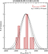Fig. 6

Differential velocity distribution of the z_spec members of PCl J1001+0220. The median redshift of z_spec member galaxies is shown in the top right corner of the plot. Also shown in the top right corner is the value of the best-fit line of sight (LOS) velocity dispersion (σ_v, see Sect. 3 for details). The resulting Gaussian function generated by the best-fit σ_v is overplotted on the differential velocity histogram (solid black line) along with those functions generated from $σ_{v} \pm σ_{σ_{v}}$ $\sigma_{v}\pm\sigma_{\sigma_v}$ .

4.2 An investigation of environmentally driven evolution at z ~ 4.57

From the previous sections we have determined that the member galaxies of PCl J1001+0220 reside in a globally dense (i.e., proto-cluster) environment that exhibits a large-scale coherent elevated local density. Though strong correlations between galaxy properties and both local and global environment are observed at lower redshifts (z≲2, e.g., Goto et al. 2003; Postman et al. 2005; Cooper et al. 2007; Muzzin et al. 2012; Lemaux et al. 2012; Cooke et al. 2016; Davidzon et al. 2016; Lemaux et al. 2017), such correlations, if they exist, are far from established at higher redshifts. In this section we use every method at our disposal to determine if the onset of environmental effects have imprinted themselves onto the galaxy population of PCl J1001+0220 just 1.3 Gyr after the Big Bang.

4.2.1 Luminosity, color, stellar mass, and age properties

We begin by comparing quantities derived from our various SED fitting techniques for PCl J1001+0220 member and coeval field samples defined in a variety of ways. We choose to use a variety of techniques as well as a variety of sample definitions to mitigate our ignorance of the true center of the proto-cluster, our ignorance of both the redshift and transverse extent of the member population, the lack of VUDS spectroscopic targeting in much of the eastern quadrants of the proto-cluster, and the various systematic and random uncertainties in SED fitting methods, uncertainties which are almost certainly exacerbated at these redshifts. Throughout these comparisons, the member and coeval field samples will always, by design, have the same median redshift and will be consistently cut at the various limits imposed. In Appendix B we describe in detail the definitions for the various samples used in the analysis in the remainder of this paper as well as the statistical approaches used to compare these samples.

In the left panel of Fig. 7 we plot the rest-frame $M_{N U V} - M_{r^{+}}$ $M_{NUV}-M_{r^+}$ versus $M_{r^{+}}$ $M_{r^+}$ color-magnitude diagram (CMD) of the z_spec PCl J1001+0220 proto-cluster members against the backdrop of the coeval field for all galaxies with $\log (M_{*} / M_{⊙}) \geq 9.7$ $\log(\mathcal{M}_{\ast}/M_{\odot})\ge 9.7$ . The area of this phase space where VUDS begins to become unrepresentative of the underlying photometric sample is shaded out. These bands are chosen as they discriminate galaxies of different ages in the absence of a copious dust content (Arnouts et al. 2013; Moutard et al. 2016), which, as we show below, is likely minimal, on average, in both samples. Additionally, by selecting these colors, we guarantee that each galaxy in the selected sample was significantly detected in at least one observed-frame band that has reasonably similar wavelength coverage at z ~ 4.57 to each of these rest-frame bands¹². Such a guarantee minimizes k-correction necessary to calculate the rest-frame magnitudes and thus the model dependence of these magnitudes. The overplotted tracks show BC03 model-derived colors, absolute magnitudes, and stellar masses as generated by EZGAL¹³. These models, which employ a variety of different SFHs, stellar-phase metallicities, and epochs of the most recent major star formation event, were designed to match the brightness of a z ~ 0.6 L^* cluster galaxy (De Propris et al. 2013) after passively evolving for ~7 Gyr (i.e., the difference in lookback time between z ~ 4.57 and z ~ 0.6).

Despite having both what is, by far, the reddest galaxy in VUDS at these redshifts and several other redder galaxies fall within the ~1% of the volume of the VUDS-COSMOS field at these redshifts spanned by the proto-cluster, a statistical difference relative to the field is not observed. Neither a KS test nor a comparison of the average $M_{N U V} - M_{r^{+}}$ $M_{NUV}-M_{r^{+}}$ colors of the member and coeval field samples ( $\tilde{M_{N U V} - M_{r^{+}}} = 1.15 \pm 0.15$ $\widetilde{M_{NUV}-M_{r^{+}}}=1.15\pm0.15$ vs. 1.11 ± 0.08, respectively) reveals any significant difference between the two populations. The proto-cluster also contains the brightest as well as three of the top ten brightest rest-frame optical galaxies in VUDS at these redshifts, and though, again, a KS test fails to find a significant difference (~1σ), a comparison of the average $M_{r^{+}}$ $M_{r^{+}}$ magnitudes yields marginally significant hints of a difference between the two populations ( $\tilde{M_{r^{+}}} = - 23.30 \pm 0.20$ $\widetilde{M_{r^{+}}}=-23.30 \pm 0.20$ vs. − 22.87 ± 0.08, respectively). In the right panel of Fig. 7 we plot a rest-frame color-stellar mass diagram (CSMD) of the same two samples. The trend in magnitude hinted in the CMD appears to be manifest in the CSMD more significantly. Two of the four most (stellar) massive galaxies in the entire spectroscopic sample at these redshifts, both of which appear to contain a suggestively old luminosity-weighted stellar population (>200 Myr), lie within the bounds on the proto-cluster. Galaxies in this region of the phase space, $\log (M_{*} / M_{⊙}) > 10.6$ $\log(\mathcal{M}_{\ast}/M_{\odot})>10.6$ , $M_{N U V} - M_{r^{+}} > 1.5$ $M_{NUV}-M_{r^{+}}>1.5$ , have, broadly, already formed the requisite stellar material to passively evolve to lower redshift L^* red-sequence galaxies. The presence of these two galaxies alone hint that this population is relatively more abundant in the proto-cluster than in the field (2/9 vs. 2/54), an inference which does not depend especially on the specific limits chosen here and one which we attempt to expand on below when comparing z_phot members. A KS test (2.5σ) and a comparison of the average stellar masses of the member and coeval field galaxies ( $\log (\tilde{M_{*}} / M_{⊙}) = 10.34 \pm 0.08$ $\log(\widetilde{\mathcal{M}_{\ast}}/M_{\odot})=10.34\pm0.08$ and 10.09 ± 0.03, respectively) additionally both suggest that the average member galaxy has built up a more massive stellar content relative to other galaxies in the field. We note that these conclusions and those below comparing stellar mass distributions of z_phot members and non-members are unchanged if we instead compare inverse error-weighted means.

The above comparisons were made with only the spectral members and exclusively using one of the SED fitting techniques we have at our disposal. Though we have gone to extreme lengths to ensure that the VUDS sample is largely representative of the underlying population of galaxies at these redshifts within the selected color and stellar mass range and that the SED method chosen is reliable at these redshifts, we now attempt two different reformulations of the analysis in order to understand if the trends hinted at in the above analysis are robust to changing the analysis framework. We begin by considering the z_phot member sample and contrasting it with the z_phot coeval field sample (see Sect. 3.2 for the definition of each sample). While it is not necessary that differences seen in the previous analysis persist in significance or gain traction, as the photometric redshifts blur the lines between the proto-cluster and the coeval field considerably, any agreement would lend veracity to the claims made with the relatively small spectroscopic sample. In the left panel of Fig. 8 we compare the stellar mass distribution of all z_phot members and the coeval field sample to the stellar mass limit of $\log (M_{*} / M_{⊙}) > 9.5$ $\log(\mathcal{M}_{\ast}/M_{\odot})>9.5$ . A comparison of the median stellar masses ( $\log (\tilde{M_{*}} / M_{⊙}) ~ 9.9$ $\log(\widetilde{\mathcal{M}_{\ast}}/M_{\odot})\sim9.9$ in both cases) and a KS test return no significant difference between the two samples. If, however, we instead restrict the sample to those galaxies with $M_{N U V} - M_{r^{+}} \geq 1.5$ $M_{NUV}-M_{r^{+}}\ge1.5$ , which, according to the models overplotted in Fig. 7 have ages that are ≥200 Myr, the two populations begin to differentiate themselves. Both a comparison of the average stellar mass of the two populations and a KS test return differences at >3σ, with the redder galaxies in the proto-cluster appearing at much higher stellar masses than their coeval field counterparts; $\log (\tilde{M_{*}} / M_{⊙}) = 10.61 \pm 0.06$ $\log(\widetilde{\mathcal{M}_{\ast}}/M_{\odot})=10.61\pm0.06$ versus 10.22 ± 0.02, respectively.The relative overdensity within the proto-cluster bounds of possible progenitors to low-redshift cluster L^* galaxies hinted at in the spectral member sample is also hinted at here ( $f_{r e d, L^{*}}$ $f_{red, L^{\ast}}$ =14.6±4.2 vs. 8.2±0.7%).

As a final check on these results, we shift back to considering only the spectral sample and plot in Fig. 9 the stellar masses and formation age (age_f¹⁴ hereafter) of the member and coeval field galaxies derived following the combination spectral and photometricfitting methodology of Thomas et al. (2017b). For all fits we required a “fitting flag” of ≥2 corresponding to good or excellent fits to both the spectroscopy and photometry for each galaxy. The fitting method used to derive these parameters is considerablydifferent in scope, in the range of models used, and in input than those used in any of the previous analysis presented in this section, and has been found to accurately and precisely recover the ages of simulated galaxies using VUDS-like observationsunder the assumption that the SFHs of galaxies at these redshifts can be approximated well by the range of SFHs assumed in our fitting process (see Thomas et al. 2017b for more details). Again, a difference between the two populations is observed in the stellar mass distribution in that galaxies in the proto-cluster are, on average, more massive in their stellar content ( $\tilde{\log (M_{*} / M_{⊙})} = 10.51 \pm 0.07$ $\widetilde{\log(\mathcal{M}_{\ast}/M_{\odot})}=10.51\pm0.07$ vs. 10.05 ± 0.04). Here, however, we additionally see a clear difference between the two populations in their age in that galaxies in the proto-cluster appear older ( ${\tilde{age}}_{f} = 904 \pm 63$ $\widetilde{\textrm{age}}_{f}=904\pm63$ vs. 640 ± 41 Myr) than the coeval field population. These differences are also significant at the ≥2.5σ level for both parameters when using a KS test. The observed difference in the ages of the two sub-samples is in apparent contrast to the lack of significant difference between the two spectroscopic populations seen in the rest-frame colors. However, the methods used by Thomas et al. (2017b) are considerably more advanced than that used to generate the models overplotted in Fig. 7, with the former method employing a vastly larger array of SFHs, treatment for the effects of extinction, and the virtue of numerous tests performed on its precision and accuracy. A similar comparison of z_phot members and coeval field galaxies could not be performed as the method of Thomas et al. (2017b) requires spectroscopy. Regardless, the common element of all three analyses presented here appears to be, at varying degrees of significance, a fractional excess within the proto-cluster of older, and, in some analyses, redder, galaxies which appear more massive in their stellar content. The large differences in stellar masses compared to what are relatively small differences in ages (or colors) necessarily implies that, on average, a proto-cluster galaxy must have a more violent SFH than their field counterparts, with stellar mass being built up more rapidly after their formation. As we will show in the following section, the two populations have indistinguishable instantaneous SFRs (integrated over ~100 Myr), which, in conjunction with the results presented in this section, further implies that there is something necessarily different about the SFHs of the two populations.

The slope, β, of the continuum flux density in the rest-frame ultraviolet (f_λ ∝ λ^β) has been shown, for a given IMF and a given dust geometry and law, to correlate well with the level of dust in a galaxy (e.g., Meurer et al. 1999; Reddy et al. 2010; Álvarez-Márquez et al. 2016). As the analysis throughout this section relied heavily on the difference in the colors and various ages of member and coeval field samples, and as the precision and meaning of such parameters can be heavily influenced by the presence of dust, an independent measure of the dust content is important to gain context on the reliability of these results and their interpretation. In Fig. 10 we plot the distribution of β slopes measured for the member and coeval field samples. While, in principle such measurements could be made directly on the galaxy spectra, the high redshift of the sample along with the low resolution of the VUDS spectra and the high density of OH lines preclude a brute force measurement in practice. Future effort will be made to comprise a scheme to measure the spectral β slope on VUDS spectra at these redshifts. Here, instead, we measure β on the COSMOS2015 photometry using the I⁺∕Z⁺⁺∕Y∕J bands for galaxies in the range 4.23 ≤ z ≤ 4.5 and the Z⁺⁺∕Y∕J∕H bands for galaxies in the range 4.5 < z ≤ 4.88 adopting the photometric methods of Hathi et al. (2016). This choice of photometry avoids the Lyα feature for all cases and provides a nearly contiguous coverage of all ten bandpasses defined by Calzetti et al. (1994). In neither the average value of the members versus the coeval field galaxies ( $\tilde{β} ~ - 1.7$ $\tilde{\beta} \sim-1.7$ in both cases) nor a KS test do the two populations appear different in their UV continuum slopes. Furthermore, the average value measured in the two populations implies that the member and coeval field galaxies have little dust content (Finkelstein et al. 2012; Castellano et al. 2014; Álvarez-Márquez et al. 2016), though a non-negligible fraction appear to have at least moderate levels of dust (β >-1.4) or roughly E_s(B − V) > 0.15, see Álvarez-Márquez et al. 2016). While there are many caveats for the interpretation of this measurement (see e.g., Castellano et al. 2014) and there are perhaps more reliable ways to calculate this quantity than the method employed here (see e.g., Finkelstein et al. 2012), we require only the precision here necessary to claim that there is no apparent difference in the dust content of the two populations. Having achieved that aim, we now move to the properties of galaxies as measured by photometry in wavelengths not exclusively in the UV/ optical/NIR regime.

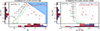Fig. 7

Left panel: rest-frame NUV-r⁺ versus r⁺ color-magnitude diagram for the z_spec members of the PCl J1001+0220 proto-cluster (red diamonds) and a matched coeval field sample at 4.23 < z < 4.88 (small navy dots) at stellar masses $\log (M_{*} / M_{⊙}) \geq 9.7$ $\log(\mathcal{M}_{\ast}/M_{\odot})\ge 9.7$ . The stellar mass cut is imposed here in an attempt to mitigate any induced differential bias between the field and proto-cluster members. Overplotted are the expected locations in this phase space of a progentor of a low-redshift cluster L^* galaxy (assuming passive evolution) estimated from synthetic spectra (see Sect. 4.2.1) at different stellar-phase metallicities and with different SFHs. The gray dashed track is generated from an instantaneous burst while the three green tracks are generated from an exponentially declining SFH with τ = 100 Myr at three different stellar-phase metallicities. Age ticks along each track indicate the time since the inception of the star formation event. Color and magnitude histograms for each sample are normalizedto each other such that they contain the same area. The solid light blue area indicates the area of this phase space for which VUDS is no longer representative of the underlying photometric sample at these redshifts and stellar masses (see Sect. 4.2.1). Right panel: rest-frame M_NUV - $M_{r^{+}}$ $M_{r^{+}}$ versus $M_{*}$ $\mathcal{M}_{\ast}$ color-stellar-mass diagram for the identical samples as in the left panel. The meanings of all symbols and lines are unchanged. While some of the brightest, reddest, and most (stellar) massive galaxies in the entire spectroscopic sample at these redshifts fall within PCl J1001+0220, only a moderately significant difference in the average brightness and a significant difference in the stellar mass distribution is detected relative to the coeval field population.

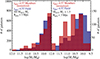Fig. 8

Left panel: histograms of stellar mass as estimated by LE PHARE for all z_phot members of the PCl J1001+0220 proto-cluster (left panel) and only those z_phot members with redder rest-frame colors ( $M_{N U V} - M_{r^{+}} > 1.5$ $M_{NUV}-M_{r^{+}}>1.5$ , right panel) plotted against the corresponding coeval field sample. Such a color cut selects galaxies with ages in excess of 200 Myr (see Fig. 7). All spectroscopic knowledge is ignored when defining these samples. Photo-z membership is defined by the projected radial cut given in the top left of the panel and 4.53 − 1.5σ_NMAD(1 + 4.53) < z_phot < 4.60 + 1.5σ_NMAD(1 + 4.60) with the remaining galaxies in this z_phot range comprising the coeval field sample. Histograms in both panels are normalized such that they contain the same area. While the two distributions shown in the left panel are formally consistent, once a color cut is imposed, the two distributions are found to be disparate at a >3σ level, with redder z_phot proto-cluster members exhibiting a preference for significantly higher masses relative to the coeval field.

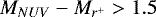
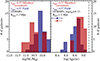Fig. 9

Left panel: distribution of stellar masses of spec-z members of PCl J1001+0220 (red histogram) and coeval field galaxies (blue histogram) as measured by GOSSIP+. The projected radial cut used to define membership is indicated at the top left of the panel. Right: distributions of the formation ages of proto-cluster spec-z members and coeval field galaxies, where age_f is defined as the time elapsed since the galaxy began forming stars (see Thomas et al. 2017b). Colors are identical to the left panel. The age of Universe at the redshift of the proto-cluster (z ~ 4.57) using our adopted cosmology is denoted by the dashed line. Two coeval field galaxies with log(age_f yr⁻¹) ~ 7.7 are not shown for clarity. Average effective 1σ lower and upper uncertainties for age estimates of the galaxies in each sample are shown in the top left. There is an obvious excess of more (stellar) massive and older galaxies within the bounds of the proto-cluster; both sets of distributions are inconsistent with being drawn from the same underlying population at a >2.5σ level and have average quantities which are inconsistent at an even larger significance. Additionally, the majority of proto-cluster members (5/9) appear to have formed within 500 Myr of the Big Bang as compared to only ~10% of coeval field galaxies.

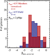Fig. 10

Distributions of the estimate for the index of the power-law dependence between flux density and wavelength in the rest-frame UV (β-slope) measured from the photometry of individual galaxies for PCl J1001+0220 spec-z members and the coeval field (red and blue histograms, respectively). Measurements are made assuming a single (unbroken) power-law dependence of f_λ on λ for each galaxy following the method of Hathi et al. (2016). For galaxies at z < 4.5, β is measured with the i⁺z⁺Y J photometry spanning roughly 1300 Å < λ_rest < 2300 Å. At z > 4.5, the i⁺ band is exchanged for the H band (covering roughly 1400 Å < λ_rest < 3000 Å) to prevent Lyα emission from potentially contaminating the measurement. The average errors on individual measurements for the two samples are shown at the top left (σ_β ~ 0.2 in both cases). Galaxies where extremely blue β-slopes are measured (β < −2.5) have average errors roughly twice the global average. The median β-slope for both samples is $\tilde{β} ~ - 1.7$ $\tilde{\beta} \sim-1.7$ and no significant difference is measured between the two distributions.

4.2.2 Multiwavelength properties and AGN content

One of the most intriguing lines of inquiry of high-redshift environmental studies relates to the question of whether the proto-cluster environment preferentially enhances, diminishes, or has no effect on the frequency and/or level of star formation and galactic nuclear activity in galaxies relative to matched samples in field environments. An overwhelming variety of results have been obtained for studies of high-redshift (proto-)clusters (e.g., Digby-North et al. 2010; Capak et al. 2011a; Martini et al. 2013; Cucciati et al. 2014; Lemaux et al. 2014a; Casey et al. 2015; Diener et al. 2015; Wang et al. 2016) underscoring that trends are highly dependent on the sample selected, the nature of the overdensity or overdensities studied, the level of care taken in appropriately matching the high- and low-density samples, and the wavelength of light and scheme used to proxy star formation or AGN activity. Though the amount of information available to us at z ~ 4.57 is somewhat limited, we draw here on nearly the entirety of the wealth of data in the COSMOS field to attempt to investigate the relative level of activity in the PCl J1001+0220 proto-cluster.

Shown in Fig. 11 are the LE PHARE SED-fit stellar masses and SFRs of the (z_spec) proto-cluster members plotted against those of the coeval field population subject to the constraints applied in the previous section. By eye, the two SED-fit SFR distributions appear similar, with a KS test confirming this observation, finding the two distributions to be statistically indistinguishable. As in the previous analyses, we do not rely solely on a KS test to attempt to distinguish the two populations. Shown in the top right-hand corner of Fig. 11 are the median SED-fit SFRs of each population along with their bootstrapped uncertainties generated following the method of Lemaux et al. (2014a). While there appears a slight suppression of the level of star formation activity within the proto-cluster bounds, the uncertainties are far too large to claim any level of significance. As all galaxies in VUDS are, by selection, star forming, these galaxy populations cannot be used to comment on the frequency (fraction) of star-forming galaxies in each environment. Similarly ambiguous results are found when we compare the star formation activity of the z_phot proto-cluster member sample relative to that of the z_phot coeval field sample. Using the definitions from Sect. 3.2 results in median SED-fit SFRs of 46 ± 12 and 32 ± 3 $M_{⊙}$ $\mathcal{M}_{\odot}$ yr⁻¹ for the z_phot proto-cluster member andcoeval field populations, respectively. A lack of significant differences in this quantity remains if we instead consider only those z_phot objects in the magnitude-color- $M_{*}$ $\mathcal{M}_{\ast}$ phase space where VUDS is representative (see Sect. 4.2.1).

The previous analysis relies on SED-fit SFRs, a method that has not been thoroughly tested for accuracy at the redshifts explored in this paper, a deficiency which is amplified due to the relatively small size of the galaxy samples considered here. Further, the SED-fit SFRs are extinction corrected using photometry that has only a modest dynamic range in wavelength in the rest-frame, the bulk of which lies in the rest-frame UV at these redshifts. As such, we attempt here to measure the average SFR of the proto-cluster member and coeval field samples using a tracer not subject to such uncertainties. Such a complementary approach is important as it has been suggested that at least some (proto-)clusters are dominated by dusty star-forming galaxies (e.g., Casey et al. 2015; Wang et al. 2016). For this purpose we are required to shift to wavelengths further to the red. There are only four viable possibilities for the COSMOS field. The first are deep Spitzer/MIPS 24 μm observations used to routinely probe galaxy populations at 0 < z < 2 in COSMOS (Le Floc’h et al. 2009). However, at z ~ 4.57, these observations are too far blue to reliably probe young stellar emission processed and re-radiated by dust. The second are deep Herschel/PACS and SPIRE observations taken on COSMOS, but even at z ~ 3, the stack of100s to 1000s of galaxies are needed for a significant detection (Álvarez-Márquez et al. 2016). The third comes from imaging taken with the James Clerk Maxwell Telescope (JCMT) at 850 μm to a 5σ depth of 6.0 mJy/beam observed as part of the SCUBA-2 Cosmology Legacy Survey (S2LCS; Geach et al. 2017). The final possibility comes from recently obtained extremely deep (currently 11.5 μJy/beam, 5σ) 3 GHz imaging from the Karl G. Jansky Very Large Array (JVLA) of the entirety of the COSMOS field (Novak et al. 2015; Smolčić et al. 2017b). The rest-frame frequency which these observations correspond to at z ~ 4.57 is a probe of synchrotron emission generated from supernovae and is found to correlate well with star formation activity (see Condon 1992 and references therein) in the absence of a radio AGN. The latter possibility is addressed later in this section. No significant individual detections in either the S2LCS nor the JVLA imaging were found amongst the proto-cluster member or coeval field samples.

In order to attempt to place more stringent constraints on the prevalence of dusty star formation activity we performed stacking on the JVLA imaging, which was preferred over the S2LCS imaging due to its comparable depth in SFR and considerably smaller PSF. Proto-cluster member and coeval field galaxies were stacked separately at 3 GHz by inverse-variance-weighted mean combining postage stamps centered on the optical centroid of each galaxy. While poor relative astrometry, if randomly rather than systematically poor, can render this exercise pointless, the astrometry of the JVLA mosaic was checked against the COSMOS2015 catalog and was found to be accurate to an RMS of 0.1′′. As this is half the size of the JVLA pixel scale and considerably smaller than the restored circular PSF of 0.75′′, it is unlikely that astrometric smearing would lead to degradation of any stacked signal. Despite the extreme depth of the data, the relatively large (combined) sample size, and the relatively high mean optical/UV SFRs estimated for each sample, in neither case was a significant (>3σ) detection measured. The 3σ f_ν limit for the proto-cluster member sample was found to be 2.24 μJy. This limit translates to a 3σ SFR_1.4GHz limit of <157 $M_{⊙}$ $\mathcal{M}_{\odot}$ yr⁻¹ following a k-correction of α =0.68 (Lemaux et al. 2014b) and the SFR conversion of Bell (2003) converted to a Chabrier (2003) IMF. This limit, overplotted in Fig. 11, is ~4× the average UV/optical SFR of the proto-cluster member sample. However, since this ratio is dependent on the dust-correction scheme employed by the SED fitting process, we instead calculate the IR excess (IRX ≡ L_IR∕L_FUV) from the average M_FUV and the radio limits assuming the q_TIR value from Lemaux et al. (2014b) for star-forming galaxies. This exercise yields an IRX ≲ 10 for the proto-cluster member sample, a value which precludes pervasive dusty starburst activity amongst the proto-cluster member galaxies. A similarly stringent limit of IRX ≲ 6 is found for the same sample if we replace the stacked radio limit with the L_IR limit as derived by MAGPHYS from the average proto-cluster member SED. An additional attempt was made to stack with Herschel/SPIRE but no significant detection was found and the corresponding limits were too shallow.

The 54 galaxies of the coeval field sample were stacked at 3 GHz in a similar manner finding no detection and resulting in a 3σ f_ν limit of 0.95 μJy or a SFR_{1.4 GHz, 3σ} limit of <64 $M_{⊙}$ $\mathcal{M}_{\odot}$ yr⁻¹ at z ~ 4.6. Such limits begin to rival the average UV/optical SFRs of the coeval field sample (see Fig. 11) and the resulting IRX limit of ≤4.8 approaches the value expected for galaxies with β slopes similar to those observed in the coeval field sample (e.g., Álvarez-Márquez et al. 2016). As above, a similarly stringent value of IRX ≤ 2 is found if we instead impose the MAGPHYS L_IR limit in conjunction with the average M_FUV. While not extremely constraining for the populations studied in this paper, this exercise has allowed us to definitively show that the SED-fit SFRs do not vastly underestimate the true SFRs for these populations and that, despite the high redshift and relatively high local densities, the proto-cluster is not dominated by dusty, prodigiously star-forminggalaxies, nor, for that matter, by radio AGN activity. However, neither this analysis nor the β-slope analysis presented in the previous section precludes the possibility that some subdominant portion of the member population is undergoing obscured star formation activity (as in, e.g., Hatch et al. 2017). Such analysis will be followed further as the member and coeval field sample in and around PCl J1001+0220 is increased and for other, lower redshift VUDS proto-structures discovered in the COSMOS field.

To investigate the relative presence of AGN activity amongst the proto-cluster member and coeval field populations we matched both samples to the Chandra-COSMOS point source catalogue (Elvis et al. 2009; Civano et al. 2016) finding no significant detection (>3σ). No significant detections were found amongst the z_phot proto-cluster members either. Such matching was also performed on the JVLA 3 GHz imaging finding no significant detection to a 3σ power density limit of log(P_ν W⁻¹ Hz)≳24.4. Additionally, Chandra images¹⁵ were stacked using the optical position of the sources as a centroid yielding no significant stacked signal to a 90% limit of log(L_{X, 2−−10 keV} ergs⁻¹ s) < 43.54 and 43.21 for the proto-cluster member and coeval field populations, respectively. An identical stack was performed on z_phot proto-cluster members yielding no significant detection to a depth of log(L_{X, 2−10 keV} ergs⁻¹ s) < 43.10. Note that the proto-cluster lies at the boundary between the deep and shallower portions of the C-COSMOS survey with the effective exposure times varying by a factor of ~5 over area enclosed by both the spectral and z_phot members. Further, we applied the mid-infrared criteria developed by Donley et al. (2012) to select powerful (both obscured and unobscured) AGN, finding that none of the sources analyzed here exhibit an AGN-like trend which could possibly be ascribed to a circumnuclear torus. Note that, in this context, the terms “obscured” and “unobscured” AGN refer to sources with rest-frame optical emission dominated by the host galaxy or by the AGN, respectively. The lack of individual and stacked X-ray and mid-infrared emission along with the complete absence of any broadline AGN activity amongst the VUDS sample at these redshifts suggest that no significant radiatively efficient AGN activity is taking place in these sources.

To test this hypothesis in a statistical sense, we constructed the average SED separately for the proto-cluster member, coeval field, and z_phot members. These average SEDs were then fit with SED3FIT (Berta et al. 2013) via $χ_{ν}^{2}$ $\chi_{\nu}^2$ minimization. Through this SED-fitting decomposition technique we found that the fraction of the rest-frame IR (8–1000 μm) and UV light contributed by the torus/AGN is, in all three cases, negligible (≤1%). In the mid-IR, defined as an integration over 5–40 μm in the rest-frame, where the relative contribution from an obscured AGN is maximized, the fraction of light contributed by the torus/AGN remains at only a few percent (≤5%). This line of analysis, while almost certainly imprecise due to only upper limits being available on many of the most discriminating bands, allows us to make definitive claims on the prevalance of AGN activity amongst the proto-cluster galaxies. It appears that, within the limits of our data, there is no evidence for any powerful (i.e., quasar level) unobscured or obscured radiatively efficient or inefficient AGN activity in any of the known or potential member galaxies, a conclusion which is robust to changes of factors of a few in the above estimates. This fact precludes the possibility that such activity is a requisite condition for the presence of a proto-cluster and suggests that the proto-cluster does not necessarily foster such activity (e.g., Hatch et al. 2014), though the validity of the latter suggestion is subject to a variety of timescale concerns which we do not attempt to address in this paper.

As a final thought related to multiwavelength activity in and around PCl J1001+0220, it is interesting to note that a prodigiously star forming submillimeter galaxy (SMG, SFR_TIR = 500–2000 $M_{⊙}$ $\mathcal{M}_{\odot}$ yr⁻¹) or galaxy–galaxy merger detected in AzTEC 1.1 mm observations was spectroscopically confirmed by Capak et al. (2008) to be at z = 4.547 ± 0.002, in proximity to PCl J1001+0220. Such a discovery is interesting since potential links between proto-structures and SMGs have been proposed by many authors (e.g., Daddi et al. 2009; Aravena et al. 2010; Smolčić et al. 2017a; Wilkinson et al. 2017). However, this SMG is well outside the bounds of either the z_spec or z_phot proto-cluster member samples ([α_J2000, δ_J2000] = [150.22715, 2.5764]) regardless of the choice of centers. As a consequence, PCl J1001+0220 could not have been found solely by looking for an overdensity surrounding this SMG. While the SMG may eventually merge with the proto-cluster core, a process that would take ~6 Gyr assuming the LOS velocity to be equivalent to the infalling velocity and a purely radial orbit, it is sufficient to say that the proto-cluster and the SMG do not appear causally related at the epoch at which they are observed.

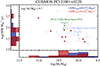Fig. 11

Distribution of the PCl J1001+0220 spec-z members (red diamonds and histogram) and coeval field galaxies (navy points and histogram) in the SFR- $M_{*}$ $\mathcal{M}_{\ast}$ plane as estimated by LE PHARE. Histograms are normalized as in other figures such that the area is identical for both samples. The upper limit to the radio-derived SFR of spec-z member and coeval field galaxies coming from stacked 3 GHz JVLA data is shown as the green and light blue lines/arrows, respectively. The lack of detection for both proto-cluster members and coeval field galaxies suggests that prodigious dusty star formation (IRX ≲ 10) is no more common in the proto-cluster than in the overall field at these redshifts and is not particularly common in either environment.

4.2.3 Morphological properties

In the penultimate section of the comparisons between proto-cluster members and coeval field galaxies we return to rest-frame UV light to inspect the morphology of these galaxies as they appear in the COSMOS HST/F814W imaging. Because the PCl J1001+0220 is not covered by the CANDELS/COSMOS survey, these images are the only images for which we can get reliable morphological information. This band is nearly identical to the rest-frame FUV at these wavelengths¹⁶ and, thus, any morphological information derived from these images will be highly subject to dust effects. While we showed earlier in Sect. 4.2.1 that there does not appear to be any bulk difference between the two populations in this regard in terms of integrated dust content, differing dust geometry may still differentially affect the measurements of the two samples. As such, we limit ourselves here to the most basic of morphological quantities and observations.

Plotted in Fig. 12 are the HST/F814W postage stamps of the nine PCl J1001+0220 member galaxies. Given in the bottom left-hand corner of each postage stamp is the effective circularized radius (r_e,circ) obtained from GALFIT for each galaxy following the methods of Ribeiro et al. (2016). Proto-cluster members are observed to span a wide variety of FUV morphologies from irregular diffuse galaxies with multiple clumps to compact, high surface-brightness galaxies. Correspondingly, the observed r_e,circ values span nearly an order of magnitude from 0.3 to 2.2 kpc with an average of 1.2 kpc. The (luminosity-)dominant stellar populations probed in these images are those associated with the current star formation activity in member galaxies. Thus, the vast diversity of morphologies and r_e,circ values unambiguously demonstrate that while these galaxies appear to share a common overarching environment, their stellar mass assembly is not proceeding in a common manner. This large variety of visual morphologies and r_e,circ values is, however, also shared by the general VUDS field population at these redshifts (Ribeiro et al. 2016). While it should be noted that a stellar mass limit was imposed on the sample in Ribeiro et al. (2016), this imposition was only made on galaxies in their lower redshift bins meaning that the galaxies in redshift bin referenced here, 3.5 ≤ z ≤ 4.5, the highest redshift studied in Ribeiro et al. (2016), can be validly compared to the coeval field sample. Such a large diversity in UV morphologies in all cases is perhaps not unexpected for galaxies at these redshifts as either continuous moderate-level (~20 $M_{⊙}$ $\mathcal{M}_{\odot}$ yr⁻¹) or shorter-lived, vigorous star formation over the course of the last ~1 Gyr is required to build up the average stellar mass of member and coeval field galaxies.

While the same range in visual and (one form of) parametric morphologies is observed in both the coeval field and the proto-cluster member population, the latter has a σ_NMAD ~ 25% higher and in a sample comprised of only nine galaxies. To test the likelihood of the dispersion in the observed size distributions occurring by random sampling of the VUDS field galaxies at this redshift, we randomly drew 1000 samples of nine galaxies from the r_e,circ distribution observed in Ribeiro et al. (2016) for the redshift bin most comparable to our own. In only ~10% of the trials did the variance of the r_e,circ values in the randomly drawn sample exceed that of the proto-cluster member sample. This result is identical if we instead perform this exercise drawing from a Gaussian fit to the distribution of r_e,circ values of the coeval field sample. However, because galaxy size is correlated with the mass of their stellar content (e.g., Allen et al. 2015), it is perhaps the potentially disparate stellar mass distribution of the member population with respect to the field that drives the observed scatter (see Sect. 4.2.1). Further, the lack of an azimuthally symmetric profile for a large fraction of both the member and coeval field samples, a phenomenon common to galaxies at high redshift (e.g., Mortlock et al. 2013; Guo et al. 2015), likely decreases the utility of both the r_e,circ measurement and the scatter on this quantity. To mitigate both issues, an effective non-parametric half-light radius, $r_{T}^{50}$ $r^{50}_{T}$ , was measured for each galaxy in both the member and coeval field samples following the methodology of Ribeiro et al. (2016) and normalized in such a way as to remove the correlation between size and stellar mass (see Fig. 13). None of the results in this section change appreciably if we instead adopt $r_{T}^{100}$ $r^{100}_{T}$ , the effective non-parametric radius containing 100% of the flux of each galaxy. Performing a similar exercise as was done for the r_e,circ distributions again on those of $r_{T}^{50} / M_{⋆}^{α}$ $r^{50}_{T}/M_{\star}^{\alpha}$ results in ~10% of trials exceeding the observed variance of proto-cluster member population, a result which mildly suggests more stochasticity in the assembly stage of member galaxies relative to the field.

Assuming this increased scatter to be real, we explore here the possibility of increased galaxy–galaxy interactions and potential merging activity within the proto-cluster as possible driving mechanisms for this increased stochasticity. In order to estimate the level and type of galaxy–galaxy interactions experienced by the average galaxy in the member and coeval field samples, for each galaxy in each sample we counted the number of unique objects in the magnitude range 24 ≤ F814W ≤ 26 other than the galaxy itself whose centroids lay within r_proj < 25 kpc from the galaxy center. This radius was adopted as it is commonly used for galaxy pair studies and has been found through simulations and observations to contain galaxies with a high likelihood of eventual coalescence (see e.g., Le Fèvre et al. 2000; de Ravel et al. 2009; Lotz et al. 2011; López-Sanjuan et al. 2013, 2015 and references therein). It is worth noting that galaxy–galaxy interactions can have visible effects over much larger separations (r_proj ~ 50–100 kpc, e.g., Patton et al. 2011) and can still merge given a long enough timescale (3–8 Gyr, Kitzbichler & White 2008). Here, however, we are concerned only with the most severe of interactions and thus limit ourselves to the more restrictive criterion. The bright end of the magnitude limit imposed corresponds to M_FUV≲ − 22.3 at z ~ 4.5 (~3L^*), a population extremely unlikely to be observed with any abundance in the small areas searched here (Bouwens et al. 2015). The fainter end of the magnitude range given above was set as a rudimentary attempt to control for surface brightness effects and detection limits as F814W ~ 26 corresponds to the 50% completeness limit for r_h = 0.25′′ sources (Scoville et al. 2007a). Finally, because the ACS observations probe the rest-frame FUV, there is some concern that confusion could occur between multiple distinct galaxies and bright star-forming regions contained within a single galaxy. The method for disambiguating these cases in VUDS is discussed in detail in Ribeiro et al. (2017).

Subsequent to these cuts, the simplest possible comparison is made: the average number of companions per galaxy in the two samples corrected by the average density of sources in this magnitude range in the COSMOS2015 catalog. In total, 0.4 ± 0.3 and 0.1 ± 0.1 background-corrected projected companions per galaxy are found for the proto-cluster member and coeval field sample, respectively. A discrepancy of similar directionality and significance is seen when comparing the z_phot member and field sample,0.17 ± 0.08 versus 0.08 ± 0.02, respectively. While these results depend on the choice of the magnitude and r_proj criteria adopted, the cuts chosen here are the most conservative that could be made with respect to projection effects for which this analysiscould reasonably be performed. For these choices, the analysis is suggestive of possible elevated levels of strong galaxy–galaxy interactions within the proto-cluster bounds. This line of thought will be followed further at the conclusion of future followup spectroscopic observations of this and other VUDS proto-clusters.

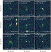Fig. 12

Hubble/ACS F814W 5 × 5′′ (~ 33 × 33 kpc) postage stamps of the nine secure spec-z members of PCl J1001+0220. At the redshift of the proto-cluster, F814W almost exactly corresponds to the rest-frame FUV band. The redshift, SFR, circularized effective radius (r_e,circ), and stellar mass for each galaxy is shown in each panel. The nine galaxies exhibit a large diversity of morphologies, from a single, compact (r_e,circ < 0.5′′) bright star-forming clump to larger (r_e,circ ~ 1 − 2′′), multi-component diffuse structures devoid of concentrated light. Many of the proto-cluster members are observed with single or multiple projected companions, a rate which possibly exceeds that of the coeval field (see text).

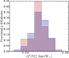Fig. 13

Distribution of non-parametric total sizes, $r_{T}^{50}$ $r_{T}^{50}$ , as measured in the Hubble/ACS F814W imaging of spec-z member galaxies of PCl J1001+0220 compared to that of the coeval (red and blue histograms, respectively). As in previous figures, histograms are normalized to have equal areas. Due to the relationship between size and stellar mass, size measurements are modulated by the estimated stellar mass of each galaxy ( $M_{⋆}^{α}$ $M_{\star}^{\alpha}$ ) where α is derived from a fit to the observed size-stellar mass relation in the combined proto-cluster and coeval field sample (α = 0.18 ± 0.03). The average value for both samples is identical within the uncertainties, though a slight increase (~25%) in the spread of the proto-cluster distribution is observed which we argue in Sect. 4.2.3 that, if real, may be due to increased galaxy–galaxy interactions.

4.2.4 Spectral properties

The final comparison between proto-cluster members and their field counterparts comes in measuring rudimentary individual and stacked (hereafter “coadded”) spectral properties. We begin with the former and concentrate on the features most commonly studied for high-redshift galaxies. The Lyα feature has been found to have a complex relationship with environment in the few studies with a reasonable chance to test this possibility. In some cases an enhancement of the Lyα feature has been found. Larger Lyα-emitting regions were found to be associated, on average, with Lyα emitters (LAEs) situated in overdense environments (Matsuda et al. 2012; Momose et al. 2016; Chiang et al. 2015). It has been suggested that the presence of such overdensities are possibly a requisite condition in the higher redshift Universe in order to observe multiple strong, physically associated LAEs (e.g., Castellano et al. 2016). Indeed, some proto-cluster or proto-cluster candidates have been found solely through the presence of large numbers of relatively strong LAEs (e.g., Pentericci et al. 2000; Venemans et al. 2002; Kuiper et al. 2011; Chiang et al. 2015) with some studies finding an increase of strong narrowband-selected LAEs with increasing local galaxy density (e.g., Zheng et al. 2016). Such an increase in the size of Lyα halos could be related to both the column density and kinematics of the neutral hydrogen in and around the galaxies (see Guaita et al. 2017 and references therein) and, thus, a possible signature of a nascent medium.

However, other results have found a lack of enhancement or suppression of Lyα amongst galaxies in the higher-density environments. Narrowband-selected LAEs are found in general to be less clustered than those galaxies without strong Lyα emission at high redshifts (e.g., Ouchi et al. 2010; Bielby et al. 2016), though this trend is predicted to be a strong function of redshift and Lyα line luminosity (Orsi et al. 2008). In a study of the member galaxies of a z ~ 3.3 proto-cluster, Lemaux et al. (2014a) found no definitive evidence for differences in individual or coadded Lyα measurements compared to a corresponding coeval field population. In a study of a narrow-band-selected z = 3.78 proto-cluster, Dey et al. (2016) found no environmental dependence of EW(Lyα) between proto-cluster LAE candidates and coeval field candidate LAEs, though a marginal increase in the average Lyα luminosity was seen closer to the core of the proto-cluster. In a spectroscopic study of a proto-cluster LAEs at z ~ 3.67, Toshikawa et al. (2016) found proto-cluster member galaxies to exhibit less negative EW(Lyα) relative to galaxies in a similarly selected field sample indicating a suppression of the Lyα escape fraction in the proto-cluster.

Here we attempt two basic comparisons. In the first comparison we plot in the left panel of Fig. 14 the coadded spectrum of all nine PCl J1001+0220 members against that of the coeval field sample. These coadded spectra are generated following the methodology of Lemaux et al. (2014a) and show the unit-weighted (normalized) average (mean) spectra of the two populations. The wavelength region in the left panel of Fig. 14 is tailored such that only those wavelengths where all galaxies contribute the coadded spectra for each population are shown. Immediately it can be seen that, while the overall continuum shape is similar between the two coadded spectra, a fact which bolsters the β-slope analysis presented in Sect. 4.2.1, there appears a noticeable difference in the strength of the emission component of the Lyα line. We use a custom bandpass IDL routine to measure the EW(Lyα) of both coadded spectra, which, similarly to Cassata et al. (2015), uses the continuum just redward of Lyα to set the continuum level. For individual measurements of EW(Lyα), this routine returns measurements which are broadly consistent with those of Cassata et al. (2015). Using this method we measure EW(Lyα) = − 4.7 ± 0.6 and − 15.4 ± 0.3 Å for the proto-cluster member and coeval field galaxies, respectively. We note that these cannot be directly compared to the mean values of the individual measurements due to the fact that each spectrum has its average flux density scaled to unity prior to coadding. Uncertainties on mean EWs are derived from a combination of the covariance matrix of the linear continuum fit and the error spectrum of the coadded spectra constructed from the individual VIPGI error spectra of the input galaxies. Though there are some known issues with the latter, neither EWs or their associated uncertainties are found to change significantly if a running measure of the root mean square fluctuations is instead used. The suppression of Lyα relative to the level of the UV continuum amongst the proto-cluster galaxies is clearly significant, a difference which persists in significance and directionality if we instead perform unit-weighted median coadding. In the right panel of Fig. 14 we plot the distributions of the individual measurements of EW(Lyα) as measuredby Cassata et al. (2015) for the proto-cluster member and coeval field samples used to construct the coaddedspectra. By eye it appears that the proto-cluster members are skewed to less negative EW(Lyα) values with respect to those of the coeval field sample, an observation which is borne out both by a KS test (rejection of null hypothesis at ~99%) and by a comparison of the mean values (−5.5 vs. −37.6 Å, respectively).

It is important to note, though, that, as we do not preserve flux density in our coaddition method, this suppression cannot necessarily be interpreted as a suppression of Lyα line luminosity. For this to also be true, the dust-uncorrected FUV luminosity between the two samples must be similar. Both a KS test and a comparison of the average of the M_FUV values of the proto-cluster member and coeval field galaxies ( $\tilde{M_{F U V}} = - 21.77 \pm 0.18$ $\tilde{M_{FUV}}=-21.77\pm0.18$ and − 21.60 ± 0.06, respectively) show no significant offset between the two samples. Echoing this result, a KS test performed directly on the Lyα line luminosity measurements, made following the method of Cassata et al. (2015), rejects the hypothesis that the two distributions are drawn from the same underlying parent sample at >99%. It appears that the suppression of Lyα relative to the UV continuum observed in the proto-cluster members relative to the coeval field galaxies extends to an absolute suppression of Lyα luminosity. Given that the two populations appear to have similar dust properties and UV-derived SFRs, and because the absolute brightness of Lyα in the absence of resonant scattering and dust is directly proportional to the amount of star formation, this decrease can be translated directly into the fraction of Lyα photons which escape the average galaxy in the two populations. Adopting the Lyα SFR conversion of Lemaux et al. (2009) with no correction for intergalactic medium absorption, converting to a Chabrier (2003) IMF, and replacing L(Lyα) with a combination of EW(Lyα) and M_FUV gives: $S F R (L_{Ly α}) = - 8.6 \times 10^{9} (10^{\frac{- (〈 M_{F U V} 〉 + 48.6)}{2.5}}) 〈 E W (Ly α) 〉 M_{⊙} {yr}^{- 1},$ $\begin{equation*} SFR(L_{\textrm{Ly}\alpha}) = -8.6\times10^{9} (10^{\frac{-(\langle M_{FUV} \rangle +48.6)}{2.5}}) \langle EW(\textrm{Ly}\alpha) \rangle \, \mathcal{M}_{\odot} \, \textrm{yr}^{-1},\\\end{equation*}$ (4)

where M_FUV is the (linear) average M_FUV of the sample, ⟨EW(Lyα)⟩ is measured in the coadded spectra, and the constant of proportionality comes from a combination of that given in Lemaux et al. (2009), 4 $π d_{L}^{2}$ $\pi d_{L}^2$ , where d_L is 10 pc in cm, c is cm s⁻¹, and the λ_eff of the FUV filter (1539 × 10⁻⁸ cm, Boselli et al. 2011). We then define the escape fraction of Lyα as: $f_{e s c, L y α} = S F R (L_{Ly α}) / S F R_{S E D},$ $\begin{equation*} f_{esc, \, Ly\alpha}= SFR(L_{\textrm{Ly}\alpha})/SFR_{SED},\\\end{equation*}$ (5)

where the SFR_SED are the average values given in Sect. 4.2.1. For the full VUDS sample in COSMOS at 2 ≤ z ≤ 5 with flags ≥X2 we have confirmed that, as EW(Lyα) becomes more negative, that is, more Lyα flux for a given UV continuum level, f_{esc, Lyα} approaches 100% using the above formalism. The resulting values for the proto-cluster member and coeval field sample are $f_{e s c, Ly α} = {1.8}_{- 1.7}^{+ 0.3}$ $f_{esc, \, \textrm{Ly}\alpha} = 1.8^{+0.3}_{-1.7}$ % and ${4.0}_{- 0.8}^{+ 1.0}$ $4.0^{+1.0}_{-0.8}$ %, respectively. The coeval field value is broadly consistent with the global f_{esc, Lyα} at 4 < z < 5 as derived through comparisons between Lyα and UV luminosity functions (Hayes et al. 2011; Zheng et al. 2013) or other measures (e.g., Wardlow et al. 2014; Cassata et al. 2015 though these measurements were limited to LAEs only), especially considering the unknown uncertainties of differing sample selections and measurement schemes. The average f_{esc, Lyα} for proto-cluster members appears, however, at the extreme low end of measured values at these redshifts.

A variety of factors can increase the chance of the escape of Lyα photons or the appearance thereof: geometric effects, observational bias, dust content and geometry, strong outflows, and decreased column densities of neutral hydrogen along the line of sight. Because we are averaging over a reasonably large number of galaxies in each sample, geometrical effects (see e.g., Finkelstein et al. 2008), are likely not the cause of the observed difference. Similarly, because we are comparing galaxy samples with the same mean redshift observed in an identical manner, it is unlikely that differing measurement apertures, a pernicious effect when measuring f_{esc, Lyα} (e.g., Matthee et al. 2016), affect our measurements here. Further, we have shown through a variety of methods that the dust content between the two samples is likely to be the same. Therefore, we are left with only two possibilities: increased prevalence and strength of outflows amongst the coeval sample or decreased H I column density. It has been shown that the presence of outflows and their strength depend, in the absence of strong AGN activity, on the instantaneous SFR (e.g., Heckman 2001; Weiner et al. 2009; Erb 2015), a quantity which, as far as we can tell, is the same between the two samples. In addition, we see no difference in the velocity offset of the Lyα line in the coadded spectra with respect to the ISM lines, 310 versus 270 km s⁻¹ for the coeval field and proto-cluster member coadded spectra, respectively, which suggests similar H I kinematics between the two galaxies. However, this test is far from definitive as the relationship between these components is not necessarily straightforward (e.g., Shapley et al. 2003; Guaita et al. 2017).

What remains, then, is the intriguing possibility that the proto-cluster galaxies see a denser medium in their immediate vicinity or a more isotropic medium resulting in a higher covering fraction of H I. Such conditions would cause a subsequent drop of Lyα photons able to escape (e.g., Reddy et al. 2016) due to their increased possibility of interacting with a dust grain for a given dust content and geometry. The presence of a large and dense neutral medium is a possibility which has been raised previously with the observation of large scale Lyα absorption in another VUDS proto-cluster (Cucciati et al. 2014) and in Lyα tomography studies (e.g., Lee et al. 2016) and is consistent with the idea of the assembly of a nascent proto-ICM. Assuming a one-to-one correspondence between increased H I and an increase in heavy elements, the possibility of denser medium is also broadly consistent with the relative strength ISM absorption features, as the average ratio between EWs measured on the proto-cluster member and coeval field coadded spectra for the six ISM absorption features labeled in Fig. 14 is 1.7 ± 0.2, measured using the bandpass method of Lemaux et al. (2010) with custom bandpasses. From comparing Gaussian fits to each of the features in the two coadditions we find that the increase in the average EW is driven almost entirely by an increased (relative) depth of theabsorption feature rather than by an increase in the feature width. Since all ISM features should be unresolved in VUDS data, this lack of appreciable difference in the widths measured in the ISM features of the two coadded spectra strongly indicates that the increased absorption strength in the cluster member coadded spectrum is real. However, the relationship between ionic column density and ISM absorption strength is a complicated one (see Talia et al. 2012 and references therein) and, as such, while suggestive, these measurements do not offer definitive proof that the galaxies inhabiting the proto-cluster are experiencing a denser medium. Such lines of inquiry will continue to be followed for the entire sample of VUDS proto-structures. It may be, though, that observations of cold gas from, for example, the Atacama Large Millimeter/submillimeter Array will be needed to definitively confirm or deny this assembly, a prospect which may have already begun to be realized (Ginolfi et al. 2016; Dannerbauer et al. 2017).

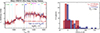Fig. 14

Left panel: unit-weighted (normalized) mean rest-frame VUDS spectra of the nine spec-z members ofthe PCl J1001+0220 proto-cluster plotted against that of the 53 coeval field galaxies (one galaxy was removed due to the presence of severe reduction artifacts). The requisite stellar mass limit for each coaddition is given in the figure panel. Each spectrum is smoothed with a Gaussian of FWHM = 1.5 pixels (1.45 Å). Important absorption and emission features frequently observed in VUDS spectra are marked by vertical lines. Clear differences can be observed between the two spectra, with the proto-cluster members exhibiting, on average, reduced Lyα emission andexaggerated absorption in Hydrogen and various metal lines relative to the average coeval field galaxy. In both cases, a significant (~300 km s⁻¹) offset to the red can be seen for the Lyα line potentially indicating that large-scale outflows are pervasive in galaxies at this redshift. Right panel: distribution of rest-frame Lyα equivalent widths (EWs) for the proto-cluster (red histogram) and coeval field sample (blue histogram) measured on individual spectra. Negative or positive EW indicates the line is seen in emission or absorption, respectively. The two distributions are inconsistent at >3σ, the Lyα feature being more likely to be seen in absorption for the proto-cluster members.

5 Summary and conclusions

In this study we reported on the detection, spectroscopic confirmation, and the mapping of the PCl J1001+0220 proto-cluster at z ~ 4.57 in the COSMOS field. We undertook a preliminary investigation of various properties of the spectroscopic and photometric proto-cluster member galaxies and contrast these with matched field samples. The following were the main conclusions of these investigations:

PCl J1001+0220 was discovered in a blind spectroscopic survey without the use of traditional beacons of proto-structure or proto-cluster activity such as quasars or other prodigious radio emitters. Its large extent on the plane of the sky is consistent with both predicted and observed sizes of high-redshift proto-clusters.
The galaxy overdensity of the proto-cluster was measured using three methods: spectroscopic overdensity, photometric redshift overdensity, and a new method, Voronoi Monte-Carlo mapping, which statistically combines both the spectroscopic and photometric redshifts. While the level of overdensity was found to be dependent on the method, in all three methods PCl J1001+0220 was significantly detected. The overdensity derived from the Voronoi Monte-Carlo mapping was considered the most secure, with PCl J1001+0220 exhibiting an average δ_gal = 3.30 ± 0.32 over a sky area of 7.58 Mpc² and a line-of-sight distance of 7.49 Mpc.
Several methods were attempted to measure the total mass associated with PCl J1001+0220. Though subject to a large number of assumptions and uncertainties, this analysis provided a general picture that PCl J1001+0220 will evolve into a cluster of mass ~3–10 × 10¹⁴ $M_{⊙}$ $\mathcal{M}_{\odot}$ by the present day, with the mass estimated from the overdensity derived from the Voronoi Monte Carlo approach falling at the low end of these estimates.
When comparing various member populations to similarly selected coeval field samples we found tentative evidence for a fractional excess of older and more massive galaxies within the proto-cluster bounds suggesting that the SFHs of galaxies in the proto-cluster environment differ appreciably, on average, from those in the field.
A variety of methods were used to attempt to quantify the level of AGN activity amongst the various member samples using some of the deepest multiwavelength data ever compiled. In contrast with studies of many other high-redshift proto-clusters, no indication was found for the presence of any type of AGN within the proto-cluster.
No evidence was found for either suppression or enhancement of star formation activity within the proto-cluster bounds through comparison of dust-corrected rest-frame UV star-formation indicators. Through cross-matching and stacking newly obtained deep JVLA 3 GHz imaging of the COSMOS field for both the proto-cluster member and coeval field samples it was demonstrated that neither environment contained a large number of dusty starbursting galaxies. Limits on the stacking analysis and the distribution of measured β slopes precluded the possibility of copious amounts of dust in the average galaxy in both populations.
The rest-frame FUV morphologies from the HST/F814W mosaic of the COSMOS field for the proto-cluster member and coeval field population were compared visually, parametrically, and non-parametrically. The nine z_spec membersspanned the entirety of all quantifiable morphological measurements of the corresponding coeval field sample which suggested, in tandem with a possible increase in the average number of background-corrected close pairs in both the z_spec and z_phot member sample, a potential enhancement of galaxy–galaxy interactions within the proto-cluster.
The individual and stacked spectral properties of the member and coeval field galaxies were contrasted. The member population exhibited a decided suppression in the strength of the Lyα emission feature relative to the coeval field as well as a decrease in the estimated average Lyα escape fraction ( ${1.8}_{- 1.7}^{+ 0.3}$ $1.8^{+0.3}_{-1.7}$ % vs. ${4.0}_{- 0.8}^{+ 1.0}$ $4.0^{+1.0}_{-0.8}$ %, respectively). Additionally, the average absorption of ISM features in the stacked spectra was markedly stronger for the proto-cluster members. These lines of evidence were used to suggest the possible presence of a large and dense medium housed in the proto-cluster.

Despite the relatively small sample assembled here, the observed properties of galaxies in PCl J1001+0220 tentatively demonstrate that local environment may already impact galaxy evolution and that the effects which give rise to the massive quiescent galaxies that dominate local galaxy clusters may begin to be felt as early as just 1.3 Gyr after the Big Bang. Further, the simple presence of PCl J1001+0220 and the inference of the large amount of mass assembled in the proto-cluster by z ~ 4.57 is a clear indication that such overdensities were able to begin to distinguish themselves from average density regions of the Universe well before the end of the epoch of reionization. While the existence and nature of PCl J1001+0220 was proven definitively in this study, many of the results pertaining to galaxy evolution within PCl J1001+0220 presented in this work do not have the statistical weight to be anything other than suggestive. That we were able to even attempt such lines of analysis in some sort of controlled manner at these redshifts already constitutes a triumph. It will be up to further spectroscopic observations of PCl J1001+0220, followup observations at other wavelengths, and future works using the full power of the VUDS survey or other large-scale spectroscopic surveys, such as the Subaru Prime Focus Spectrograph Galaxy Evolution Survey, to determine whether the tentative signs of early-onset environmentally driven evolution seen here are legitimate hallmarks of the general population of high-redshift proto-clusters.

Acknowledgements

This work was supported by funding from the European Research Council Advanced Grant ERC-2010-AdG-268107-EARLY and by INAF Grants PRIN 2010, PRIN 2012 and PICS 2013. This work was additionally supported by the National Science Foundation under Grant No. 1411943 and NASA Grant Number NNX15AK92G. VS, ID and MN acknowledge the European Union’s Seventh Framework programme under grant agreement 337595 (ERC Starting Grant, “CoSMass”). We thank Thibaud Moutard, Iary Davidzon, Lori M. Lubin, and Adam R. Tomczak for their insight relevant to the various analyses presented in this paper and their willingness to impart it through conversation. We also thank Conor Mancone and Anthony Gonzalez for their support with EZGAL under circumstances that made such support difficult and Clotilde Laigle for generously providing access to the COSMOS2015 catalog at an early stage of this work, a gesture which immensely helped its development. BCL thanks Pol Mollitor and Matvey Sapunov for providing the finest of company during the entirety of this work and for continually helping to create the destruction necessary, amongst other things, to write. This work is based, in part, on observations made with the Spitzer Space Telescope, which is operated by the Jet Propulsion Laboratory, California Institute of Technology under a contract with NASA. The scientific results reported in this article are also based in part on observations made by the Chandra X-ray Observatory and data obtained from the Chandra Data Archive. We thank ESO staff for their continuous support for the VUDS survey, particularly the Paranal staff conducting the observations and Marina Rejkuba and the ESO user support group in Garching.

Appendix A COSMOS multiwavelength imaging data

The COSMOS field, selected initially for its equatorial location, paucity of bright foreground objects, and extremely low Galactic extinction, first began to distinguish itself more than a decade ago following anunprecedented campaign with the Hubble Space Telescope (HST) which resulted in a 1.64 □° mosaic of the field compiled from 583 single-orbit pointings (5σ depth m_F814W ~ 27.2) with the Advanced Camera for Surveys (ACS; Ford et al. 1998) in the F814W band (Scoville et al. 2007a; Koekemoer et al. 2007). In parallel, a 1 □° overlapping sub-section of the field was selected to be the second deep field (D2) of the Canada-France-Hawaii Telescope Legacy Survey (CFHTLS¹⁷) which was, in conjunction with a proprietary campaign (Boulade et al. 2003), to eventually provide imaging in u^* ∕g′∕r′∕i′∕z′ to a 80% point source completeness depth of 26.26/26.31/25.91/25.51/25.14¹⁸, respectively, under exquisite conditions (median seeing 0.58′′). These two datasets would form the basis to motivate the subsequent training of almost every major telescope on the field, including:

At radio wavelengths (10–90 cm) with the Very Large Array (Schinnerer et al. 2007, 2010; Smolčić et al. 2014), the Giant Metrewave Radio Telescope (Smolčić et al. 2015; Karim et al. in prep.), and the Jansky Very Large Array¹⁹ (Novak et al. 2015; Smolčić et al. 2017b) to 5σ depths ranging from ~11.5–400 μJy/beam (from 10 to 90 cm, respectively).
In the far-infrared (FIR; 100–500 μm) with the Herschel space observatory (Pilbratt et al. 2010) Photodetector Array Camera and Spectrometer (PACS; Poglitsch et al. 2010) as part of the PACS Evolutionary Probe (PEP; Lutz et al. 2011) and Spectral and Photometric and Imaging REceiver (SPIRE; Griffin et al. 2010) as part of the Herschel Multi-tiered Extragalactic Survey (HerMES; Oliver et al. 2012) to 3σ depths of 4.5, 10.0, 18.4, 19.3, & 21.2 mJy (including confusion noise) in the 100, 160, 250, 350, & 500 μm channels, respectively.
In the near-, mid-, and far-infrared (3.6–160 μm) with the all seven channels of the Spitzer InfraRed Array Camera (IRAC; Fazio et al. 2004) and Multiband Imaging Photometer for Spitzer (MIPS; Rieke et al. 2004) for the COSMOS Spitzer survey (S-COSMOS; Sanders et al. 2007) to 5σ depths of 24.0, 23.5, 22.0, 21.2, & 19.0 mags in the [3.6], [4.5], [5.8], [8.0], & 24 μm bands, respectively, and, recently, extremely deeply in the non-cryogenic IRAC bands as part of the Spitzer Large Area Survey with Hyper-Suprime-Cam (SPLASH; Laigle et al. 2016) to 3σ depths of ~25.4 in the both the [3.6] and [4.5] bands.
In the near-infrared (NIR) Y∕J∕H∕K_s bands (1.0–2.1 μm) as the subject of the UltraVISTA survey (McCracken et al. 2012) to 3σ depths of m_AB ~ 24.5 in the “Deep” 0.88 □° region of the survey and m_AB ~ 25 in the smaller 0.62 □° “UltraDeep” portion of the survey, manifest as a series of four equally spaced and almost equally sized N-S vertical strips.
A small sub-section of the field (0.056 □°) in the optical/NIR (0.6–1.6 μm) as part of the Cosmic Assembly Near-infrared Deep Extragalactic Survey (CANDELS; Grogin et al. 2011; Koekemoer et al. 2011) to 5σ depths of28.2, 28.4, 27.0, and 26.9 in the F606W, F814W, F125W, and F160W bands, respectively.
At optical wavelengths (0.4–0.9 μm) with Subaru/Suprime-Cam employing a large variety of narrow, medium, and broadband (B∕V∕r⁺∕i⁺∕z⁺) filters (Taniguchi et al. 2007) as well as new imaging in z⁺⁺ as part of the SPLASH survey reaching 5σ depths of ~26–27 mags in all broadbands and ~25–26 mags in all medium/narrow bands.
In the ultraviolet (UV) with both channels (1500–2300 Å) of the GALaxy Evolution eXplorer (GALEX; Martin et al. 2005) to 3σ depths of25.8 and 25.5 in the far-UV (FUV) and near-UV (NUV) bands, respectively (Zamojski et al. 2007).
With the X-Ray Multi-mirror Mission space telescope (XMM-Newton; Jansen et al. 2001) as the subject of the XMM-COSMOS survey (Cappelluti et al. 2009; Brusa et al. 2010) and the Chandra X-ray observatory Advanced CCD Imaging Spectrometer (ACIS; Garmire et al. 2003) as the subject of the Chandra COSMOS survey (C-COSMOS; Elvis et al. 2009) and the more recent Chandra COSMOS-Legacy Survey (Civano et al. 2016) to ~3σ point source depths ranging from 4 × 10⁻¹⁶ − 1 × 10⁻¹⁴ ergs s⁻¹ cm² depending on the band and the telescope.

As well as a variety of other observations including those at sub-millimeter wavelengths (e.g., Scott et al. 2008; Aretxaga et al. 2011; Casey et al. 2013; Miettinen et al. 2017; Geach et al. 2017). For a complete listing of all observations taken in the field see the COSMOS website²⁰. Details of each observation, data-reduction processes, the depth of the imaging, and the matching of various images are related in the referenced studies. For an overview of the current state of the data covering the COSMOS field see Laigle et al. (2016).

Appendix B Proto-cluster member and coeval field sample definitions

Analysis of the VUDS spectroscopic sample throughout Sect. 4.2 is limited to those galaxies with secure spectroscopic redshifts (see Sect. 2.1.1) in the redshift range 4.23 ≤ z_spec ≤ 4.88. This redshift window is imposed to create a roughly ±100 Myr window centered on the epoch at which the proto-cluster is observed. We additionally impose the criteria M_r < −22, $\log (M_{*} / M_{⊙}) \geq 9.7$ $\log(\mathcal{M}_{\ast}/M_{\odot})\ge9.7$ , and M_NUV − M_r < −14.4 − 0.72M_r (see Fig. 7) for any galaxy with a secure spectroscopic redshift to enter our analysis. From one- and two-dimensional Kolmogorov-Smirnov (KS) tests it was found that in this region of phase space the distributions of the secure VUDS spectral sample in M_NUV − M_r/M_r − M_J, M_r, and $M_{*}$ $\mathcal{M}_{\ast}$ are indistinguishable from all z_phot objects at 4.23 ≤ z_phot ≤ 4.88 subject to the same criteria and those additional criteria given in Sect. 3.3. In other words, in this region of four-dimensional phase space, the secure z_spec sample appears representative of the entire field population at these redshifts. Secure z_spec members are those galaxies at 4.53 ≤ z_spec ≤ 4.60 which fall within R_proj ≤ 2 Mpc from the number-weighted center. All nine secure z_spec members (hereafter simply members) persist in the sample after applying these criteria. The remaining 54 galaxies comprise the z_spec coeval field sample (hereafter coeval field).

For all comparisons involving photometric redshifts we adopt the redshift range 4.53− 1.5σ_NMAD(1 + 4.53) ≤ z_phot ≤ 4.60 + 1.5σ_NMAD * (1 + 4.60) and impose a stellar mass cut making no rest-frame color cut. An additional rest-frame color cut as was, for example, done for thespectral sample is not needed as once we impose a stellar mass cut above which the data are highly complete, the resulting sample will be, by definition, representative of the overall galaxy population at these redshifts and above the stellar mass limit imposed. In order to determine the appropriate stellar mass cut for the z_phot sample we choose not to adopt the limits of Laigle et al. (2016), $\log (M_{*} / M_{⊙}) \geq 10.7$ $\log(\mathcal{M}_{\ast}/M_{\odot})\ge10.7$ and 10.3 in the UltraVISTA Deep and UltraDeep regions, respectively, as these limits are based solely on the K_s band magnitude at which 90% of all sources could be recovered. In order to estimate the stellar mass limit of our (broadly) [3.6]-selected z_phot sample we adopted approach identical to that employed in Quadri et al. (2012) and Tomczak et al. (2014). This approach is as follows.

We began by selecting all objects in the same z_phot range which were ~2.5× brighter in flux density (i.e., 1 mag) than the 3σ magnitude limit at [3.6] within a narrow window of ±0.1 mags. Because of their brightness relative to the 3σ detection limit, essentially all objects at these magnitudes in this z_phot range should be detected in the COSMOS2015 catalog. The stellar mass distribution of the resultant sample was then scaled down by exactly the same factor as the ratio of the average flux density of the sample and the flux density corresponding to the 3σ completeness limit. By scaling in such a way, we artificially reproduce the stellar mass distribution (though not the number) of objects appearing right at the 3σ magnitude limit modulo changes in the average $M_{*} / L$ $\mathcal{M}_{\ast}/L$ ratio. Since we are working with a sample almost exclusively comprised of star-forming galaxies by virtue of the redshift considered, a constant $M_{*} / L$ $\mathcal{M}_{\ast}/L$ as a function of stellar mass within the range considered here is at least a plausible assumption. The stellar mass completeness limit (hereafter $M_{l i m}$ $\mathcal{M}_{lim}$ ) was then defined as the stellar mass for which 80% of the objects in the scaled stellar mass distribution were more massive. In other words, since the scaled mass distribution is intended to represent the true stellar mass distribution at the 3σ completeness limit of the image, and since objects with lower stellar masses are more likely to be missed given the selection band and the redshift, removing the bottom 20% of scaled stellar masses returns the 80% $M_{l i m}$ $\mathcal{M}_{lim}$ . This exercise resulted in a $M_{l i m}$ $\mathcal{M}_{lim}$ of $\log (M_{*} / M_{⊙}) \geq 9.5$ $\log(\mathcal{M}_{\ast}/M_{\odot})\ge9.5$ , a limit which was not sensitive to the exact magnitude range chosen in this exercise. This limit corresponds to the stellar mass at which the number counts of all z_phot objects in the COSMOS2015 catalog in this redshift range subject to the constraints given in Sect. 3.3 begin to turn over. Additionally, this number is similar to the recent $M_{l i m}$ $\mathcal{M}_{lim}$ estimated by Davidzon et al. (2017) at the same redshift for a [3.6]-selected COSMOS2015 sample using entirely different methodologies.

Photometric redshift members (hereafter z_phot members) were defined as objects which satisfy all above criteria and fall within R_proj ≤ 3 Mpc from the spectral-number-weighted center (for the rationale behind this choice see Sect. 3.2). There are 82 such objects. The remaining 1975 objects comprise the z_phot coeval field sample. We note that the (z_spec) members and coeval field galaxies are not removed from these samples as to do so would impose unnecessary spatial and color bias on the z_phot sample. For all comparisons in this section and throughout the remainder of the paper, except where otherwise noted, we use the term average synonymously with median, preferred over the mean to minimize the effects of outliers in what are admittedly relatively sparsely sampled distributions, and denote the median of any parameter by the notation $\tilde{x}$ $\tilde{x}$ . Uncertainties on the median are in all cases given by $σ_{N M A D} / \sqrt{n - 1}$ $\sigma_{NMAD}/\sqrt{n-1}$ (see Müller 2000 for a discussion on adopting this type of estimate on the uncertainty on the median). We proceed, for most comparisons throughout the remainder of the paper, by diligently testing differences in various subsets of galaxies by both one-dimensional KS tests and by comparing medians and their associated uncertainties. These are broadly conservative choices, as if we instead use the mean as an estimator of the average value or if we substitute one-dimensional KS tests with Student’s t or a Mann-Whitney tests the significance of differences between subsets are generally seen to increase.

References

Abell, G. O. 1958, ApJS, 3, 211 [NASA ADS] [CrossRef] [Google Scholar]
Allen, R. J., Kacprzak, G. G., Spitler, L. R., et al. 2015, ApJ, 806, 3 [NASA ADS] [CrossRef] [Google Scholar]
Álvarez-Márquez, J., Burgarella, D., Heinis, S., et al. 2016, A&A, 587, A122 [NASA ADS] [CrossRef] [EDP Sciences] [Google Scholar]
Andreon, S. 2012, A&A, 548, A83 [NASA ADS] [CrossRef] [EDP Sciences] [Google Scholar]
Aragon-Calvo, M. A., van de Weygaert, R., Jones, B. J. T., & Mobasher, B. 2015, MNRAS, 454, 463 [NASA ADS] [CrossRef] [Google Scholar]
Aravena, M., Bertoldi, F., Carilli, C., et al. 2010, ApJ, 708, L36 [NASA ADS] [CrossRef] [Google Scholar]
Aretxaga, I., Wilson, G. W., Aguilar, E., et al. 2011, MNRAS, 415, 3831 [NASA ADS] [CrossRef] [Google Scholar]
Arnouts, S., Cristiani, S., Moscardini, L., et al. 1999, MNRAS, 310, 540 [NASA ADS] [CrossRef] [Google Scholar]
Arnouts, S., Le Floc’h, E., Chevallard, J., et al. 2013, A&A, 558, A67 [NASA ADS] [CrossRef] [EDP Sciences] [Google Scholar]
Ascaso, B., Lemaux, B. C., Lubin, L. M., et al. 2014, MNRAS, 442, 589 [NASA ADS] [CrossRef] [Google Scholar]
Ascaso, B., Benítez, N., Fernández-Soto, A., et al. 2015, MNRAS, 452, 549 [NASA ADS] [CrossRef] [Google Scholar]
Balogh, M. L., McGee, S. L., Mok, A., et al. 2016, MNRAS, 456, 4364 [NASA ADS] [CrossRef] [Google Scholar]
Becker, R. H., Fan, X., White, R. L., et al. 2001, AJ, 122, 2850 [NASA ADS] [CrossRef] [Google Scholar]
Becker, G. D., Bolton, J. S., & Lidz, A. 2015, PASA, 32, e045 [NASA ADS] [CrossRef] [Google Scholar]
Bell, E. F. 2003, ApJ, 586, 794 [Google Scholar]
Berta, S., Lutz, D., Santini, P., et al. 2013, A&A, 551, A100 [NASA ADS] [CrossRef] [EDP Sciences] [Google Scholar]
Bertin, E., & Arnouts, S. 1996, A&AS, 117, 393 [NASA ADS] [CrossRef] [EDP Sciences] [Google Scholar]
Bielby, R. M., Tummuangpak, P., Shanks, T., et al. 2016, MNRAS, 456, 4061 [CrossRef] [Google Scholar]
Bleem, L. E., Stalder, B., de Haan, T., et al. 2015, ApJS, 216, 27 [NASA ADS] [CrossRef] [Google Scholar]
Boselli, A., Boissier, S., Heinis, S., et al. 2011, A&A, 528, A107 [NASA ADS] [CrossRef] [EDP Sciences] [Google Scholar]
Boulade, O., Charlot, X., Abbon, P., et al. 2003, in Instrument Design and Performance for Optical/Infrared Ground-based Telescopes, eds. M. Iye, & A. F. M. Moorwood, Proc. SPIE, 4841, 72 [NASA ADS] [CrossRef] [Google Scholar]
Bouwens, R. J., Illingworth, G. D., Oesch, P. A., et al. 2015, ApJ, 803, 34 [Google Scholar]
Brusa, M., Civano, F., Comastri, A., et al. 2010, ApJ, 716, 348 [NASA ADS] [CrossRef] [Google Scholar]
Bruzual, G., & Charlot, S. 2003, MNRAS, 344, 1000 [NASA ADS] [CrossRef] [Google Scholar]
Cai, Z., Fan, X., Bian, F., et al. 2017, ApJ, 839, 131 [NASA ADS] [CrossRef] [Google Scholar]
Calzetti, D., Kinney, A. L., & Storchi-Bergmann, T. 1994, ApJ, 429, 582 [NASA ADS] [CrossRef] [Google Scholar]
Campanelli, L., Fogli, G. L., Kahniashvili, T., Marrone, A., & Ratra, B. 2012, Eur. Phys. J. C, 72, 2218 [CrossRef] [EDP Sciences] [Google Scholar]
Capak, P., Aussel, H., Ajiki, M., et al. 2007, ApJS, 172, 99 [NASA ADS] [CrossRef] [Google Scholar]
Capak, P., Carilli, C. L., Lee, N., et al. 2008, ApJ, 681, L53 [Google Scholar]
Capak, P. L., Riechers, D., Scoville, N., et al. 2011a, BAAS, 43, 430.23 [Google Scholar]
Capak, P. L., Riechers, D., Scoville, N. Z., et al. 2011b, Nature, 470, 233 [Google Scholar]
Cappelluti, N., Brusa, M., Hasinger, G., et al. 2009, A&A, 497, 635 [NASA ADS] [CrossRef] [EDP Sciences] [Google Scholar]
Caputi, K. I., Ilbert, O., Laigle, C., et al. 2015, ApJ, 810, 73 [NASA ADS] [CrossRef] [Google Scholar]
Casey, C. M., Chen, C.-C., Cowie, L. L., et al. 2013, MNRAS, 436, 1919 [NASA ADS] [CrossRef] [Google Scholar]
Casey, C. M., Cooray, A., Capak, P., et al. 2015, ApJ, 808, L33 [NASA ADS] [CrossRef] [Google Scholar]
Cassata, P., Tasca, L. A. M., Le Fèvre, O., et al. 2015, A&A, 573, A24 [NASA ADS] [CrossRef] [EDP Sciences] [Google Scholar]
Castellano, M., Sommariva, V., Fontana, A., et al. 2014, A&A, 566, A19 [NASA ADS] [CrossRef] [EDP Sciences] [Google Scholar]
Castellano, M., Yue, B., Ferrara, A., et al. 2016, ApJ, 823, L40 [NASA ADS] [CrossRef] [Google Scholar]
Chabrier, G. 2003, PASP, 115, 763 [Google Scholar]
Charlot, S., & Fall, S. M. 2000, ApJ, 539, 718 [Google Scholar]
Chiang, Y.-K., Overzier, R., & Gebhardt, K. 2013, ApJ, 779, 127 [NASA ADS] [CrossRef] [Google Scholar]
Chiang, Y.-K., Overzier, R., & Gebhardt, K. 2014, ApJ, 782, L3 [CrossRef] [Google Scholar]
Chiang, Y.-K., Overzier, R. A., Gebhardt, K., et al. 2015, ApJ, 808, 37 [NASA ADS] [CrossRef] [Google Scholar]
Ciardi, B., Stoehr, F., & White, S. D. M. 2003, MNRAS, 343, 1101 [NASA ADS] [CrossRef] [Google Scholar]
Civano, F., Marchesi, S., Comastri, A., et al. 2016, ApJ, 819, 62 [NASA ADS] [CrossRef] [Google Scholar]
Clerc, N., Adami, C., Lieu, M., et al. 2014, MNRAS, 444, 2723 [NASA ADS] [CrossRef] [Google Scholar]
Clowe, D., Luppino, G. A., Kaiser, N., Henry, J. P., & Gioia, I. M. 1998, ApJ, 497, L61 [NASA ADS] [CrossRef] [Google Scholar]
Colless, M., & Dunn, A. M. 1996, ApJ, 458, 435 [NASA ADS] [CrossRef] [Google Scholar]
Condon, J. J. 1992, ARA&A, 30, 575 [NASA ADS] [CrossRef] [MathSciNet] [Google Scholar]
Contini, E., De Lucia, G., Hatch, N., Borgani, S., & Kang, X. 2016, MNRAS, 456, 1924 [NASA ADS] [CrossRef] [Google Scholar]
Cooke, E. A., Hatch, N. A., Stern, D., et al. 2016, ApJ, 816, 83 [NASA ADS] [CrossRef] [Google Scholar]
Cooper, M. C., Newman, J. A., Coil, A. L., et al. 2007, MNRAS, 376, 1445 [NASA ADS] [CrossRef] [Google Scholar]
Cucciati, O., Zamorani, G., Lemaux, B. C., et al. 2014, A&A, 570, A16 [NASA ADS] [CrossRef] [EDP Sciences] [Google Scholar]
da Cunha, E., Charlot, S., & Elbaz, D. 2008, MNRAS, 388, 1595 [Google Scholar]
Daddi, E., Dannerbauer, H., Stern, D., et al. 2009, ApJ, 694, 1517 [Google Scholar]
D’Aloisio, A., McQuinn, M., & Trac, H. 2015, ApJ, 813, L38 [NASA ADS] [CrossRef] [Google Scholar]
Dannerbauer, H., Lehnert, M. D., Emonts, B. H. C., et al. 2017, A&A, 608, A48 [NASA ADS] [CrossRef] [EDP Sciences] [Google Scholar]
Darvish, B., Mobasher, B., Sobral, D., Scoville, N., & Aragon-Calvo, M. 2015, ApJ, 805, 121 [NASA ADS] [CrossRef] [Google Scholar]
Davidzon, I., Cucciati, O., Bolzonella, M., et al. 2016, A&A, 586, A23 [NASA ADS] [CrossRef] [EDP Sciences] [Google Scholar]
Davidzon, I., Ilbert, O., Laigle, C., et al. 2017, A&A, 605, A70 [NASA ADS] [CrossRef] [EDP Sciences] [Google Scholar]
Davies, F. B., & Furlanetto, S. R. 2016, MNRAS, 460, 1328 [NASA ADS] [CrossRef] [Google Scholar]
Davis, M., & Wilkinson, D. T. 1974, ApJ, 192, 251 [CrossRef] [Google Scholar]
Delvecchio, I., Gruppioni, C., Pozzi, F., et al. 2014, MNRAS, 439, 2736 [NASA ADS] [CrossRef] [Google Scholar]
De Propris, R., Phillipps, S., & Bremer, M. N. 2013, MNRAS, 434, 3469 [NASA ADS] [CrossRef] [Google Scholar]
de Ravel, L., Le Fèvre, O., Tresse, L., et al. 2009, A&A, 498, 379 [NASA ADS] [CrossRef] [EDP Sciences] [Google Scholar]
Dey, A., Lee, K.-S., Reddy, N., et al. 2016, ApJ, 823, 11 [NASA ADS] [CrossRef] [Google Scholar]
Diener, C., Lilly, S. J., Knobel, C., et al. 2013, ApJ, 765, 109 [NASA ADS] [CrossRef] [Google Scholar]
Diener, C., Lilly, S. J., Ledoux, C., et al. 2015, ApJ, 802, 31 [NASA ADS] [CrossRef] [Google Scholar]
Digby-North, J. A., Nandra, K., Laird, E. S., et al. 2010, MNRAS, 407, 846 [NASA ADS] [CrossRef] [Google Scholar]
Donley, J. L., Koekemoer, A. M., Brusa, M., et al. 2012, ApJ, 748, 142 [NASA ADS] [CrossRef] [Google Scholar]
Dressler, A., Smail, I., Poggianti, B. M., et al. 1999, ApJS, 122, 51 [NASA ADS] [CrossRef] [Google Scholar]
Dressler, A., Oemler Jr. A., Poggianti, B. M., et al. 2013, ApJ, 770, 62 [NASA ADS] [CrossRef] [Google Scholar]
Durkalec, A., Le Fèvre, O., Pollo, A., et al. 2018, A&A, 612, A42 [Google Scholar]
Elvis, M., Civano, F., Vignali, C., et al. 2009, ApJS, 184, 158 [NASA ADS] [CrossRef] [Google Scholar]
Erb, D. K. 2015, Nature, 523, 169 [NASA ADS] [CrossRef] [Google Scholar]
Faber, S. M., Phillips, A. C., Kibrick, R. I., et al. 2003, in Instrument Design and Performance for Optical/Infrared Ground-based Telescopes, eds. M. Iye, & A. F. M. Moorwood, Proc. SPIE, 4841, 1657 [NASA ADS] [CrossRef] [Google Scholar]
Fakhouri, O., Ma, C.-P., & Boylan-Kolchin, M. 2010, MNRAS, 406, 2267 [NASA ADS] [CrossRef] [Google Scholar]
Fazio, G. G., Hora, J. L., Allen, L. E., et al. 2004, ApJS, 154, 10 [NASA ADS] [CrossRef] [Google Scholar]
Feltre, A., Hatziminaoglou, E., Fritz, J., & Franceschini, A. 2012, MNRAS, 426, 120 [NASA ADS] [CrossRef] [Google Scholar]
Finkelstein, S. L., Rhoads, J. E., Malhotra, S., Grogin, N., & Wang, J. 2008, ApJ, 678, 655 [NASA ADS] [CrossRef] [Google Scholar]
Finkelstein, S. L., Papovich, C., Salmon, B., et al. 2012, ApJ, 756, 164 [NASA ADS] [CrossRef] [Google Scholar]
Ford, H. C., Bartko, F., Bely, P. Y., et al. 1998, in Space Telescopes and Instruments V, eds. P. Y. Bely, & J. B. Breckinridge, Proc. SPIE, 3356, 234 [NASA ADS] [CrossRef] [Google Scholar]
Fort, B., & Mellier, Y. 1994, A&ARv, 5, 239 [NASA ADS] [CrossRef] [Google Scholar]
Franck, J. R., & McGaugh, S. S. 2016a, ApJ, 833, 15 [NASA ADS] [CrossRef] [Google Scholar]
Franck, J. R., & McGaugh, S. S. 2016b, ApJ, 817, 158 [CrossRef] [Google Scholar]
Franzetti, P., Scodeggio, M., Garilli, B., Fumana, M., & Paioro, L. 2008, in Astronomical Data Analysis Software and Systems, eds. R. W. Argyle, P. S. Bunclark, & J. R. Lewis, ASP Conf. Ser., 394, 642 [Google Scholar]
Fritz, J., Franceschini, A., & Hatziminaoglou, E. 2006, MNRAS, 366, 767 [Google Scholar]
Fukugita, M., Ichikawa, T., Gunn, J. E., et al. 1996, AJ, 111, 1748 [NASA ADS] [CrossRef] [Google Scholar]
Gal, R. R., Lemaux, B. C., Lubin, L. M., Kocevski, D., & Squires, G. K. 2008, ApJ, 684, 933 [NASA ADS] [CrossRef] [Google Scholar]
Garmire, G. P., Bautz, M. W., Ford, P. G., Nousek, J. A., & RickerJr., G. R. 2003, in X-Ray and Gamma-Ray Telescopes and Instruments for Astronomy, eds. J. E. Truemper, & H. D. Tananbaum, Proc. SPIE, 4851, 28 [CrossRef] [Google Scholar]
Gawiser, E., van Dokkum, P. G., Gronwall, C., et al. 2006, ApJ, 642, L13 [NASA ADS] [CrossRef] [Google Scholar]
Geach, J. E., Dunlop, J. S., Halpern, M., et al. 2017, MNRAS, 465, 1789 [Google Scholar]
Giavalisco, M., Dickinson, M., Ferguson, H. C., et al. 2004, ApJ, 600, L103 [NASA ADS] [CrossRef] [Google Scholar]
Ginolfi, M., Maiolino, R., Nagao, T., et al. 2016, MNRAS, 468, 3468 [Google Scholar]
Gladders, M. D., & Yee, H. K. C. 2005, ApJS, 157, 1 [NASA ADS] [CrossRef] [Google Scholar]
Gladders, M. D., Hoekstra, H., Yee, H. K. C., Hall, P. B., & Barrientos, L. F. 2003, ApJ, 593, 48 [NASA ADS] [CrossRef] [Google Scholar]
Gobat, R., Daddi, E., Onodera, M., et al. 2011, A&A, 526, A133 [NASA ADS] [CrossRef] [EDP Sciences] [Google Scholar]
Goto, T., Yamauchi, C., Fujita, Y., et al. 2003, MNRAS, 346, 601 [NASA ADS] [CrossRef] [Google Scholar]
Griffin, M. J., Abergel, A., Abreu, A., et al. 2010, A&A, 518, L3 [Google Scholar]
Grogin, N. A., Kocevski, D. D., Faber, S. M., et al. 2011, ApJS, 197, 35 [NASA ADS] [CrossRef] [Google Scholar]
Guaita, L., Talia, M., Pentericci, L., et al. 2017, A&A, 606, A19 [NASA ADS] [CrossRef] [EDP Sciences] [Google Scholar]
Guo, Y., Ferguson, H. C., Bell, E. F., et al. 2015, ApJ, 800, 39 [NASA ADS] [CrossRef] [Google Scholar]
Gutermuth, R. A., Megeath, S. T., Pipher, J. L., et al. 2005, ApJ, 632, 397 [NASA ADS] [CrossRef] [Google Scholar]
Halliday, C., Milvang-Jensen, B., Poirier, S., et al. 2004, A&A, 427, 397 [NASA ADS] [CrossRef] [EDP Sciences] [Google Scholar]
Hansen, S. M., Sheldon, E. S., Wechsler, R. H., & Koester, B. P. 2009, ApJ, 699, 1333 [NASA ADS] [CrossRef] [Google Scholar]
Hasselfield, M., Hilton, M., Marriage, T. A., et al. 2013, JCAP, 7, 008 [Google Scholar]
Hatch, N. A., Kurk, J. D., Pentericci, L., et al. 2011, MNRAS, 415, 2993 [NASA ADS] [CrossRef] [Google Scholar]
Hatch, N. A., Wylezalek, D., Kurk, J. D., et al. 2014, MNRAS, 445, 280 [NASA ADS] [CrossRef] [Google Scholar]
Hatch, N. A., Cooke, E. A., Muldrew, S. I., et al. 2017, MNRAS, 464, 876 [NASA ADS] [CrossRef] [Google Scholar]
Hathi, N. P., Le Fèvre, O., Ilbert, O., et al. 2016, A&A, 588, A26 [NASA ADS] [CrossRef] [EDP Sciences] [Google Scholar]
Hayes, M., Schaerer, D., Östlin, G., et al. 2011, ApJ, 730, 8 [NASA ADS] [CrossRef] [Google Scholar]
Heckman, T. M. 2001, in Gas and Galaxy Evolution, eds. J. E. Hibbard, M. Rupen, & J. H. van Gorkom, ASP Conf. Proc., 240, 345 [Google Scholar]
Hilton, M., Romer, A. K., Kay, S. T., et al. 2012, MNRAS, 424, 2086 [NASA ADS] [CrossRef] [Google Scholar]
Hoaglin, D. C., Mosteller, F., & Tukey, J. W. 1983, in Probability and Mathematical Statistics (New York: Wiley) [Google Scholar]
Hoekstra, H., Bartelmann, M., Dahle, H., et al. 2013, Space Sci. Rev., 177, 75 [NASA ADS] [CrossRef] [Google Scholar]
Ilbert, O., Arnouts, S., McCracken, H. J., et al. 2006, A&A, 457, 841 [NASA ADS] [CrossRef] [EDP Sciences] [Google Scholar]
Ilbert, O., Capak, P., Salvato, M., et al. 2009, ApJ, 690, 1236 [NASA ADS] [CrossRef] [Google Scholar]
Ilbert, O., McCracken, H. J., Le Fèvre, O., et al. 2013, A&A, 556, A55 [NASA ADS] [CrossRef] [EDP Sciences] [Google Scholar]
Ivison, R. J., Dunlop, J. S., Smail, I., et al. 2000, ApJ, 542, 27 [NASA ADS] [CrossRef] [Google Scholar]
Jansen, F., Lumb, D., Altieri, B., et al. 2001, A&A, 365, L1 [NASA ADS] [CrossRef] [EDP Sciences] [Google Scholar]
Jee, M. J., White, R. L., Ford, H. C., et al. 2006, ApJ, 642, 720 [NASA ADS] [CrossRef] [Google Scholar]
Kent, S. M., & Gunn, J. E. 1982, AJ, 87, 945 [NASA ADS] [CrossRef] [Google Scholar]
Kitzbichler, M. G., & White, S. D. M. 2008, MNRAS, 391, 1489 [NASA ADS] [CrossRef] [Google Scholar]
Koekemoer, A. M., Aussel, H., Calzetti, D., et al. 2007, ApJS, 172, 196 [NASA ADS] [CrossRef] [Google Scholar]
Koekemoer, A. M., Faber, S. M., Ferguson, H. C., et al. 2011, ApJS, 197, 36 [NASA ADS] [CrossRef] [Google Scholar]
Kravtsov, A. V., & Borgani, S. 2012, ARA&A, 50, 353 [NASA ADS] [CrossRef] [Google Scholar]
Kuiper, E., Hatch, N. A., Venemans, B. P., et al. 2011, MNRAS, 417, 1088 [NASA ADS] [CrossRef] [Google Scholar]
Laigle, C., McCracken, H. J., Ilbert, O., et al. 2016, ApJS, 224, 24 [NASA ADS] [CrossRef] [Google Scholar]
Le Fèvre, O., Abraham, R., Lilly, S. J., et al. 2000, MNRAS, 311, 565 [NASA ADS] [CrossRef] [Google Scholar]
Le Fèvre, O., Saisse, M., Mancini, D., et al. 2003, in Instrument Design and Performance for Optical/Infrared Ground-based Telescopes, eds. M. Iye, & A. F. M. Moorwood, Proc. SPIE, 4841, 1670 [NASA ADS] [CrossRef] [Google Scholar]
Le Fèvre, O., Vettolani, G., Garilli, B., et al. 2005, A&A, 439, 845 [NASA ADS] [CrossRef] [EDP Sciences] [Google Scholar]
Le Fèvre, O., Tasca, L. A. M., Cassata, P., et al. 2015, A&A, 576, A79 [NASA ADS] [CrossRef] [EDP Sciences] [Google Scholar]
Le Floc’h, E., Aussel, H., Ilbert, O., et al. 2009, ApJ, 703, 222 [NASA ADS] [CrossRef] [Google Scholar]
Lee, K.-G., Hennawi, J. F., White, M., et al. 2016, ApJ, 817, 160 [NASA ADS] [CrossRef] [Google Scholar]
Lemaux, B. C., Lubin, L. M., Sawicki, M., et al. 2009, ApJ, 700, 20 [NASA ADS] [CrossRef] [Google Scholar]
Lemaux, B. C., Lubin, L. M., Shapley, A., et al. 2010, ApJ, 716, 970 [NASA ADS] [CrossRef] [Google Scholar]
Lemaux, B. C., Gal, R. R., Lubin, L. M., et al. 2012, ApJ, 745, 106 [NASA ADS] [CrossRef] [Google Scholar]
Lemaux, B. C., Cucciati, O., Tasca, L. A. M., et al. 2014a, A&A, 572, A41 [NASA ADS] [CrossRef] [EDP Sciences] [Google Scholar]
Lemaux, B. C., Le Floc’h, E., Le Fèvre, O., et al. 2014b, A&A, 572, A90 [NASA ADS] [CrossRef] [EDP Sciences] [Google Scholar]
Lemaux, B. C., Tomczak, A. R., Lubin, L. M., et al. 2017, MNRAS, 472, 419 [NASA ADS] [CrossRef] [Google Scholar]
Lilly, S. J., Le Fèvre, O., Renzini, A., et al. 2007, ApJS, 172, 70 [NASA ADS] [CrossRef] [Google Scholar]
Lilly, S. J., Le Brun, V., Maier, C., et al. 2009, ApJS, 184, 218 [Google Scholar]
López-Sanjuan, C., Le Fèvre, O., Tasca, L. A. M., et al. 2013, A&A, 553, A78 [NASA ADS] [CrossRef] [EDP Sciences] [Google Scholar]
López-Sanjuan, C., Cenarro, A. J., Varela, J., et al. 2015, A&A, 576, A53 [NASA ADS] [CrossRef] [EDP Sciences] [Google Scholar]
Lotz, J. M., Jonsson, P., Cox, T. J., et al. 2011, ApJ, 742, 103 [NASA ADS] [CrossRef] [Google Scholar]
Lubin, L. M., Gal, R. R., Lemaux, B. C., Kocevski, D. D., & Squires, G. K. 2009, AJ, 137, 4867 [NASA ADS] [CrossRef] [Google Scholar]
Lutz, D., Poglitsch, A., Altieri, B., et al. 2011, A&A, 532, A90 [NASA ADS] [CrossRef] [EDP Sciences] [Google Scholar]
Malhotra, S., & Rhoads, J. E. 2004, ApJ, 617, L5 [NASA ADS] [CrossRef] [Google Scholar]
Malhotra, S., Rhoads, J. E., Pirzkal, N., et al. 2005, ApJ, 626, 666 [NASA ADS] [CrossRef] [Google Scholar]
Martin, D. C., Fanson, J., Schiminovich, D., et al. 2005, ApJ, 619, L1 [Google Scholar]
Martini, P., Miller, E. D., Brodwin, M., et al. 2013, ApJ, 768, 1 [Google Scholar]
Matsuda, Y., Smail, I., Geach, J. E., et al. 2011, MNRAS, 416, 2041 [NASA ADS] [CrossRef] [Google Scholar]
Matsuda, Y., Yamada, T., Hayashino, T., et al. 2012, MNRAS, 425, 878 [NASA ADS] [CrossRef] [Google Scholar]
Matthee, J., Sobral, D., Oteo, I., et al. 2016, MNRAS, 458, 449 [NASA ADS] [CrossRef] [Google Scholar]
McBride, J., Fakhouri, O., & Ma, C.-P. 2009, MNRAS, 398, 1858 [NASA ADS] [CrossRef] [Google Scholar]
McCracken, H. J., Milvang-Jensen, B., Dunlop, J., et al. 2012, A&A, 544, A156 [NASA ADS] [CrossRef] [EDP Sciences] [Google Scholar]
Ménard, B., Scranton, R., Schmidt, S., et al. 2013, ArXiv e-prints [arXiv:1303.4722] [Google Scholar]
Meurer, G. R., Heckman, T. M., & Calzetti, D. 1999, ApJ, 521, 64 [NASA ADS] [CrossRef] [Google Scholar]
Miettinen, O., Novak, M., Smolčić, V., et al. 2017, A&A, 602, A54 [NASA ADS] [CrossRef] [EDP Sciences] [Google Scholar]
Miley, G., & De Breuck, C. 2008, A&ARv, 15, 67 [NASA ADS] [CrossRef] [Google Scholar]
Miley, G. K., Overzier, R. A., Tsvetanov, Z. I., et al. 2004, Nature, 427, 47 [NASA ADS] [CrossRef] [PubMed] [Google Scholar]
Momose, R., Ouchi, M., Nakajima, K., et al. 2016, MNRAS, 457, 2318 [NASA ADS] [CrossRef] [Google Scholar]
Moran, S. M., Ellis, R. S., Treu, T., et al. 2007, ApJ, 671, 1503 [NASA ADS] [CrossRef] [Google Scholar]
Mortlock, A., Conselice, C. J., Hartley, W. G., et al. 2013, MNRAS, 433, 1185 [NASA ADS] [CrossRef] [Google Scholar]
Moutard, T., Arnouts, S., Ilbert, O., et al. 2016, A&A, 590, A103 [NASA ADS] [CrossRef] [EDP Sciences] [Google Scholar]
Muchovej, S., Mroczkowski, T., Carlstrom, J. E., et al. 2007, ApJ, 663, 708 [NASA ADS] [CrossRef] [Google Scholar]
Muldrew, S. I., Hatch, N. A., & Cooke, E. A. 2015, MNRAS, 452, 2528 [NASA ADS] [CrossRef] [Google Scholar]
Müller, J. W. 2000, J. Res. Natl. Inst. Stand. Technol., 105, 551 [CrossRef] [Google Scholar]
Muzzin, A., Wilson, G., Yee, H. K. C., et al. 2012, ApJ, 746, 188 [NASA ADS] [CrossRef] [Google Scholar]
Nasonova, O. G., de Freitas, J. A., & Karachentsev, I. D. 2011, A&A, 532, A104 [NASA ADS] [CrossRef] [EDP Sciences] [Google Scholar]
Novak, M., Smolčić, V., Civano, F., et al. 2015, MNRAS, 447, 1282 [NASA ADS] [CrossRef] [Google Scholar]
Oke, J. B., & Gunn, J. E. 1983, ApJ, 266, 713 [NASA ADS] [CrossRef] [Google Scholar]
Oke, J. B., Postman, M., & Lubin, L. M. 1998, AJ, 116, 549 [NASA ADS] [CrossRef] [Google Scholar]
Oliver, S. J., Bock, J., Altieri, B., et al. 2012, MNRAS, 424, 1614 [NASA ADS] [CrossRef] [EDP Sciences] [Google Scholar]
Orsi, A., Lacey, C. G., Baugh, C. M., & Infante, L. 2008, MNRAS, 391, 1589 [NASA ADS] [CrossRef] [Google Scholar]
Orsi, Á. A., Fanidakis, N., Lacey, C. G., & Baugh, C. M. 2016, MNRAS, 456, 3827 [NASA ADS] [CrossRef] [Google Scholar]
Ouchi, M., Shimasaku, K., Furusawa, H., et al. 2003, ApJ, 582, 60 [NASA ADS] [CrossRef] [Google Scholar]
Ouchi, M., Shimasaku, K., Akiyama, M., et al. 2008, ApJS, 176, 301 [NASA ADS] [CrossRef] [Google Scholar]
Ouchi, M., Shimasaku, K., Furusawa, H., et al. 2010, ApJ, 723, 869 [NASA ADS] [CrossRef] [Google Scholar]
Overzier, R. A., Bouwens, R. J., Cross, N. J. G., et al. 2008, ApJ, 673, 143 [NASA ADS] [CrossRef] [Google Scholar]
Paczynski, B. 1987, Nature, 325, 572 [NASA ADS] [CrossRef] [Google Scholar]
Parkes, I. M., Collins, C. A., & Joseph, R. D. 1994, MNRAS, 266, 983 [NASA ADS] [CrossRef] [Google Scholar]
Partridge, R. B. 1974, ApJ, 192, 241 [CrossRef] [Google Scholar]
Patton, D. R., Ellison, S. L., Simard, L., McConnachie, A. W., & Mendel, J. T. 2011, MNRAS, 412, 591 [NASA ADS] [CrossRef] [Google Scholar]
Pentericci, L., Kurk, J. D., Röttgering, H. J. A., et al. 2000, A&A, 361, L25 [NASA ADS] [Google Scholar]
Pierre, M., Valtchanov, I., Altieri, B., et al. 2004, JCAP, 9, 011 [NASA ADS] [CrossRef] [Google Scholar]
Pierre, M., Pacaud, F., Adami, C., et al. 2016, A&A, 592, A1 [NASA ADS] [CrossRef] [EDP Sciences] [Google Scholar]
Piffaretti, R., Arnaud, M., Pratt, G. W., Pointecouteau, E., & Melin, J.-B. 2011, A&A, 534, A109 [NASA ADS] [CrossRef] [EDP Sciences] [Google Scholar]
Pilbratt, G. L., Riedinger, J. R., Passvogel, T., et al. 2010, A&A, 518, L1 [CrossRef] [EDP Sciences] [Google Scholar]
Planck Collaboration XIII. 2016, A&A, 594, A13 [NASA ADS] [CrossRef] [EDP Sciences] [Google Scholar]
Poggianti, B. M., Desai, V., Finn, R., et al. 2008, ApJ, 684, 888 [NASA ADS] [CrossRef] [Google Scholar]
Poggianti, B. M., Aragón-Salamanca, A., Zaritsky, D., et al. 2009, ApJ, 693, 112 [NASA ADS] [CrossRef] [Google Scholar]
Poglitsch, A., Waelkens, C., Geis, N., et al. 2010, A&A, 518, L2 [NASA ADS] [CrossRef] [EDP Sciences] [Google Scholar]
Postman, M., Franx, M., Cross, N. J. G., et al. 2005, ApJ, 623, 721 [NASA ADS] [CrossRef] [Google Scholar]
Pritchet, C. J., & Hartwick, F. D. A. 1987, ApJ, 320, 464 [NASA ADS] [CrossRef] [Google Scholar]
Quadri, R. F., Williams, R. J., Franx, M., & Hildebrandt, H. 2012, ApJ, 744, 88 [NASA ADS] [CrossRef] [Google Scholar]
Raichoor, A., Mei, S., Stanford, S. A., et al. 2012, ApJ, 745, 130 [NASA ADS] [CrossRef] [Google Scholar]
Reddy, N. A., Erb, D. K., Pettini, M., Steidel, C. C., & Shapley, A. E. 2010, ApJ, 712, 1070 [NASA ADS] [CrossRef] [Google Scholar]
Reddy, N. A., Steidel, C. C., Pettini, M., Bogosavljević, M., & Shapley, A. E. 2016, ApJ, 828, 108 [NASA ADS] [CrossRef] [Google Scholar]
Rettura, A., Rosati, P., Nonino, M., et al. 2010, ApJ, 709, 512 [NASA ADS] [CrossRef] [Google Scholar]
Ribeiro, B., Le Fèvre, O., Tasca, L. A. M., et al. 2016, A&A, 593, A22 [NASA ADS] [CrossRef] [EDP Sciences] [Google Scholar]
Ribeiro, B., Le Fèvre, O., Cassata, P., et al. 2017, A&A, 608, A16 [NASA ADS] [CrossRef] [EDP Sciences] [Google Scholar]
Rieke, G. H., Young, E. T., Engelbracht, C. W., et al. 2004, ApJS, 154, 25 [NASA ADS] [CrossRef] [Google Scholar]
Rumbaugh, N., Kocevski, D. D., Gal, R. R., et al. 2013, ApJ, 763, 124 [NASA ADS] [CrossRef] [Google Scholar]
Sanders, D. B., Salvato, M., Aussel, H., et al. 2007, ApJS, 172, 86 [Google Scholar]
Schenker, M. A., Stark, D. P., Ellis, R. S., et al. 2012, ApJ, 744, 179 [NASA ADS] [CrossRef] [Google Scholar]
Schinnerer, E., Smolčić, V., Carilli, C. L., et al. 2007, ApJS, 172, 46 [NASA ADS] [CrossRef] [Google Scholar]
Schinnerer, E., Sargent, M. T., Bondi, M., et al. 2010, ApJS, 188, 384 [NASA ADS] [CrossRef] [Google Scholar]
Schinnerer, E., Groves, B., Sargent, M. T., et al. 2016, ApJ, 833, 112 [NASA ADS] [CrossRef] [Google Scholar]
Schmidt, S. J., Ménard, B., Scranton, R., Morrison, C., & McBride, C. K. 2013, MNRAS, 431, 3307 [NASA ADS] [CrossRef] [Google Scholar]
Schrabback, T., Applegate, D., Dietrich, J. P., et al. 2018, MNRAS, 474, 2635 [NASA ADS] [CrossRef] [Google Scholar]
Scott, K. S., Austermann, J. E., Perera, T. A., et al. 2008, MNRAS, 385, 2225 [NASA ADS] [CrossRef] [Google Scholar]
Scoville, N., Abraham, R. G., Aussel, H., et al. 2007a, ApJS, 172, 38 [NASA ADS] [CrossRef] [Google Scholar]
Scoville, N., Aussel, H., Brusa, M., et al. 2007b, ApJS, 172, 1 [NASA ADS] [CrossRef] [Google Scholar]
Scoville, N., Arnouts, S., Aussel, H., et al. 2013, ApJS, 206, 3 [NASA ADS] [CrossRef] [Google Scholar]
Scoville, N., Sheth, K., Aussel, H., et al. 2016, ApJ, 820, 83 [NASA ADS] [CrossRef] [Google Scholar]
Shapley, H. 1930, Harv. Coll. Observ. Bull., 874, 9 [Google Scholar]
Shapley, H., & Ames, A. 1926, Harv. Coll. Observ. Circ., 294, 1 [Google Scholar]
Shapley, A. E., Steidel, C. C., Pettini, M., & Adelberger, K. L. 2003, ApJ, 588, 65 [NASA ADS] [CrossRef] [Google Scholar]
Shattow, G. M., Croton, D. J., Skibba, R. A., et al. 2013, MNRAS, 433, 3314 [NASA ADS] [CrossRef] [Google Scholar]
Smolčić, V., Ciliegi, P., Jelić, V., et al. 2014, MNRAS, 443, 2590 [NASA ADS] [CrossRef] [Google Scholar]
Smolčić, V., Karim, A., Miettinen, O., et al. 2015, A&A, 576, A127 [NASA ADS] [CrossRef] [EDP Sciences] [Google Scholar]
Smolčić, V., Miettinen, O., Tomičić, N., et al. 2017a, A&A, 597, A4 [NASA ADS] [CrossRef] [EDP Sciences] [Google Scholar]
Smolčić, V., Novak, M., Bondi, M., et al. 2017b, A&A, 602, A1 [NASA ADS] [CrossRef] [EDP Sciences] [Google Scholar]
Soucail, G., Fort, B., Mellier, Y., & Picat, J. P. 1987, A&A, 172, L14 [NASA ADS] [Google Scholar]
Stanway, E. R., Bunker, A. J., McMahon, R. G., et al. 2004, ApJ, 607, 704 [NASA ADS] [CrossRef] [Google Scholar]
Steidel, C. C., Adelberger, K. L., Dickinson, M., et al. 1998, ApJ, 492, 428 [Google Scholar]
Steidel, C. C., Adelberger, K. L., Giavalisco, M., Dickinson, M., & Pettini, M. 1999, ApJ, 519, 1 [NASA ADS] [CrossRef] [Google Scholar]
Szalay, A. S., Connolly, A. J., & Szokoly, G. P. 1999, AJ, 117, 68 [Google Scholar]
Tacconi, L. J., Genzel, R., Neri, R., et al. 2010, Nature, 463, 781 [Google Scholar]
Talia, M., Mignoli, M., Cimatti, A., et al. 2012, A&A, 539, A61 [NASA ADS] [CrossRef] [EDP Sciences] [Google Scholar]
Talia, M., Cimatti, A., Brusa, M., et al. 2017, MNRAS, 471, 4527 [NASA ADS] [CrossRef] [Google Scholar]
Taniguchi, Y., Scoville, N., Murayama, T., et al. 2007, ApJS, 172, 9 [NASA ADS] [CrossRef] [Google Scholar]
Tasca, L. A. M., Le Fèvre, O., Ribeiro, B., et al. 2017, A&A, 600, A110 [NASA ADS] [CrossRef] [EDP Sciences] [Google Scholar]
Thomas, R., Le Fèvre, O., Le Brun, V., et al. 2017a, A&A, 597, A88 [NASA ADS] [CrossRef] [EDP Sciences] [Google Scholar]
Thomas, R., Le Fèvre, O., Scodeggio, M., et al. 2017b, A&A, 602, A35 [NASA ADS] [CrossRef] [EDP Sciences] [Google Scholar]
Tomczak, A. R., Quadri, R. F., Tran, K.-V. H., et al. 2014, ApJ, 783, 85 [NASA ADS] [CrossRef] [Google Scholar]
Toshikawa, J., Kashikawa, N., Overzier, R., et al. 2014, ApJ, 792, 15 [NASA ADS] [CrossRef] [Google Scholar]
Toshikawa, J., Kashikawa, N., Overzier, R., et al. 2016, ApJ, 826, 114 [NASA ADS] [CrossRef] [Google Scholar]
Trainor, R. F., Steidel, C. C., Strom, A. L., & Rudie, G. C. 2015, ApJ, 809, 89 [NASA ADS] [CrossRef] [Google Scholar]
Ueda, Y., Akiyama, M., Hasinger, G., Miyaji, T., & Watson, M. G. 2014, ApJ, 786, 104 [Google Scholar]
van der Burg, R. F. J., Muzzin, A., Hoekstra, H., et al. 2014, A&A, 561, A79 [NASA ADS] [CrossRef] [EDP Sciences] [Google Scholar]
Vanzella, E., Cristiani, S., Dickinson, M., et al. 2005, A&A, 434, 53 [NASA ADS] [CrossRef] [EDP Sciences] [Google Scholar]
Venemans, B. P., Kurk, J. D., Miley, G. K., et al. 2002, ApJ, 569, L11 [NASA ADS] [CrossRef] [Google Scholar]
Wang, T., Elbaz, D., Daddi, E., et al. 2016, ApJ, 828, 56 [NASA ADS] [CrossRef] [Google Scholar]
Wardlow, J. L., Malhotra, S., Zheng, Z., et al. 2014, ApJ, 787, 9 [NASA ADS] [CrossRef] [Google Scholar]
Weiner, B. J., Coil, A. L., Prochaska, J. X., et al. 2009, ApJ, 692, 187 [NASA ADS] [CrossRef] [Google Scholar]
Wilkinson, A., Almaini, O., Chen, C.-C., et al. 2017, MNRAS, 464, 1380 [NASA ADS] [CrossRef] [Google Scholar]
Wylezalek, D., Galametz, A., Stern, D., et al. 2013, ApJ, 769, 79 [NASA ADS] [CrossRef] [Google Scholar]
Zamojski, M. A., Schiminovich, D., Rich, R. M., et al. 2007, ApJS, 172, 468 [NASA ADS] [CrossRef] [Google Scholar]
Zeimann, G. R., Stanford, S. A., Brodwin, M., et al. 2012, ApJ, 756, 115 [NASA ADS] [CrossRef] [EDP Sciences] [Google Scholar]
Zheng, W., Overzier, R. A., Bouwens, R. J., et al. 2006, ApJ, 640, 574 [NASA ADS] [CrossRef] [Google Scholar]
Zheng, Z.-Y., Finkelstein, S. L., Finkelstein, K., et al. 2013, MNRAS, 431, 3589 [NASA ADS] [CrossRef] [Google Scholar]
Zheng, Z.-Y., Malhotra, S., Rhoads, J. E., et al. 2016, ApJS, 226, 23 [NASA ADS] [CrossRef] [Google Scholar]
Zwicky, F. 1937, ApJ, 86, 217 [NASA ADS] [CrossRef] [Google Scholar]
Zwicky, F., Herzog, E., Wild, P., Karpowicz, M., & Kowal, C. T. 1961, Catalogue of galaxies and of clusters of galaxies (Pasadena: California Institute of Technology), 1 [Google Scholar]

¹

Depending on the author, this field can also be referred to as the first field (D1) of the Canada-France-Hawaii Telescope Legacy Survey (CFHTLS-D1).

²

X = 0 is reserved for target galaxies, X = 1 for broadline AGN, X = 2 for non-targeted objects that fell serendipitously on a slit at a spatial location separable from the target, and X = 3 for those non-targeted objects that fell serendipitously on a slit at a spatial location coincident with the target. For more details on the probability of a correct redshift for a given flag, see Le Fèvre et al. (2015).

³

http://cesam.lam.fr/vuds/DR1/

⁴

http://www.eso.org/sci/observing/phase3/data_releases/zcosmos_dr3_b2.pdf

⁵

http://cfht.hawaii.edu/~arnouts/LEPHARE/lephare.html

⁶

Publicly available at http://cosmos.astro.caltech.edu/page/other-tools

⁷

Equivalent to Δv ~ 3800 km s⁻¹ at these redshifts.

⁸

At z > 4 the spatial locations were limited to the spatial coverage of VUDS as essentially no galaxies with secure spectroscopic redshifts from zCOSMOS exist at these redshifts.

⁹

Photometric redshift peaks were only considered spurious if the peak fell within the spatial coverage of full spectroscopic catalog and failed to show a significant spectral overdensity.

¹⁰

Though all of these arguments equally apply to the spectral sample, in practice, partially due to lack of VUDS coverage in the eastern portion of the proto-cluster, the spectral member sample remains unchanged if we instead enforce R_proj ≤ 3 Mpc for that sample.

¹¹

Note that the prefix “PCl” is meant as shorthand notation for “proto-cluster”. The validity of using this nomenclature will be justified at the end of this section.

¹²

All VUDS galaxies used in this paper are detected significantly in the i⁺ band and are required to be detected significantly in the [3.6] band.

¹³

http://www.baryons.org/ezgal/

¹⁴

This age is not to be confused with the previously mentioned age coming from EZGAL, which is essentially a luminosity-weighted age that is limited in resolution to the most recent star formation event.

¹⁵

The Chandra web tool for X-ray stacking, CSTACK (http://cstack.ucsd.edu/cstack/), developed by T. Miyaji was employed for stacking.

¹⁶

The k−correction for a 100 Myr old exponentially declining BC03 model with stellar-phase metallicity 40% of solar is ~0.05.

¹⁷

http://www.cfht.hawaii.edu/Science/CFHTLS/

¹⁸

http://www.cfht.hawaii.edu/Science/CFHTLS/T0007/

¹⁹

http://jvla-cosmos.phy.hr/Home.html

²⁰

http://cosmos.astro.caltech.edu/page/astronomers

All Tables

Table 1

General properties of PCl J1001+0220.

In the text

All Figures

Fig. 1

Comparison of COSMOS2015 photometric redshifts ([3.6] < 25.4) versussecure spectroscopic redshifts (see Sect. 2.1) from the zCOSMOS-bright, zCOSMOS-deep, and VUDS surveys. Stars and known AGNs are included in the comparison as their identity is not generally known a priori. A scale bar indicates the density of objects in each region of the phase space. Filled red diamonds denote VUDS z_spec members of PCl J1001+0220. The σ_NMAD for the wholesample and for 4 < z < 5 along with the median offset (Δ_z = (z_phot − z_spec)∕(1 + z_spec)) and the percentage of catastrophic outliers (|z_phot − z_spec|∕(1 + z_spec) > 0.15) for the latter redshift range are shown in the main panel. Residuals are shown in the bottom panel. We note that the spectroscopic sample at z > 4 has a median [3.6] magnitude nearly one magnitude brighter (Δm = 0.85) than the z_phot sample adopted in this study meaning that these values are likely lower limits. We note also that all known catastrophic outliers at these redshifts result from the SED fitting confusing the Lyman break for the Balmer break and not the reverse, thus resulting in what is likely a pure but incomplete sample at 4 < z < 5. At z < 2 the two zCOSMOS samples dominate over VUDS providing 96.0% of all secure spectroscopic redshifts. At 2 ≤ z ≤ 3 the combined zCOSMOS samples and the VUDS sample are roughly matched in number with ~2000 spectroscopic redshifts each. At higher redshifts, z > 3 and z > 4, the VUDS sample dominates providing 83.9% and 97.3% of the secure spectroscopic redshifts, respectively.

In the text

Fig. 2

Individual rest-frame VUDS spectra of the nine z_spec members of the z ~ 4.57 proto-structure detected in COSMOS with secure spectroscopic redshifts (see Sect. 2.1.1 for the meaning of this phrase). The spectra were smoothed with a Gaussian filter of σ = 1.5 pixels (~1.5 Å in the rest-frame). The ID of each member galaxy along with its spectroscopic redshift, redshift quality flag, and observed i⁺ magnitude are shown on the upper left hand corner of each panel. The typical flux density uncertainty as estimated by the NMAD scatter of each spectrum over the wavelengths plotted here is 1.5 × 10⁻¹⁹ ergs s⁻¹ cm⁻² Å⁻¹. Colored dotted lines indicate important spectral features. We highlight that in many cases the Lyα emission feature is absent or an identical redshift would have been recovered even in its absence.

In the text

Fig. 3

Spectroscopic overdensity of the z ~ 4.57 proto-structure as seen by VUDS. The black histogram shows the incidence of galaxies with secure spectroscopic redshifts falling within a “filter” of size given at the top of the plot for 1000 trial observations of the COSMOS field. For each observation the filter is placed at a random (uniformly generated) spatial location over the VUDS footprint and given a random (uniform) redshift center in the range 4 < z < 5. The filter size is chosen to be identical to that adopted for this proto-structure. The green solid line is a Poissonian fit to the histogram with best-fit parameters given to the right of the line. The number of z_spec members of the proto-structure, N_PS, is denoted by the vertical dashed line. The spectroscopic overdensity (δ_gal = (N_PS − μ)∕μ) and detection significance (σ_PC = (N_PS − μ)∕σ) of the proto-structure is listed to the right of the line.

In the text

Fig. 4

Sky plot of the highest redshift proto-structure detected from VUDS spectroscopy (PCl J1001+0220). Plotted in the background is the smoothed (2.5 pixels FWHM) density map for all objects with z_phot =4.57 ± 1.5σ_NMAD × (1 + 4.57) with the scale in gal/Mpc indicated by the color bar to the right. Additionally, all galaxies from VUDS+zCOSMOS with z > 2 with secure spectroscopic redshifts are plotted in the background as small gray dots. The density of these points drops precipitously to the east of the proto-cluster center owing to a lack of VUDS coverage of this area. Galaxies with secure and less secure (see Sect. 2.1) spectroscopic redshifts consistent with the redshift range of the proto-structure (4.53 <z < 4.60) are represented by filled circumscribed circles and Xs, respectively. Blue and red symbols differentiate galaxies at the redshift of the proto-structure by their rest-frame $M_{N U V} - M_{r^{'}}$ $M_{NUV}-M_{r^{\prime}}$ colors (younger and older than 200 Myr, respectively, see Sect. 4.2.1) and are logarithmically scaled (log₄) by their stellar mass. The dashed gray and black circles (R_proj = 2 and 3 Mpc from the proto-structure center, respectively) set the boundaries for z_spec and z_phot members, respectively. Plotted on the bottom right is a histogram of all secure spectroscopic redshifts within R_proj < 2 Mpc ofthe proto-structure center. Plotted in the background is the combined PDF of z_phot members (green filled) and non-members (dark blue hatched) with redshifts consistent with the redshift of the proto-structure.

In the text

Fig. 5

Sky plot of the Voronoi Monte-Carlo overdensity map encompassing a large fraction of the VUDS coverage in the COSMOS field. The redshift bound over which the Voronoi tessellation is calculated is set to 4.53 < z < 4.60. Both spectroscopic and photometric redshifts are treated statistically following the prescription in Sect. 3.3 and used generate 500 realizations of the overdensity map in the field. These 500 maps are then median combined and smoothed with a Gaussian of FWHM = 4.5 pixel to create the plotted map. A color bar indicates the magnitude of the overdensity in each 75 × 75 kpc² pixel. The dashed line indicates the extent of our z_spec member cut (R_proj = 2 Mpc). Small black dots denote galaxies with secure spectroscopic redshifts at z > 3 from VUDS and filled circumscribed blue diamonds denote those within the range of PCl J1001+0220. The PCl J1001+0220 proto-cluster exhibits coherent overdensity (log (1 + δ_gal) > 0.5) over an area of 7.58 Mpc².

In the text

Fig. 6

Differential velocity distribution of the z_spec members of PCl J1001+0220. The median redshift of z_spec member galaxies is shown in the top right corner of the plot. Also shown in the top right corner is the value of the best-fit line of sight (LOS) velocity dispersion (σ_v, see Sect. 3 for details). The resulting Gaussian function generated by the best-fit σ_v is overplotted on the differential velocity histogram (solid black line) along with those functions generated from $σ_{v} \pm σ_{σ_{v}}$ $\sigma_{v}\pm\sigma_{\sigma_v}$ .

In the text

Fig. 7

Left panel: rest-frame NUV-r⁺ versus r⁺ color-magnitude diagram for the z_spec members of the PCl J1001+0220 proto-cluster (red diamonds) and a matched coeval field sample at 4.23 < z < 4.88 (small navy dots) at stellar masses $\log (M_{*} / M_{⊙}) \geq 9.7$ $\log(\mathcal{M}_{\ast}/M_{\odot})\ge 9.7$ . The stellar mass cut is imposed here in an attempt to mitigate any induced differential bias between the field and proto-cluster members. Overplotted are the expected locations in this phase space of a progentor of a low-redshift cluster L^* galaxy (assuming passive evolution) estimated from synthetic spectra (see Sect. 4.2.1) at different stellar-phase metallicities and with different SFHs. The gray dashed track is generated from an instantaneous burst while the three green tracks are generated from an exponentially declining SFH with τ = 100 Myr at three different stellar-phase metallicities. Age ticks along each track indicate the time since the inception of the star formation event. Color and magnitude histograms for each sample are normalizedto each other such that they contain the same area. The solid light blue area indicates the area of this phase space for which VUDS is no longer representative of the underlying photometric sample at these redshifts and stellar masses (see Sect. 4.2.1). Right panel: rest-frame M_NUV - $M_{r^{+}}$ $M_{r^{+}}$ versus $M_{*}$ $\mathcal{M}_{\ast}$ color-stellar-mass diagram for the identical samples as in the left panel. The meanings of all symbols and lines are unchanged. While some of the brightest, reddest, and most (stellar) massive galaxies in the entire spectroscopic sample at these redshifts fall within PCl J1001+0220, only a moderately significant difference in the average brightness and a significant difference in the stellar mass distribution is detected relative to the coeval field population.

In the text

Fig. 8

Left panel: histograms of stellar mass as estimated by LE PHARE for all z_phot members of the PCl J1001+0220 proto-cluster (left panel) and only those z_phot members with redder rest-frame colors ( $M_{N U V} - M_{r^{+}} > 1.5$ $M_{NUV}-M_{r^{+}}>1.5$ , right panel) plotted against the corresponding coeval field sample. Such a color cut selects galaxies with ages in excess of 200 Myr (see Fig. 7). All spectroscopic knowledge is ignored when defining these samples. Photo-z membership is defined by the projected radial cut given in the top left of the panel and 4.53 − 1.5σ_NMAD(1 + 4.53) < z_phot < 4.60 + 1.5σ_NMAD(1 + 4.60) with the remaining galaxies in this z_phot range comprising the coeval field sample. Histograms in both panels are normalized such that they contain the same area. While the two distributions shown in the left panel are formally consistent, once a color cut is imposed, the two distributions are found to be disparate at a >3σ level, with redder z_phot proto-cluster members exhibiting a preference for significantly higher masses relative to the coeval field.

In the text

Fig. 9

Left panel: distribution of stellar masses of spec-z members of PCl J1001+0220 (red histogram) and coeval field galaxies (blue histogram) as measured by GOSSIP+. The projected radial cut used to define membership is indicated at the top left of the panel. Right: distributions of the formation ages of proto-cluster spec-z members and coeval field galaxies, where age_f is defined as the time elapsed since the galaxy began forming stars (see Thomas et al. 2017b). Colors are identical to the left panel. The age of Universe at the redshift of the proto-cluster (z ~ 4.57) using our adopted cosmology is denoted by the dashed line. Two coeval field galaxies with log(age_f yr⁻¹) ~ 7.7 are not shown for clarity. Average effective 1σ lower and upper uncertainties for age estimates of the galaxies in each sample are shown in the top left. There is an obvious excess of more (stellar) massive and older galaxies within the bounds of the proto-cluster; both sets of distributions are inconsistent with being drawn from the same underlying population at a >2.5σ level and have average quantities which are inconsistent at an even larger significance. Additionally, the majority of proto-cluster members (5/9) appear to have formed within 500 Myr of the Big Bang as compared to only ~10% of coeval field galaxies.

In the text

Fig. 10

Distributions of the estimate for the index of the power-law dependence between flux density and wavelength in the rest-frame UV (β-slope) measured from the photometry of individual galaxies for PCl J1001+0220 spec-z members and the coeval field (red and blue histograms, respectively). Measurements are made assuming a single (unbroken) power-law dependence of f_λ on λ for each galaxy following the method of Hathi et al. (2016). For galaxies at z < 4.5, β is measured with the i⁺z⁺Y J photometry spanning roughly 1300 Å < λ_rest < 2300 Å. At z > 4.5, the i⁺ band is exchanged for the H band (covering roughly 1400 Å < λ_rest < 3000 Å) to prevent Lyα emission from potentially contaminating the measurement. The average errors on individual measurements for the two samples are shown at the top left (σ_β ~ 0.2 in both cases). Galaxies where extremely blue β-slopes are measured (β < −2.5) have average errors roughly twice the global average. The median β-slope for both samples is $\tilde{β} ~ - 1.7$ $\tilde{\beta} \sim-1.7$ and no significant difference is measured between the two distributions.

In the text

Fig. 11

Distribution of the PCl J1001+0220 spec-z members (red diamonds and histogram) and coeval field galaxies (navy points and histogram) in the SFR- $M_{*}$ $\mathcal{M}_{\ast}$ plane as estimated by LE PHARE. Histograms are normalized as in other figures such that the area is identical for both samples. The upper limit to the radio-derived SFR of spec-z member and coeval field galaxies coming from stacked 3 GHz JVLA data is shown as the green and light blue lines/arrows, respectively. The lack of detection for both proto-cluster members and coeval field galaxies suggests that prodigious dusty star formation (IRX ≲ 10) is no more common in the proto-cluster than in the overall field at these redshifts and is not particularly common in either environment.

In the text

Fig. 12

Hubble/ACS F814W 5 × 5′′ (~ 33 × 33 kpc) postage stamps of the nine secure spec-z members of PCl J1001+0220. At the redshift of the proto-cluster, F814W almost exactly corresponds to the rest-frame FUV band. The redshift, SFR, circularized effective radius (r_e,circ), and stellar mass for each galaxy is shown in each panel. The nine galaxies exhibit a large diversity of morphologies, from a single, compact (r_e,circ < 0.5′′) bright star-forming clump to larger (r_e,circ ~ 1 − 2′′), multi-component diffuse structures devoid of concentrated light. Many of the proto-cluster members are observed with single or multiple projected companions, a rate which possibly exceeds that of the coeval field (see text).

In the text

Fig. 13

Distribution of non-parametric total sizes, $r_{T}^{50}$ $r_{T}^{50}$ , as measured in the Hubble/ACS F814W imaging of spec-z member galaxies of PCl J1001+0220 compared to that of the coeval (red and blue histograms, respectively). As in previous figures, histograms are normalized to have equal areas. Due to the relationship between size and stellar mass, size measurements are modulated by the estimated stellar mass of each galaxy ( $M_{⋆}^{α}$ $M_{\star}^{\alpha}$ ) where α is derived from a fit to the observed size-stellar mass relation in the combined proto-cluster and coeval field sample (α = 0.18 ± 0.03). The average value for both samples is identical within the uncertainties, though a slight increase (~25%) in the spread of the proto-cluster distribution is observed which we argue in Sect. 4.2.3 that, if real, may be due to increased galaxy–galaxy interactions.

In the text

Fig. 14

Left panel: unit-weighted (normalized) mean rest-frame VUDS spectra of the nine spec-z members ofthe PCl J1001+0220 proto-cluster plotted against that of the 53 coeval field galaxies (one galaxy was removed due to the presence of severe reduction artifacts). The requisite stellar mass limit for each coaddition is given in the figure panel. Each spectrum is smoothed with a Gaussian of FWHM = 1.5 pixels (1.45 Å). Important absorption and emission features frequently observed in VUDS spectra are marked by vertical lines. Clear differences can be observed between the two spectra, with the proto-cluster members exhibiting, on average, reduced Lyα emission andexaggerated absorption in Hydrogen and various metal lines relative to the average coeval field galaxy. In both cases, a significant (~300 km s⁻¹) offset to the red can be seen for the Lyα line potentially indicating that large-scale outflows are pervasive in galaxies at this redshift. Right panel: distribution of rest-frame Lyα equivalent widths (EWs) for the proto-cluster (red histogram) and coeval field sample (blue histogram) measured on individual spectra. Negative or positive EW indicates the line is seen in emission or absorption, respectively. The two distributions are inconsistent at >3σ, the Lyα feature being more likely to be seen in absorption for the proto-cluster members.

In the text

Current usage metrics show cumulative count of Article Views (full-text article views including HTML views, PDF and ePub downloads, according to the available data) and Abstracts Views on Vision4Press platform.

Data correspond to usage on the plateform after 2015. The current usage metrics is available 48-96 hours after online publication and is updated daily on week days.

Initial download of the metrics may take a while.

[1] Abell, G. O. 1958, ApJS, 3, 211 [NASA ADS] [CrossRef] [Google Scholar]

[2] Allen, R. J., Kacprzak, G. G., Spitler, L. R., et al. 2015, ApJ, 806, 3 [NASA ADS] [CrossRef] [Google Scholar]

[3] Álvarez-Márquez, J., Burgarella, D., Heinis, S., et al. 2016, A&A, 587, A122 [NASA ADS] [CrossRef] [EDP Sciences] [Google Scholar]

[4] Andreon, S. 2012, A&A, 548, A83 [NASA ADS] [CrossRef] [EDP Sciences] [Google Scholar]

[5] Aragon-Calvo, M. A., van de Weygaert, R., Jones, B. J. T., & Mobasher, B. 2015, MNRAS, 454, 463 [NASA ADS] [CrossRef] [Google Scholar]

[6] Aravena, M., Bertoldi, F., Carilli, C., et al. 2010, ApJ, 708, L36 [NASA ADS] [CrossRef] [Google Scholar]

[7] Aretxaga, I., Wilson, G. W., Aguilar, E., et al. 2011, MNRAS, 415, 3831 [NASA ADS] [CrossRef] [Google Scholar]

[8] Arnouts, S., Cristiani, S., Moscardini, L., et al. 1999, MNRAS, 310, 540 [NASA ADS] [CrossRef] [Google Scholar]

[9] Arnouts, S., Le Floc’h, E., Chevallard, J., et al. 2013, A&A, 558, A67 [NASA ADS] [CrossRef] [EDP Sciences] [Google Scholar]

[10] Ascaso, B., Lemaux, B. C., Lubin, L. M., et al. 2014, MNRAS, 442, 589 [NASA ADS] [CrossRef] [Google Scholar]

[11] Ascaso, B., Benítez, N., Fernández-Soto, A., et al. 2015, MNRAS, 452, 549 [NASA ADS] [CrossRef] [Google Scholar]

[12] Balogh, M. L., McGee, S. L., Mok, A., et al. 2016, MNRAS, 456, 4364 [NASA ADS] [CrossRef] [Google Scholar]

[13] Becker, R. H., Fan, X., White, R. L., et al. 2001, AJ, 122, 2850 [NASA ADS] [CrossRef] [Google Scholar]

[14] Becker, G. D., Bolton, J. S., & Lidz, A. 2015, PASA, 32, e045 [NASA ADS] [CrossRef] [Google Scholar]

[15] Bell, E. F. 2003, ApJ, 586, 794 [Google Scholar]

[16] Berta, S., Lutz, D., Santini, P., et al. 2013, A&A, 551, A100 [NASA ADS] [CrossRef] [EDP Sciences] [Google Scholar]

[17] Bertin, E., & Arnouts, S. 1996, A&AS, 117, 393 [NASA ADS] [CrossRef] [EDP Sciences] [Google Scholar]

[18] Bielby, R. M., Tummuangpak, P., Shanks, T., et al. 2016, MNRAS, 456, 4061 [CrossRef] [Google Scholar]

[19] Bleem, L. E., Stalder, B., de Haan, T., et al. 2015, ApJS, 216, 27 [NASA ADS] [CrossRef] [Google Scholar]

[20] Boselli, A., Boissier, S., Heinis, S., et al. 2011, A&A, 528, A107 [NASA ADS] [CrossRef] [EDP Sciences] [Google Scholar]

[21] Boulade, O., Charlot, X., Abbon, P., et al. 2003, in Instrument Design and Performance for Optical/Infrared Ground-based Telescopes, eds. M. Iye, & A. F. M. Moorwood, Proc. SPIE, 4841, 72 [NASA ADS] [CrossRef] [Google Scholar]

[22] Bouwens, R. J., Illingworth, G. D., Oesch, P. A., et al. 2015, ApJ, 803, 34 [Google Scholar]

[23] Brusa, M., Civano, F., Comastri, A., et al. 2010, ApJ, 716, 348 [NASA ADS] [CrossRef] [Google Scholar]

[24] Bruzual, G., & Charlot, S. 2003, MNRAS, 344, 1000 [NASA ADS] [CrossRef] [Google Scholar]

[25] Cai, Z., Fan, X., Bian, F., et al. 2017, ApJ, 839, 131 [NASA ADS] [CrossRef] [Google Scholar]

[26] Calzetti, D., Kinney, A. L., & Storchi-Bergmann, T. 1994, ApJ, 429, 582 [NASA ADS] [CrossRef] [Google Scholar]

[27] Campanelli, L., Fogli, G. L., Kahniashvili, T., Marrone, A., & Ratra, B. 2012, Eur. Phys. J. C, 72, 2218 [CrossRef] [EDP Sciences] [Google Scholar]

[28] Capak, P., Aussel, H., Ajiki, M., et al. 2007, ApJS, 172, 99 [NASA ADS] [CrossRef] [Google Scholar]

[29] Capak, P., Carilli, C. L., Lee, N., et al. 2008, ApJ, 681, L53 [Google Scholar]

[30] Capak, P. L., Riechers, D., Scoville, N., et al. 2011a, BAAS, 43, 430.23 [Google Scholar]

[31] Capak, P. L., Riechers, D., Scoville, N. Z., et al. 2011b, Nature, 470, 233 [Google Scholar]

[32] Cappelluti, N., Brusa, M., Hasinger, G., et al. 2009, A&A, 497, 635 [NASA ADS] [CrossRef] [EDP Sciences] [Google Scholar]

[33] Caputi, K. I., Ilbert, O., Laigle, C., et al. 2015, ApJ, 810, 73 [NASA ADS] [CrossRef] [Google Scholar]

[34] Casey, C. M., Chen, C.-C., Cowie, L. L., et al. 2013, MNRAS, 436, 1919 [NASA ADS] [CrossRef] [Google Scholar]

[35] Casey, C. M., Cooray, A., Capak, P., et al. 2015, ApJ, 808, L33 [NASA ADS] [CrossRef] [Google Scholar]

[36] Cassata, P., Tasca, L. A. M., Le Fèvre, O., et al. 2015, A&A, 573, A24 [NASA ADS] [CrossRef] [EDP Sciences] [Google Scholar]

[37] Castellano, M., Sommariva, V., Fontana, A., et al. 2014, A&A, 566, A19 [NASA ADS] [CrossRef] [EDP Sciences] [Google Scholar]

[38] Castellano, M., Yue, B., Ferrara, A., et al. 2016, ApJ, 823, L40 [NASA ADS] [CrossRef] [Google Scholar]

[39] Chabrier, G. 2003, PASP, 115, 763 [Google Scholar]

[40] Charlot, S., & Fall, S. M. 2000, ApJ, 539, 718 [Google Scholar]

[41] Chiang, Y.-K., Overzier, R., & Gebhardt, K. 2013, ApJ, 779, 127 [NASA ADS] [CrossRef] [Google Scholar]

[42] Chiang, Y.-K., Overzier, R., & Gebhardt, K. 2014, ApJ, 782, L3 [CrossRef] [Google Scholar]

[43] Chiang, Y.-K., Overzier, R. A., Gebhardt, K., et al. 2015, ApJ, 808, 37 [NASA ADS] [CrossRef] [Google Scholar]

[44] Ciardi, B., Stoehr, F., & White, S. D. M. 2003, MNRAS, 343, 1101 [NASA ADS] [CrossRef] [Google Scholar]

[45] Civano, F., Marchesi, S., Comastri, A., et al. 2016, ApJ, 819, 62 [NASA ADS] [CrossRef] [Google Scholar]

[46] Clerc, N., Adami, C., Lieu, M., et al. 2014, MNRAS, 444, 2723 [NASA ADS] [CrossRef] [Google Scholar]

[47] Clowe, D., Luppino, G. A., Kaiser, N., Henry, J. P., & Gioia, I. M. 1998, ApJ, 497, L61 [NASA ADS] [CrossRef] [Google Scholar]

[48] Colless, M., & Dunn, A. M. 1996, ApJ, 458, 435 [NASA ADS] [CrossRef] [Google Scholar]

[49] Condon, J. J. 1992, ARA&A, 30, 575 [NASA ADS] [CrossRef] [MathSciNet] [Google Scholar]

[50] Contini, E., De Lucia, G., Hatch, N., Borgani, S., & Kang, X. 2016, MNRAS, 456, 1924 [NASA ADS] [CrossRef] [Google Scholar]

[51] Cooke, E. A., Hatch, N. A., Stern, D., et al. 2016, ApJ, 816, 83 [NASA ADS] [CrossRef] [Google Scholar]

[52] Cooper, M. C., Newman, J. A., Coil, A. L., et al. 2007, MNRAS, 376, 1445 [NASA ADS] [CrossRef] [Google Scholar]

[53] Cucciati, O., Zamorani, G., Lemaux, B. C., et al. 2014, A&A, 570, A16 [NASA ADS] [CrossRef] [EDP Sciences] [Google Scholar]

[54] da Cunha, E., Charlot, S., & Elbaz, D. 2008, MNRAS, 388, 1595 [Google Scholar]

[55] Daddi, E., Dannerbauer, H., Stern, D., et al. 2009, ApJ, 694, 1517 [Google Scholar]

[56] D’Aloisio, A., McQuinn, M., & Trac, H. 2015, ApJ, 813, L38 [NASA ADS] [CrossRef] [Google Scholar]

[57] Dannerbauer, H., Lehnert, M. D., Emonts, B. H. C., et al. 2017, A&A, 608, A48 [NASA ADS] [CrossRef] [EDP Sciences] [Google Scholar]

[58] Darvish, B., Mobasher, B., Sobral, D., Scoville, N., & Aragon-Calvo, M. 2015, ApJ, 805, 121 [NASA ADS] [CrossRef] [Google Scholar]

[59] Davidzon, I., Cucciati, O., Bolzonella, M., et al. 2016, A&A, 586, A23 [NASA ADS] [CrossRef] [EDP Sciences] [Google Scholar]

[60] Davidzon, I., Ilbert, O., Laigle, C., et al. 2017, A&A, 605, A70 [NASA ADS] [CrossRef] [EDP Sciences] [Google Scholar]

[61] Davies, F. B., & Furlanetto, S. R. 2016, MNRAS, 460, 1328 [NASA ADS] [CrossRef] [Google Scholar]

[62] Davis, M., & Wilkinson, D. T. 1974, ApJ, 192, 251 [CrossRef] [Google Scholar]

[63] Delvecchio, I., Gruppioni, C., Pozzi, F., et al. 2014, MNRAS, 439, 2736 [NASA ADS] [CrossRef] [Google Scholar]

[64] De Propris, R., Phillipps, S., & Bremer, M. N. 2013, MNRAS, 434, 3469 [NASA ADS] [CrossRef] [Google Scholar]

[65] de Ravel, L., Le Fèvre, O., Tresse, L., et al. 2009, A&A, 498, 379 [NASA ADS] [CrossRef] [EDP Sciences] [Google Scholar]

[66] Dey, A., Lee, K.-S., Reddy, N., et al. 2016, ApJ, 823, 11 [NASA ADS] [CrossRef] [Google Scholar]

[67] Diener, C., Lilly, S. J., Knobel, C., et al. 2013, ApJ, 765, 109 [NASA ADS] [CrossRef] [Google Scholar]

[68] Diener, C., Lilly, S. J., Ledoux, C., et al. 2015, ApJ, 802, 31 [NASA ADS] [CrossRef] [Google Scholar]

[69] Digby-North, J. A., Nandra, K., Laird, E. S., et al. 2010, MNRAS, 407, 846 [NASA ADS] [CrossRef] [Google Scholar]

[70] Donley, J. L., Koekemoer, A. M., Brusa, M., et al. 2012, ApJ, 748, 142 [NASA ADS] [CrossRef] [Google Scholar]

[71] Dressler, A., Smail, I., Poggianti, B. M., et al. 1999, ApJS, 122, 51 [NASA ADS] [CrossRef] [Google Scholar]

[72] Dressler, A., Oemler Jr. A., Poggianti, B. M., et al. 2013, ApJ, 770, 62 [NASA ADS] [CrossRef] [Google Scholar]

[73] Durkalec, A., Le Fèvre, O., Pollo, A., et al. 2018, A&A, 612, A42 [Google Scholar]

[74] Elvis, M., Civano, F., Vignali, C., et al. 2009, ApJS, 184, 158 [NASA ADS] [CrossRef] [Google Scholar]

[75] Erb, D. K. 2015, Nature, 523, 169 [NASA ADS] [CrossRef] [Google Scholar]

[76] Faber, S. M., Phillips, A. C., Kibrick, R. I., et al. 2003, in Instrument Design and Performance for Optical/Infrared Ground-based Telescopes, eds. M. Iye, & A. F. M. Moorwood, Proc. SPIE, 4841, 1657 [NASA ADS] [CrossRef] [Google Scholar]

[77] Fakhouri, O., Ma, C.-P., & Boylan-Kolchin, M. 2010, MNRAS, 406, 2267 [NASA ADS] [CrossRef] [Google Scholar]

[78] Fazio, G. G., Hora, J. L., Allen, L. E., et al. 2004, ApJS, 154, 10 [NASA ADS] [CrossRef] [Google Scholar]

[79] Feltre, A., Hatziminaoglou, E., Fritz, J., & Franceschini, A. 2012, MNRAS, 426, 120 [NASA ADS] [CrossRef] [Google Scholar]

[80] Finkelstein, S. L., Rhoads, J. E., Malhotra, S., Grogin, N., & Wang, J. 2008, ApJ, 678, 655 [NASA ADS] [CrossRef] [Google Scholar]

[81] Finkelstein, S. L., Papovich, C., Salmon, B., et al. 2012, ApJ, 756, 164 [NASA ADS] [CrossRef] [Google Scholar]

[82] Ford, H. C., Bartko, F., Bely, P. Y., et al. 1998, in Space Telescopes and Instruments V, eds. P. Y. Bely, & J. B. Breckinridge, Proc. SPIE, 3356, 234 [NASA ADS] [CrossRef] [Google Scholar]

[83] Fort, B., & Mellier, Y. 1994, A&ARv, 5, 239 [NASA ADS] [CrossRef] [Google Scholar]

[84] Franck, J. R., & McGaugh, S. S. 2016a, ApJ, 833, 15 [NASA ADS] [CrossRef] [Google Scholar]

[85] Franck, J. R., & McGaugh, S. S. 2016b, ApJ, 817, 158 [CrossRef] [Google Scholar]

[86] Franzetti, P., Scodeggio, M., Garilli, B., Fumana, M., & Paioro, L. 2008, in Astronomical Data Analysis Software and Systems, eds. R. W. Argyle, P. S. Bunclark, & J. R. Lewis, ASP Conf. Ser., 394, 642 [Google Scholar]

[87] Fritz, J., Franceschini, A., & Hatziminaoglou, E. 2006, MNRAS, 366, 767 [Google Scholar]

[88] Fukugita, M., Ichikawa, T., Gunn, J. E., et al. 1996, AJ, 111, 1748 [NASA ADS] [CrossRef] [Google Scholar]

[89] Gal, R. R., Lemaux, B. C., Lubin, L. M., Kocevski, D., & Squires, G. K. 2008, ApJ, 684, 933 [NASA ADS] [CrossRef] [Google Scholar]

[90] Garmire, G. P., Bautz, M. W., Ford, P. G., Nousek, J. A., & RickerJr., G. R. 2003, in X-Ray and Gamma-Ray Telescopes and Instruments for Astronomy, eds. J. E. Truemper, & H. D. Tananbaum, Proc. SPIE, 4851, 28 [CrossRef] [Google Scholar]

[91] Gawiser, E., van Dokkum, P. G., Gronwall, C., et al. 2006, ApJ, 642, L13 [NASA ADS] [CrossRef] [Google Scholar]

[92] Geach, J. E., Dunlop, J. S., Halpern, M., et al. 2017, MNRAS, 465, 1789 [Google Scholar]

[93] Giavalisco, M., Dickinson, M., Ferguson, H. C., et al. 2004, ApJ, 600, L103 [NASA ADS] [CrossRef] [Google Scholar]

[94] Ginolfi, M., Maiolino, R., Nagao, T., et al. 2016, MNRAS, 468, 3468 [Google Scholar]

[95] Gladders, M. D., & Yee, H. K. C. 2005, ApJS, 157, 1 [NASA ADS] [CrossRef] [Google Scholar]

[96] Gladders, M. D., Hoekstra, H., Yee, H. K. C., Hall, P. B., & Barrientos, L. F. 2003, ApJ, 593, 48 [NASA ADS] [CrossRef] [Google Scholar]

[97] Gobat, R., Daddi, E., Onodera, M., et al. 2011, A&A, 526, A133 [NASA ADS] [CrossRef] [EDP Sciences] [Google Scholar]

[98] Goto, T., Yamauchi, C., Fujita, Y., et al. 2003, MNRAS, 346, 601 [NASA ADS] [CrossRef] [Google Scholar]

[99] Griffin, M. J., Abergel, A., Abreu, A., et al. 2010, A&A, 518, L3 [Google Scholar]

[100] Grogin, N. A., Kocevski, D. D., Faber, S. M., et al. 2011, ApJS, 197, 35 [NASA ADS] [CrossRef] [Google Scholar]

[101] Guaita, L., Talia, M., Pentericci, L., et al. 2017, A&A, 606, A19 [NASA ADS] [CrossRef] [EDP Sciences] [Google Scholar]

[102] Guo, Y., Ferguson, H. C., Bell, E. F., et al. 2015, ApJ, 800, 39 [NASA ADS] [CrossRef] [Google Scholar]

[103] Gutermuth, R. A., Megeath, S. T., Pipher, J. L., et al. 2005, ApJ, 632, 397 [NASA ADS] [CrossRef] [Google Scholar]

[104] Halliday, C., Milvang-Jensen, B., Poirier, S., et al. 2004, A&A, 427, 397 [NASA ADS] [CrossRef] [EDP Sciences] [Google Scholar]

[105] Hansen, S. M., Sheldon, E. S., Wechsler, R. H., & Koester, B. P. 2009, ApJ, 699, 1333 [NASA ADS] [CrossRef] [Google Scholar]

[106] Hasselfield, M., Hilton, M., Marriage, T. A., et al. 2013, JCAP, 7, 008 [Google Scholar]

[107] Hatch, N. A., Kurk, J. D., Pentericci, L., et al. 2011, MNRAS, 415, 2993 [NASA ADS] [CrossRef] [Google Scholar]

[108] Hatch, N. A., Wylezalek, D., Kurk, J. D., et al. 2014, MNRAS, 445, 280 [NASA ADS] [CrossRef] [Google Scholar]

[109] Hatch, N. A., Cooke, E. A., Muldrew, S. I., et al. 2017, MNRAS, 464, 876 [NASA ADS] [CrossRef] [Google Scholar]

[110] Hathi, N. P., Le Fèvre, O., Ilbert, O., et al. 2016, A&A, 588, A26 [NASA ADS] [CrossRef] [EDP Sciences] [Google Scholar]

[111] Hayes, M., Schaerer, D., Östlin, G., et al. 2011, ApJ, 730, 8 [NASA ADS] [CrossRef] [Google Scholar]

[112] Heckman, T. M. 2001, in Gas and Galaxy Evolution, eds. J. E. Hibbard, M. Rupen, & J. H. van Gorkom, ASP Conf. Proc., 240, 345 [Google Scholar]

[113] Hilton, M., Romer, A. K., Kay, S. T., et al. 2012, MNRAS, 424, 2086 [NASA ADS] [CrossRef] [Google Scholar]

[114] Hoaglin, D. C., Mosteller, F., & Tukey, J. W. 1983, in Probability and Mathematical Statistics (New York: Wiley) [Google Scholar]

[115] Hoekstra, H., Bartelmann, M., Dahle, H., et al. 2013, Space Sci. Rev., 177, 75 [NASA ADS] [CrossRef] [Google Scholar]

[116] Ilbert, O., Arnouts, S., McCracken, H. J., et al. 2006, A&A, 457, 841 [NASA ADS] [CrossRef] [EDP Sciences] [Google Scholar]

[117] Ilbert, O., Capak, P., Salvato, M., et al. 2009, ApJ, 690, 1236 [NASA ADS] [CrossRef] [Google Scholar]

[118] Ilbert, O., McCracken, H. J., Le Fèvre, O., et al. 2013, A&A, 556, A55 [NASA ADS] [CrossRef] [EDP Sciences] [Google Scholar]

[119] Ivison, R. J., Dunlop, J. S., Smail, I., et al. 2000, ApJ, 542, 27 [NASA ADS] [CrossRef] [Google Scholar]

[120] Jansen, F., Lumb, D., Altieri, B., et al. 2001, A&A, 365, L1 [NASA ADS] [CrossRef] [EDP Sciences] [Google Scholar]

[121] Jee, M. J., White, R. L., Ford, H. C., et al. 2006, ApJ, 642, 720 [NASA ADS] [CrossRef] [Google Scholar]

[122] Kent, S. M., & Gunn, J. E. 1982, AJ, 87, 945 [NASA ADS] [CrossRef] [Google Scholar]

[123] Kitzbichler, M. G., & White, S. D. M. 2008, MNRAS, 391, 1489 [NASA ADS] [CrossRef] [Google Scholar]

[124] Koekemoer, A. M., Aussel, H., Calzetti, D., et al. 2007, ApJS, 172, 196 [NASA ADS] [CrossRef] [Google Scholar]

[125] Koekemoer, A. M., Faber, S. M., Ferguson, H. C., et al. 2011, ApJS, 197, 36 [NASA ADS] [CrossRef] [Google Scholar]

[126] Kravtsov, A. V., & Borgani, S. 2012, ARA&A, 50, 353 [NASA ADS] [CrossRef] [Google Scholar]

[127] Kuiper, E., Hatch, N. A., Venemans, B. P., et al. 2011, MNRAS, 417, 1088 [NASA ADS] [CrossRef] [Google Scholar]

[128] Laigle, C., McCracken, H. J., Ilbert, O., et al. 2016, ApJS, 224, 24 [NASA ADS] [CrossRef] [Google Scholar]

[129] Le Fèvre, O., Abraham, R., Lilly, S. J., et al. 2000, MNRAS, 311, 565 [NASA ADS] [CrossRef] [Google Scholar]

[130] Le Fèvre, O., Saisse, M., Mancini, D., et al. 2003, in Instrument Design and Performance for Optical/Infrared Ground-based Telescopes, eds. M. Iye, & A. F. M. Moorwood, Proc. SPIE, 4841, 1670 [NASA ADS] [CrossRef] [Google Scholar]

[131] Le Fèvre, O., Vettolani, G., Garilli, B., et al. 2005, A&A, 439, 845 [NASA ADS] [CrossRef] [EDP Sciences] [Google Scholar]

[132] Le Fèvre, O., Tasca, L. A. M., Cassata, P., et al. 2015, A&A, 576, A79 [NASA ADS] [CrossRef] [EDP Sciences] [Google Scholar]

[133] Le Floc’h, E., Aussel, H., Ilbert, O., et al. 2009, ApJ, 703, 222 [NASA ADS] [CrossRef] [Google Scholar]

[134] Lee, K.-G., Hennawi, J. F., White, M., et al. 2016, ApJ, 817, 160 [NASA ADS] [CrossRef] [Google Scholar]

[135] Lemaux, B. C., Lubin, L. M., Sawicki, M., et al. 2009, ApJ, 700, 20 [NASA ADS] [CrossRef] [Google Scholar]

[136] Lemaux, B. C., Lubin, L. M., Shapley, A., et al. 2010, ApJ, 716, 970 [NASA ADS] [CrossRef] [Google Scholar]

[137] Lemaux, B. C., Gal, R. R., Lubin, L. M., et al. 2012, ApJ, 745, 106 [NASA ADS] [CrossRef] [Google Scholar]

[138] Lemaux, B. C., Cucciati, O., Tasca, L. A. M., et al. 2014a, A&A, 572, A41 [NASA ADS] [CrossRef] [EDP Sciences] [Google Scholar]

[139] Lemaux, B. C., Le Floc’h, E., Le Fèvre, O., et al. 2014b, A&A, 572, A90 [NASA ADS] [CrossRef] [EDP Sciences] [Google Scholar]

[140] Lemaux, B. C., Tomczak, A. R., Lubin, L. M., et al. 2017, MNRAS, 472, 419 [NASA ADS] [CrossRef] [Google Scholar]

[141] Lilly, S. J., Le Fèvre, O., Renzini, A., et al. 2007, ApJS, 172, 70 [NASA ADS] [CrossRef] [Google Scholar]

[142] Lilly, S. J., Le Brun, V., Maier, C., et al. 2009, ApJS, 184, 218 [Google Scholar]

[143] López-Sanjuan, C., Le Fèvre, O., Tasca, L. A. M., et al. 2013, A&A, 553, A78 [NASA ADS] [CrossRef] [EDP Sciences] [Google Scholar]

[144] López-Sanjuan, C., Cenarro, A. J., Varela, J., et al. 2015, A&A, 576, A53 [NASA ADS] [CrossRef] [EDP Sciences] [Google Scholar]

[145] Lotz, J. M., Jonsson, P., Cox, T. J., et al. 2011, ApJ, 742, 103 [NASA ADS] [CrossRef] [Google Scholar]

[146] Lubin, L. M., Gal, R. R., Lemaux, B. C., Kocevski, D. D., & Squires, G. K. 2009, AJ, 137, 4867 [NASA ADS] [CrossRef] [Google Scholar]

[147] Lutz, D., Poglitsch, A., Altieri, B., et al. 2011, A&A, 532, A90 [NASA ADS] [CrossRef] [EDP Sciences] [Google Scholar]

[148] Malhotra, S., & Rhoads, J. E. 2004, ApJ, 617, L5 [NASA ADS] [CrossRef] [Google Scholar]

[149] Malhotra, S., Rhoads, J. E., Pirzkal, N., et al. 2005, ApJ, 626, 666 [NASA ADS] [CrossRef] [Google Scholar]

[150] Martin, D. C., Fanson, J., Schiminovich, D., et al. 2005, ApJ, 619, L1 [Google Scholar]

[151] Martini, P., Miller, E. D., Brodwin, M., et al. 2013, ApJ, 768, 1 [Google Scholar]

[152] Matsuda, Y., Smail, I., Geach, J. E., et al. 2011, MNRAS, 416, 2041 [NASA ADS] [CrossRef] [Google Scholar]

[153] Matsuda, Y., Yamada, T., Hayashino, T., et al. 2012, MNRAS, 425, 878 [NASA ADS] [CrossRef] [Google Scholar]

[154] Matthee, J., Sobral, D., Oteo, I., et al. 2016, MNRAS, 458, 449 [NASA ADS] [CrossRef] [Google Scholar]

[155] McBride, J., Fakhouri, O., & Ma, C.-P. 2009, MNRAS, 398, 1858 [NASA ADS] [CrossRef] [Google Scholar]

[156] McCracken, H. J., Milvang-Jensen, B., Dunlop, J., et al. 2012, A&A, 544, A156 [NASA ADS] [CrossRef] [EDP Sciences] [Google Scholar]

[157] Ménard, B., Scranton, R., Schmidt, S., et al. 2013, ArXiv e-prints [arXiv:1303.4722] [Google Scholar]

[158] Meurer, G. R., Heckman, T. M., & Calzetti, D. 1999, ApJ, 521, 64 [NASA ADS] [CrossRef] [Google Scholar]

[159] Miettinen, O., Novak, M., Smolčić, V., et al. 2017, A&A, 602, A54 [NASA ADS] [CrossRef] [EDP Sciences] [Google Scholar]

[160] Miley, G., & De Breuck, C. 2008, A&ARv, 15, 67 [NASA ADS] [CrossRef] [Google Scholar]

[161] Miley, G. K., Overzier, R. A., Tsvetanov, Z. I., et al. 2004, Nature, 427, 47 [NASA ADS] [CrossRef] [PubMed] [Google Scholar]

[162] Momose, R., Ouchi, M., Nakajima, K., et al. 2016, MNRAS, 457, 2318 [NASA ADS] [CrossRef] [Google Scholar]

[163] Moran, S. M., Ellis, R. S., Treu, T., et al. 2007, ApJ, 671, 1503 [NASA ADS] [CrossRef] [Google Scholar]

[164] Mortlock, A., Conselice, C. J., Hartley, W. G., et al. 2013, MNRAS, 433, 1185 [NASA ADS] [CrossRef] [Google Scholar]

[165] Moutard, T., Arnouts, S., Ilbert, O., et al. 2016, A&A, 590, A103 [NASA ADS] [CrossRef] [EDP Sciences] [Google Scholar]

[166] Muchovej, S., Mroczkowski, T., Carlstrom, J. E., et al. 2007, ApJ, 663, 708 [NASA ADS] [CrossRef] [Google Scholar]

[167] Muldrew, S. I., Hatch, N. A., & Cooke, E. A. 2015, MNRAS, 452, 2528 [NASA ADS] [CrossRef] [Google Scholar]

[168] Müller, J. W. 2000, J. Res. Natl. Inst. Stand. Technol., 105, 551 [CrossRef] [Google Scholar]

[169] Muzzin, A., Wilson, G., Yee, H. K. C., et al. 2012, ApJ, 746, 188 [NASA ADS] [CrossRef] [Google Scholar]

[170] Nasonova, O. G., de Freitas, J. A., & Karachentsev, I. D. 2011, A&A, 532, A104 [NASA ADS] [CrossRef] [EDP Sciences] [Google Scholar]

[171] Novak, M., Smolčić, V., Civano, F., et al. 2015, MNRAS, 447, 1282 [NASA ADS] [CrossRef] [Google Scholar]

[172] Oke, J. B., & Gunn, J. E. 1983, ApJ, 266, 713 [NASA ADS] [CrossRef] [Google Scholar]

[173] Oke, J. B., Postman, M., & Lubin, L. M. 1998, AJ, 116, 549 [NASA ADS] [CrossRef] [Google Scholar]

[174] Oliver, S. J., Bock, J., Altieri, B., et al. 2012, MNRAS, 424, 1614 [NASA ADS] [CrossRef] [EDP Sciences] [Google Scholar]

[175] Orsi, A., Lacey, C. G., Baugh, C. M., & Infante, L. 2008, MNRAS, 391, 1589 [NASA ADS] [CrossRef] [Google Scholar]

[176] Orsi, Á. A., Fanidakis, N., Lacey, C. G., & Baugh, C. M. 2016, MNRAS, 456, 3827 [NASA ADS] [CrossRef] [Google Scholar]

[177] Ouchi, M., Shimasaku, K., Furusawa, H., et al. 2003, ApJ, 582, 60 [NASA ADS] [CrossRef] [Google Scholar]

[178] Ouchi, M., Shimasaku, K., Akiyama, M., et al. 2008, ApJS, 176, 301 [NASA ADS] [CrossRef] [Google Scholar]

[179] Ouchi, M., Shimasaku, K., Furusawa, H., et al. 2010, ApJ, 723, 869 [NASA ADS] [CrossRef] [Google Scholar]

[180] Overzier, R. A., Bouwens, R. J., Cross, N. J. G., et al. 2008, ApJ, 673, 143 [NASA ADS] [CrossRef] [Google Scholar]

[181] Paczynski, B. 1987, Nature, 325, 572 [NASA ADS] [CrossRef] [Google Scholar]

[182] Parkes, I. M., Collins, C. A., & Joseph, R. D. 1994, MNRAS, 266, 983 [NASA ADS] [CrossRef] [Google Scholar]

[183] Partridge, R. B. 1974, ApJ, 192, 241 [CrossRef] [Google Scholar]

[184] Patton, D. R., Ellison, S. L., Simard, L., McConnachie, A. W., & Mendel, J. T. 2011, MNRAS, 412, 591 [NASA ADS] [CrossRef] [Google Scholar]

[185] Pentericci, L., Kurk, J. D., Röttgering, H. J. A., et al. 2000, A&A, 361, L25 [NASA ADS] [Google Scholar]

[186] Pierre, M., Valtchanov, I., Altieri, B., et al. 2004, JCAP, 9, 011 [NASA ADS] [CrossRef] [Google Scholar]

[187] Pierre, M., Pacaud, F., Adami, C., et al. 2016, A&A, 592, A1 [NASA ADS] [CrossRef] [EDP Sciences] [Google Scholar]

[188] Piffaretti, R., Arnaud, M., Pratt, G. W., Pointecouteau, E., & Melin, J.-B. 2011, A&A, 534, A109 [NASA ADS] [CrossRef] [EDP Sciences] [Google Scholar]

[189] Pilbratt, G. L., Riedinger, J. R., Passvogel, T., et al. 2010, A&A, 518, L1 [CrossRef] [EDP Sciences] [Google Scholar]

[190] Planck Collaboration XIII. 2016, A&A, 594, A13 [NASA ADS] [CrossRef] [EDP Sciences] [Google Scholar]

[191] Poggianti, B. M., Desai, V., Finn, R., et al. 2008, ApJ, 684, 888 [NASA ADS] [CrossRef] [Google Scholar]

[192] Poggianti, B. M., Aragón-Salamanca, A., Zaritsky, D., et al. 2009, ApJ, 693, 112 [NASA ADS] [CrossRef] [Google Scholar]

[193] Poglitsch, A., Waelkens, C., Geis, N., et al. 2010, A&A, 518, L2 [NASA ADS] [CrossRef] [EDP Sciences] [Google Scholar]

[194] Postman, M., Franx, M., Cross, N. J. G., et al. 2005, ApJ, 623, 721 [NASA ADS] [CrossRef] [Google Scholar]

[195] Pritchet, C. J., & Hartwick, F. D. A. 1987, ApJ, 320, 464 [NASA ADS] [CrossRef] [Google Scholar]

[196] Quadri, R. F., Williams, R. J., Franx, M., & Hildebrandt, H. 2012, ApJ, 744, 88 [NASA ADS] [CrossRef] [Google Scholar]

[197] Raichoor, A., Mei, S., Stanford, S. A., et al. 2012, ApJ, 745, 130 [NASA ADS] [CrossRef] [Google Scholar]

[198] Reddy, N. A., Erb, D. K., Pettini, M., Steidel, C. C., & Shapley, A. E. 2010, ApJ, 712, 1070 [NASA ADS] [CrossRef] [Google Scholar]

[199] Reddy, N. A., Steidel, C. C., Pettini, M., Bogosavljević, M., & Shapley, A. E. 2016, ApJ, 828, 108 [NASA ADS] [CrossRef] [Google Scholar]

[200] Rettura, A., Rosati, P., Nonino, M., et al. 2010, ApJ, 709, 512 [NASA ADS] [CrossRef] [Google Scholar]

[201] Ribeiro, B., Le Fèvre, O., Tasca, L. A. M., et al. 2016, A&A, 593, A22 [NASA ADS] [CrossRef] [EDP Sciences] [Google Scholar]

[202] Ribeiro, B., Le Fèvre, O., Cassata, P., et al. 2017, A&A, 608, A16 [NASA ADS] [CrossRef] [EDP Sciences] [Google Scholar]

[203] Rieke, G. H., Young, E. T., Engelbracht, C. W., et al. 2004, ApJS, 154, 25 [NASA ADS] [CrossRef] [Google Scholar]

[204] Rumbaugh, N., Kocevski, D. D., Gal, R. R., et al. 2013, ApJ, 763, 124 [NASA ADS] [CrossRef] [Google Scholar]

[205] Sanders, D. B., Salvato, M., Aussel, H., et al. 2007, ApJS, 172, 86 [Google Scholar]

[206] Schenker, M. A., Stark, D. P., Ellis, R. S., et al. 2012, ApJ, 744, 179 [NASA ADS] [CrossRef] [Google Scholar]

[207] Schinnerer, E., Smolčić, V., Carilli, C. L., et al. 2007, ApJS, 172, 46 [NASA ADS] [CrossRef] [Google Scholar]

[208] Schinnerer, E., Sargent, M. T., Bondi, M., et al. 2010, ApJS, 188, 384 [NASA ADS] [CrossRef] [Google Scholar]

[209] Schinnerer, E., Groves, B., Sargent, M. T., et al. 2016, ApJ, 833, 112 [NASA ADS] [CrossRef] [Google Scholar]

[210] Schmidt, S. J., Ménard, B., Scranton, R., Morrison, C., & McBride, C. K. 2013, MNRAS, 431, 3307 [NASA ADS] [CrossRef] [Google Scholar]

[211] Schrabback, T., Applegate, D., Dietrich, J. P., et al. 2018, MNRAS, 474, 2635 [NASA ADS] [CrossRef] [Google Scholar]

[212] Scott, K. S., Austermann, J. E., Perera, T. A., et al. 2008, MNRAS, 385, 2225 [NASA ADS] [CrossRef] [Google Scholar]

[213] Scoville, N., Abraham, R. G., Aussel, H., et al. 2007a, ApJS, 172, 38 [NASA ADS] [CrossRef] [Google Scholar]

[214] Scoville, N., Aussel, H., Brusa, M., et al. 2007b, ApJS, 172, 1 [NASA ADS] [CrossRef] [Google Scholar]

[215] Scoville, N., Arnouts, S., Aussel, H., et al. 2013, ApJS, 206, 3 [NASA ADS] [CrossRef] [Google Scholar]

[216] Scoville, N., Sheth, K., Aussel, H., et al. 2016, ApJ, 820, 83 [NASA ADS] [CrossRef] [Google Scholar]

[217] Shapley, H. 1930, Harv. Coll. Observ. Bull., 874, 9 [Google Scholar]

[218] Shapley, H., & Ames, A. 1926, Harv. Coll. Observ. Circ., 294, 1 [Google Scholar]

[219] Shapley, A. E., Steidel, C. C., Pettini, M., & Adelberger, K. L. 2003, ApJ, 588, 65 [NASA ADS] [CrossRef] [Google Scholar]

[220] Shattow, G. M., Croton, D. J., Skibba, R. A., et al. 2013, MNRAS, 433, 3314 [NASA ADS] [CrossRef] [Google Scholar]

[221] Smolčić, V., Ciliegi, P., Jelić, V., et al. 2014, MNRAS, 443, 2590 [NASA ADS] [CrossRef] [Google Scholar]

[222] Smolčić, V., Karim, A., Miettinen, O., et al. 2015, A&A, 576, A127 [NASA ADS] [CrossRef] [EDP Sciences] [Google Scholar]

[223] Smolčić, V., Miettinen, O., Tomičić, N., et al. 2017a, A&A, 597, A4 [NASA ADS] [CrossRef] [EDP Sciences] [Google Scholar]

[224] Smolčić, V., Novak, M., Bondi, M., et al. 2017b, A&A, 602, A1 [NASA ADS] [CrossRef] [EDP Sciences] [Google Scholar]

[225] Soucail, G., Fort, B., Mellier, Y., & Picat, J. P. 1987, A&A, 172, L14 [NASA ADS] [Google Scholar]

[226] Stanway, E. R., Bunker, A. J., McMahon, R. G., et al. 2004, ApJ, 607, 704 [NASA ADS] [CrossRef] [Google Scholar]

[227] Steidel, C. C., Adelberger, K. L., Dickinson, M., et al. 1998, ApJ, 492, 428 [Google Scholar]

[228] Steidel, C. C., Adelberger, K. L., Giavalisco, M., Dickinson, M., & Pettini, M. 1999, ApJ, 519, 1 [NASA ADS] [CrossRef] [Google Scholar]

[229] Szalay, A. S., Connolly, A. J., & Szokoly, G. P. 1999, AJ, 117, 68 [Google Scholar]

[230] Tacconi, L. J., Genzel, R., Neri, R., et al. 2010, Nature, 463, 781 [Google Scholar]

[231] Talia, M., Mignoli, M., Cimatti, A., et al. 2012, A&A, 539, A61 [NASA ADS] [CrossRef] [EDP Sciences] [Google Scholar]

[232] Talia, M., Cimatti, A., Brusa, M., et al. 2017, MNRAS, 471, 4527 [NASA ADS] [CrossRef] [Google Scholar]

[233] Taniguchi, Y., Scoville, N., Murayama, T., et al. 2007, ApJS, 172, 9 [NASA ADS] [CrossRef] [Google Scholar]

[234] Tasca, L. A. M., Le Fèvre, O., Ribeiro, B., et al. 2017, A&A, 600, A110 [NASA ADS] [CrossRef] [EDP Sciences] [Google Scholar]

[235] Thomas, R., Le Fèvre, O., Le Brun, V., et al. 2017a, A&A, 597, A88 [NASA ADS] [CrossRef] [EDP Sciences] [Google Scholar]

[236] Thomas, R., Le Fèvre, O., Scodeggio, M., et al. 2017b, A&A, 602, A35 [NASA ADS] [CrossRef] [EDP Sciences] [Google Scholar]

[237] Tomczak, A. R., Quadri, R. F., Tran, K.-V. H., et al. 2014, ApJ, 783, 85 [NASA ADS] [CrossRef] [Google Scholar]

[238] Toshikawa, J., Kashikawa, N., Overzier, R., et al. 2014, ApJ, 792, 15 [NASA ADS] [CrossRef] [Google Scholar]

[239] Toshikawa, J., Kashikawa, N., Overzier, R., et al. 2016, ApJ, 826, 114 [NASA ADS] [CrossRef] [Google Scholar]

[240] Trainor, R. F., Steidel, C. C., Strom, A. L., & Rudie, G. C. 2015, ApJ, 809, 89 [NASA ADS] [CrossRef] [Google Scholar]

[241] Ueda, Y., Akiyama, M., Hasinger, G., Miyaji, T., & Watson, M. G. 2014, ApJ, 786, 104 [Google Scholar]

[242] van der Burg, R. F. J., Muzzin, A., Hoekstra, H., et al. 2014, A&A, 561, A79 [NASA ADS] [CrossRef] [EDP Sciences] [Google Scholar]

[243] Vanzella, E., Cristiani, S., Dickinson, M., et al. 2005, A&A, 434, 53 [NASA ADS] [CrossRef] [EDP Sciences] [Google Scholar]

[244] Venemans, B. P., Kurk, J. D., Miley, G. K., et al. 2002, ApJ, 569, L11 [NASA ADS] [CrossRef] [Google Scholar]

[245] Wang, T., Elbaz, D., Daddi, E., et al. 2016, ApJ, 828, 56 [NASA ADS] [CrossRef] [Google Scholar]

[246] Wardlow, J. L., Malhotra, S., Zheng, Z., et al. 2014, ApJ, 787, 9 [NASA ADS] [CrossRef] [Google Scholar]

[247] Weiner, B. J., Coil, A. L., Prochaska, J. X., et al. 2009, ApJ, 692, 187 [NASA ADS] [CrossRef] [Google Scholar]

[248] Wilkinson, A., Almaini, O., Chen, C.-C., et al. 2017, MNRAS, 464, 1380 [NASA ADS] [CrossRef] [Google Scholar]

[249] Wylezalek, D., Galametz, A., Stern, D., et al. 2013, ApJ, 769, 79 [NASA ADS] [CrossRef] [Google Scholar]

[250] Zamojski, M. A., Schiminovich, D., Rich, R. M., et al. 2007, ApJS, 172, 468 [NASA ADS] [CrossRef] [Google Scholar]

[251] Zeimann, G. R., Stanford, S. A., Brodwin, M., et al. 2012, ApJ, 756, 115 [NASA ADS] [CrossRef] [EDP Sciences] [Google Scholar]

[252] Zheng, W., Overzier, R. A., Bouwens, R. J., et al. 2006, ApJ, 640, 574 [NASA ADS] [CrossRef] [Google Scholar]

[253] Zheng, Z.-Y., Finkelstein, S. L., Finkelstein, K., et al. 2013, MNRAS, 431, 3589 [NASA ADS] [CrossRef] [Google Scholar]

[254] Zheng, Z.-Y., Malhotra, S., Rhoads, J. E., et al. 2016, ApJS, 226, 23 [NASA ADS] [CrossRef] [Google Scholar]

[255] Zwicky, F. 1937, ApJ, 86, 217 [NASA ADS] [CrossRef] [Google Scholar]

[256] Zwicky, F., Herzog, E., Wild, P., Karpowicz, M., & Kowal, C. T. 1961, Catalogue of galaxies and of clusters of galaxies (Pasadena: California Institute of Technology), 1 [Google Scholar]

The VIMOS Ultra-Deep Survey: Emerging from the dark, a massive proto-cluster at z ~ 4.57★

1 Introduction

2 Observations

2.1 Spectroscopic data

2.1.1 The VIMOS Ultra-Deep Survey

2.1.2 Other spectroscopic data

2.2 Synthetic model fitting

2.2.1 Photometric redshifts

2.2.2 Estimation of physical parameters

3 Discovery of a z ~ 4.57 proto-structure in the COSMOS field

3.1 Overdensity as seen by spectroscopy

3.2 Overdensity as seen by photometric redshifts

3.3 Overdensity as measured by Monte-Carlo voronoi tessellation

4 Properties of the PCl J1001+0220 proto-cluster

4.1 Weighing the PCl J10001+0220 proto-cluster

4.2 An investigation of environmentally driven evolution at z ~ 4.57

4.2.1 Luminosity, color, stellar mass, and age properties

4.2.2 Multiwavelength properties and AGN content

4.2.3 Morphological properties

4.2.4 Spectral properties

5 Summary and conclusions

Acknowledgements

Appendix A COSMOS multiwavelength imaging data

Appendix B Proto-cluster member and coeval field sample definitions

References

All Tables

All Figures

The VIMOS Ultra-Deep Survey: Emerging from the dark, a massive proto-cluster at z ~ 4.57^★