| Issue |
A&A
Volume 593, September 2016
|
|
|---|---|---|
| Article Number | A108 | |
| Number of page(s) | 22 | |
| Section | Galactic structure, stellar clusters and populations | |
| DOI | https://doi.org/10.1051/0004-6361/201527535 | |
| Published online | 30 September 2016 | |
Models for the 3D axisymmetric gravitational potential of the Milky Way galaxy
A detailed modelling of the Galactic disk
1 Instituto de Astronomia, Geofísica e
Ciências Atmosféricas, Universidade de São Paulo, Cidade
Universitária, 05508-090 São
Paulo, SP, Brasil
e-mail: douglas.barros@iag.usp.br
2 UNIFEI, Instituto de Ciências Exatas,
Universidade Federal de Itajubá, Av. BPS 1303 Pinheirinho, 37500-903
Itajubá, MG, Brasil
Received:
10
October
2015
Accepted:
7
July
2016
Aims. Galaxy mass models based on simple and analytical functions for density and potential pairs have been widely proposed in the literature. Disk models that are constrained solely by kinematic data only provide information about the global disk structure very near the Galactic plane. We attempt to circumvent this issue by constructing disk mass models whose three-dimensional structures are constrained by a recent Galactic star counts model in the near-infrared and also by observations of the hydrogen distribution in the disk. Our main aim is to provide models for the gravitational potential of the Galaxy that are fully analytical but also give a more realistic description of the density distribution in the disk component.
Methods. We produced fitted mass models from the disk model, which is directly based on the observations divided into thin and thick stellar disks and H I and H2 disks subcomponents, by combining three Miyamoto-Nagai disk profiles of any model order (1, 2, or 3) for each disk subcomponent. The Miyamoto-Nagai disks are combined with models for the bulge and dark halo components and the total set of parameters is adjusted by observational kinematic constraints. A model that includes a ring density structure in the disk, beyond the solar Galactic radius, is also investigated.
Results. The Galactic mass models return very good matches to the imposed observational constraints. In particular, the model with the ring density structure provides a greater contribution of the disk to the rotational support inside the solar circle. The gravitational potential models and their associated force-fields are described in analytically closed forms.
Conclusions. The simple and analytical models for the mass distribution in the Milky Way and their associated three-dimensional gravitational potential are able to reproduce the observed kinematic constraints and, in addition, they are also compatible with our best knowledge of the stellar and gas distributions in the disk component. The gravitational potential models are suited for investigations of orbits in the Galactic disk.
Key words: Galaxy: disk / Galaxy: fundamental parameters / Galaxy: kinematics and dynamics / Galaxy: structure / methods: numerical / methods: statistical
© ESO, 2016
1. Introduction
Reliable models for the gravitational potential of the Galaxy are mandatory when studies of the structure and evolution of the Galactic mass components rely upon the characteristics of the orbits of their stellar content. In this sense, Galaxy mass models are regarded as the simplest way of assessing and understanding the global structure of the main Galactic components, and provide great insight into their mass distribution once a good agreement between the model predictions and the observations is obtained. A pioneer Galactic mass model was that of Schmidt (1956), which was contemporary with the early years of the development of radio astronomy and the first studies of the large-scale structure of the Milky Way. With the subsequent improvement of the observational data, updated mass models have been undertaken by several authors (e.g. Bahcall & Soneira 1980; Caldwell & Ostriker 1981; Rohlfs & Kreitschmann 1988, among others), and with the advent of the Hipparcos mission and large-scale surveys in the optical and near-infrared, new observational constraints have been adopted in the more recent Galaxy mass models (e.g. Dehnen & Binney 1998; Lépine & Leroy 2000; Robin et al. 2003; Polido et al.2013).
In order to evaluate the capability of a given mass model in reproducing some observables, the force field associated with the resulting gravitational potential has to be compared with available dynamical constraints, such as the radial force in the plane given by the rotation curve and the force that is perpendicular to the plane of the disk along a given range of Galactic radii. Regarding the latter force, the associated mass-surface density, to the best of our knowledge, is the integrated up to the height of 1.1 kpc of the Galactic mid-plane (Kuijken & Gilmore 1991; Bovy & Rix 2013), and as pointed out by Binney & Merrifield (1998), this constraint is not able to provide much information about the mass distribution some kiloparsecs above the plane. Owing to these shortcomings, a degeneracy in the set of best models is observed, which means that different mass models are able to reproduce the kinematic information of the observed data equally well. As stated by McMillan (2011), one possible way of circumventing such obstacles is by combining the kinematic data with star counts to improve the Galactic potential models and its force field above the plane.
Regarding the use of a Galactic potential model for the purpose of orbit calculations, the model of Allen & Santillan (1991) has been widely adopted. This model has the attractive characteristics that it is mathematically simple and completely analytical with closed forms for the potential and density, assuring both fast and accurate orbit calculations. Irrgang et al. (2013) recalibrated the Allen & Santillan (1991) model parameters using new and improved observational constraints.
The main goal of the present work is to provide a fully analytical, three-dimensional description of the gravitational potential of the Galaxy, but with the novelty of expending considerable efforts in a detailed modelling of the disk component. The basic new aspects of the present Galactic mass model, all of which are related to the disk modelling process, can be summarized in the following way:
-
The structural parameters of the disk, i.e. scale length, scaleheight, and the radial scale of the central hole, are based on theGalactic star counts model in the near-infrared developed byPolido et al. (2013, hereafter PJL)for the case of the stellar disk component; for the gaseous diskcounterpart, we adopt recent values returned by surveys of thedistribution of hydrogen, atomic H I, andmolecular H2, in the disk.
-
The density and potential of the disk components are modelled by the commonly used Miyamoto-Nagai disk profiles (Eqs. (4) and (5) of Miyamoto & Nagai 1975), but here we also attempt to make use of the higher model orders 2 and 3 of Miyamoto-Nagai disks (Eqs. (6)–(9) of the above-referred paper) to better fit some of the disk subcomponents. The approach followed to construct the Miyamoto-Nagai disks is based on the approach presented by Smith et al. (2015).
-
A model with a ring density structure that is added to the disk density profile has been studied, with the ring feature placed somewhat beyond the solar Galactic radius. The inclusion of such ring structure is motivated by the attempt of modelling the local dip in the observed Galactic rotation curve that is also placed a little beyond the solar orbit radius. An explanation for the existence of such ring density structure is given by Barros et al. (2013, hereafter BLJ).
The organization of this paper is as follows: in Sect. 2, we present the details of the mass models of the Galactic disk and the steps for the construction of Miyamoto-Nagai disk versions of the “observed” disks. In Sect. 3, we give the expressions for the bulge and dark halo components as well as the functional form for the gravitational potential associated with the ring density structure. The group of observational constraints adopted for the fitting of the models are presented in Sect. 4, while the fitting scheme and estimation of uncertainties are presented in Sect. 5. In Sect. 6, we analyse the results of each mass model via a direct comparison with other models in the literature. Concluding remarks are drawn in the closing Sect. 7.
2. Mass models for the disk of the Galaxy
We model the Milky Way disk and separate it into the stellar (thin and thick disks) and gaseous (H I and H2 disks) components. In the following subsections, we present the observational basis taken as prior information to constrain the values of the parameters of the models and the steps taken to construct the mass and potential disk models. In this paper, the cylindrical coordinates (R, z) are used in the density and potential expressions. The solar Galactic radius is denoted as R0.
2.1. The “observation-based” disk model
2.1.1. The stellar component
Our models for the density distribution in the thin and thick stellar disks of the Galaxy are based on the structural disk parameters presented by PJL. These authors performed a star counts model of the Galaxy using near-infrared data of the 2MASS survey (Skrutskie et al. 2006) with lines of sight covering the entire sky and including the Galactic plane. The authors explored the parameter space and estimated its optimal values with statistical methods such as the Markov chain Monte Carlo (MCMC; Gilks et al. (1996)) and the nested sampling (NS) algorithm (Skilling 2004). Using a modified exponential law, PJL modelled the radial profile of the density of each subcomponent of the stellar disk based on the Galactic model of Lépine & Leroy (2000). Such profile is equivalent to the Freeman Type II disk brightness profile, which contains a depletion in the centre with respect to a pure exponential law (Freeman 1970; Kormendy 1977). The stellar surface densities Σd★ for the thin and thick disks can then be written as ![\begin{equation} \label{eq:sigma_thin_thick} \Sigma_{\mathrm{d}_{\bigstar,\,i}}(R)=\Sigma_{0\mathrm{d}_{\bigstar,\,i}}\,\exp\left[-\,\frac{(R-R_{0})}{R_{\mathrm{d}_{\,i}}}-R_{\mathrm{ch}_{\,i}}\left(\frac{1}{R}-\frac{1}{R_{0}}\right)\right], \end{equation}](/articles/aa/full_html/2016/09/aa27535-15/aa27535-15-eq6.png) (1)where Σ0d★ corresponds to the local disk stellar surface density (at R = R0), Rd is the radial scale length, and Rch is the radial length of the “central hole” in the density of each stellar disk i subcomponent (i = thin, thick). The hypothesis that the Galactic disk is hollow in its centre has been justified by some models that use observational data at infrared bands to describe the inner structure of the Galaxy (e.g. Freudenreich 1998; Lépine & Leroy 2000; López-Corredoira et al. 2004; Picaud & Robin 2004). In the particular case of the PJL model, only the thin disk needs a density depression in its inner part; in contrast, the thick disk can be described by a simple radial exponential decay, i.e. Rch thick = 0.
(1)where Σ0d★ corresponds to the local disk stellar surface density (at R = R0), Rd is the radial scale length, and Rch is the radial length of the “central hole” in the density of each stellar disk i subcomponent (i = thin, thick). The hypothesis that the Galactic disk is hollow in its centre has been justified by some models that use observational data at infrared bands to describe the inner structure of the Galaxy (e.g. Freudenreich 1998; Lépine & Leroy 2000; López-Corredoira et al. 2004; Picaud & Robin 2004). In the particular case of the PJL model, only the thin disk needs a density depression in its inner part; in contrast, the thick disk can be described by a simple radial exponential decay, i.e. Rch thick = 0.
Structural parameters, local surface densities, and masses of the disk components taken as observational prior information to the Milky Way modelling.
For the stellar density variation perpendicular to the Galactic plane, PJL modelled the vertical profile of the thin and thick disks by exponential laws with scale height hz. In that case, the authors introduced the variation of the scale height with the Galactic radius, hz = hz(R), which is known as the flare of the disk. Recently, Kalberla et al. (2014) compiled some published results in the literature and found compelling evidence for the increase of the scale heights with Galactocentric distance for different stellar distributions. In the present study, however, we do not attempt to model such a function for hz(R), and we consider the scale height as a constant along the Galactic radius and with a value equal to the local scale height hz0 (at R0) estimated by PJL, for each thin and thick disk. The reason for this approximation is justified by the fact that the introduction of the flaring of the disk requires a more careful analysis with respect to the form of the gravitational potential that would result by such a distribution of density. The volume density for both thin and thick disks is written in the form  (2)The adopted values for the structural parameters of the thin and thick disks, i.e. the scale lengths Rd, radii of the central hole Rch and scale heights hz, are, as mentioned before, the best-fitting values reported in the PJL model; these values are listed in Table 1.
The local stellar surface densities for both thin and thick disks (Σ0d★ in Eq. (1)) are based on the model of Flynn et al. (2006, see also Holmberg & Flynn 2000, 2004. These authors discriminate between the contributions for the total Σ0d★ generated by different stellar components, namely main-sequence stars of different absolute magnitudes, red giants and supergiants, stellar remnants (white dwarfs, neutron stars, black holes), and brown dwarfs. The main-sequence stars and giants contribute with Σ° = 28.3M⊙ pc-2, which can be compared with the recent determination by Bovy et al. (2012) of Σ° = 30M⊙ pc-2 using the SEGUE spectroscopic survey data. The stellar remnants and brown dwarfs in the Flynn et al. (2006) model contribute with Σ• = 7.2M⊙ pc-2. The combination of the Bovy et al. value for Σ° and the Flynn et al. value for Σ•, as a constraint to the local stellar surface mass density, yields Σ0d★ = Σ° + Σ• = 37.2M⊙ pc-2, which is the same value adopted by Read (2014). Separating this last value between the thin and thick disks, we take Σ0d★, thick = 7.0M⊙ pc-2 for the thick disk, as in the Flynn et al. (2006) model, and Σ0d★, thin = 30.2M⊙ pc-2 for the thin disk, where we assigned the brown dwarfs and stellar remnants to the thin disk for practical purposes. These local surface densities along with the scale heights result in the local volume densities in the mid-plane of the Galaxy, i.e. ρ0d★, thick = 0.0055M⊙ pc-3 for the thick disk and ρ0d★, thin = 0.0736M⊙ pc-3 for the thin disk (or ρ0d★, thin = 0.0561M⊙ pc-3, considering only main-sequence stars and giants). The thick-to-thin disk density ratio, ρ0d★, thick/ρ0d★, thin ~ 10% (neglecting the stellar remnants/brown dwarfs contribution), is close, given the errors, to the value measured by Jurić et al. (2008) of 12%. The values adopted as constraints for Σ0d★, thin and Σ0d★, thick are listed in Table 1. In Table 1, we also give the total masses Md calculated for the thin and thick disks and the radial scale length Rdexp relative to the region of each disk subcomponent that presents the density exponential decay, and which is used in the modelling process described in Sect. 2.2.3. Since the thick disk is modelled by a single exponential, Rd thick = Rdexp thick.
2.1.2. The gaseous component
We consider the atomic H I and molecular H2 gaseous disks the major contributors to the density of the interstellar medium (ISM) with the proper correction factor for He. The radial profile of the surface density for these components is chosen as ![\begin{equation} \label{eq:sigma_HI_H2} \Sigma_{\mathrm{d_{\,HI,H_{2}}}}(R)=\Sigma_{0\mathrm{d_{\,HI,H_{2}}}}\,\exp\left[-\,\frac{\left(R^{\,n}-R_{0}^{\,n}\right)}{R_{\mathrm{d_{\,HI,H_{2}}}}^{\,n}}-R_{\mathrm{ch_{\,HI,H_{2}}}}^{2}\left(\frac{1}{R^{2}}-\frac{1}{R_{0}^{2}}\right)\right], \end{equation}](/articles/aa/full_html/2016/09/aa27535-15/aa27535-15-eq43.png) (3)with the exponents n = 3/2 for the H I and n = 1 for the H2 gas disk components, respectively. Similarly to Eq. (1), Σ0d corresponds to the local (H I, H2) surface density, Rd is the radial scale length, and Rch is the radius of the central hole in the density distribution of H I and H2 disks. The form for the gas surface densities presented in Eq. (3), together with the values for the structural parameters Rd and Rch of the H I and H2 disks listed in Table 1, are chosen to reproduce as closely as possible the density distributions observed in H I by Kalberla & Dedes (2008, cf. their Fig. 3), and in H2 by Nakanishi & Sofue (2006, cf. their Fig. 9).
(3)with the exponents n = 3/2 for the H I and n = 1 for the H2 gas disk components, respectively. Similarly to Eq. (1), Σ0d corresponds to the local (H I, H2) surface density, Rd is the radial scale length, and Rch is the radius of the central hole in the density distribution of H I and H2 disks. The form for the gas surface densities presented in Eq. (3), together with the values for the structural parameters Rd and Rch of the H I and H2 disks listed in Table 1, are chosen to reproduce as closely as possible the density distributions observed in H I by Kalberla & Dedes (2008, cf. their Fig. 3), and in H2 by Nakanishi & Sofue (2006, cf. their Fig. 9).
The volume density for both H I and H2 disks is given in the form ![\begin{equation} \label{eq:rho_HI_H2} \rho_{\mathrm{d_{\,HI,H_{2}}}}(R,z)=\frac{\Sigma_{\mathrm{d_{\,HI,H_{2}}}}(R)}{2.12\,z_{1/2_{\,\mathrm{HI,H_{2}}}}}\exp\left[-\left(\frac{z}{1.18\,z_{1/2_{\,\mathrm{HI,H_{2}}}}}\right)^{2}\right], \end{equation}](/articles/aa/full_html/2016/09/aa27535-15/aa27535-15-eq46.png) (4)with the scale heights z1/2 corresponding to the half width at half maximum of the density peaks of H I and H2 in the Galactic mid-plane. The Gaussian profile for the vertical distribution of hydrogen in the form presented in Eq. (4) has been widely adopted in the literature to represent the H I and H2 distributions (e.g. Sanders et al. 1984; Amôres & Lépine 2005; PJL). As pointed out by Amôres & Lépine (2005), the Gaussian vertical distribution for the gaseous disk correctly fits the observations, and is also an expected solution for hydrostatic equilibrium considerations.
(4)with the scale heights z1/2 corresponding to the half width at half maximum of the density peaks of H I and H2 in the Galactic mid-plane. The Gaussian profile for the vertical distribution of hydrogen in the form presented in Eq. (4) has been widely adopted in the literature to represent the H I and H2 distributions (e.g. Sanders et al. 1984; Amôres & Lépine 2005; PJL). As pointed out by Amôres & Lépine (2005), the Gaussian vertical distribution for the gaseous disk correctly fits the observations, and is also an expected solution for hydrostatic equilibrium considerations.
The scale height of the H I distribution in the Milky Way has since long ago been observed to increase systematically with Galactic radius (e.g. Lozinskaya & Kardashev 1963; Burton 1976; Kalberla & Dedes 2008, among others). The flaring of the H I disk is naturally expected when one considers the fact that, for the case of hydrostatic equilibrium, the gravitational force perpendicular to the disk plane must balance the gas pressure-gradient force, and since the vertical velocity dispersion σz of the H I gas is approximately constant with radius R (e.g. Spitzer 1968), the scale height of this component must increase with R. The Galactic distribution of molecular gas also shows a flaring that is consistent with that observed in H I (Kalberla et al. 2007, and references therein). Although the flaring of the gaseous disk component is a very important feature to be included in any realistic mass model of the Galaxy, we do not attempt to model this flaring for the same reason exposed in the case of the stellar disk. Therefore, here we consider the scale heights of the H I and H2 disk components as independent of radius and with values equal to the local values (at R0) calculated from the model of Amôres & Lépine (2005, cf. their Eq. (7)). Table 1 lists the adopted prior values for the H I and H2 disk scale heights.
The model of Holmberg & Flynn (2000) for the ISM component, which is based on the original multiphase model of Bahcall et al. (1992), discriminates the contributions between the molecular gas, the warm (ionized) gas, and a split of the neutral H I into cold and hot components. The total local surface density in the gas form is Σ0dg = 13M⊙ pc-2 with an uncertainty of ~50%, according to this model. More recently, Hessman (2015) has warned about the underestimation of these traditional determinations of the neutral and molecular gas densities. According to this author, substantial amounts of “dark” gas in the form of optically thick cold neutral hydrogen and CO-dark molecular gas are known to contribute to the ISM density, which must raise the estimates of the local mid-plane gas densities by as much as ~60%. Moreover, if local density features such as the Local Bubble or the local spiral arms structure are taken into account, the corrections for a larger Σ0dg are even higher. Therefore, as observational constraints to our gaseous disk model, we take the following values for the local surface gas densities: Σ0d HI = 15M⊙ pc-2, as in the Hessman (2015) updated estimate, which already takes into account the correction factor of 1.36 for the mass in helium (He); and Σ0d H2 = 3M⊙ pc-2, as in the Holmberg & Flynn (2000) model. The warm gas disk component, which contributes locally with 2 M⊙ pc-2 (Holmberg & Flynn 2000; Hessman 2015), is here incorporated to the H I disk for practical purposes, increasing the value of Σ0d HI to 17 M⊙ pc-2. The adopted values for the local surface densities, total masses Md, and radial exponential scale lengths Rdexp of the H I and H2 disks are listed in Table 1.
As can be seen from Table 1, our “observation-based” disk model comprises a total mass Md = 4.47 × 10¹⁰M⊙, which is Md★ = 3.06 × 10¹⁰M⊙ in stars and Mdg = 1.41 × 10¹⁰M⊙ in the gaseous form. The total local disk mass-surface density is Σ0d = 57.2M⊙ pc-2, which can be compared with the updated density estimates of 58 M⊙ pc-2 by Hessman (2015) and 54.2 ± 4.9M⊙ pc-2 by Read (2014). The local disk mid-plane volume density is ρ0d = 0.138M⊙ pc-3. This value is somewhat larger than the estimate of the local dynamical mass density of 0.102 ± 0.010M⊙ pc-3 by Holmberg & Flynn (2000) of which 0.095 M⊙ pc-3 is in visible matter. However, the density corrections discussed by Hessman (2015) should increase these traditional estimates to local densities as large as ~0.120 or even ~0.160M⊙ pc-3. Figure 1 shows the radial distribution of the surface density of our “observation-based” disk model, and the surface densities of each disk subcomponent. The surface densities of the thin and thick stellar disks drop to ~1M⊙ pc-2 at the radius R ~ 15 kpc, while the H2 disk reaches this value at R ~ 10 kpc. The H I disk subcomponent extends to larger radii with a drop of its surface density to ~0.1M⊙ pc-2 at R ~ 30 kpc, which is very similar to the mean surface density profile of H I derived by Kalberla & Dedes (2008).
The derivation of the gravitational potential directly from the density distributions in Eqs. (2) and (4), through the Poisson equation ∇2Φ = 4πGρ, must involve the use of some mathematical tools and/or numerical techniques, such as the multipole expansion and numerical interpolation employed by Dehnen & Binney (1998) in their determination of the potential and force field associated with their Galactic mass models. Another way of handling such a task is to approximate the disk density distribution by an analytical functional form for which the associated potential is also known analytically, as is the case of the density-potential pairs of Miyamoto-Nagai disks. It is known that a single Miyamoto-Nagai disk only provides a rough approximation to a real galactic disk density profile. But we show later in the next sections that the combination of three Miyamoto-Nagai disks is able to give good approximations to the observed Galactic disk mass distribution, and thereby for the gravitational potential for given ranges of Galactic radii and heights above the disk mid-plane. In the present paper, we adjust combinations of Miyamoto-Nagai disks to each component of our “observation-based” disk model. The disk potential then described in a complete analytical form provides quicker computations of its related force field, which is suitable for fast calculations of galactic orbits of large samples of stars or test-particles in a numerical simulation. This is one of the main advantages that we pursue for our future studies concerning stellar orbits in the Galactic disk. In the next subsection, we describe the method employed to the search for the best set of Miyamoto-Nagai disks (hereafter MN-disks) that reproduce the main features of the density distributions in Eqs. (2) and (4).
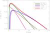 |
Fig. 1 Radial profile of the surface density of our “observation-based” model for the Milky Way’s disk. The curves indicate the surface densities of the thin disk (green), thick disk (brown), H I disk (blue), H2 disk (violet), and the total disk (red). |
2.2. Reproducing the disk mass model with Miyamoto-Nagai disks
2.2.1. The Toomre-Kuzmin disks
As a first step, we make use of the family of disk models of infinitesimal thickness (the razor-thin disks) introduced by Toomre (1963) and Kuzmin (1956), whose densities are written in the form ρ(R,z) = Σ(R) δ(z). The “model 1” of this family, of what we refer to as Toomre-Kuzmin disks (TK-disks), is described by a surface density which is written as ![\begin{equation} \label{eq:disk_TK1} \Sigma_{\mathrm{TK}_{1}}(R)=\frac{a_{\mathrm{TK}_{1}}\,M_{\mathrm{TK}_{1}}}{2\,\pi}\,\frac{1}{\left[R^{2}+a_{\mathrm{TK}_{1}}^{2}\right]^{3/2}}, \end{equation}](/articles/aa/full_html/2016/09/aa27535-15/aa27535-15-eq70.png) (5)where MTK1 is the total disk mass and aTK1 is related to the radial scale length of the disk. The choice of use of TK-disks, in the first step, is because all the information about the disk surface density can be recovered adjusting only two parameters, MTK and aTK. As shown later, the three-dimensional structure of the disks is obtained after “inflating” the TK-disks with the introduction of the parameter b related to the scale height, in the same way as in the original method of Miyamoto & Nagai (1975).
(5)where MTK1 is the total disk mass and aTK1 is related to the radial scale length of the disk. The choice of use of TK-disks, in the first step, is because all the information about the disk surface density can be recovered adjusting only two parameters, MTK and aTK. As shown later, the three-dimensional structure of the disks is obtained after “inflating” the TK-disks with the introduction of the parameter b related to the scale height, in the same way as in the original method of Miyamoto & Nagai (1975).
From Eq. (5), it can be seen that the density ΣTK1 decreases with R-3 at large radii. This is a slower decrease when compared to the observed exponential fall off of the brightness profiles in galaxy disks (Binney & Tremaine 2008). Therefore, a single TK-disk (and the correspondent MN-disk) poorly matches the surface density profile of a radially exponential disk (Smith et al. 2015). This motivated the use of a combination of three MN-disks (related to the “model 1” of TK-disks, Eq. (5)), which was first introduced by Flynn et al. (1996) and since then used for modelling the disk of the Milky Way (Smith et al. 2015, and references therein). In this procedure, each MN-disk has a different scale length a and mass M, with one of the masses with a negative value. The MN-disk with negative mass also has the largest scale length. This feature helps decrease the surface density at large radii (and improve the fit to an exponential disk), but also leads to the undesirable occurrence of regions with negative densities near the mid-plane of the disk and at large radii (Smith et al. 2015).
It is also known that the density ΣTK in Eq. (5) is just the first of a family of possible forms for the potential-density pair that obey the Poisson equation. Toomre (1963) showed that, since the Poisson equation is linear in Φ and ρ, new potential-density pairs can be obtained through the derivation of Φ /an times with respect to a2 (Binney & Tremaine 2008). For example, the densities for “model 2” and “model 3” of the TK-disks are described by ![\begin{equation} \label{eq:disk_TK2} \Sigma_{\mathrm{TK}_{2}}(R)=\frac{3\,a_{\mathrm{TK}_{2}}^{3}\,M_{\mathrm{TK}_{2}}}{2\,\pi}\,\frac{1}{\left[R^{2}+a_{\mathrm{TK}_{2}}^{2}\right]^{5/2}}, \end{equation}](/articles/aa/full_html/2016/09/aa27535-15/aa27535-15-eq86.png) (6)and
(6)and ![\begin{equation} \label{eq:disk_TK3} \Sigma_{\mathrm{TK}_{3}}(R)=\frac{5\,a_{\mathrm{TK}_{3}}^{5}\,M_{\mathrm{TK}_{3}}}{2\,\pi}\,\frac{1}{\left[R^{2}+a_{\mathrm{TK}_{3}}^{2}\right]^{7/2}}, \end{equation}](/articles/aa/full_html/2016/09/aa27535-15/aa27535-15-eq87.png) (7)respectively (Miyamoto & Nagai 1975). One can see that the densities ΣTK2 and ΣTK3 decrease with R-5 and R-7, respectively, at large radii. In this way, a combination of models 2 or 3 of TK-disks could, in principle, not only result in an equally good fit to an exponential disk, but also circumvent the problem of the appearance of negative densities. In our present case, we also need to include a TK-disk with negative mass to the modelling of the central density depression that occurs in the thin stellar disk, the H I and H2 disk subcomponents. The difference here is that the scale length of this component with negative mass does not need to be the largest, thus avoiding the negative densities at large radii. Therefore, for each disk subcomponent (thin, thick, H I, H2), we search for the combination of three TK-disks of each model (1, 2, 3) that better reproduces the radial profile of the surface density of each subcomponent. We take, for example, the case of the thin disk. We search for the set of parameters
(7)respectively (Miyamoto & Nagai 1975). One can see that the densities ΣTK2 and ΣTK3 decrease with R-5 and R-7, respectively, at large radii. In this way, a combination of models 2 or 3 of TK-disks could, in principle, not only result in an equally good fit to an exponential disk, but also circumvent the problem of the appearance of negative densities. In our present case, we also need to include a TK-disk with negative mass to the modelling of the central density depression that occurs in the thin stellar disk, the H I and H2 disk subcomponents. The difference here is that the scale length of this component with negative mass does not need to be the largest, thus avoiding the negative densities at large radii. Therefore, for each disk subcomponent (thin, thick, H I, H2), we search for the combination of three TK-disks of each model (1, 2, 3) that better reproduces the radial profile of the surface density of each subcomponent. We take, for example, the case of the thin disk. We search for the set of parameters  1 of “model 1” of three TK-disks that generates the best fit to the radial distribution of surface density of the thin disk. These three TK-disks result in the total surface density
  . The same procedure is carried out with the three TK-disks in the forms of “model 2” and “model 3”, which result in the total densities
  and
and  , respectively. We quantify ξ2 as the sum over a given radial range of the squares of the residuals between the surface density of the thin disk (obtained from Eq. (1) and parameters from Table 1) and the surface density resulted from the best-fitting combination of the three TK-disks, for each one of the models,
 ![\begin{equation} \label{eq:xi2_dens} \xi_{k,j}^{2}=\frac{1}{N_{R}}\,\sum_{R}^{}\left[\Sigma_{\mathrm{d}_{\,k}}(R)-\Sigma_{\mathrm{TK}_{j}^{\mathrm{tot}}}(R)\right]^{2}, \end{equation}](/articles/aa/full_html/2016/09/aa27535-15/aa27535-15-eq97.png) (8)where k refers to the disk subcomponent (k = thin in the above example) and j denotes the model order of TK-disks; NR is the number of radial bins over which the sum is calculated. The TK-disk model order that results in the lowest value for ξ2 is that which we consider the model that better represents the surface density Σdk of the disk subcomponent. The search for the best sets of parameters
(8)where k refers to the disk subcomponent (k = thin in the above example) and j denotes the model order of TK-disks; NR is the number of radial bins over which the sum is calculated. The TK-disk model order that results in the lowest value for ξ2 is that which we consider the model that better represents the surface density Σdk of the disk subcomponent. The search for the best sets of parameters  corresponding to the best TK-disk models for j was carried by applying the global optimization technique based on the cross-entropy (CE) algorithm for parameters estimation. The CE algorithm (Rubinstein 1997, 1999; Kroese et al. 2006) provides a simple adaptive way of estimating the optimal set of reference parameters in the fitting process. Recent investigations have applied the CE technique to some astrophysical problems, e.g. Caproni et al. (2009), Monteiro et al. (2010), Monteiro & Dias (2011), Martins et al. (2014), Dias et al. (2014), Caetano et al. (2015), among others. Since we also employ the CE method on other occasions throughout this paper, in the next subsection we give a brief description of the main steps of the algorithm. Table 2 summarizes the model of three TK-disks found to better reproduce the surface density of each one of the disk subcomponents and the corresponding ξ2 (Eq. (8)) minimized within the CE algorithm.
Models of 3 TK-disks that provide the best match to the surface density of each disk subcomponent.
2.2.2. The cross-entropy algorithm
For a detailed presentation and description of the CE method, see the papers by Monteiro et al. (2010), and Dias et al. (2014). Here, we give a brief overview of the method and how it works.
Supposing we have a set of data D with individual points d1, d2, ..., dND and we wish to study it in terms of an analytical model Θ with a vector of parameters θ1, θ2, ..., θNp. The main goal of the CE continuous multiextremal optimization method is to find a set of parameters  for which the model provides the best description of the data, based on some statistical criterion. This is performed by randomly generating N independent sets of model parameters
  , where
  , under some chosen distribution, and the subsequent minimization of an objective function S(X) is used to transmit the quality of the fit during the run process. As the method converges to the “theoretical” exact solution, then S → 0, which means
  .
.
The CE method performs an iterative statistical coverage of the parameter space, where the following is carried out in each iteration (Monteiro et al. 2010):
-
(i)
random generation of the initial parameter sample, respectingsome underlying distributions and pre-defined criteria;
-
(ii)
selection of the best candidates based on some mathematical criterion, which will compose the elite sample array – samples with the lowest values for the objective function S(X);
-
(iii)
random generation of updated parameter samples from the previous best candidates, i.e. the elite sample, to be evaluated in the next iteration;
-
(iv)
optimization process repeats steps (ii) and (iii) until a pre-specified stopping criterion is fulfilled.
In all the implementations of the CE algorithm carried out in this work, we followed the general step by step presented in Sect. 2.2 of Monteiro et al. (2010). The tuning parameters used in the run processes were N = 3 × 10³ sets of trial model parameters per iteration; a maximum number of 100 iterations; Nelite = 100, which is the number of sets of trial parameters that return the best solutions (the lowest values for the objective function) at a given iteration and that will be used to estimate the distribution parameters for the next iteration. For the smoothing parameters that reduce the convergence speed of the algorithm, preventing it from finding a non-global minimum solution, we have used α = 0.9, α′ = 0.7, and q = 7. For more details about these parameters and how they are implemented in the algorithm, see Monteiro et al. (2010).
2.2.3. The Miyamoto-Nagai disks – following the approach developed by Smith et al. (2015)
Once the models of TK-disks have been found, the next step is to “inflate” them vertically to find the correspondent MN-disks. As firstly performed by Miyamoto & Nagai (1975), this is carried out by replacing the term (a + | z |) in the potential function, which is associated with the density of a given model of TK-disk, with the term ![\hbox{$\left[a+\sqrt{z^{2}+b^{2}}\right]$}](/articles/aa/full_html/2016/09/aa27535-15/aa27535-15-eq124.png) , where b expresses the vertical scale height of the disk. In this way, corresponding to the three models of TK-disks expressed by Eqs. (5)–(7), we have the following three-dimensional density functions that compose the first three models of MN-disks:
, where b expresses the vertical scale height of the disk. In this way, corresponding to the three models of TK-disks expressed by Eqs. (5)–(7), we have the following three-dimensional density functions that compose the first three models of MN-disks: ![\begin{eqnarray} \label{eq:rho_MN1} \rho_{\mathrm{MN}_{1}}(R,z)&=&\left(\frac{b^{2}M}{4\pi}\right)\frac{\left[a R^{2}+\left(a+3\zeta\right)\left(a+\zeta\right)^{2}\right]}{\zeta^{3}\left[R^{2}+\left(a+\zeta\right)^{2}\right]^{5/2}}, \\ \label{eq:rho_MN2} \rho_{\mathrm{MN}_{2}}(R,z)&=\left(\frac{b^{2}M}{4\pi}\right)\frac{3\,\left(a+\zeta\right)}{\zeta^{3}\left[R^{2}+\left(a+\zeta\right)^{2}\right]^{7/2}}\left[R^{2}\left(\zeta^{2}-a\zeta+a^{2}\right)\right.\notag \\ & &\quad +\left.\left(a+\zeta\right)^{2}\left(\zeta^{2}+4a\zeta+a^{2}\right)\right], \\ \label{eq:rho_MN3} \rho_{\mathrm{MN}_{3}}(R,z)&=\left(\frac{b^{2}M}{4\pi}\right)\frac{1}{\zeta^{3}\left[R^{2}+(a+\zeta)^{2}\right]^{9/2}}\,\left[3R^{4}\zeta^{3}\right.\nonumber\\ &&\quad+R^{2}(a+\zeta)^{2}\left(6\zeta^{3}+15a\zeta^{2}-10a^{2}\zeta+5a^{3}\right)\nonumber\\ &&\quad+\left.(a+\zeta)^{4}\left(3\zeta^{3}+15a\zeta^{2}+25a^{2}\zeta+5a^{3}\right)\right], \end{eqnarray}](/articles/aa/full_html/2016/09/aa27535-15/aa27535-15-eq125.png) where
where  . In the above expressions, for the sake of good readability, we avoided the excessive use of subscripts in the parameters M, a, b, and ζ that could distinguish between each one of the models. Here, we make it clear that for each disk subcomponent modelled with a combination of three TK-disks of a given model, we use the corresponding combination of three MN-disks of the equivalent model.
Parameters of the three MN-disk combinations for modelling each subcomponent of the Galactic disk.
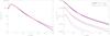 |
Fig. 2 Left-hand panel: radial distribution of the surface mass density of the Galactic disk model; the “observation-based” disk model (blue curve) and the resultant from the sum of all the 3 MN-disk combinations fitted to each disk subcomponent (red curve). Right-hand panel: vertical profile of the volume density of the Galactic disk model as a function of the height z from the mid-plane and at three different arbitrary radii: R = 2 kpc (solid lines); R = 8 kpc (R0) (dashed lines); and R = 15 kpc (dotted lines). The blue curves are also related to the “observation-based” disk model and the red curves to the total 3 MN-disk combinations. |
The task now is to find the best values for the parameter b that reproduce the vertical density distribution of each subcomponent of the Galactic disk. For this purpose, we follow the approach recently developed by Smith et al. (2015). In that work, the authors create a procedure for modelling simple radially exponential disks from the combination of three MN-disks of “model 1”, allowing the construction of disks of any mass, scale length, and for an ample range of thicknesses, from infinitely thin disks to approximately spherical systems. The basic idea of the method is as follows: Starting from the model composed of the three TK-disks (for which b = 0) that better match the radial profile of the disk surface density, one chooses the corresponding model composed of three MN-disks with a small value for the b parameter (with the aim of remaining near the solution for the infinitesimal thickness disk), and whose parameters M and a of the MN-disks deviate from small amounts with respect to those of the TK-disks. With the continuous variation of b in small steps, the parameters M and a are searched for at intervals close to the solution found in the previous step, ensuring a smooth variation of both M and a with the variation of the disk thickness b. In fact, Smith et al. (2015) analyse the variation of the ratios M/Md and a/Rd as a function of the variation of the ratio b/Rd, where Md is the mass and Rd is the radial scale length of the exponential disk to be modelled. Therefore, for each small variation of the ratio b/Rd, one searches for the parameters M and a of the three MN-disks whose integral of the density ρ(z) in the vertical direction better reproduces the radial profile of the disk surface density Σ(R).
To relate the scale height b of the MN-disks with the scale height hz of the vertically exponential disk, Smith et al. (2015) follow an approach that is analogous to that described above. In this case, the authors first sum up the fractional differences between the density of the three MN-disks combination and the exponential density, measured vertically from the mid-plane up to z = 5b. These authors vary the ratio b/Rd to minimize the sum, and then find the best match to the exponential distribution.
In this section, we only present the values of the parameters [M,a,b] calculated for each combination of three MN-disks that fit each disk subcomponent with their fixed values for [Md,Rdexp,hz] listed in Table 1. However, in Appendix A, we also present the variations of the ratios M/Md and a/Rdexp, as a function of b/Rdexp, and the relations between b/Rdexp and hz/Rdexp for each disk subcomponent, calculated in the same way as in Smith et al. (2015). Therefore, disks of any mass Md and scales Rdexp and hz can be built up using those relations, but remembering here that they are suited for models of disks with central density depressions. Since the majority of our disk subcomponents are no longer modelled by a single radially exponential law (cf. Eqs. (1) and (3)), coupled with the fact that we also use models of higher order (2 and 3) than model 1 of MN-disks, our calculated relations between the aforementioned parameters are somewhat different from those presented in Smith et al. (2015). But with equivalent utility, the relations in Appendix A allow the construction of models for disks with masses and sizes that are different from those modelled in this work.
In our search for the best values of the parameters [M,a,b] of the MN-disks, we also employed the CE technique described in the previous subsection, but now look for the minimization of the sum of the squares of the residuals between the surface density of the disk subcomponent and the vertically integrated volume density of the three MN-disk combinations ![\begin{equation} % \xi_{k,j}^{'2}=\frac{1}{N_{R}}\,\sum_{R}^{}\left[\Sigma_{\mathrm{d}_{\,k}}(R)-\int_z\rho_{\mathrm{MN}_{j}^{\mathrm{tot}}}(R,z)\,\mathrm{d}z\right]^{2}, \end{equation}](/articles/aa/full_html/2016/09/aa27535-15/aa27535-15-eq151.png) (12)for the relations of M/Md and a/Rdexp with b/Rdexp, and the minimization of the sum of the squares of the fractional differences between the volume densities of the three MN-disk combinations and the disk subcomponent over a given vertical range and at R = R0
(12)for the relations of M/Md and a/Rdexp with b/Rdexp, and the minimization of the sum of the squares of the fractional differences between the volume densities of the three MN-disk combinations and the disk subcomponent over a given vertical range and at R = R0![\begin{equation} % \xi_{k,j}^{''2}=\frac{1}{N_{z}}\,\sum_{z}^{}\left[\frac{\rho_{\mathrm{d}_{\,k}}(z)-\rho_{\mathrm{MN}_{j}^{\mathrm{tot}}}(z)}{\rho_{\mathrm{d}_{\,k}}(z)}\right]^{2}, \end{equation}](/articles/aa/full_html/2016/09/aa27535-15/aa27535-15-eq152.png) (13)for the relations between b/Rdexp and hz/Rdexp.
(13)for the relations between b/Rdexp and hz/Rdexp.
We return to the case of the thin stellar disk for exemplification. With the ratio hz/Rdexp calculated from the values listed in Table 1 for the thin disk, and putting it into Eq. (A.1) with the coefficients for the thin disk given in Table A.1, both from Appendix A, one finds the corresponding value for the ratio b/Rdexp. Substituting this last value into Eq. (A.2) with the coefficients given in Table A.2, also from Appendix A, one obtains the values of the parameters Mi and ai for the combination of three MN-disks of model 3 (Eq. (11)), which matches the density distribution ρd★, thin of the thin stellar disk better. We emphasize here that a single scale height b is used for all the three MN-disks of the combination, as originally carried out by Flynn et al. (1996) and followed by Smith et al. (2015). The entire procedure described above, which was illustrated with the thin disk, is repeated with the other subcomponents (thick disk, H I, and H2 disks) using their corresponding equations and tables in Appendix A. Table 3 lists the values of the parameters [M,a,b] of each combination of three MN-disks that fit each disk subcomponent and the correspondent models of MN-disks that had been previously found with modelling of TK-disks.
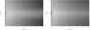 |
Fig. 3 Contours of iso-densities log ρ for the disk models built in the present work. Left-hand panel: the “observation-based” disk model; right-hand panel: the sum of all three MN-disk combinations fitted to each disk subcomponent. The values of the contours lie in the range log ρ = [−6; +1], with ρ in M⊙ pc-3. |
Figure 2 shows, in the left-hand panel, the radial profile of the surface mass density for the “observation-based” disk model (blue curve) and the total surface density resultant from all the three MN-disk combinations fitted to each disk subcomponent (red curve). A good agreement is seen between these two curves, which denotes the great effectiveness of the method. The fractional differences between these surface density distributions are <10% at 1 kpc ≲ R ≲ 21.5 kpc, reaching 50% at R ~ 26 kpc and 100% at R ~ 29 kpc, where the absolute values of the densities become lower than ~0.5M⊙ pc-2. These features show the tendency of the MN-disks to return larger densities at large radii. The local disk surface density returned by the MN-disk fit models is Σ0d = 59.4M⊙ pc-2, which can be considered close to the prior value of 57.2 M⊙ pc-2 of the “observation-based” disk model, if we take the uncertainty of ± 4.9M⊙ pc-2 over this quantity as estimated by Read (2014). The local surface density integrated within 1.1 kpc of the disk mid-plane returned by the MN-disk fit models is Σ0d1.1 kpc = 57.0M⊙ pc-2, in agreement with the values reported by Bienaymé et al. (2006). On the right-hand panel of Fig. 2, we show the distribution of the volume density as a function of the height z from the disk mid-plane, taken at three arbitrary radii: R = 2 kpc (solid line), R = 8 kpc (dashed line), and R = 15 kpc (dotted line). The blue and red curves also correspond to the density distributions of the “observation-based” disk model and the MN-disk fit models, respectively. The fractional differences between the volume density distributions are lesser than 25% for | z | ≲ 2.3 kpc at R = 2 kpc, for | z | ≲ 1 kpc at R = 8 kpc, and for | z | ≲ 0.35 kpc at R = 15 kpc, reaching values that are greater than 25% beyond these heights. These features denote the systematic trend of the MN-disks to return higher densities at greater distances from the disk plane, while at relatively small z the density distributions show roughly good matches at radii up to at least R ~ 22 kpc. As pointed out by Smith et al. (2015), it is impossible for the three MN-disk models to perfectly reproduce the vertically exponential density profile or even the sech2(z) type profile, since they are mathematically distinct. The same can be stated about the vertical Gaussian profile adopted for the H I and H2 disks in the present work; at heights lower than 1 kpc the three MN-disks start presenting great deviations from the Gaussian profile. This can be noticed by analysing the distributions of ρ(z) calculated at R = 15 kpc (dotted lines in the right-hand panel of Fig. 2), where the density of the H I disk overtakes those of the other disk subcomponents (cf. Fig. 1).
Figure 3 shows the contours of iso-densities in the form log ρ (ρ in M⊙ pc-3) in the meridional plane of the Galaxy: for the “observation-based” disk model (left-hand panel) and for the total three MN-disk combination fit models (right-hand panel).
2.3. The gravitational potential of the disk
The gravitational potential expressions related through Poisson equation to the densities of the Miyamoto-Nagai disk models, given by Eqs. (9)–(11), are written as “model 1”, “model 2”, and “model 3”, respectively, in the form ![\begin{eqnarray} \label{eq:Phi_MN1} \Phi_{\mathrm{MN}_{1}}(R,z)&=&\frac{-GM}{\left[R^{2}+\left(a+\zeta \right)^{2}\right]^{1/2}}, \\ \label{eq:Phi_MN2} \Phi_{\mathrm{MN}_{2}}(R,z)&=&\frac{-GM}{\left[R^{2}+\left(a+\zeta \right)^{2}\right]^{1/2}}\left[1+\frac{a(a+\zeta)}{R^{2}+(a+\zeta)^{2}} \right], \\ \label{eq:Phi_MN3} \Phi_{\mathrm{MN}_{3}}(R,z)&=&\frac{-GM}{\left[R^{2}+\left(a+\zeta \right)^{2}\right]^{1/2}}\left\{1+\frac{a(a+\zeta)}{R^{2}+(a+\zeta)^{2}}\right.\notag\\ & \quad -\left.\frac{1}{3}\frac{a^{2}\left[R^{2}-2(a+\zeta)^{2}\right]}{\left[R^{2}+(a+\zeta)^{2}\right]^{2}}\right\}, \end{eqnarray}](/articles/aa/full_html/2016/09/aa27535-15/aa27535-15-eq173.png) where again . Therefore, the gravitational potential of the thin stellar disk Φd thin is modelled with three components of the potential ΦMN3 (Eq. (16)), whose parameters Mi, ai, and b (i = 1, 2, 3) are given in the first row of Table 3. Equivalently, the thick stellar disk potential Φd thick is modelled with three components of the potential ΦMN1 (Eq. (14)), the H I disk potential Φd HI is modelled with three components of ΦMN2 (Eq. (15)), and the H2 disk potential Φd H2 with three components of the potential ΦMN3 (Eq. (16)); the parameters Mi, ai, and b for these disks are given in the second, third, and fourth rows, respectively, of Table 3. The total gravitational potential of the disk Φd is then given by the sum of all the combinations of three MN-disks that fit each Galactic disk subcomponent,
where again . Therefore, the gravitational potential of the thin stellar disk Φd thin is modelled with three components of the potential ΦMN3 (Eq. (16)), whose parameters Mi, ai, and b (i = 1, 2, 3) are given in the first row of Table 3. Equivalently, the thick stellar disk potential Φd thick is modelled with three components of the potential ΦMN1 (Eq. (14)), the H I disk potential Φd HI is modelled with three components of ΦMN2 (Eq. (15)), and the H2 disk potential Φd H2 with three components of the potential ΦMN3 (Eq. (16)); the parameters Mi, ai, and b for these disks are given in the second, third, and fourth rows, respectively, of Table 3. The total gravitational potential of the disk Φd is then given by the sum of all the combinations of three MN-disks that fit each Galactic disk subcomponent,  (17)Figure 4 shows the contours of equipotential curves in the plane R − z for the gravitational potential of the disk Φd, which is expressed in Eq. (17).
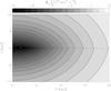 |
Fig. 4 Contours of equipotentials in the Galactic meridional plane for the gravitational potential resulting from the disk model composed of combinations of MN-disks, as described in Sect. 2.2.3. The contours of Φd are given in 104 km2 s-2, as indicated in the colourbar. |
3. Galactic models
3.1. Bulge and dark halo components
For the mass density distribution in the spheroidal component of the Galaxy, here assumed as composed of the central bulge and the stellar halo as a smooth extension of the bulge itself, we adopt the profile proposed by Hernquist (1990), which reproduces the r1/4de Vaucouleurs (1977) surface brightness law over a large range of galactic radius, 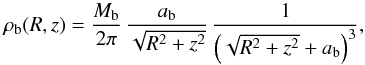 (18)where Mb is the total mass and ab is the scale radius of the bulge. The gravitational potential associated with the density distribution in Eq. (18) was shown by Hernquist (1990) to be in the form
 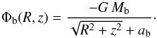 (19)In the PJL star counts model, the bulge is modelled as an oblate spheroid, which is described by a modified Hernquist profile with three free parameters: the oblateness parameter κ, the spheroid-to-disk local stellar density ratio for normalization of the density profile, and the spheroid scale radius aH = 0.4 ± 0.1 kpc. Considering the local stellar density of our “observation-based” disk model, the mass of the spheroid of the PJL model inside R = 3 kpc (a radius that encompasses ~90% of the total spheroid mass) results in Msph(R< 3 kpc) ≈ 2.2 × 10¹⁰M⊙. We use this information to constrain the initial ranges of the parameters Mb and ab of our bulge models to search for their best values in the fitting procedure described in Sect. 5. We adopt the initial guess interval Mb = 2.4–2.8 × 10¹⁰M⊙ for the bulge mass; we use ab = 0.3–0.5 kpc for the scale radius. These intervals comprise masses inside R = 3 kpc for our bulge models with possible values in the range 1.8–2.3 × 10¹⁰M⊙.
The fact that the observed rotation curve, which is adopted to constrain the Galactic models, is nearly flat in the interval R0 ≲ R ≲ 2R0 (see Sect. 4), and besides the fact that in our models (see Sect. 6) the sole disk plus bulge density distributions are not capable of giving such support to the rotation curve at these radii, leads us to take into consideration the contribution of an extra mass component to which we refer by the often-used term “dark halo”. Since there is still some tension in the explanations for the behaviour of the rotation curves at large radii of some external spiral galaxies, as for the Milky Way, we do not reflect on the reality of such a dark halo component nor its material content, although the dark halo contributes an extra term of mass in our Galactic models. For this reason, we do not go deeper in the modelling of such a component and take simple forms for its density and potential functions.
We model the dark halo component with a logarithmic potential of the form (e.g. Binney & Tremaine 2008) 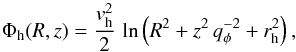 (20)where rh is the core radius; vh is the circular velocity at large r, i.e. relative to the core radius; and qφ is the axis ratio of the equipotentials. For simplicity, we consider a spherical dark halo, for which qφ = 1. The density distribution corresponding to the potential Φh is given by (for qφ = 1)
 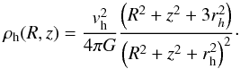 (21)This profile yields a flat rotation curve at large radii. However, as we make clear in the following sections, we are interested in a description of the Galactic potential that can be suitable for the study of stellar orbits that do not reach great extensions of the outer disk, so the real behaviour of the rotation curve of the Galaxy at very large radii is not of concern in the present study.
The values of the parameters Mb and ab that describe the bulge component, rh, and vh for the dark halo are found after fitting the contributions of such components to the Galactic rotation curve as well as to other observational constraints as described in Sect. 4.
3.2. The disk component
The model constructed for the mass distribution in the disk of the Galaxy, and its associated gravitational potential, is described in detail in the subsections of Sect. 2. In general, the overall disk is modelled by a superposition of distinct models of Miyamoto-Nagai disks; these models are comprised of combinations of three MN-disks for each one of the four subcomponents: thin, thick, H I, and H2 disks yielding 12 MN-disks in total. Each MN-disk has three free parameters (M, a, b), but since each combination of three MN-disks is modelled with a single value for b (see Sect. 2.2.3), we have a total of 28 parameters for the construction of the disk (all of these parameters are given in Table 3).
In the present work, in contrast to other studies, the values of the structural parameters of the disk (here represented by the length scales a and b of the MN-disks) are not constrained by the kinematic information from the rotation curve of the Galaxy. Here, we opt to constrain such parameters based only on the information brought by the star-counts model of PJL and the observed distribution of the gaseous component in the disk. However, some of the disk scale parameters in the Galactic model of PJL possess considerable uncertainties, as for instance the radial length of the central hole of the thin disk  kpc, which the kinematic data would help to reduce. Although this can represent a drawback of our approach, in Sect. 5 we give an estimate of the uncertainties on the parameters a and b of the MN-disks based on the uncertainties on the scale parameters of the “observation-based” disk model. Our reason for leaving the scale parameters fixed at the values from Table 3 is justified owing to the way the MN-disks were constructed; the scale lengths a were found as functions of the scale heights b, and they should preserve the relationships during the fitting of the kinematic data. However, a proper fitting of the kinematic constraints should vary these scale lengths in an independent way to probe the correlations among the parameters. Moreover, it is well known in the literature that the kinematic data commonly used for the model fittings do not provide strong constraints on the vertical distribution of the Galaxy’s mass (e.g. Dehnen & Binney 1998; McMillan 2011). Therefore, different sets of disk scale heights would be found able to reproduce the kinematic data equally well. Another problematic issue in varying the scales a and b of all the MN-disks in the fitting of the models, taking into account the uncertainties on the values of Rd, Rch, and hz of all the disk subcomponents, is the long computing time involved in the whole process. We recognize this disadvantageous point of our approach in fitting MN-disks to the observed disk; other studies in the literature that do not make use of this approximation are able to vary the scale parameters of their disk potential models in a more straightforward way (e.g. McMillan 2011; Piffl et al. 2014a).
The total mass of the disk, otherwise, is left to be constrained not only by the rotation curve that provides information on the dynamical mass of the Galaxy, but also by prior information on the local disk surface density in visible matter. Therefore, for the fitting of the disk model to the observational constraints described in Sect. 4, we take the values of the scale lengths ai and scale heights b of the MN-disks as fixed and equal to those given in Table 3. The total mass of the disk is adjusted by introducing the parameter fmass, a scale factor by which the disk total mass is then multiplied. Once the best value for fmass is found, then the masses Mi of all the MN-disks in Table 3 have to be multiplied by this factor. In this way, in the fitting process of the disk model based on the dynamical constraints, only the disk total mass is treated as a free parameter. Although the individual masses Mi of the MN-disks have already been found after the construction of the disk mass model in Sect. 2, in the next step we use their single values in Table 3 as first guesses for the optimal fit values to the dynamical constraints, but keeping their relative contributions to the disk total mass unaltered since all of them are rescaled by the same factor fmass.
3.3. An alternative model: a disk with a ring density structure near the solar orbit radius
There are reasons to believe that the Galactic disk presents a local minimum of density associated with the co-rotation resonance radius of the Galactic spiral structure. Such a minimum density would be present in both the stellar and gaseous disks components. A structure like this has been observed in the hydrogen distribution of the disk, as discussed later in this section. A minimum in the density of Cepheids is seen at the same radius (BLJ, see their Fig. 14). However, as they are relatively young, the Cepheids possibly trace the gas distribution and therefore the recent past of star formation. There are theoretical argumentation and simulations given in BLJ that predict that the co-rotation resonance scatters the stars out from that radius, situated close to the solar radius, and produces a minimum in the stellar density. However, there is no direct strong evidence from photometric studies of the disk for such a ring of minimum density of stars. For this reason, our proposed ring density structure is still a speculative one, which we attempt to test in this work.
In Zhang (1996), based on N-body simulation results of a spiral galaxy evolution and also on theoretical predictions about secular processes of energy and angular momentum transfer between stars and the spiral density wave, the author showed that a local minimum in the stellar density of the disk is formed, centred at the co-rotation radius. BLJ performed numerical integrations of test-particle orbits with a representative model for the potential due to the axisymmetric density distribution in the Galactic disk and models for the gravitational perturbation due to the spiral arms. The authors verified that a minimum of stellar density with relative amplitude ~30%–40% of the background density is formed at the co-rotation radius in a time interval ~3 billion years of the evolution of the system. Lépine et al. (2001), based on a simulation of gas-cloud dynamics in the spiral gravitational field model of the Galaxy, also verified a gap in the ISM distribution at the co-rotation radius. The authors compared their results (cf. their Fig. 4) with the observed H I radial distribution presented by Burton (1976, see his Fig. 6) and found close similarities between them. Such results are compatible with evidence for a ring that is void of gas, as observed by Amôres et al. (2009) as gaps in the H I density distributed in a ring-like structure with radius slightly outside the solar circle. Recent studies on the three-dimensional distribution of the neutral and molecular hydrogen in the Galactic disk by Nakanishi & Sofue (2016) and Sofue & Nakanishi (2016) also corroborate the existence of the minimum gas density slightly beyond the solar Galactic radius. Since the co-rotation resonance is observed to be at a slightly larger but very close radius to the solar orbit radius (e.g. Dias & Lépine 2005), then the solar orbit would be placed close to the minimum of the disk surface density.
Lépine et al. (2001) associated the minimum in the stellar and gas density distributions with a local dip in the observed rotation curve of the Galaxy at R ~ 9 kpc. A common association between these two features was also modelled by Sofue et al. (2009). In the simulation results of BLJ, the minimum density at co-rotation is followed by a local maximum density at a slightly larger radius. BLJ modelled such a density feature as a wavy ring superposed on the surface density profile of the disk following Sofue et al. (2009).
Since we still have no clue of how the three-dimensional distribution of this density feature might appear, we make the simplest assumption that it would be mainly detected in the density distribution very near the mid-plane of the disk. Hence we can take the zero-thickness disk approximation for the surface density of the ring. We propose a tentative analytical function for the gravitational potential associated with the ring density (local minimum followed by a maximum density), which is written in the form ![\begin{eqnarray} \label{eq:pot_ring} &&\Phi_{\rm ring}(R,z)=\varphi_{R}(R)\cdot\varphi_{z}(z),\, \quad \mathrm{where} \nonumber\\ \nonumber\\ &&\varphi_{R}(R)=-A_{\rm ring}\,\mathrm{sech}\left[\ln\left(\frac{R}{R_{\rm ring}}\right)^{\beta_{\rm ring}}\right]\,\tanh\left[\ln\left(\frac{R}{R_{\rm ring}}\right)^{\beta_{\rm ring}}\right] \\ &&\mathrm{and}\nonumber \\ &&\varphi_{z}(z)=\mathrm{sech}\left(\frac{z}{h_{z_{\rm ring}}}\right),\nonumber \end{eqnarray}](/articles/aa/full_html/2016/09/aa27535-15/aa27535-15-eq213.png) (22)where Aring is the amplitude of the potential related to the amplitude of the minimum and maximum densities of the ring, given in units of km2 s-2; βring is a parameter related to the ring width; Rring is the ring node radius, where the inflection point between the minimum and maximum density features sits; and hzring is the scale height of the ring potential. Solving the Poisson equation for the ring potential ∇2Φring = 4πGΣringδz (within the zero-thickness assumption), we can find the corresponding expression for the ring surface density Σring.
(22)where Aring is the amplitude of the potential related to the amplitude of the minimum and maximum densities of the ring, given in units of km2 s-2; βring is a parameter related to the ring width; Rring is the ring node radius, where the inflection point between the minimum and maximum density features sits; and hzring is the scale height of the ring potential. Solving the Poisson equation for the ring potential ∇2Φring = 4πGΣringδz (within the zero-thickness assumption), we can find the corresponding expression for the ring surface density Σring.
In the model that includes the ring structure, the surface density Σring is added to the disk surface density Σd, but since the ring is modelled by a minimum followed by a maximum density of similar amplitudes, which makes the net ring mass Mring ~ 0, the disk total mass is then kept approximately unaltered. With the ring density structure, the Galactic models are adjusted with the inclusion of the ring free parameters: Aring, βring, and Rring; the scale height hzring is chosen to be fixed at a predetermined value.
The inclusion of the ring density feature in the Galactic models is translated in a rescaling of the disk total mass towards larger values when compared to the disk models without the ring. This result is better discussed in Sect. 6.3.
4. Observational constraints
In this section we present the groups of observational data used to constrain the free parameters of the Galactic models introduced in Sect. 3. These groups basically comprise kinematic data from the rotation curve of the Galaxy, with tangent velocities at radii R<R0 and rotation velocities at R>R0, the local angular rotation velocity Ω0, and values for the estimated total local disk mass-surface density Σ0d already discussed in Sect. 2, as well as the surface density integrated within 1.1 kpc of the disk mid-plane. In the following, we discuss each group of constraints.
4.1. The local angular rotation velocity and the solar kinematics
In this work, we take the Galactocentric distance of the Sun R0 from the statistical analysis performed by Malkin (2013) on 53 R0 measurements published in the literature over the last 20 yrs, whose average value, for practical purposes, is recommended by the author as written as  For the peculiar velocity of the Sun v⊙ relative to the local standard of rest (LSR), we take the re-evaluation proposed by Schönrich et al. (2010, hereafter SBD),
  where we use a left-handed system for (U, V, W), in which U is positive towards the Galactic anti-centre, V is positive in the direction of Galactic rotation, and W is positive towards the direction of the North Galactic Pole; (u⊙,v⊙,w⊙) are the Sun’s velocity components in such system. The above-quoted uncertainties are the systematic ones, since these dominate the total uncertainties as estimated by SBD.
To constrain the angular velocity of the Sun Ω⊙, we consider the direct measurement of Sgr A∗ proper motion along the Galactic plane carried out by Reid & Brunthaler (2004), whose value is μSgr A∗ = 6.379 ± 0.024 mas yr-1. Thus we have Ω⊙ = μSgr A∗ = 30.24 ± 0.11 km s-1 kpc-1. This last equality comes from the assumption that Sgr A∗ is at rest at the Galactic centre, so its apparent proper motion can be thought to be solely due to the sum of the Galactic rotation at the LSR and the solar peculiar motion with respect to the LSR in the same direction, i.e. Ω⊙ ≡ Ω0 + v⊙/R0 (e.g. Honma et al. 2012). We then have  (23)for the local angular rotation velocity Ω0. With the above-quoted values for Ω⊙, v⊙, and R0, one obtains Ω0 = 28.7 km s-1 kpc-1. The uncertainty on Ω0 is calculated as
  , which returns the value σΩ0 = 0.4 km s-1 kpc-1; to the uncertainty σv⊙ of 2 km s-1 given by SBD, we added 1 km s-1 to allow for a possible peculiar motion of Sgr A∗ at the Galactic centre (McMillan & Binney 2010). The corresponding rotation velocity at the LSR, V0 = Ω0R0, assumes the value V0 = 230 ± 8 km s-1.
4.2. The rotation curve
4.2.1. Tangent velocities
The tangent (or terminal) velocity Vterm is usually assumed as the maximum velocity of the ISM gas along a given line of sight at Galactic coordinates b = 0° and −90° ≤ l ≤ 90°, which can be related to the circular velocity Vc(R) at the tangent point R = R0sinl (or sub-central point), considering a circularly rotating gas. For the tangent velocity data, we use the CO-line data inside the solar circle from Table 2 of Clemens (1985)2, which cover longitudes in the first Galactic quadrant. We also use the H I tangent point data from Table 2 of Fich et al. (1989), which cover both the first and fourth Galactic quadrants. We converted the LSR tangent velocities of these compiled data to heliocentric velocities and then back to LSR tangent velocities using the components of the peculiar solar motion adopted in this work. Then the Galactocentric distances R = R0sinl and the rotation velocities Vrot = Vterm + V0sinl were calculated using the Galactic constants adopted in this work (R0, V0) = (8 kpc, 230 km s-1). We propagated the uncertainties on both R0 and V0 to the uncertainties on R and Vrot (σR and σVrot), respectively.
It has often been argued that the central region of the Galaxy is strongly affected by non-axisymmetric structures such as the bar, which can induce non-circular motions of the ISM. The true Galactic rotation curve would then be distorted by the measurement of non-uniform azimuthal velocities, making the tangent-point method inappropriate at these regions. Recently, Chemin et al. (2015) attempted to quantify the asymmetries in the Galactic rotation curve derived by the tangent-point method. Figure 3 of Chemin et al. (2015) shows that the largest discrepancies between the first and fourth quadrant rotation curves are in the interval 1 ≲ R ≲ 2 kpc. Perhaps the most delicate feature in the Milky Way inner rotation curve, as derived from the tangent-point method, is the velocity peak at R ~ 300 pc. Based on a numerical simulation of a disk galaxy similar to the Milky Way, Chemin et al. (2015) concluded that the tangent velocities lead to an inner velocity profile with a peak that is not present in the true rotation curve, when the bar major axis is viewed with angles <45° with respect to the direction of the galaxy’s centre. However, we argue that the interpretation of this inner peak as due to the contribution of the bulge can still be defensible: at R ~ 300 pc, a centrally concentrated bulge might dominate the rotation curve, while the bar, as a more extended structure, might influence the rotation curve at radii larger than that.
Also based on the simulated galaxy, Chemin et al. (2015) show that the resulting velocity profile strongly deviates from the true rotation curve in the region R< 4 kpc; the tangent-point method in the inner regions systematically select high-velocity gas along the bar and spiral arms, or low-velocity gas in the less dense media. The authors state that the observed rotation curve of the Milky Way derived by the tangent-point method is expected to be close to the true rotation curve only for radii 4 ≲ R ≤ 8 kpc. The unreliable rotation curve at 2 ≲ R ≲ 4 kpc in the Chemin et al. simulation is attributed to effects associated with the co-rotation of the bar, which have a pattern speed of the order of 59 km s-1 kpc-1 in their model. Other authors have obtained lower values for the bar pattern speed, for example 30–40 km s-1 kpc-1 (Rodriguez-Fernandez & Combes 2008) or 33 km s-1 kpc-1 (Li et al. 2016). These lower patterns would put the bar co-rotation at radii larger than 4 kpc. The tangent-point data from Fich et al. (1989) show a velocity difference on the two sides of the Galactic centre, which is of the order of 12 km s-1 on average, in the range R = 2–4 kpc. We think that this amplitude of asymmetry, contrary to that observed in the region 1 <R< 2 kpc, does not influence our models. Given the considerations presented above, we decided to restrict the tangent velocity data to | sinl | ≥ 0.3 (e.g. Dehnen & Binney 1998), which in our case is equivalent to Galactic radii R ≥ 2.4 kpc. We end up with a data set that totalizes 280 rotation velocity measurements in the inner solar circle region (2.4 ≤ R ≤ 8.0 kpc).
4.2.2. Maser sources data
From very long baseline interferometry techniques, several maser sources associated with high-mass star-forming regions (HMSFRs) have been studied and their positions, parallaxes, and proper motions have been measured with high accuracy. Complementing these data with heliocentric radial velocities from Doppler shifts, we are able to access the full three-dimensional location of each source in the Galaxy as well as their full space motion relative to the Sun. Since it is believed that the maser sources do not present large peculiar motions, we can use their velocity components in the direction of Galactic rotation as a proxy for the rotation curve of the Galaxy (Irrgang et al. 2013), taking for this the value of v⊙ estimated by SBD. The data for HMSFRs with maser emission were obtained from Table 1 of Reid et al. (2014), where the authors list parallaxes, proper motions, and LSR radial velocities of 103 regions measured with Very Long Baseline Interferometry (VLBI) techniques from different surveys and projects (the Bar and Spiral Structure Legacy (BeSSeL) Survey3 and the Japanese VLBI Exploration of Radio Astrometry (VERA)4). We converted the tabulated LSR radial velocities to heliocentric radial velocities by adding back the components of the standard solar motion (Reid et al. 2009). With the coordinates, parallaxes, proper motions, heliocentric radial velocities, and their respective errors, we calculated the heliocentric U, V, W velocities and uncertainties σU, σV, and σW for each source, following the formalism described by Johnson & Soderblom (1987). Correcting for the SBD solar peculiar motion and for the LSR circular velocity V0, we calculated the Galactocentric component Vφ of the space velocity of each maser source in the direction of Galactic rotation. The uncertainties on Vφ and σVφ were obtained by propagation from the uncertainties on the parallaxes, proper motions, heliocentric radial velocities, and the uncertainties of the solar motion. The rotation velocities and uncertainties were then defined by Vrot = Vφ and σVrot = σVφ. The Galactic radii were obtained directly from the positions and parallaxes of the sources as well as their uncertainties. The distribution of Galactic radii comprises regions both inside and outside the solar circle. We discarded the sources with radii R< 4 kpc because most of them present values of Vφ with large deviations from the rotation curve that are traced by the tangent velocity data at these radii; a similar selection criterion was used by Reid et al. (2014). This selection reduces the number of maser sources used to probe the rotation curve to 94 objects.
Although the rotation curve for R>R0 that is traced by the maser sources is restricted to a few data points, these measurements are the best that we can think of, considering the precision in the distances, proper motions, and line-of-sight velocities. The less accurate distances of H II regions, for instance, can produce false trends in the rotation curve traced by these objects, which is the main reason for not using them in the present study. Indeed, Binney & Dehnen (1997) pointed out that the apparent rising rotation curve traced by the H II regions outside the solar radius can be explained by the objects tending to be concentrated in a “ring” (which could be a segment of a spiral arm) with a mean radius larger than their estimated Galactic radii. We believe that these shortcomings disappear when we take the outer rotation curve traced by the maser sources data with well-determined distances. A more quantitative analysis on the correlations between the velocity uncertainties and distance uncertainties of the maser sources is presented in Sect. 6.3.
4.3. Local surface densities
As presented in Sect. 2.1, our “observation-based” disk model is constructed to give a total local disk mass-surface density of Σ0d = 57.2M⊙ pc-2, which is based on recent determinations in the literature about the local surface densities in both stellar and gaseous components. This is also the value that we adopt as constraint to the local dynamical disk surface density, which can be compared to the estimate by Holmberg & Flynn (2004) of 56 ± 6M⊙ pc-2 for this quantity. We adopt the same uncertainty on Σ0d of σΣ0d = 6M⊙ pc-2. Holmberg & Flynn (2004) also estimated the local surface density integrated within 1.1 kpc of the disk mid-plane as being Σ01.1 kpc = 74 ± 6M⊙ pc-2, which, according to the authors, takes into account both disk and dark halo contributions. We take such a value as an observational constraint on Σ01.1 kpc and its uncertainty.
5. Fitting procedure
As exposed in Sect. 3, we attempt to construct two types of Galactic models: those that do not incorporate the ring density structure in the disk (Sect. 3.3) and that we refer to as model MI; and those that incorporate the ring density structure and are denoted by model MII. The free parameters of model MI are the bulge parameters, Mb and ab; the dark halo parameters, rh and vh; and the disk mass scale factor, fmass. The free parameters of model MII are the same as model MI, plus the ring parameters Aring, βring, and Rring; the scale height hzring is chosen to be fixed at the value 0.65 kpc.
We search for the best-fit set of parameters for both models MI and MII using a χ2-minimization procedure, which is implemented through the cross-entropy (CE) algorithm (Sect. 2.2.2). We first attempt initial guesses for the parameters sets {Mb,ab,rh,vh,fmass} of model MI and  of model MII based on visual fits of the given model to the observed rotation curve. From these trial sets of parameters, we randomly generate N = 3 × 10³ independent sets of model parameters by considering initial uniform distributions centred on the given trial parameters and with half-widths equal to the initial uncertainties chosen for each parameter. We select the best 100 sets candidates that compose the elite sample of sets based on the χ2-minimization criterion (the Nelite = 100 sets that return the lowest values for χ2). From the mean μ and standard deviation σ of each ensemble of 100 parameters of this elite sample, we generate N other independent sets of trial parameters through Gaussian distributions N(μ,σ2), which will be evaluated in the next iteration. This process is repeated by several iterations until we obtain a stable set of parameters for each model MI and MII.
The total gravitational potential Φ is calculated as the sum of the gravitational potentials of each individual Galactic component: bulge, disk, and dark halo, Φ(R,z) = Φb(R,z) + Φd(R,z) + Φh(R,z), in the case of model MI, and the addition of the ring potential in the case of model MII, Φ(R,z) = Φb(R,z) + Φd(R,z) + Φh(R,z) + Φring(R,z). Considering the balance between the centrifugal force and gravity, the circular velocity Vc(R) of a given model, measured for instance in the Galactic mid-plane z = 0, is linked to the total gravitational potential by the form  (24)Therefore, the gravitational potential Φ and the model rotation curve Vc(R) are totally defined by the set of parameters of each model MI and MII described above. The radial derivative of the potential dΦ(R,0)/dR in Eq. (24) is given by the sum of the radial derivatives of the potentials of each Galactic component, for which explicit expressions are presented in Appendix B. Each data point i of the rotation curve has a pair of values (Ri, Vroti). In the fitting process of the rotation curve, we search for the minimization of the residuals between the rotation velocities Vroti of the observational data and the circular velocities Vc(Ri) that resulted from the model at each radius Ri. We thus minimize the quantity
 ![\begin{equation} \label{eq:chisqr_velrot} \chi_{\mathrm{rc}_{\,k}}^{2}=\sum\limits_{i}\left[\frac{V_{\mathrm{rot}_{\,i}}-V_{\rm c}(R_{i})}{\sigma_{V_{\rm tot_{\,i}}}}\right]^{2}, \end{equation}](/articles/aa/full_html/2016/09/aa27535-15/aa27535-15-eq296.png) (25)where we denote
(25)where we denote  as the chi-squared component relative to the rotation curve observational constraint. We separate the rotation curve data into four different groups: group 1 corresponds to the CO tangent velocity data; group 2 corresponds to the H I tangent velocities in the first quadrant (l> 0°); group 3 is relative to the H I tangent velocities in the fourth quadrant (l< 0°); and group 4 comprises the maser sources data. Then the in Eq. (25) is calculated for each group separately, where the subindex k denotes the number of the group.
As the data points of the rotation curve present errors in both R and Vrot (σR, σVrot), a proper fitting procedure has to take into account the effects of both groups of errors on the model to be adjusted. We deal with this issue by following the solution adopted by Irrgang et al. (2013); the uncertainty σR is converted to an error in Vrot by estimating its effect on the model rotation curve according to the relation σVc = (dVc/ dR) σR, and then σVc is added in quadrature to σVrot. The total velocity uncertainty σVtot in Eq. (25) is just given by  .
.
Regarding the other observational constraints discussed in Sect. 4, namely, the local angular rotation velocity Ω0, the local disk mass-surface density Σ0d and the surface density within | z | ≤ 1.1 kpc Σ01.1 kpc, they contribute to the total χ2 in the form  (26)where ψj, obs and σψj, obs refer to each one of the three j above-mentioned observables and their associated uncertainties, respectively; and ψj, model refers to the respective quantities resulted from the models. The total weighted χ2 is the sum
  (27)where Nrck is the number of data points in each group k of rotation curve data, and Nother = 3. Each contribution of the groups of observational constraints to the total χ2 is divided by the number of observational data actually used in the group. This is the same procedure adopted by Dehnen & Binney (1998) and Irrgang et al. (2013) to ensure that the fitting process is not dominated by the rotation curve owing to the larger number of individual data points in this group of observational constraints.
Uncertainty estimates.
We apply Monte Carlo techniques to obtain the uncertainties on the fitting parameters of the Galactic models. From the original observational data set compiled for the rotation curve, namely the Galactic radii R and rotation velocities Vrot of the sources, we create Nrun = 100 new data sets by re-sampling the original one with replacement of the data to perform a bootstrap-like procedure (e.g. Monteiro et al. 2010). We then run the CE algorithm that implements the fitting procedure described above Nrun times to find the best-fitting parameter sets, each time with one of the “new rotation curves” re-sampled in the way explained above. We end up with 100 sets of parameters for each model, MI and MII, from which the uncertainties on the parameters  are determined. It was found that the average values of the parameters obtained from these 100 parameter sets are very close to the best-fit values found after the fitting of the models using the original rotation curve data. However, we prefer to consider these latter values the best ones since they were directly obtained from the original data set.
The uncertainties on the scale lengths a, scale heights b, and masses M of the Miyamoto-Nagai disks depend directly on the uncertainties on the structural parameters and local surface densities adopted for the “observation-based” disk model. Therefore, a proper estimation of such uncertainties should take into consideration the combination of all errors of the parameters used to constrain the MN-disk models. A rough calculation, using Monte Carlo techniques, indicates that uncertainties on the ai and bi parameters (σai, σbi) of ~10% of their values listed in Table 3 seem to be appropriate estimates. The uncertainties on the masses of the MN-disks are considered proportional to the uncertainties on the mass scale factor σfmass, i.e. σMi = Miσfmass, with Mi also given in Table 3.
Best-fitting values for the parameters of the Galactic models MI and MII.
Local properties resulting from the models MI and MII for the mass distribution and gravitational potential of the Galaxy.
Correlation matrix for the model parameters: the lower-left triangle for model MI and the upper-right triangle for model MII.
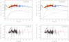 |
Fig. 5 Left-hand column, top panel: rotation curve resulting from the Galactic model MI. The circular velocities due to the three mass components are depicted as dotted lines for the bulge, dashed lines for the disk, and dash-dotted lines for the dark halo. The total circular velocity is represented by the solid curve. The data for the observed rotation curve are presented as red points with orange error bars for the CO tangent-point data (Clemens 1985) and the H I tangent-point data (Fich et al. 1989); and blue points with light blue error bars for the maser sources data (Reid et al. 2014). Bottom panel: velocity residuals between the observed rotation velocities and the total circular model velocities calculated at each radius of the data points. Right-hand column: as for the left-hand column but for the Galactic model MII. |
6. Results and discussions
The best-fitting values for the parameters of both Galactic models MI and MII are summarized in Table 4. Table 5 lists the values for the local dynamical properties resulting from the models, some of which can be compared to the values used as observational constraints and, given the uncertainties, a good overall agreement is observed. Figure 5 shows, in the top panels, the rotation curves resulting from each Galactic model (solid lines) and the curves relative to the contribution of each Galactic component. The data for the observed rotation curve are presented as red points with orange error bars for the CO tangent-point data (Clemens 1985) and for the H I tangent-point data (Fich et al. 1989) and blue points with light blue error bars for the maser sources data (Reid et al. 2014). The bottom panels present the residuals between the observed and the modelled rotation velocities at each radius of the data points. Figure 6 shows the tangent-point data in the plane of observables Vterm − sinl and the curves resultant from the models MI and MII calculated as Vterm = Vrot(R) − V0sinl, with sinl = R/R0. A good agreement between the two curve models and the data can be observed.
In order to compare the goodness of fit between models MI and MII, we use the chi-squared per degree of freedom statistics, χ2/ d.o.f.. Model MI returns χ2/ d.o.f. = 1.85, while model MII provides a fit with χ2/ d.o.f. = 1.46. The relatively better fit provided by model MII can be explained, in part, by its better match to the dip in the observed rotation curve at radii in the interval ~8–10 kpc. As mentioned before, the correspondent dip in the model rotation curve is a consequence of the ring density structure added to the disk model density profile.
In Table 6 we give the correlation matrix of the fitted parameters for both models MI (the lower-left triangle) and MII (the upper-right triangle). In a given correlation matrix, the elements are distributed in the interval [−1; 1], where the value of 1 indicates a perfect correlation and −1 indicates a perfect anti-correlation, whereas 0 corresponds to no correlation. As can be seen from Table 6, the strongest correlations are between parameters associated with a single component, as is the case of the bulge parameters Mb and ab, and also the halo parameters rh and vh. An anti-correlation between the asymptotic circular velocity of the dark halo vh and the disk mass scale factor fmass is observed from model MI; since the dark halo mass must be proportional to vh, this anti-correlation means there is a competition between the disk and the dark halo for the contribution to the dynamical mass in the inner Galaxy. For model MII, anti-correlations are also seen between Mb and fmass, and between fmass and the ring parameter Rring.
6.1. Comparison with studies in the literature
The masses attributed to the bulge in our models are relatively large (Mb ~ 2.6 × 10¹⁰M⊙) compared to other estimates in the literature. This is one cause for the small contribution of the disk component of model MI to the rotational support in the inner Galaxy and also, but to a lesser extent, in model MII (see next section). Most of the studies in the literature find bulge masses of the order of 1 × 10¹⁰M⊙. However, these studies also adopt simple exponential profiles for the disk component with masses in the central regions that are larger than those obtained with our disk models with central density depletion. As pointed out by McMillan (2011), his best-fitting Galactic model presents a stellar mass within the inner 3 kpc of ~2.4 × 10¹⁰M⊙ (the same result obtained in the Flynn et al. 2006 model), which is in close agreement with the bulge mass found by Picaud & Robin (2004) assuming a disk model with a central hole. This is also the same value for the mass of the bulge in the model of Lépine & Leroy (2000), which is also based on a disk with a central density depletion. As described in Sect. 3.1, we based the initial guess values for the bulge parameters on the spheroidal component of the PJL model, which returns a mass inside 3 kpc of ≈2.2 × 10¹⁰M⊙ with a scale radius parameter of 0.4 kpc. The values for the bulge masses Mb and scale radii ab found in our models (see Table 4) reflect the consequence of this choice. The relatively short scale radii cause the rise of the peak in the rotation curves within the inner 1 kpc, as can be seen from Fig. 5. Therefore, according to the PJL star counts model, and also reflected in our models, the bulge is an important mass component in the central region of the Galaxy and its contribution to the model rotation curve is dominant at these radii. Our models return stellar masses enclosed within the inner 3 kpc of 2.7 × 10¹⁰M⊙ (model MI, that is 1.98 × 10¹⁰M⊙ owing to the bulge and 0.72 × 10¹⁰M⊙ owing to the stellar thin and thick disks), and 3 × 10¹⁰M⊙ (model MII, that is 1.98 × 10¹⁰M⊙ owing to the bulge and 1.02 × 10¹⁰M⊙ owing to the stellar thin and thick disks). We can therefore argue about the tendency of the disk models with central holes to redistribute the mass in the central regions from the disk to the bulge without significantly altering the total stellar mass in such regions.
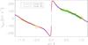 |
Fig. 6 Tangent-point data from Clemens (1985; green circles) and Fich et al.1989; orange circles). The tangent velocity curves resultant from model MI (blue curve) and model MII (red curve) are also plotted. |
The resulting disk stellar mass (thin disk + thick disk) is 3.2 × 10¹⁰M⊙ from model MI and 4.74 × 10¹⁰M⊙ from model MII. As a comparison, Flynn et al. (2006, and references therein) argue that models with disk scale lengths in the range 2–2.6 kpc, based on studies of the Galactic emission in the near-infrared or studies of the local stellar distribution, correspond to disk stellar masses in the range 3.6–5.4 × 10¹⁰M⊙. The total stellar mass (bulge + thin disk + thick disk) of 5.81 × 10¹⁰M⊙ from model MI is close to the interval of 4.85–5.5 × 10¹⁰M⊙ estimated by Flynn et al. (2006), and the total stellar mass of 7.37 × 10¹⁰M⊙ from model MII is relatively close to the best-fitting value of 6.61 × 10¹⁰M⊙ in the model by McMillan (2011). The disk mass in the gaseous form, which is already corrected for the mass contribution of helium, is 1.42 × 10¹⁰M⊙ from model MI and 2.1 × 10¹⁰M⊙ from model MII. The total baryonic mass (stellar + gas) from the models are 7.23 × 10¹⁰M⊙ (model MI) and 9.47 × 10¹⁰M⊙ (model MII). These values are somewhat larger than the “back of the envelope” estimate by Flynn et al. (2006) of 6.1 ± 0.5 × 10¹⁰M⊙, but are compatible with the masses (bulge + disk) of 7–8.2 × 10¹⁰M⊙ found in the models by Irrgang et al. (2013), for instance.
Table 5 also lists the values of the Oort’s constants A and B resulting from the models. Although these constants were not used as observational constraints in the modelling process, their returned values from model MI agree with those estimated in the literature (e.g. Feast & Whitelock 1997). The steeper gradient of the rotation curve at the solar Galactic radius R0 causes the deviation of the Oort’s constants of model MII from their common estimated values. The local escape velocities of 452 km s-1 from model MI and 550 km s-1 from model MII are close and within the 90% confidence interval of 492–587 km s-1 as determined by Piffl et al. (2014b).
6.2. The disk support to the rotation curve
The disk mass scale factor fmass of model MI implies no increase of the originally modelled disk mass. Although returning local surface densities that are compatible with the observed densities that are used as constraints, within the adopted uncertainties, the model MI returns a dynamical mass for the Galactic disk that moderately contributes to the total rotation curve in the inner Galaxy. Sackett (1997), based on a set of Galactic observational constraints, verified that the “maximal disk hypothesis” that is commonly applied to external spiral galaxies also gives a maximal disk when applied to the Milky Way. According to this definition, to be maximal, the exponential disk must provide 85% ± 10% of the total rotation velocity of the galaxy at the radius R = 2.2Rd, where the rotation curve of the disk presents a peak (Rd is the exponential disk scale length). Since our disk models are no longer simple exponentials, we just compare the peak rotation speed of the disk with the total rotation speed at the same radius. From Fig. 5, the peak in the rotation curve of the disk occurs at R ~ 7 kpc for both models MI and MII. We estimate that the disk of model MI is responsible for only 64% of the total circular velocity Vc(R = 7 kpc), which puts it in the condition of a “sub-maximal” disk, however.
On the other hand, the mass scale factor of model MII increases the disk mass by 49% of its original value. This increase in the disk mass is a consequence of the addition of the ring density structure to the density profile of the disk (see Sect. 6.3). Once the solar orbit radius is sitting inside the valley of the ring density feature (near the minimum density, see Fig. 8), to maintain the local disk surface density value within the range determined by the observations, the underlying surface densities at the other radii are proportionally increased. For instance, if it were not for the presence of the ring density giving a local disk surface density of Σ0d = 61M⊙ pc-2 (cf. Table 5), the disk mass of model MII would return Σ0d = 90M⊙ pc-2 instead. We estimate that the disk of model MII contributes with 78% of the total circular velocity at R = 7 kpc, putting it within the limit for a “maximal disk” condition. Therefore, compared with model MI, the disk of model MII contributes more expressively to the inner rotation curve of the Galaxy, giving rise to a less important dark halo component at such regions. It is still important to note that the conclusion by Sackett (1997) about the Galaxy supporting a maximal disk was based, among several observational constraints, on a local disk surface density with a value similar to that used in the present work. But Sackett adopted a local circular velocity of V0 = 210 ± 25 km s-1, while our adopted V0 of 230 km s-1 sits closer to the high side of such interval. Considering now the total rotation supplied by the mass from both bulge and disk, ~82% and 93% of the total circular velocity at R = 7 kpc are provided by the baryonic matter from models MI and MII, respectively.
6.3. The ring structure
In Sect. 3.3, we give some arguments about our reasons for considering an alternative disk model that incorporates a ring density structure near the solar Galactic radius. In terms of the observational data treated in this work, we argue that the apparent velocity dip in the rotation curve of the maser sources, in the radial interval of ~7–11 kpc (compared to a flat rotation curve Vc(R) = V0, for example), can be associated with a ring-like density structure of the type that we consider here. Before modelling such a ring structure, however, it is recommended that we check the reliability of the above-mentioned velocity dip. Indeed, correlations between distance uncertainties and velocity uncertainties could create false trends in the plot of the rotation curve. Since the velocity dip of the rotation curve is traced by the maser sources, we restrict ourselves to these data in the following analysis. For each maser source, we decompose the uncertainty on the azimuthal velocity Vφ, σVφ, into two parts: one component is formed by the combination of the uncertainty on the heliocentric radial velocity, the uncertainties on the two components of the proper motion, and the uncertainties on the solar motion; the second component is solely due to the uncertainty on the distance of the source σd that is derived from the uncertainty on its parallax. We express this second component as σVφ(σd). To verify how much the correlations between the uncertainties on the velocities Vφ and the uncertainties on the distances d affect the velocity dip of the rotation curve, we compute, for each maser source, the difference in velocities (Vφ + σVφ(σd)) − (Vφ − σVφ(σd)) = 2σVφ(σd), and compare this difference to the magnitude of the velocity dip Vdip. From the rotation curve in Fig. 5, we estimate Vdip ≈ 12 km s-1. The comparison between 2σVφ(σd) and Vdip for the maser sources in the interval 7 kpc ≤ R ≤ 11 kpc is shown in Fig. 7. About 80% of the sources present 2σVφ(σd) ≤ 5 km s-1, which is much smaller than Vdip. This result seems to indicate that the correlations between distance uncertainties and velocity uncertainties are not able to create a false trend in the rotation curve, which might appear as a dip in the velocity profile. In other words, the velocity dip in the radial interval 7−11 kpc seems to be a real feature of the observed rotation curve.
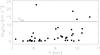 |
Fig. 7 Comparison of the rotation velocity difference 2σVφ(σd) (black circles; see text for details) with the velocity dip Vdip (horizontal line) for the maser sources in the radial interval comprised by the dip of the rotation curve. |
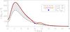 |
Fig. 8 Surface density radial profile for the disks of model MI (dashed curve) and model MII (red solid curve). The black solid curve represents a disk with mass equivalent to that from model MII but without the ring density structure. The shaded area in light grey emphasizes the resulting difference in mass between the disks from both models. The blue point denotes the pair (R0; Σ0d). |
The ring density structure associated with the velocity dip in the rotation curve of model MII, whose parameters (Aring, βring, Rring) are given in Table 4, is depicted in Fig. 8 along with the radial profile for the surface density of the disk from the same model (red curve). The surface density of a disk with equivalent mass to that from model MII, but without the ring structure, is shown by the curve in the black solid line. The ring is formed by a minimum density at the radius of 8.3 kpc, a maximum at 9.8 kpc, and the node radius Rring = 8.9 kpc, which is also the radius of the minimum point in the dip of the modelled rotation curve. The amplitude of the minimum is ≈−0.34 times the density at the same radius of the equivalent disk without the ring. The blue point in Fig. 8 indicates the approximately common value of Σ0d returned from both models MI (indicated by the curve in dashed line) and model MII (red curve) at the solar radius R0. As anticipated in Sects. 3.3 and 6.2, the ring structure causes the rescale of the disk total mass from model MII to a value as large as ~48% of the disk mass from model MI. This increase in mass can be checked out by observing the area highlighted in light grey between the Σ(R) curves of model MI and the equivalent disk of model MII in Fig. 8. The above result is dependent on the scale length measured for the disk of Model MII. The ring structure does not alter the global scale length of the disk, i.e. the global disk scale length of Model MII is the same of model MI. Then the above-quoted increase in the disk mass is satisfied. However, the ring tends to decrease the scale length of the Σ(R) distribution mainly in the radial range of its influence, that is 7 ≲ R ≲ 11 kpc. Once the disk scale length is estimated using this shorter interval of radius, the above considerations of mass increase might not be appropriate.
The density bump at R ~ 9.8 kpc induced by the ring (see Fig. 8) can also be a matter of debate. In fact, the amplitude of this local maximum of density may be too exaggerated, which is a consequence of the form chosen for the ring potential in Eq. (22). Regardless of the true amplitude of the density bump, the question about its plausibility in the observational point of view still needs to be answered. We argue here that since the ring structure was modelled over both stellar and gaseous components, part of such density bump must be associated with the hydrogen distribution of the disk. And indeed, recent works by Nakanishi & Sofue (2016) and Sofue & Nakanishi (2016) clearly show an increase in the hydrogen density of the disk at radii slightly beyond 10 kpc. A stellar counterpart of the density bump, if it existed, would be more difficult to notice for various reasons, such as the relative position of the Sun in the ring structure and the beginning of the flare of the stellar disk just after the solar radius. We believe that estimates of the stellar surface density in a great coverage of the Galactic disk exterior to the solar circle (not only in radius but also in azimuth and height from the plane) are still needed to confirm or refute the existence of the stellar ring structure. In a positive case, our ring model could serve as a starting point to the study of the properties of such a structure in the Galactic disk. These are some aspects that make model MII an “alternative model”, in the sense treated in this work.
7. Conclusions
We have developed models for the axisymmetric mass distribution of the Galaxy with the aim to derive fully analytical descriptions of its associated three-dimensional gravitational potential. We followed an approach that intentionally expends more effort in a detailed modelling of the disk component. Based on photometric constraints for the stellar distribution in the disk given by the Galactic infrared star counts model of PJL and on the observed distribution of atomic and molecular hydrogen gas, we derived an “empirical basis” for the structural parameters (scale length, scale height, and radial scale of the disk central hole) of the thin and thick stellar disks and the H I and H2 disks subcomponents. With a priori values for the masses of each disk, based on the most recent determinations of the local stellar and gaseous disk surface densities, we constructed versions of Miyamoto-Nagai disks for each disk subcomponent mass model. The method follows the approach developed by Smith et al. (2015), but we allow ourselves to use the Miyamoto-Nagai disk models of higher orders 2 and 3 beside the commonly used model of order 1 (Miyamoto & Nagai 1975). Along with parametric models for the bulge and an extra unknown spherical mass component which for “convenience” we refer to by the often-used term dark halo, we searched for the dynamical mass of each Galactic component by fitting the models to the kinematic constraints given by the observed rotation curve and some local Galactic measured properties.
We have shown that a disk model that includes a ring density pattern beyond but very close to the solar orbit radius is able to better reproduce an observed local dip in the Galactic rotation curve centred at R ~ 9.0 kpc; such dip is naturally explained by a ring density structure composed of a minimum followed by a maximum density of similar amplitudes. Furthermore, the model with the ring structure allows a more massive disk to increasingly contribute to the rotational support of the Galaxy inside the solar circle, thereby helping the Milky Way to satisfy the condition to be considered a “maximal disk” galaxy. The model with the ring structure also relies on a numerical study of the stellar disk, where a ring density structure develops as a consequence of interactions between the stars and the galactic spiral arms in resonance at the co-rotation radius (BLJ). Since we still have no information about the three-dimensional structure of this ring density feature, we had to make crude approximations for the vertical profile of its associated gravitational potential. We believe that, with the forthcoming data of the GAIA mission (Perryman et al. 2001), the ring structure in the disk may become an object of examination and, in the case of confirmation of its existence, constraints on its three-dimensional distribution in the global disk structure will help us to create more realistic disk models.
The method we applied for the construction of the disk mass model and its associated gravitational potential is very flexible in the sense that for any set of structural parameters, disks of different masses can be generated. We emphasize at this point that the models of Galactic gravitational potential presented in this work are aimed to be used in studies of orbits in the disk that do not extend too far away in Galactic radii and do not reach great heights above the disk mid-plane. These limitations are imposed by the spatial coverage of the observational data used to constrain the models in the sense that for radii greater than ~2R0 (the maximum radius of the data used for the rotation curve) and heights | z | ≳ 3 kpc, we do not guarantee that our models return confident representations of the Galactic potential, but they may provide reasonable representations at least. Also in this respect, no constraint on the mass at large radii is adopted here, as has been made by some studies that derive properties of the dark halo by requiring distant halo stars to be bound to the Milky Way potential. We included a density component associated with a spherical logarithmic potential to explain the observed rotation curve data at radii R0 ≲ R ≲ 2R0. As pointed out by Dehnen & Binney (1998), however, instead of a distinct physical component, it is possible that we are measuring the dynamical effects of a disk and/or a bulge in which the mass-to-light ratio of their content strongly increases from the centre to the Galactic outskirts.
The models for the three-dimensional gravitational potential of the Galaxy presented in this work, as they are fully analytical and easy to obtain the associated gravitational force-field at any point, are suited for fast and accurate calculations of orbits of stellar-like objects belonging to the main populations of the Galactic disk. In a forthcoming study, we aim to present an application of these new potential models to a description of the distributions of orbital parameters for samples of Galactic open clusters and some expected correlations with their chemical abundance patterns.
The tangent velocity data in Table 2 of Clemens (1985) were corrected for 3 km s-1 line width, and a correction of 7 km s-1 for the LSR peculiar motion in the azimuthal direction was used in the calculation of the rotation velocities, as proposed by the author in the above-cited paper.
Acknowledgments
We acknowledge the referee whose comments and suggestions have significantly improved the present paper. D.A.B. received financial support for this work from the Brazilian research agency CAPES (Coordenação de Aperfeiçoamento de Pessoal de Nível Superior) through the PNPD postdoctoral programme.
References
- Allen, C., & Santillan, A. 1991, Rev. Mex. Astron. Astrofis., 22, 255 [NASA ADS] [Google Scholar]
- Amôres, E. B., & Lépine, J. R. D. 2005, AJ, 130, 659 [NASA ADS] [CrossRef] [Google Scholar]
- Amôres, E. B., Lépine, J. R. D., & Mishurov, Y. N. 2009, MNRAS, 400, 1768 [NASA ADS] [CrossRef] [Google Scholar]
- Bahcall, J. N., & Soneira, R. M. 1980, ApJS, 44, 73 [NASA ADS] [CrossRef] [Google Scholar]
- Bahcall, J. N., Flynn, C., & Gould, A. 1992, ApJ, 389, 234 [NASA ADS] [CrossRef] [Google Scholar]
- Barros, D. A., Lépine, J. R. D., & Junqueira, T. C. 2013, MNRAS, 435, 2299 (BLJ) [NASA ADS] [CrossRef] [Google Scholar]
- Bienaymé, O., Soubiran, C., Mishenina, T. V., Kovtyukh, V. V., & Siebert, A. 2006, A&A, 446, 933 [NASA ADS] [CrossRef] [EDP Sciences] [Google Scholar]
- Binney, J., & Dehnen, W. 1997, MNRAS, 287, L5 [NASA ADS] [Google Scholar]
- Binney, J., & Merrifield, M. 1998, Galactic Astronomy (Princeton University Press) [Google Scholar]
- Binney, J., & Tremaine, S. 2008, Galactic Dynamics, 2nd edn. (Princeton University Press) [Google Scholar]
- Bovy, J., & Rix, H.-W. 2013, ApJ, 779, 115 [NASA ADS] [CrossRef] [Google Scholar]
- Bovy, J., Rix, H.-W., & Hogg, D. W. 2012, ApJ, 751, 131 [NASA ADS] [CrossRef] [Google Scholar]
- Burton, W. B. 1976, ARA&A, 14, 275 [NASA ADS] [CrossRef] [Google Scholar]
- Caetano, T. C., Dias, W. S., Lépine, J. R. D., et al. 2015, New Astron., 38, 31 [NASA ADS] [CrossRef] [Google Scholar]
- Caldwell, J. A. R., & Ostriker, J. P. 1981, ApJ, 251, 61 [NASA ADS] [CrossRef] [Google Scholar]
- Caproni, A., Monteiro, H., & Abraham, Z. 2009, MNRAS, 399, 1415 [NASA ADS] [CrossRef] [Google Scholar]
- Chemin, L., Renaud, F., & Soubiran, C. 2015, A&A, 578, A14 [NASA ADS] [CrossRef] [EDP Sciences] [Google Scholar]
- Clemens, D. P. 1985, ApJ, 295, 422 [NASA ADS] [CrossRef] [Google Scholar]
- de Vaucouleurs, G. 1977, AJ, 82, 456 [NASA ADS] [CrossRef] [Google Scholar]
- Dehnen, W., & Binney, J. 1998, MNRAS, 294, 429 [NASA ADS] [CrossRef] [Google Scholar]
- Dias, W. S., & Lépine, J. R. D. 2005, ApJ, 629, 825 [NASA ADS] [CrossRef] [Google Scholar]
- Dias, W. S., Monteiro, H., Caetano, T. C., et al. 2014, A&A, 564, A79 [NASA ADS] [CrossRef] [EDP Sciences] [Google Scholar]
- Feast, M., & Whitelock, P. 1997, MNRAS, 291, 683 [NASA ADS] [CrossRef] [Google Scholar]
- Fich, M., Blitz, L., & Stark, A. A. 1989, ApJ, 342, 272 [NASA ADS] [CrossRef] [Google Scholar]
- Flynn, C., Sommer-Larsen, J., & Christensen, P. R. 1996, MNRAS, 281, 1027 [NASA ADS] [CrossRef] [Google Scholar]
- Flynn, C., Holmberg, J., Portinari, L., Fuchs, B., & Jahreiß, H. 2006, MNRAS, 372, 1149 [NASA ADS] [CrossRef] [MathSciNet] [Google Scholar]
- Freeman, K. C. 1970, ApJ, 160, 811 [NASA ADS] [CrossRef] [Google Scholar]
- Freudenreich, H. T. 1998, ApJ, 492, 495 [NASA ADS] [CrossRef] [Google Scholar]
- Gilks, W., Richardson, S., & Spiegelhalter, D. 1996, Markov chain Monte Carlo in practice (London: Chapman and Hall) [Google Scholar]
- Hernquist, L. 1990, ApJ, 356, 359 [NASA ADS] [CrossRef] [Google Scholar]
- Hessman, F. V. 2015, A&A, 579, A123 [NASA ADS] [CrossRef] [EDP Sciences] [Google Scholar]
- Holmberg, J., & Flynn, C. 2000, MNRAS, 313, 209 [NASA ADS] [CrossRef] [Google Scholar]
- Holmberg, J., & Flynn, C. 2004, MNRAS, 352, 440 [NASA ADS] [CrossRef] [Google Scholar]
- Honma, M., Nagayama, T., Ando, K., et al. 2012, PASJ, 64, 136 [NASA ADS] [CrossRef] [Google Scholar]
- Irrgang, A., Wilcox, B., Tucker, E., & Schiefelbein, L. 2013, A&A, 549, A137 [NASA ADS] [CrossRef] [EDP Sciences] [Google Scholar]
- Johnson, D. R. H., & Soderblom, D. R. 1987, AJ, 93, 864 [NASA ADS] [CrossRef] [Google Scholar]
- Jurić, M., Ivezić, Ž., Brooks, A., et al. 2008, ApJ, 673, 864 [NASA ADS] [CrossRef] [MathSciNet] [Google Scholar]
- Kalberla, P. M. W., & Dedes, L. 2008, A&A, 487, 951 [NASA ADS] [CrossRef] [EDP Sciences] [Google Scholar]
- Kalberla, P. M. W., Dedes, L., Kerp, J., & Haud, U. 2007, A&A, 469, 511 [NASA ADS] [CrossRef] [EDP Sciences] [Google Scholar]
- Kalberla, P. M. W., Kerp, J., Dedes, L., & Haud, U. 2014, ApJ, 794, 90 [NASA ADS] [CrossRef] [Google Scholar]
- Kormendy, J. 1977, ApJ, 217, 406 [NASA ADS] [CrossRef] [Google Scholar]
- Kroese, D. P., Porotsky, S., & Rubinstein, R. Y. 2006, Methodology and Computing in Applied Probability, 8, 383 [Google Scholar]
- Kuijken, K., & Gilmore, G. 1991, ApJ, 367, L9 [NASA ADS] [CrossRef] [Google Scholar]
- Kuzmin, C. G. 1956, Astron. Zh, 33, 27 [Google Scholar]
- Lépine, J. R. D., & Leroy, P. 2000, MNRAS, 313, 263 [NASA ADS] [CrossRef] [Google Scholar]
- Lépine, J. R. D., Mishurov, Y. N., & Dedikov, S. Y. 2001, ApJ, 546, 234 [NASA ADS] [CrossRef] [Google Scholar]
- Li, Z., Gerhard, O., Shen, J., Portail, M., & Wegg, C. 2016, ApJ, 824, 13 [NASA ADS] [CrossRef] [Google Scholar]
- López-Corredoira, M., Cabrera-Lavers, A., Gerhard, O. E., & Garzón, F. 2004, A&A, 421, 953 [NASA ADS] [CrossRef] [EDP Sciences] [Google Scholar]
- Lozinskaya, T. A., & Kardashev, N. S. 1963, Soviet Ast., 7, 161 [NASA ADS] [Google Scholar]
- Malkin, Z. 2013, in IAU Symp. 289, ed. R. de Grijs, 406 [Google Scholar]
- Martins, L. P., Coelho, P., Caproni, A., & Vitoriano, R. 2014, MNRAS, 442, 1294 [NASA ADS] [CrossRef] [Google Scholar]
- McMillan, P. J. 2011, MNRAS, 414, 2446 [NASA ADS] [CrossRef] [Google Scholar]
- McMillan, P. J., & Binney, J. J. 2010, MNRAS, 402, 934 [NASA ADS] [CrossRef] [Google Scholar]
- Miyamoto, M., & Nagai, R. 1975, PASJ, 27, 533 [NASA ADS] [Google Scholar]
- Monteiro, H., & Dias, W. S. 2011, A&A, 530, A91 [NASA ADS] [CrossRef] [EDP Sciences] [Google Scholar]
- Monteiro, H., Dias, W. S., & Caetano, T. C. 2010, A&A, 516, A2 [NASA ADS] [CrossRef] [EDP Sciences] [Google Scholar]
- Nakanishi, H., & Sofue, Y. 2006, PASJ, 58, 847 [NASA ADS] [Google Scholar]
- Nakanishi, H., & Sofue, Y. 2016, PASJ, 68, 5 [NASA ADS] [CrossRef] [Google Scholar]
- Perryman, M. A. C., de Boer, K. S., Gilmore, G., et al. 2001, A&A, 369, 339 [NASA ADS] [CrossRef] [EDP Sciences] [Google Scholar]
- Picaud, S., & Robin, A. C. 2004, A&A, 428, 891 [NASA ADS] [CrossRef] [EDP Sciences] [Google Scholar]
- Piffl, T., Binney, J., McMillan, P. J., et al. 2014a, MNRAS, 445, 3133 [NASA ADS] [CrossRef] [Google Scholar]
- Piffl, T., Scannapieco, C., Binney, J., et al. 2014b, A&A, 562, A91 [NASA ADS] [CrossRef] [EDP Sciences] [Google Scholar]
- Polido, P., Jablonski, F., & Lépine, J. R. D. 2013, ApJ, 778, 32 (PJL) [NASA ADS] [CrossRef] [Google Scholar]
- Read, J. I. 2014, J. Phys. G Nucl. Phys., 41, 063101 [NASA ADS] [CrossRef] [Google Scholar]
- Reid, M. J., & Brunthaler, A. 2004, ApJ, 616, 872 [NASA ADS] [CrossRef] [Google Scholar]
- Reid, M. J., Menten, K. M., Zheng, X. W., et al. 2009, ApJ, 700, 137 [NASA ADS] [CrossRef] [Google Scholar]
- Reid, M. J., Menten, K. M., Brunthaler, A., et al. 2014, ApJ, 783, 130 [Google Scholar]
- Robin, A. C., Reylé, C., Derrière, S., & Picaud, S. 2003, A&A, 409, 523 [NASA ADS] [CrossRef] [EDP Sciences] [Google Scholar]
- Rodriguez-Fernandez, N. J., & Combes, F. 2008, A&A, 489, 115 [NASA ADS] [CrossRef] [EDP Sciences] [Google Scholar]
- Rohlfs, K., & Kreitschmann, J. 1988, A&A, 201, 51 [NASA ADS] [Google Scholar]
- Rubinstein, R. Y. 1997, Eur. J. Oper. Res., 99, 89 [Google Scholar]
- Rubinstein, R. Y. 1999, Methodology and Computing in Applied Probability, 1, 127 [NASA ADS] [CrossRef] [Google Scholar]
- Sackett, P. D. 1997, ApJ, 483, 103 [NASA ADS] [CrossRef] [Google Scholar]
- Sanders, D. B., Solomon, P. M., & Scoville, N. Z. 1984, ApJ, 276, 182 [NASA ADS] [CrossRef] [Google Scholar]
- Schmidt, M. 1956, Bull. Astron. Inst. Netherlands, 13, 15 [Google Scholar]
- Schönrich, R., Binney, J., & Dehnen, W. 2010, MNRAS, 403, 1829 (SBD) [NASA ADS] [CrossRef] [Google Scholar]
- Skilling, J. 2004, in AIP Conf. Ser. 735, eds. R. Fischer, R. Preuss, & U. V. Toussaint, 395 [Google Scholar]
- Skrutskie, M. F., Cutri, R. M., Stiening, R., et al. 2006, AJ, 131, 1163 [NASA ADS] [CrossRef] [Google Scholar]
- Smith, R., Flynn, C., Candlish, G. N., Fellhauer, M., & Gibson, B. K. 2015, MNRAS, 448, 2934 [NASA ADS] [CrossRef] [Google Scholar]
- Sofue, Y., & Nakanishi, H. 2016, PASJ, 68, 63 [NASA ADS] [CrossRef] [Google Scholar]
- Sofue, Y., Honma, M., & Omodaka, T. 2009, PASJ, 61, 227 [NASA ADS] [Google Scholar]
- Spitzer, L. 1968, Diffuse matter in space (New York: Interscience Publication) [Google Scholar]
- Toomre, A. 1963, ApJ, 138, 385 [NASA ADS] [CrossRef] [Google Scholar]
- Zhang, X. 1996, ApJ, 457, 125 [NASA ADS] [CrossRef] [Google Scholar]
Appendix A: Parameters and relations for Miyamoto-Nagai disks models
In this Appendix, we present the variations of the ratios M/Md and a/Rdexp as a function of b/Rdexp (M, a, and b are the free parameters of the Miyamoto-Nagai disks) and the relations between b/Rdexp and hz/Rdexp for each disk subcomponent, calculated in the same way as in Smith et al. (2015). Here, for simplicity, we denote the exponential scale length Rdexp simply as Rd. As stated in the main text, these relations are intended to help in the construction of Miyamoto-Nagai disks models for disks of any mass Md, scale length Rd and scale height hz, which can be different from those modelled in the present work. The relations presented for the thin stellar disk, the H I and H2 disks, are for models of disks with density depressions in their central regions, while for the thick stellar disk the relations are correspondent to simple radially exponential disks. Regarding the vertical density distributions, the models for the thin and thick stellar disks consider exponential density decays with the increase of the height above the mid-plane and, for the H I and H2 disks, a Gaussian density profile is adopted for the models. We emphasize here that such relations are constructed for models of three MN-disk combinations, which are model 3 for the thin disk and the H2 disk (Eqs. (11) and (16)), model 1 for the thick disk (Eqs. (9) and (14)), and model 2 for the H I disk (Eqs. (10) and (15)).
Figure A.1 shows the variation of the thickness ratio b/Rd as a function of the ratio hz/Rd for the thin and thick stellar disks and the H I and H2 disks subcomponents. Filled circles in the figure represent the calculated relations in the way described in Sect. 2.2.3 of the main text. The solid lines represent 4th-order polynomial fits to the distribution of points associated with each calculated relation and are given in the form 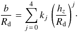 (A.1)The values of the coefficients k0–k4 of the above relation, and for each disk subcomponent, are given in Table A.1.
Figure A.2 shows the variations of the ratios Mi/Md (left-hand panel) and ai/Rd (right-hand panel) as a function of the variation of the ratio b/Rd (filled circles), calculated for the modelling of the thin stellar disk. The subscript i = 1, 2, 3 denotes each one of the three MN-disks used in the combination. The points corresponding to the ratio b/Rd = 0
denote the values of Mi and ai, which are the best-fitting solutions for the three Toomre-Kuzmin disks combination. The solid lines in each panel of Fig. A.2 represent 4th-order polynomial fits to the points that describe the variations of M/Md and a/Rd as a function of b/Rd. Each parameter  or
or  can then be written as a function of b/Rd in the form
  (A.2)The values of the coefficients c0–c4 for the three MN-disk fit models to the thin stellar disk for the range of thicknesses b/Rd from 0 to 1.5, are given in Table A.2.
Analogously, the relations between (Mi/Md; ai/Rd) and b/Rd for the thick stellar disk, the H I disk, and the H2 disk are shown in Figs. A.3–A.5, respectively. The solid lines in these figures also represent 4th-order polynomial fits to the distribution of points shown as filled circles, and are all also written in the form of Eq. (A.2). The coefficients cj are given in Tables A.3–A.5, for the thick disk, the H I disk, and the H2 disk, respectively.
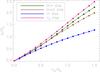 |
Fig. A.1 Variation of the thickness ratio b/Rd as a function of the ratio hz/Rd, for the thin and thick stellar disks and the H I and H2 disks subcomponents. Filled circles represent the optimal solutions found after the application of the cross-entropy algorithm, as described in Sect. 2.2.2 of the main text. Solid lines represent 4th-order polynomial fits to the distribution of points associated with each calculated relation. |
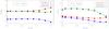 |
Fig. A.2 Left-hand panel: variation of the three mass parameters of the three MN-disk models as a function of the disk thickness ratio b/Rd, for the modelling of the thin stellar disk. Right-hand panel: variation of the three scale-length parameters as a function of the ratio b/Rd. In the panels, the points represent the optimal solutions found after the application of the cross-entropy algorithm. Solid lines are fourth-order polynomial fits to the distribution of points. |
Appendix B: Radial and vertical components of the gradients of the gravitational potential models for each Galactic component
Here we give the explicit forms for the radial and vertical components of the gradients of the gravitational potential expressions modelled for each Galactic mass component, which can be used in the construction of the gravitational force-field model of the Galaxy.
Appendix B.1: The Miyamoto-Nagai disks
In the following, we write the components of the gradients for the three models of Miyamoto-Nagai gravitational potential, which are expressed by Eqs. (14)–(16) in the main text. In all expressions, we use the identity .
Appendix B.1.1: Model 1 (Eq. (14))
![\appendix \setcounter{section}{2} \begin{eqnarray} \label{eq:dPhi_MN1_dR} &&\frac{\partial\Phi_{\mathrm{MN}_{1}}}{\partial R}=\frac{GMR}{\left[R^{2}+\left(a+\zeta\right)^{2}\right]^{3/2}} \\ \label{eq:dPhi_MN1_dz} &&\frac{\partial\Phi_{\mathrm{MN}_{1}}}{\partial z}=\frac{GM\,z\left(a+\zeta\right)}{\zeta\left[R^{2}+\left(a+\zeta\right)^{2}\right]^{3/2}}\cdot \end{eqnarray}](/articles/aa/full_html/2016/09/aa27535-15/aa27535-15-eq442.png)
Appendix B.1.2: Model 2 (Eq. (15))
![\appendix \setcounter{section}{2} \begin{eqnarray} \label{eq:dPhi_MN2_dR} &&\frac{\partial\Phi_{\mathrm{MN}_{2}}}{\partial R}=\frac{GMR}{\left[R^{2}+\left(a+\zeta \right)^{2}\right]^{5/2}}\left[R^{2}+\left(a+\zeta\right)^{2}+3a\left(a+\zeta\right)\right] \\ \label{eq:dPhi_MN2_dz} &&\frac{\partial\Phi_{\mathrm{MN}_{2}}}{\partial z}=\frac{GM\,z}{\zeta\left[R^{2}+\left(a+\zeta \right)^{2}\right]^{5/2}}\left[\zeta R^{2}+\left(a+\zeta\right)^{3}+ 2a\left(a+\zeta\right)^{2}\right]\cdot \end{eqnarray}](/articles/aa/full_html/2016/09/aa27535-15/aa27535-15-eq443.png)
Appendix B.1.3: Model 3 (Eq. (16))
![\appendix \setcounter{section}{2} \begin{eqnarray} \label{eq:dPhi_MN3_dR} \frac{\partial\Phi_{\mathrm{MN}_{3}}}{\partial R}=\frac{GMR}{\left[R^{2}+\left(a+\zeta \right)^{2}\right]^{7/2}}\left\{\left[R^{2}+\left(a+\zeta\right)^{2}\right]^{2}+3a\zeta R^{2} \right.\nonumber\\ + \left. 3a\left(a+\zeta\right)^{3}+4a^{2}\left(a+\zeta\right)^{2}+2a^{2}R^{2} \right\} \end{eqnarray}](/articles/aa/full_html/2016/09/aa27535-15/aa27535-15-eq444.png)
![\appendix \setcounter{section}{2} \begin{eqnarray} \label{eq:dPhi_MN3_dz} \frac{\partial\Phi_{\mathrm{MN}_{3}}}{\partial z}=\frac{GM\,z}{\zeta\left[R^{2}+\left(a+\zeta \right)^{2}\right]^{7/2}}\left\{\left\{\left[R^{2}+\left(a+\zeta\right)^{2}\right]^{2}-2a^{2}R^{2} \right.\right.\nonumber\\ + \left.\left. a\zeta R^{2}\right\}(a+\zeta)+2a^{2}\left(a+\zeta\right)^{3}+2a\left(a+\zeta\right)^{4}-aR^{4} \right\}\cdot \end{eqnarray}](/articles/aa/full_html/2016/09/aa27535-15/aa27535-15-eq445.png)
Appendix B.2: The bulge (Eq. (19))
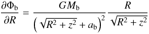
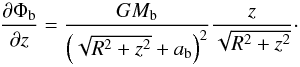
Appendix B.3: The dark halo (Eq. (20))
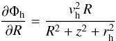
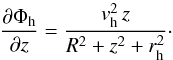
Appendix B.4: The ring potential (Eq. (22))
With the functions ϕR(R) and ϕz(z) given in Eq. (22), we have ![\appendix \setcounter{section}{2} \begin{equation} \label{eq:dPhiring_dR} \frac{\partial\Phi_{\rm ring}}{\partial R}=\frac{A_{\rm ring}\,\beta_{\rm ring}\,\varphi_{z}(z)}{R}\,\mathrm{sech}\,\phi\left[ \tanh^{2}\phi - \mathrm{sech}^{2}\phi \right] \end{equation}](/articles/aa/full_html/2016/09/aa27535-15/aa27535-15-eq452.png) (B.11)
(B.11)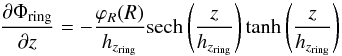 (B.12)with the argument
  in Eq. (B.11).
All Tables
Structural parameters, local surface densities, and masses of the disk components taken as observational prior information to the Milky Way modelling.
Models of 3 TK-disks that provide the best match to the surface density of each disk subcomponent.
Parameters of the three MN-disk combinations for modelling each subcomponent of the Galactic disk.
Local properties resulting from the models MI and MII for the mass distribution and gravitational potential of the Galaxy.
Correlation matrix for the model parameters: the lower-left triangle for model MI and the upper-right triangle for model MII.
All Figures
|
Fig. 1 Radial profile of the surface density of our “observation-based” model for the Milky Way’s disk. The curves indicate the surface densities of the thin disk (green), thick disk (brown), H I disk (blue), H2 disk (violet), and the total disk (red). |
| In the text | |
|
Fig. 2 Left-hand panel: radial distribution of the surface mass density of the Galactic disk model; the “observation-based” disk model (blue curve) and the resultant from the sum of all the 3 MN-disk combinations fitted to each disk subcomponent (red curve). Right-hand panel: vertical profile of the volume density of the Galactic disk model as a function of the height z from the mid-plane and at three different arbitrary radii: R = 2 kpc (solid lines); R = 8 kpc (R0) (dashed lines); and R = 15 kpc (dotted lines). The blue curves are also related to the “observation-based” disk model and the red curves to the total 3 MN-disk combinations. |
| In the text | |
|
Fig. 3 Contours of iso-densities log ρ for the disk models built in the present work. Left-hand panel: the “observation-based” disk model; right-hand panel: the sum of all three MN-disk combinations fitted to each disk subcomponent. The values of the contours lie in the range log ρ = [−6; +1], with ρ in M⊙ pc-3. |
| In the text | |
|
Fig. 4 Contours of equipotentials in the Galactic meridional plane for the gravitational potential resulting from the disk model composed of combinations of MN-disks, as described in Sect. 2.2.3. The contours of Φd are given in 104 km2 s-2, as indicated in the colourbar. |
| In the text | |
|
Fig. 5 Left-hand column, top panel: rotation curve resulting from the Galactic model MI. The circular velocities due to the three mass components are depicted as dotted lines for the bulge, dashed lines for the disk, and dash-dotted lines for the dark halo. The total circular velocity is represented by the solid curve. The data for the observed rotation curve are presented as red points with orange error bars for the CO tangent-point data (Clemens 1985) and the H I tangent-point data (Fich et al. 1989); and blue points with light blue error bars for the maser sources data (Reid et al. 2014). Bottom panel: velocity residuals between the observed rotation velocities and the total circular model velocities calculated at each radius of the data points. Right-hand column: as for the left-hand column but for the Galactic model MII. |
| In the text | |
|
Fig. 6 Tangent-point data from Clemens (1985; green circles) and Fich et al.1989; orange circles). The tangent velocity curves resultant from model MI (blue curve) and model MII (red curve) are also plotted. |
| In the text | |
|
Fig. 7 Comparison of the rotation velocity difference 2σVφ(σd) (black circles; see text for details) with the velocity dip Vdip (horizontal line) for the maser sources in the radial interval comprised by the dip of the rotation curve. |
| In the text | |
|
Fig. 8 Surface density radial profile for the disks of model MI (dashed curve) and model MII (red solid curve). The black solid curve represents a disk with mass equivalent to that from model MII but without the ring density structure. The shaded area in light grey emphasizes the resulting difference in mass between the disks from both models. The blue point denotes the pair (R0; Σ0d). |
| In the text | |
|
Fig. A.1 Variation of the thickness ratio b/Rd as a function of the ratio hz/Rd, for the thin and thick stellar disks and the H I and H2 disks subcomponents. Filled circles represent the optimal solutions found after the application of the cross-entropy algorithm, as described in Sect. 2.2.2 of the main text. Solid lines represent 4th-order polynomial fits to the distribution of points associated with each calculated relation. |
| In the text | |
|
Fig. A.2 Left-hand panel: variation of the three mass parameters of the three MN-disk models as a function of the disk thickness ratio b/Rd, for the modelling of the thin stellar disk. Right-hand panel: variation of the three scale-length parameters as a function of the ratio b/Rd. In the panels, the points represent the optimal solutions found after the application of the cross-entropy algorithm. Solid lines are fourth-order polynomial fits to the distribution of points. |
| In the text | |
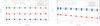 |
Fig. A.3 Same as Fig. A.2, but for the modelling of the thick stellar disk. |
| In the text | |
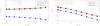 |
Fig. A.4 Same as Fig. A.2, but for the modelling of the H I disk. |
| In the text | |
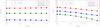 |
Fig. A.5 Same as Fig. A.2, but for the modelling of the H2 disk. |
| In the text | |
Current usage metrics show cumulative count of Article Views (full-text article views including HTML views, PDF and ePub downloads, according to the available data) and Abstracts Views on Vision4Press platform.
Data correspond to usage on the plateform after 2015. The current usage metrics is available 48-96 hours after online publication and is updated daily on week days.
Initial download of the metrics may take a while.