| Issue |
A&A
Volume 689, September 2024
|
|
|---|---|---|
| Article Number | A57 | |
| Number of page(s) | 9 | |
| Section | Galactic structure, stellar clusters and populations | |
| DOI | https://doi.org/10.1051/0004-6361/202348211 | |
| Published online | 30 August 2024 | |
Testing MOND using the dynamics of nearby stellar streams
Kapteyn Astronomical Institute, University of Groningen, Landleven 12, 9747 AD Groningen, The Netherlands
Received:
9
October
2023
Accepted:
18
June
2024
Context. The stellar halo of the Milky Way is built up at least in part from debris from past mergers. The stars from these merger events define substructures in phase space, for example in the form of streams, which are groups of stars that move on similar trajectories. The nearby Helmi streams discovered more than two decades ago are a well-known example. Using 6D phase-space information from the Gaia space mission, recent work showed that the Helmi streams are split into two clumps in angular momentum space. This substructure can be explained and sustained in time if the dark matter halo of the Milky Way takes a prolate shape in the region probed by the orbits of the stars in the streams.
Aims. Here, we explore the behaviour of the two clumps identified in the Helmi streams in a modified Newtonian dynamics (MOND) framework to test this alternative model of gravity.
Methods. We performed orbit integrations of Helmi streams member stars in a simplified MOND model of the Milky Way and using the more sophisticated phantom of RAMSES simulation framework.
Results. We find with both approaches that the two Helmi streams clumps do not retain their identity and dissolve after merely 100 Myr. This extremely short timescale would render the detection of two separate clumps very unlikely in MONDian gravity.
Conclusions. The observational constraints provided by the streams, which MOND fails to reproduce in its current formulation, could potentially also be used to test other alternative gravity models.
Key words: gravitation / Galaxy: kinematics and dynamics / Galaxy: structure
© The Authors 2024
 Open Access article, published by EDP Sciences, under the terms of the Creative Commons Attribution License (https://creativecommons.org/licenses/by/4.0), which permits unrestricted use, distribution, and reproduction in any medium, provided the original work is properly cited.
This article is published in open access under the Subscribe to Open model. Subscribe to A&A to support open access publication.
1. Introduction
A plenitude of empirical evidence points to mass discrepancies in the Universe. Oort (1932) found the luminous matter in the solar vicinity to be insufficient to explain the vertical motions of stars near the Sun, and Zwicky (1933) reported that the velocity dispersion in (clusters of) galaxies was too high for them to stay bound by the visible mass. Ostriker & Peebles (1973) later showed that dynamically cold disks in galaxies are prone to instability unless they are embedded in some potential well, such as a halo of dark matter. Then Rubin et al. (1982) and Bosma (1981) showed that the rotation curves of spiral galaxies remain approximately flat with increasing radius. With the baryonic mass inferred from the Big Bang nucleosynthesis model, the observation of the cosmic microwave background, and present-day inhomogeneity, the need for a boost of the growth rate with invisible mass also arose from cosmology.
The currently preferred cosmological model includes a cosmological constant (Λ) and involves significant amounts of cold dark matter (CDM). The ΛCDM model is supported by a wealth of observational data over many different scales. It faces some challenges on small scales, however, such as the predicted excess of dark satellites (or subhaloes), the so-called missing satellite problem (see e.g. Boylan-Kolchin et al. 2011; Bullock & Boylan-Kolchin 2017; Pawlowski et al. 2017), or the plane-of-satellites problem, where the observed spatial distribution of the Milky Way satellites seems to be too planar in comparison to predictions from simulations (see e.g. Libeskind et al. 2005; Sawala et al. 2023; Garavito-Camargo et al. 2023; Sales et al. 2022 for a review and possible solutions and outstanding problems on the dwarf galaxy scale). Another challenge is the radial acceleration relation (RAR), where the rotation curve of many galaxies can be predicted from the Newtonian gravitational acceleration alone in a universal way (see e.g. Banik & Zhao 2022, and references therein).
An alternative way of considering the hidden-mass hypothesis is that the problem signals a breakdown of Newtonian dynamics in the weak-acceleration regime, defined by a new constant a0, of about 10−10 m s−2, which was found to be appropriate to the tiny accelerations encountered in galaxies beyond the solar radius (Milgrom 1983a; Gaia Collaboration 2021a). Modified Newtonian dynamics (MOND) is able to predict the observation of flat rotation curves, the RAR and the baryonic Tully–Fisher relation, the last of which is a scaling relation between the luminosity and the circular velocity of disk galaxies (Famaey & McGaugh 2012; Milgrom 1983b; Lelli et al. 2016; McGaugh et al. 2016). However, MOND runs into challenges on more cosmological scales and even needs additional dark matter to explain certain observations of galaxy clusters (Sanders 1999; Skordis & Złośnik 2021).
With the increasing number of data on our own Galaxy, especially from the Gaia mission (Gaia Collaboration 2016), more tests of MOND on the Galactic scale can be performed. However, due to the nonlinearity of MOND (i.e. forces are not additive), attempts have been somewhat limited thus far, except for instance the work done by Read & Moore (2005). Some other examples include using the kinematics of stars to model the rotation curve and mass distribution in the Galaxy (Banik & Zhao 2018; Lisanti et al. 2019; Dai et al. 2022; Finan-Jenkin & Easther 2023; Zhu et al. 2023; Sylos Labini et al. 2023) and the modelling of stellar streams (Thomas et al. 2017, 2018; Kroupa et al. 2022) using the phantom of RAMSES patch (PoR, Lüghausen et al. 2015). Stellar streams are the products of the tidal stripping of satellites such as globular clusters or dwarf galaxies. These streams are a great probe of the Galactic mass distribution and potential. Not only are their characteristics dependent on the overall gravitational potential, but the presence of dark satellites (often referred to as subhaloes, predicted to be in the thousands in the case of cold dark matter) can result in gaps, spurs, or other substructures in streams (Ibata et al. 2002; Johnston et al. 2002; Erkal & Belokurov 2015). These features would have to be attributed to interactions with baryonic structures in the case of MOND. Furthermore, tidal streams resulting from globular clusters in MOND will experience an altered internal potential, leading to an asymmetry between the leading and trailing tidal tails (Thomas et al. 2018), which is generally not expected in Newtonian gravity (see Dehnen et al. 2004; Pearson et al. 2017, for more discussion).
The stellar streams identified thus far include the Helmi streams, which cross the solar neighbourhood (Helmi et al. 1999; Koppelman et al. 2019). They are thought to be the debris of a massive dwarf galaxy with a stellar mass of M* ∼ 108 M⊙ that was accreted approximately 5−8 Gyr ago. Its stars are phase-mixed, implying that they do not define spatially tight structures, but that the stars of the streams cross the solar vicinity in different phases of their orbit. They define clumps in velocity space as well as integrals of motion space (see Fig. 1). The latter is defined by (quasi-)conserved quantities along the orbit of the stars, such as their energy and angular momenta. These can be used to dynamically track groups of stars of similar origin (Helmi & de Zeeuw 2000). Dodd et al. (2022, hereafter D22) have shown that the Helmi streams in fact define two distinct clumps in angular-momentum space (Lz − L⊥, where  ). The existence of these two subclumps has been confirmed by a clustering algorithm using both Gaia EDR3 (Lövdal et al. 2022; Ruiz-Lara et al. 2022) and the more recent Gaia DR3 dataset (Dodd et al. 2023). The stellar populations of these two clumps are indistinguishable, which means that they must have originated in the same system. D22 demonstrated that the two clumps in (Lz − L⊥) space are able to survive in time as such if the Galactic dark matter halo has a prolate shape with axis ratio qρ ∼ 1.2. In this case, one of the clumps is placed on the Ωϕ:Ωz = 1:1 orbital resonance.
 |
Fig. 1. Helmi streams stars within 2.5 kpc as selected by D22 shown in colour in velocity space (top panels) and Lz − L⊥ space (bottom left panel and zoom-in on the right). The grey dots and contours show the full Gaia sample within 2.5 kpc. The darker coloured squares are all Helmi streams stars with Gaia radial velocities, and the lighter coloured dots show stars with ground-based radial velocities. While the Helmi streams stars are visibly clumped in vz − vy space, the streams are clearly distributed into two distinct clumps in Lz − L⊥ space. One clump has high L⊥ (hiL, red), and the other clump has low L⊥ (loL, blue). |
The need for a flattened shape of the dark matter halo that does not follow the distribution of baryons prompted us to wish to explore the dynamics of the Helmi streams in the context of MOND. In particular, we study the behaviour of the two clumps in Lz − L⊥ space in a MOND potential here that is constrained to follow the known distribution of baryons in the Milky Way.
In Section 2 we summarise the selection criteria for Helmi streams stars from D22. In Section 3 we explain the MOND framework and how we apply it to study the Helmi streams with simple orbit integrations. Section 4 shows our results using the phantom of RAMSES N-body code. We present a discussion and our conclusions in Section 5.
2. Data
We followed D22 in selecting Helmi streams stars from data provided by Gaia EDR3 (Gaia Collaboration 2021b). This mission has provided 6D information for 7 209 831 of their ∼1.7 billion sources. After we applied two quality cuts, namely parallax_over_error > 5 and RUWE < 1.4, there remained 4 496 187 sources within 2.5 kpc of the Sun. This sample was extended by including radial velocities from cross-matches with spectroscopic surveys, namely APOGEE DR16 (Ahumada et al. 2020), LAMOST DR6 (Cui et al. 2012), GALAH DR3 (Buder et al. 2021), and RAVE DR6 (Steinmetz et al. 2020)1. This resulted in a sample of 7 531 934 sources. These stars have been corrected for the parallax zero-point offset (−17 μas, Lindegren et al. 2021), solar motion (with (U, V, W)⊙ = (11.1, 12.24, 7.25) km s−1, Schönrich et al. 2010), and for the motion of the local standard of rest (vLSR = 232.8 km s−1, McMillan 2017) to transform their coordinates and proper motions to galactocentric Cartesian coordinates assuming R⊙ = 8.2 kpc and z⊙ = 0.014 kpc (McMillan 2017; Binney et al. 1997). We calculated the angular momenta, Lz and L⊥, with the sign of Lz flipped to that Lz > 0 for prograde orbits.
To select stars belonging to the Helmi streams, D22 calculated the orbital energy of the stars with AGAMA (Vasiliev 2019) in an axisymmetric potential consisting of a stellar thin and thick disk, an HI gas disk, a molecular gas disk, a spherical bulge, and an Navarro-Frenk-White (NFW) halo, which is spherical by default (McMillan 2017). D22 defined ellipses to select two clumps in Lz − L⊥ after removing less strongly bound stars (with E < −1.2 × 10⁵ km2 s−2), which are unlikely to be members of the streams. The clump at higher L⊥ contains 154 stars, and the clump at lower L⊥ contains 130 stars (for more information, see Section 2 in D22). Figure 1 shows the kinematics of the Helmi streams stars as well as their distribution in Lz − L⊥ space, where the gap between the clumps is very apparent for the stars with Gaia radial velocities because their measurement uncertainties are much smaller.
3. MOND
To investigate the behaviour of the Helmi streams in the context of MOND, we used the AQUAL formulation of MOND (Bekenstein & Milgrom 1984). The original formulation of MOND states that the MOND gravitational acceleration g is given by Milgrom (1983a)
where gN is the Newtonian gravitational acceleration, and μ is the interpolation function between the deep-MOND regime at low accelerations and the Newtonian regime at high accelerations. At these accelerations, the observed behaviour must be recovered, namely that the total gravitational attraction approaches gN, and therefore, μ(x)→1 for x ≫ 1. On the other hand, for low accelerations  , where a0 = 1.2 × 10⁻¹⁰ m s−1 is Milgrom’s acceleration constant, and so μ(x)→x for x ≪ 1. We employed the following widely used interpolating function:

which has been shown to provide good fits in the intermediate- to weak-gravity regimes of galaxies (Famaey & Binney 2005).
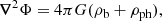
In the AQUAL formulation of MOND, Eq. (1) results from a modification of the gravitational action (or Lagrangian) at a classical level, which also changes the Poisson equation. The AQUAL Poisson equation is
![$$ \begin{aligned} \boldsymbol{\nabla }\left[\mu \left(\dfrac{|\boldsymbol{\nabla }\Phi |}{a_0}\right)\boldsymbol{\nabla }\Phi \right]=4\pi G\rho _{\rm b}, \end{aligned} $$](/articles/aa/full_html/2024/09/aa48211-23/aa48211-23-eq5.gif)
where Φ is the MOND gravitational potential, and ρb is the baryonic matter density. A general solution for the gravitational force arising from the MOND potential can be written as
where S is a curl field, so that ∇ ⋅ S = 0, and gN = −∇ΦN, where ΦN is the Newtonian gravitational potential. Hence, the original formulation of MOND (i.e. Eq. 1) would only be applicable in systems where S vanishes. This has been shown to hold in highly symmetric and/or one-dimensional systems, that is, when |∇ΦN|=f(ΦN) can be written for some smooth function f. An important example for which this holds are flattened systems in which the isopotential surfaces are locally spherically symmetric, such as Kuzmin disks and disk-plus-bulge generalisations thereof (Brada & Milgrom 1995). For a Kuzmin disk of mass M, it can be shown that  .
.
3.1. Milky Way models
To derive a Milky Way potential in the MOND framework, and hence, the force field necessary to integrate the orbits of the Helmi streams stars, we focused on the baryonic components of our Galaxy, namely its disk and bulge. For simplicity, we used the descriptions of these components from two widely employed models that we describe below. In this way, we extended the pioneering work of Read & Moore (2005) by using potentials more complex than the Kuzmin disk. We note that Brada & Milgrom (1995) showed for disk rotation curves that the original approximation given by Eq. (1) holds beyond R = 5 kpc in Kuzmin and exponential disks, and that this equation provides a good approximation to the rotation curves for bulge plus disk potentials (Milgrom 1986). This means that we can use the constraint of the circular velocity at R⊙ = 8.2 kpc to fit our MOND models.
We first focused on the McMillan model (McM model), which stems from the baryonic component from McMillan (2017). In order to match the measured circular velocity at the position of the Sun, we needed to slightly increase the surface mass density of the thin-disk component by 10% from Σd = 9 × 10⁸ M⊙ to 1 × 10⁹ M⊙. The rotation curve provided by this model is shown in the left panel of Fig. 2 and is compared to the original Newtonian McM model. We modified the dark matter halo of the latter model to have qρ = 1.2, following D22. This does not affect the rotation curve in the disk plane, however.
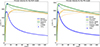 |
Fig. 2. Rotation curves for the McM model (left panel) and the PW model (right panel). The solid lines show the components for the Newtonian framework. All dashed lines correspond to the MOND framework. The horizontal dotted black line shows the MONDian asymptotic velocity of the velocity curve, |
![$ v_{\mathrm{f}}=\sqrt[4]{GM_{\mathrm{bary}}a_0} $](/articles/aa/full_html/2024/09/aa48211-23/aa48211-23-eq8.gif)
We also explored the Price-Whelan model (PW model), which consists of a disk and a bulge, adapted from the baryonic component of the MilkyWayPotential in gala v1.4 (Price-Whelan 2017; Price-Whelan et al. 2021), building on the disk model from Bovy (2015). The disk has a Miyamoto-Nagai potential (Miyamoto & Nagai 1975),
with  , Md = 7.5 × 10¹⁰ M⊙, aMN = 3 kpc, and bMN = 280 pc. We again increased the mass of the disk in this model from its default value by ∼15%. The bulge has a potential following a Hernquist (1990) profile,

with  , Mb = 5 × 10⁹ M⊙, and aH = 1 kpc.
In Newtonian gravity, the default Price-Whelan model has a dark matter halo that follows a flattened NFW potential (Navarro et al. 1997),

where 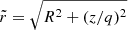 , q = 0.95 is the flattening in the z-direction, Mh = 7 × 10¹¹ M⊙ is the halo mass, and ra = 15.62 kpc is the scale radius.
The left panel of Fig. 2 shows the rotation curves of the McM model in both the Newtonian (i.e. including the dark matter halo, solid) and MOND (dashed) frameworks. We calculated circular velocities as  in the disk plane z = 0, where we used Eq. (11) for the MOND forces.
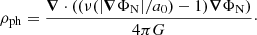
The right panel shows the results for the PW model, where we also show the contribution from the phantom dark matter density. This phantom dark matter density is the effective density of dark matter that would have caused the MOND force field in Newtonian gravity, that is,
where ρb is the baryonic density, and ρph is the phantom dark matter density. Therefore, if the Newtonian potential is known, we can directly infer the functional form of the phantom dark matter density,
Here,
is a function such that we can write
which in terms of Eq. (1) means that ν(y) = 1/μ(x), where y = xμ(x) for S = 0 (Famaey & McGaugh 2012).
Figure 3 compares the density of the PW model in the x − z-plane for the Newtonian (bottom row) and MOND (top row) frameworks. The contours reveal that the phantom dark matter follows the shape of the disk at low heights above the plane, but is spherically symmetric farther away.
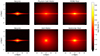 |
Fig. 3. Density profiles of the baryonic [left column], (phantom) dark matter [middle column], and total density for the PW model, showing that the phantom dark matter is constrained to follow the shape of the disk baryonic distribution. |
3.2. External field effect
An important characteristic of MOND due to its non-locality is that the external field acting on a system can have a significant effect (see e.g. Milgrom 1983a, 2010; Banik & Zhao 2018). When we studied the individual orbits of Helmi streams stars in the Milky Way, this external field effect (EFE) could arise from the presence of dwarf galaxies such as Sagittarius (Sgr) or the Large Magellanic Cloud (LMC), or it might be caused by Andromeda (M 31), the largest galaxy closest to the Milky Way. To study the importance of accounting for the EFE due to these objects, we calculated where an external field produces a force equal to the internal field of the Milky Way. This occurs at a radius of
where Mbary, MW is the total baryonic mass of the Milky Way in the MOND framework, and gext is the MOND gravitational acceleration due to the external object. For an object with a total baryonic mass Mbary and a radius r, the rotational velocity flattens at a plateau with a final velocity ![$ v_{\mathrm{f}} = \sqrt[4]{GM_{\mathrm{bary}}a_0} $](/articles/aa/full_html/2024/09/aa48211-23/aa48211-23-eq21.gif) , so that the MOND gravitational acceleration felt at a distance d ≫ r from such an object is
, so that the MOND gravitational acceleration felt at a distance d ≫ r from such an object is  .
.
For M 31, vf ≈ 225 km s−1 (Carignan et al. 2006) and d ≈ 770 kpc, so that gext = 0.02a0, which is well within the deep-MOND limit. Therefore, REFE ∼ 450 − 490 kpc for the external field effect from Andromeda on the Milky Way for the McM and PW models. In our orbit integrations, Helmi streams stars reach an apocenter of 21 kpc, which is much smaller than REFE, and hence, the orbits should not be affected significantly by the external field effect due to M 31 (Banik et al. 2020). Additionally, it has been shown Zhao et al. (2013) that M 31 has remained farther away than 600 kpc from the Milky Way in the past ∼8 Gyr, meaning that the Helmi streams have been orbiting the Galaxy without considerable influence from M 31 since their accretion, which has been estimated to have taken place 5−8 Gyr ago (Koppelman et al. 2019). This conclusion was supported by Oria et al. (2021), who reported that the external field effect of M 31 and also that of the Virgo cluster can be neglected (for objects orbiting) in the inner regions of the Milky Way.
For the LMC and Sgr, we find based on a similar argument that their influence evolves over time while they orbit the MW, and that they enter regimes where their influence on the Helmi streams stars is not negligible (see also Brada & Milgrom 2000). Therefore, we chose to run additional tests in which we included Sgr or the LMC while integrating the Helmi streams stars orbits. To this end, we modelled both Sgr and the LMC using Hernquist spherical potentials with MSgr = 1 × 10⁸ M⊙, aH, Sgr = 0.5 kpc (Vasiliev & Belokurov 2020; McConnachie 2012), and MLMC = 3.2 × 10⁹ M⊙, aH, LMC = 2 kpc (Besla 2015), where their masses correspond to the estimates of their baryonic content.
3.3. Simplified orbit integrations
As a first step to investigate the Helmi streams in MOND, we performed orbit integrations in the MOND framework, simplified by omitting the influence of the curl field S, and we compared these with orbits integrated in the original McM and PW Milky Way models that include dark matter haloes and use Newtonian gravity. We note that we can only safely omit the curl field S from our analysis and use gMOND = ν(|gN|/a0)gN when the relation  can be used, where Mb is the baryonic mass of the model (Brada & Milgrom 1995; Milgrom 1986). Close to the disk, where |z|< 1.5 kpc (2.5 kpc for the McM model) and within R ≲ 30 kpc, the above relation does not hold. The LMC does not pass this region on its orbit, and therefore, we can use Eq. (11) to integrate its orbit. Sgr has a pericenter of ∼20 kpc, and the stars in our Helmi streams sample are currently located within 2.5 kpc from the Sun. Still, for most of the time, the orbits of Sgr and the Helmi streams are in a region in which our simplification holds. Reassuringly, in Section 4, where we explore the behaviour of the Helmi streams using PoR, we show that their orbits are barely affected by our simplification. The validity of this approach for the orbit integrations outside of the disk area does not change when we add Sgr and the LMC to the MOND Milky Way potential. Their contribution is both small and locally spherically symmetric, so that S can still be neglected because
  holds in the region of the Helmi streams at each time in the presence of either Sgr or the LMC.
To compute the orbit of a star from the Helmi streams, we used its present-day position and velocity and integrated the equation of motion backward in time using the MOND force associated with the Milky Way potential under consideration. We used a leapfrog integrator, with a time step of Δt = 0.2 Myr. For the Newtonian models, we used the integrator implemented in AGAMA with the same time step.
To include either of the Milky Way satellites, namely Sgr or the LMC, we first determined their orbit in the MOND Milky Way model without the Helmi streams stars. Then, we used the appropriate Hernquist potential representing the baryonic component of the satellite at the position of the satellite through time as an addition to the background potential in which we integrated our Helmi streams stars. Figure 4 shows the orbit of one of the Helmi streams stars in the PW model. For comparison, we also plot the orbit obtained including Sgr, as well as that using Newtonian gravity. This figure shows that the presence of Sgr does not lead to significant differences in the trajectory of the Helmi streams stars, but that there are important differences between the MOND and Newtonian frameworks.
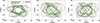 |
Fig. 4. Orbit of one of the Helmi streams stars in the Newtonian potential (solid, green), the MOND potential (solid, blue), and the MOND potential including Sgr (dotted, orange) for the PW model. The dot shows the initial position of all three orbits. |
Figures 5 and 6 show the behaviour of the Helmi streams stars in the Lz − L⊥ plane stemming from our simplified orbit integrations for the McM and PW models, respectively. In Fig. 5, the top row corresponds to the Newtonian model, the second row shows the corresponding MOND model, and the bottom two rows include Sgr and the LMC. The columns show four snapshots through the time of integration, at 0, 0.1, 2 and 4 Gyr. Because the results were similar to those for the McM model when we added Sgr and LMC to the PW model, we do not show them again in Fig. 6.
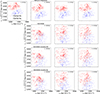 |
Fig. 5. Evolution of the Helmi streams stars in Lz − L⊥ over time in the McM Newtonian model of the Milky Way (with a modified dark matter halo with a flattening of q = 1.2, as favoured by D22, in the top row), the MOND version of this potential (second row) and the MOND versions including the effect of Sgr (third row) and of the LMC (bottom row). The first column shows the present-day observed distribution, the second column shows the distribution after ∼100 Myr, and the third and fourth columns show the distribution after ∼2 and ∼4 Gyr of integration, respectively. |
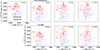 |
Fig. 6. Same as Fig. 5, but for the PW model, where the top row shows the results for the Newtonian PW potential (which has a flattening of q = 0.95). |
Clearly, the gap between the two Helmi streams clumps does not persist in the MOND models, regardless of whether Sgr or the LMC is included, which does not change the orbital behaviour visibly. The result is also valid regardless of the choice of baryonic potential for the Milky Way.
The two clumps mix significantly already within the first ∼100 Myr in all MOND models, with blue and red stars changing their L⊥ strongly enough for a distinction between the two groups to be no longer possible. This extremely fast mixing behaviour is not seen for the Newtonian PW model, which has an oblate dark matter halo with a flattening of q = 0.95. However, in this Newtonian model, the gap does not persist over long timescales either, as it disappears after ∼200 Myr, although the degree and rate by which the stars in the red and blue clumps are mixing is lower than the MOND models. In the Newtonian McM model with qρ = 1.2, there is no mixing by construction (see D22 for details).
4. Phantom of RAMSES
We also calculated the orbits of the Helmi streams stars in the McM model using the phantom of RAMSES (PoR) patch to the RAMSES N-body code to provide insight into a more sophisticated MOND framework (Lüghausen et al. 2015; Teyssier 2010).
We note that the PoR patch is based on the QUMOND formulation of MOND, whereas our orbit integrations and discussion of the S field were based on the AQUAL formulation of MOND. Hence, the results between the two frameworks do not necessarily agree (Milgrom 2010; Famaey & McGaugh 2012). We employed the staticpart flag to represent the baryonic components of the McM model with a collection of particles that continually generated the MONDian gravitational potential in which the Helmi streams stars were integrated. We generated the positions of these static particles using AGAMA (Vasiliev 2019) to represent the baryonic density profiles. We integrated the orbits of the Helmi streams stars for 2 Gyr using a minimum and maximum grid level of 7 and 18, respectively. This is sufficiently precise to model the orbit well. The box size of the simulation was 1024 kpc, ensuring that the potential can be approximated by a point source at the boundary of the box.
The top row of Figure 7 shows the orbit of one of the Helmi streams stars in the PoR simulation compared to its orbit in the simplified orbit integration from Section 3. Even though there is a difference that builds up over this time, the nature of the orbit is not altered. The bottom row shows the Lz − L⊥ plane for the Helmi streams particles in the PoR simulation at time stamps of t = 0, 0.1 and 2 Gyr. Again, the gap between the two Helmi streams clumps dissolves within 100 Myr, although the degree of mixing of the stars in the two clumps is lower than in the simplified orbit integrations shown in the second row of Fig. 5. After 2 Gyr, however, the two clumps show a similar degree of mixing in both the PoR and simplified orbit integrations.
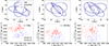 |
Fig. 7. Results from the phantom of RAMSES simulations. Top row: Three projections of the orbit of one of the Helmi streams stars in the simplified MOND orbit integrations from Sect. 3 (solid, blue) and in phantom of RAMSES (dashed, black). The dot shows the initial position. Bottom row: Lz − L⊥ plane for the Helmi streams stars in the PoR simulation at time stamps of (left to right) 0, 0.1, and 2 Gyr. |
We may therefore conclude from Figs. 5, 6 and 7 that the simplified modelling as well as the sophisticated PoR integrations of the Milky Way in MOND employed here fail to reproduce the observations of the Helmi streams. Whether this is indicative of a shortcoming of our implementation of MOND or if this means that the MOND theory, perhaps as a modification of inertia, should be altered, remains to be determined.
5. Discussion and conclusion
We have shown by way of simplified orbit integrations in MOND models of the Milky Way using AQUAL as well as orbit integrations in QUMOND using the PoR patch for RAMSES that the gap between the two observed clumps in Lz − L⊥ space for the Helmi streams does not persist through time. The stars in the clumps intermix very quickly, namely already in the first ∼100 Myr of integration, as shown in Figs. 5, 6 and 7. This leads to the dissolution of the gap and to the mixing of the clumps. When we take our implementation of MOND at face value, this places us in the uncomfortable position of having to argue that we are living at a truly special time in Galactic history.
A question that may naturally arise is whether the presence of two separate clumps might reflect some internal substructure that existed in the progenitor system. In that case, the question is whether the gap between the clumps was initially larger, such that it could have developed to its currently observed form after a few billion years of evolution in the Milky Way (although this may even be challenging for the MOND models). There is a fundamental problem with this argument, however. By definition, substructure is localised in phase space in a (progenitor) system. As the system is accreted, phase space folds, leading to the presence of multiple streams. Each of the streams stems from a (very) small region of the original system (particularly if phase-mixing has occurred as is the case for the Helmi streams, Helmi et al. 1999). Therefore, substructure in the progenitor system should be apparent in a localised portion of a stream. Fig. 1 shows that multiple kinematic streams (e.g. with positive and negative vz) are associated with each of the two clumps in angular momentum space. This indicates that the clumps cannot be the result a local feature or substructure in the progenitor system because the stars in a given clump stem from a large region of phase space of this system.
Our results can be compared to Figs. 8 and 9 of D22, who have shown that for the clumps to be distinguishable over long timescales, a prolate halo with a density flattening qρ ∼ 1.2 would seem to be necessary, as we have exemplified in the top panels of Fig. 5. This renders the effective potential to be close to spherical somewhere in the region probed by the stream stars, which results in a better conservation of L⊥, and hence, of the clump individuality. A prolate shape for the dark matter halo like this cannot be naturally produced in a MOND framework because the gravitational field is constrained to follow the shape of the baryonic distribution, which is highly oblate (see Fig. 3). The failure of our MONDian orbit integrations to reproduce the observed properties of the streams is thus not so surprising.
We expect our conclusions to be robust because we showed here that the dissolution of the gap between the clumps occurs both in AQUAL with simplified orbit integrations either with or without the influence of the two largest satellites of the Milky Way and also in the QUMOND framework, which was studied through the PoR patch for RAMSES. We also ran our integrations using a Kuzmin model for the Milky Way potential, as in Read & Moore (2005), where S = 0 holds strictly, and the results were not different from those presented here.
Nonetheless, it would be important to explore other possible formulations of MOND, and specifically, as a modification of inertia, which unfortunately is not yet completely developed. Complications arising in this framework are, for instance, the non-locality in time and the fact that the definition of actions and conserved quantities such as momentum could be different from the Newtonian definitions (Milgrom 2006, 2022).
The observations of the Helmi streams clumps provide a particularly good test for MOND on Galactic scales because the stars probe a region that is mainly governed by the gravitational field of the Galaxy. Furthermore, their orbits are elongated in the direction perpendicular to the Galactic disk, a regime that has not been explored much in the context of MOND. As discussed in Zhu et al. (2023), for example, MOND and Newtonian gravity including a dark matter halo are able to fit the Galaxy rotation curve equally well. There is thus a need for more studies like ours that probe a larger distance from the disk plane. An interesting example is the proposal to use high-velocity stars, as these objects probe regions where the two theories would predict a rather different behaviour (Chakrabarty et al. 2022).
Acknowledgments
We thank Bob Sanders (and indirectly M. Milgrom) for sharing his knowledge on MOND and very useful discussions. We are also grateful to the referee for their very constructive report. We acknowledge financial support from a Spinoza prize. We have made use of data from the European Space Agency (ESA) mission Gaia (https://www.cosmos.esa.int/gaia), processed by the Gaia Data Processing and Analysis Consortium (DPAC, https://www.cosmos.esa.int/web/gaia/dpac/consortium). Funding for the DPAC has been provided by national institutions, in particular the institutions participating in the Gaia Multilateral Agreement. Throughout this work, we have made use of the following packages: astropy (Astropy Collaboration 2013), vaex (Breddels & Veljanoski 2018), SciPy (Virtanen et al. 2020), matplotlib (Hunter 2007), NumPy (van der Walt et al. 2011), AGAMA (Vasiliev 2019) and Jupyter Notebooks (Kluyver et al. 2016).
References
- Ahumada, R., Allende Prieto, C., Almeida, A., et al. 2020, ApJS, 249, 3 [NASA ADS] [CrossRef] [Google Scholar]
- Astropy Collaboration (Robitaille, T. P., et al.) 2013, A&A, 558, A33 [NASA ADS] [CrossRef] [EDP Sciences] [Google Scholar]
- Banik, I., & Zhao, H. 2018, MNRAS, 473, 419 [NASA ADS] [CrossRef] [Google Scholar]
- Banik, I., & Zhao, H. 2022, Symmetry, 14, 1331 [NASA ADS] [CrossRef] [Google Scholar]
- Banik, I., Thies, I., Famaey, B., et al. 2020, ApJ, 905, 135 [Google Scholar]
- Bekenstein, J., & Milgrom, M. 1984, ApJ, 286, 7 [NASA ADS] [CrossRef] [Google Scholar]
- Besla, G. 2015, ArXiv e-prints [arXiv:1511.03346] [Google Scholar]
- Binney, J., Gerhard, O., & Spergel, D. 1997, MNRAS, 288, 365 [NASA ADS] [CrossRef] [Google Scholar]
- Bosma, A. 1981, ApJ, 86, 1825 [Google Scholar]
- Bovy, J. 2015, ApJS, 216, 29 [NASA ADS] [CrossRef] [Google Scholar]
- Boylan-Kolchin, M., Bullock, J. S., & Kaplinghat, M. 2011, MNRAS, 415, L40 [NASA ADS] [CrossRef] [Google Scholar]
- Brada, R., & Milgrom, M. 1995, MNRAS, 276, 453 [Google Scholar]
- Brada, R., & Milgrom, M. 2000, ApJ, 541, 556 [NASA ADS] [CrossRef] [Google Scholar]
- Breddels, M. A., & Veljanoski, J. 2018, A&A, 618, A13 [NASA ADS] [CrossRef] [EDP Sciences] [Google Scholar]
- Buder, S., Sharma, S., Kos, J., et al. 2021, MNRAS, 506, 150 [NASA ADS] [CrossRef] [Google Scholar]
- Bullock, J. S., & Boylan-Kolchin, M. 2017, ARA&A, 55, 343 [Google Scholar]
- Carignan, C., Chemin, L., Huchtmeier, W. K., & Lockman, F. J. 2006, ApJ, 641, L109 [NASA ADS] [CrossRef] [Google Scholar]
- Chakrabarty, S. S., Ostorero, L., Gallo, A., Ebagezio, S., & Diaferio, A. 2022, A&A, 657, A115 [NASA ADS] [CrossRef] [EDP Sciences] [Google Scholar]
- Cui, X.-Q., Zhao, Y.-H., Chu, Y.-Q., et al. 2012, RAA, 12, 1197 [NASA ADS] [Google Scholar]
- Dai, D.-C., Starkman, G., & Stojkovic, D. 2022, Phys. Rev. D, 105, 104067 [CrossRef] [Google Scholar]
- Dehnen, W., Odenkirchen, M., Grebel, E. K., & Rix, H.-W. 2004, AJ, 127, 2753 [NASA ADS] [CrossRef] [Google Scholar]
- Dodd, E., Helmi, A., & Koppelman, H. H. 2022, A&A, 659, A61 [NASA ADS] [CrossRef] [EDP Sciences] [Google Scholar]
- Dodd, E., Callingham, T. M., Helmi, A., et al. 2023, A&A, 670, L2 [NASA ADS] [CrossRef] [EDP Sciences] [Google Scholar]
- Erkal, D., & Belokurov, V. 2015, MNRAS, 450, 1136 [Google Scholar]
- Famaey, B., & Binney, J. 2005, MNRAS, 363, 603 [NASA ADS] [CrossRef] [Google Scholar]
- Famaey, B., & McGaugh, S. S. 2012, Liv. Rev. Relat., 15, 10 [Google Scholar]
- Finan-Jenkin, M., & Easther, R. 2023, ArXiv e-prints [arXiv:2306.15939] [Google Scholar]
- Gaia Collaboration (Prusti, T., et al.) 2016, A&A, 595, A1 [NASA ADS] [CrossRef] [EDP Sciences] [Google Scholar]
- Gaia Collaboration (Klioner, S. A., et al.) 2021a, A&A, 649, A9 [EDP Sciences] [Google Scholar]
- Gaia Collaboration (Brown, A. G. A., et al.) 2021b, A&A, 649, A1 [NASA ADS] [CrossRef] [EDP Sciences] [Google Scholar]
- Garavito-Camargo, N., Price-Whelan, A. M., Samuel, J., et al. 2023, ArXiv e-prints [arXiv:2311.11359] [Google Scholar]
- Helmi, A., & de Zeeuw, P. T. 2000, MNRAS, 319, 657 [Google Scholar]
- Helmi, A., White, S. D. M., de Zeeuw, P. T., & Zhao, H. 1999, Nature, 402, 53 [Google Scholar]
- Hernquist, L. 1990, ApJ, 356, 359 [Google Scholar]
- Hunter, J. D. 2007, Comput. Sci. Eng., 9, 90 [NASA ADS] [CrossRef] [Google Scholar]
- Ibata, R. A., Lewis, G. F., Irwin, M. J., & Quinn, T. 2002, MNRAS, 332, 915 [Google Scholar]
- Johnston, K. V., Spergel, D. N., & Haydn, C. 2002, ApJ, 570, 656 [NASA ADS] [CrossRef] [Google Scholar]
- Kluyver, T., Ragan-Kelley, B., Pérez, F., et al. 2016, in Positioning and Power in Academic Publishing: Players, Agents and Agendas, eds. F. Loizides, & B. Scmidt (IOS Press) [Google Scholar]
- Koppelman, H. H., Helmi, A., Massari, D., Roelenga, S., & Bastian, U. 2019, A&A, 625, A5 [NASA ADS] [CrossRef] [EDP Sciences] [Google Scholar]
- Kroupa, P., Jerabkova, T., Thies, I., et al. 2022, MNRAS, 517, 3613 [CrossRef] [Google Scholar]
- Lelli, F., McGaugh, S. S., & Schombert, J. M. 2016, ApJ, 816, L14 [Google Scholar]
- Libeskind, N. I., Frenk, C. S., Cole, S., et al. 2005, MNRAS, 363, 146 [NASA ADS] [CrossRef] [Google Scholar]
- Lindegren, L., Klioner, S. A., Hernández, J., et al. 2021, A&A, 649, A2 [EDP Sciences] [Google Scholar]
- Lisanti, M., Moschella, M., Outmezguine, N. J., & Slone, O. 2019, Phys. Rev. D, 100, 083009 [NASA ADS] [CrossRef] [Google Scholar]
- Lövdal, S. S., Ruiz-Lara, T., Koppelman, H. H., et al. 2022, A&A, 665, A57 [NASA ADS] [CrossRef] [EDP Sciences] [Google Scholar]
- Lüghausen, F., Famaey, B., & Kroupa, P. 2015, Can. J. Phys., 93, 232 [CrossRef] [Google Scholar]
- McConnachie, A. W. 2012, AJ, 144, 4 [Google Scholar]
- McGaugh, S. S., Lelli, F., & Schombert, J. M. 2016, Phys. Rev. Lett., 117, 201101 [NASA ADS] [CrossRef] [Google Scholar]
- McMillan, P. J. 2017, MNRAS, 465, 76 [NASA ADS] [CrossRef] [Google Scholar]
- Milgrom, M. 1983a, ApJ, 270, 371 [Google Scholar]
- Milgrom, M. 1983b, ApJ, 270, 384 [Google Scholar]
- Milgrom, M. 1986, ApJ, 302, 617 [NASA ADS] [CrossRef] [Google Scholar]
- Milgrom, M. 2006, EAS Publ. Ser., 20, 217 [NASA ADS] [CrossRef] [EDP Sciences] [Google Scholar]
- Milgrom, M. 2010, MNRAS, 403, 886 [NASA ADS] [CrossRef] [Google Scholar]
- Milgrom, M. 2022, Phys. Rev. D, 106, 064060 [NASA ADS] [CrossRef] [Google Scholar]
- Miyamoto, M., & Nagai, R. 1975, PASJ, 27, 533 [NASA ADS] [Google Scholar]
- Navarro, J. F., Frenk, C. S., & White, S. D. M. 1997, ApJ, 490, 493 [Google Scholar]
- Oort, J. H. 1932, Bull. Astron. Inst. Neth., 6, 249 [NASA ADS] [Google Scholar]
- Oria, P. A., Famaey, B., Thomas, G. F., et al. 2021, ApJ, 923, 68 [NASA ADS] [CrossRef] [Google Scholar]
- Ostriker, J. P., & Peebles, P. J. E. 1973, ApJ, 186, 467 [Google Scholar]
- Pawlowski, M. S., Ibata, R. A., & Bullock, J. S. 2017, ApJ, 850, 132 [NASA ADS] [CrossRef] [Google Scholar]
- Pearson, S., Price-Whelan, A. M., & Johnston, K. V. 2017, Nat. Astron., 1, 633 [NASA ADS] [CrossRef] [Google Scholar]
- Price-Whelan, A. M. 2017, J. Open Source Softw., 2, 388 [NASA ADS] [CrossRef] [Google Scholar]
- Price-Whelan, A., Sipőcz, B., Starkman, N., et al. 2021, https://doi.org/10.5281/zenodo.5057630 [Google Scholar]
- Read, J. I., & Moore, B. 2005, MNRAS, 361, 971 [NASA ADS] [CrossRef] [Google Scholar]
- Rubin, V. C., Ford, W. K., Thonnard, N., & Burstein, D. 1982, ApJ, 261, 439 [NASA ADS] [CrossRef] [Google Scholar]
- Ruiz-Lara, T., Matsuno, T., Lövdal, S. S., et al. 2022, A&A, 665, A58 [NASA ADS] [CrossRef] [EDP Sciences] [Google Scholar]
- Sales, L. V., Wetzel, A., & Fattahi, A. 2022, Nat. Astron., 6, 897 [NASA ADS] [CrossRef] [Google Scholar]
- Sanders, R. H. 1999, ApJ, 512, L23 [NASA ADS] [CrossRef] [Google Scholar]
- Sawala, T., Cautun, M., Frenk, C., et al. 2023, Nat. Astron., 7, 481 [Google Scholar]
- Schönrich, R., Binney, J., & Dehnen, W. 2010, MNRAS, 403, 1829 [CrossRef] [Google Scholar]
- Skordis, C., & Złośnik, T. 2021, Phys. Rev. Lett., 127, 161302 [NASA ADS] [CrossRef] [Google Scholar]
- Steinmetz, M., Matijevič, G., Enke, H., et al. 2020, AJ, 160, 82 [NASA ADS] [CrossRef] [Google Scholar]
- Sylos Labini, F., Chrobáková, Ž., Capuzzo-Dolcetta, R., & López-Corredoira, M. 2023, ApJ, 945, 3 [NASA ADS] [CrossRef] [Google Scholar]
- Teyssier, R. 2010, Astrophysics Source Code Library [record ascl:1011.007] [Google Scholar]
- Thomas, G. F., Famaey, B., Ibata, R., Lüghausen, F., & Kroupa, P. 2017, A&A, 603, A65 [NASA ADS] [CrossRef] [EDP Sciences] [Google Scholar]
- Thomas, G. F., Famaey, B., Ibata, R., et al. 2018, A&A, 609, A44 [NASA ADS] [CrossRef] [EDP Sciences] [Google Scholar]
- van der Walt, S., Colbert, S. C., & Varoquaux, G. 2011, Comput. Sci. Eng., 13, 22 [Google Scholar]
- Vasiliev, E. 2019, MNRAS, 482, 1525 [Google Scholar]
- Vasiliev, E., & Belokurov, V. 2020, MNRAS, 497, 4162 [Google Scholar]
- Virtanen, P., Gommers, R., Oliphant, T. E., et al. 2020, Nat. Meth., 17, 261 [Google Scholar]
- Zhao, H., Famaey, B., Lüghausen, F., & Kroupa, P. 2013, A&A, 557, L3 [NASA ADS] [CrossRef] [EDP Sciences] [Google Scholar]
- Zhu, Y., Ma, H.-X., Dong, X.-B., et al. 2023, MNRAS, 519, 4479 [NASA ADS] [CrossRef] [Google Scholar]
- Zwicky, F. 1933, Helv. Phys. Acta, 6, 110 [NASA ADS] [Google Scholar]
All Figures
|
Fig. 1. Helmi streams stars within 2.5 kpc as selected by D22 shown in colour in velocity space (top panels) and Lz − L⊥ space (bottom left panel and zoom-in on the right). The grey dots and contours show the full Gaia sample within 2.5 kpc. The darker coloured squares are all Helmi streams stars with Gaia radial velocities, and the lighter coloured dots show stars with ground-based radial velocities. While the Helmi streams stars are visibly clumped in vz − vy space, the streams are clearly distributed into two distinct clumps in Lz − L⊥ space. One clump has high L⊥ (hiL, red), and the other clump has low L⊥ (loL, blue). |
| In the text | |
|
Fig. 2. Rotation curves for the McM model (left panel) and the PW model (right panel). The solid lines show the components for the Newtonian framework. All dashed lines correspond to the MOND framework. The horizontal dotted black line shows the MONDian asymptotic velocity of the velocity curve, |
| In the text | |
|
Fig. 3. Density profiles of the baryonic [left column], (phantom) dark matter [middle column], and total density for the PW model, showing that the phantom dark matter is constrained to follow the shape of the disk baryonic distribution. |
| In the text | |
|
Fig. 4. Orbit of one of the Helmi streams stars in the Newtonian potential (solid, green), the MOND potential (solid, blue), and the MOND potential including Sgr (dotted, orange) for the PW model. The dot shows the initial position of all three orbits. |
| In the text | |
|
Fig. 5. Evolution of the Helmi streams stars in Lz − L⊥ over time in the McM Newtonian model of the Milky Way (with a modified dark matter halo with a flattening of q = 1.2, as favoured by D22, in the top row), the MOND version of this potential (second row) and the MOND versions including the effect of Sgr (third row) and of the LMC (bottom row). The first column shows the present-day observed distribution, the second column shows the distribution after ∼100 Myr, and the third and fourth columns show the distribution after ∼2 and ∼4 Gyr of integration, respectively. |
| In the text | |
|
Fig. 6. Same as Fig. 5, but for the PW model, where the top row shows the results for the Newtonian PW potential (which has a flattening of q = 0.95). |
| In the text | |
|
Fig. 7. Results from the phantom of RAMSES simulations. Top row: Three projections of the orbit of one of the Helmi streams stars in the simplified MOND orbit integrations from Sect. 3 (solid, blue) and in phantom of RAMSES (dashed, black). The dot shows the initial position. Bottom row: Lz − L⊥ plane for the Helmi streams stars in the PoR simulation at time stamps of (left to right) 0, 0.1, and 2 Gyr. |
| In the text | |
Current usage metrics show cumulative count of Article Views (full-text article views including HTML views, PDF and ePub downloads, according to the available data) and Abstracts Views on Vision4Press platform.
Data correspond to usage on the plateform after 2015. The current usage metrics is available 48-96 hours after online publication and is updated daily on week days.
Initial download of the metrics may take a while.