| Issue |
A&A
Volume 592, August 2016
|
|
|---|---|---|
| Article Number | A131 | |
| Number of page(s) | 13 | |
| Section | Interstellar and circumstellar matter | |
| DOI | https://doi.org/10.1051/0004-6361/201527290 | |
| Published online | 12 August 2016 | |
Herschel/HIFI observations of the circumstellar ammonia lines in IRC+10216 ⋆,⋆⋆
1 N. Copernicus Astronomical Center,
Rabiańska 8, 87-100 Toruń, Poland
e-mail: This email address is being protected from spambots. You need JavaScript enabled to view it.
2 Key Laboratory for the Structure and
Evolution of Celestial Objects, Yunnan Observatories, Chinese Academy of Sciences,
PO Box 110,
Kunming, Yunnan
Province, PR China
3 Observatorio Astronómico Nacional. Ap
112, 28803
Alcalá de Henares,
Spain
4 Observatorio Astronómico Nacional
(IGN), Alfonso XII
N ◦ 3,
28014
Madrid,
Spain
5 ICMM, CSIC, group of Molecular
Astrophysics, C/Sor Juana Inés de la Cruz N3, 28049 Cantoblanco,
Madrid,
Spain
6 Instituut voor Sterrenkunde,
Katholieke Universiteit Leuven, Celestijnenlaan 200D, 3001
Leuven,
Belgium
7 Sterrenkundig Instituut Anton
Pannekoek, University of Amsterdam, Science Park 904, 1098
Amsterdam, The
Netherlands
8 Chalmers University of Technology,
Department of Earth and Space Sciences, Onsala Space Observatory,
439 92
Onsala,
Sweden
9 European Space Astronomy Centre, ESA,
PO Box 78, 28691 Villanueva de la Cañada, Madrid, Spain
10 Max-Planck-Institut für
Radioastronomie, Auf dem Hügel
69, 53121
Bonn,
Germany
11 Johns Hopkins Universtity,
Baltimore,
MD
21218,
USA
12 Department of Astronomy, AlbaNova
University Center, Stockholm University, 10691
Stockholm,
Sweden
13 Ural Federal University,
Astronomical Observatory, 620000
Ekaterinburg, Russian
Federation
Received:
1
September
2015
Accepted:
23
May
2016
Abstract
Context. A discrepancy exists between the abundance of ammonia (NH3) derived previously for the circumstellar envelope (CSE) of IRC+10216 from far-IR submillimeter rotational lines and that inferred from radio inversion or mid-infrared (MIR) absorption transitions.
Aims. To address the discrepancy described above, new high-resolution far-infrared (FIR) observations of both ortho- and para-NH3 transitions toward IRC+10216 were obtained with Herschel, with the goal of determining the ammonia abundance and constraining the distribution of NH3 in the envelope of IRC+10216.
Methods. We used the Heterodyne Instrument for the Far Infrared (HIFI) on board Herschel to observe all rotational transitions up to the J = 3 level (three ortho- and six para-NH3 lines). We conducted non-LTE multilevel radiative transfer modelling, including the effects of near-infrared (NIR) radiative pumping through vibrational transitions. The computed emission line profiles are compared with the new HIFI data, the radio inversion transitions, and the MIR absorption lines in the ν2 band taken from the literature.
Results. We found that NIR pumping is of key importance for understanding the excitation of rotational levels of NH3. The derived NH3 abundances relative to molecular hydrogen were (2.8 ± 0.5) × 10-8 for ortho-NH3 and (3.2 -0.6+0.7) × 10 -8 for para-NH3, consistent with an ortho/para ratio of 1. These values are in a rough agreement with abundances derived from the inversion transitions, as well as with the total abundance of NH3 inferred from the MIR absorption lines. To explain the observed rotational transitions, ammonia must be formed near to the central star at a radius close to the end of the wind acceleration region, but no larger than about 20 stellar radii (1σ confidence level).
Key words: stars: AGB and post-AGB / circumstellar matter / stars: carbon / stars: individual: IRC+10216
Herschel is an ESA space observatory with science instruments provided by European-led Principal Investigator consortia and with important participation from NASA. HIFI is the Herschel Heterodyne Instrument for the Far Infrared.
The reduced spectra (FITS files) are only available at the CDS via anonymous ftp to cdsarc.u-strasbg.fr (130.79.128.5) or via http://cdsarc.u-strasbg.fr/viz-bin/qcat?J/A+A/592/A131
Deceased 14 January 2011.
© ESO, 2016
1. Introduction
Ammonia (NH3) was the first polyatomic molecule discovered in space (Cheung et al. 1968), and has subsequently been one of the most extensively observed molecules in the interstellar medium (Ho & Townes 1983), with a set 23 GHz of inversion transitions that are readily detectable from many radio telescopes. Emission lines resulting from these transitions are widely detected in the dense parts of both dark and star-forming molecular clouds (see e.g. Harju et al. 1993; Jijina et al. 1999; Wienen et al. 2012). Because ammonia is a symmetric top molecule, an analysis of its excitation allows the effects of temperature and density to be determined separately; as a result, the metastable lines of ammonia are often used to derive the temperature and density of dense clumps in molecular clouds. (Walmsley & Ungerechts 1983; Danby et al. 1988; Kirsanova et al. 2014).
Ammonia has also been detected in the circumstellar envelopes of evolved stars, but has been observed less extensively in such environments than in the interstellar medium. Several absorption features in the ν2 vibration−rotational bands around 10 μm were detected in some asymptotic giant branch (AGB) stars, as well as in a few massive supergiants (Betz et al. 1979; McLaren & Betz 1980; Betz 1987). At about the same time, the 1.3 cm wavelength inversion transitions of ammonia were detected from C-rich AGB and post-AGB stars (Betz 1987; Nguyen-Q-Rieu et al. 1984, 1986).
In IRC+10216 (CW Leo), ammonia was observed for the first time by its infrared absorption lines in the ν2 band around 10 μm (Betz et al. 1979), and its detection in radio inversion transitions was announced shortly thereafter (Bell et al. 1980). In the following years, new observations of IRC+10216 were performed in both infrared absorption (Keady & Ridgway 1993; Monnier et al. 2000) and radio inversion lines (Kwok et al. 1981; Bell et al. 1982; Nguyen-Q-Rieu et al. 1984; Gong et al. 2015).
IRC+10216 was detected in the Two-micron Sky Survey as the brightest infrared sky object at 5 μm outside the solar system (Becklin et al. 1969), and soon its heavily obscured central star was identified as being C-rich based on the presence of strong CN absorption bands (Herbig & Zappala 1970; Miller 1970). Presently, IRC+10216 is the best studied C-rich AGB star. About half of the molecules detected in space are seen in the envelope of this source, due to its proximity (distance, d, of 130 pc, see Menten et al. 2012) and a relatively large mass loss rate ~1−4 × 10⁻⁵M⊙ yr-1 (e.g. Groenewegen et al. 1998; Truong-Bach et al. 1991).
The development of heterodyne technology for observations in the far-infrared (FIR) enabled the first detection of the 10(s)−00(a) rotational transition of ortho-NH3 by the Odin satellite toward IRC+10216 (Hasegawa et al. 2006), which was followed by the detection of the same transition in some O-rich AGB stars and red-supergiants (Menten et al. 2010) by the Heterodyne Instrument for the Far Infrared (HIFI, de Graauw et al. 2010) on board the Herschel Space Observatory (Herschel, Pilbratt et al. 2010). Furthermore, by fully exploiting the capabilities of the HIFI instrument, we were able to observe all nine rotational transitions up to the J = 3 levels of ortho- and para-NH3 (this paper) in the envelope of IRC+10216.
There is a clear discrepancy between the estimated amount of para-NH3 relative to molecular hydrogen in IRC+10216 derived from radio inversion lines (3 × 10⁻⁸; Kwok et al. 1981) and that of ortho-NH3 derived from its lowest rotational line (about 10-6; Hasegawa et al. 2006). Nevertheless, both values, which lie within the range of ammonia abundances observed towards other C-rich and O-rich stars, and cannot be explained by standard chemical models (see discussion in Menten et al. 2010). However, the chemical model presented recently by Decin et al. (2010) seems able to reproduce the high abundance of ammonia observed in IRC+10216 (see their Fig. 3). Their model, constructed with the aim of explaining the presence of water vapour in the envelope of this C-rich star, assumes a clumpy envelope structure, where a fraction of the interstellar UV photons is able to penetrate deep into the envelope and dissociate mostly 13CO, providing oxygen for O-rich chemistry in the inner warm parts of a C-rich circumstellar envelope. On the other hand, Neufeld et al. (2013) have suggested, on the basis of H2O isotopic ratios, that a recent model invoking shock chemistry (Cherchneff 2012) may provide a more successful explanation for the presence of water in envelopes of C-rich stars. However, this model does not provide information on the ammonia formation.
In this paper we present new Herschel/HIFI observations of nine rotational transitions of NH3 (three ortho and six para lines), eight of which have been detected for the first time, and an analysis of their implications with the use of detailed modelling.
The observations and data reduction are presented in Sect. 2. Section 3 is devoted to the description of the molecular structure of ammonia, while Sect. 4 presents details of the modelling procedure and the best fits found for all rotational transitions. In Sect. 5 we discuss the results thereby obtained and their consequences. Finally, a summary of this study is presented in Sect. 6.
2. Observations
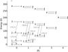 |
Fig. 1 Diagram of energy levels of ortho- (|K| = 0, 3, etc.) and para-NH3 (|K| = 1, 2, 4, etc.). The inversion splitting between levels of different symmetry is exaggerated for clarity. The observed rotational transitions with frequencies in GHz are indicated with arrows. |
Summary of NH3 observations in IRC+10216.
Observations of IRC+10216 were carried out with the Herschel/HIFI instrument as part of the HIFISTARS Guaranteed Time Key Program (Proposal Id: KPGT_vbujarra_1; PI: V. Bujarrabal); in addition, a spectral line survey has been carried out for this object (Proposal Id: GT1_jcernich_4; PI: J. Cernicharo). The observed rotational lines of ortho- and para-NH3 are listed in Table 1 and indicated in Fig. 1, which shows the diagram of the lowest rotational levels of ammonia. For each observed transition, Table 1 gives the line identification, its frequency in GHz, the corresponding HIFI band, the energy of the upper level in K, the Herschel OBServation ID, the date of the observation, the optical phase (φ) of the observation (counted from the reference maximum phase of the light curve, φ = 0, on Julian date JD = 2 454 554 with an assumed period of 630 days (Menten et al. 2012)), the half power beam width (HPBW) of the Herschel telescope at the observed frequency, the main beam efficiency ηmb, the integrated flux in K km s-1 with its estimated uncertainty, and the observing mode: single tuning or spectral scan. In this paper, we analyse wide band spectrometer (WBS) data only.
The HIFI observations of IRC+10216 were reduced with the latest version of HIPE (13.0) with data processed with Standard Product Generator (SPG) version 13.0.0. The data were processed using the HIPE pipeline to level 2, which was set to provide intensities expressed as the main beam temperature. Main beam efficiencies were taken from the recent measurements by Mueller et al. (2014)1. They differ by up to 20% from the older determinations by Roelfsema et al. (2012). Frequencies are always given in the frame of the local standard of rest (LSR).
The statistical uncertainties in the integrated line fluxes, as derived formally from the rms noise in the spectra (see below) are relatively small, while it is known that systematic uncertainties in the HIFI flux calibration are much larger (Roelfsema et al. 2012). Therefore, somewhat arbitrarily, we have assumed a 5% uncertainty in the integrated line flux for lines observed in band 1b, a 10% uncertainty for lines in bands 5a and 7a, and a 50% uncertainty for lines in band 7b. However, since two of the lines observed in band 7a are blended (see below), we increased the assumed uncertainty in their integrated flux from 10 to 15%. The method used to deconvolve line blends and to derive individual line fluxes is described in Sect. 2.2. The observed line profiles are shown by the solid lines in Fig. 2.
2.1. Single point observations
The HIFISTARS observations were all performed in the dual beam switch (DBS) mode. In this mode, the HIFI internal steering mirror chops between the source position and two positions located 3′ on either side of the science target. There are two entries in Table 1 for the ground-state transition 10(s)−00(a) of ortho-NH3, since these two observations were made with slightly shifted local oscillator frequencies. This procedure was adopted to confirm the assignment of any observed spectral feature to either the upper or lower sideband of the HIFI receivers (Neufeld et al. 2010). The resultant spectra were co-added since no contamination was found to originate from the other side band. Spectra obtained for the horizontal (H) and vertical (V) polarizations were found to be very similar (differences smaller than 5%) and were co-added too. After resampling to a channel width of 1 km s-1, the final baseline rms noise in the coadded spectra was 6 mK in band 1b and 40 mK in band 7a.
2.2. Spectral scan observations
We made use of data from the full spectral scan of IRC+10216 (GT1_jcernich_4 by Cernicharo et al., in prep.) to obtain measurements of five additional transitions of ammonia observed in two bands, 5a and 7b (see Table 1). The spectral scan observing mode allows for the unique reconstruction of the single-sideband spectrum in a wide spectral range at the price of significantly lower signal-to-noise ratio. Spectral scan observations were also made in dual beam switch mode with fast chop. Both the spectral resolution and signal-to-noise ratio are lower for these observations than for the single point ones. Lines observed in the scan mode were deconvolved to obtain a single-sideband spectrum. To reduce the noise in the profiles, the final spectra were resampled to 1 km s-1 in band 5a and 2 km s-1 in band 7b. The final rms noise in the resampled spectra was 125 mK and 200 mK in bands 5a and 7b, respectively.
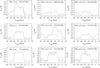 |
Fig. 2 HIFI observations of rotational transitions of ortho-NH3 (left column) and para-NH3 (middle and right columns) are shown by solid lines. Approximated line profiles (see Sect. 2.2) of two blended lines 30(s)−20(a) and 31(s)–21(a) are shown by dot-dashed lines. Emission profiles are overplotted with theoretical profiles (red dashed lines) from our best fit models computed separately for each ammonia spin isomer. The effect of line overlapping in case of the two blends is shown with blue dashed lines. The theoretical profiles for the three lines that were observed at phase φ= 0.13 (see Table 1) are rescaled up to mimic computations at phase φ= 0.23 (see Sect. 4.5 for details). Our approach in searching for the best fit is described in Sect. 4.5, and the best fitting parameters are compiled in Table 2. |
The para-NH3 transition 31(s)−21(a) at 1763.601 GHz (middle panel) overlaps the ortho-NH3 transition 30(s)−20(a) at 1763.524 GHz (upper left panel). Therefore, the shape of the former line was approximated in its blueshifted part using, as a template, a properly rescaled profile of the para-NH3 32(s)−22(a) emission line (middle right panel), which was observed with the same beam size and has a similar excitation. The line profile of the ortho-NH3 transition 30(s)−20(a) was then obtained by subtracting the derived para-NH3 31(s)−21(a) line emission. The resulting profiles are shown by dot-dashed lines in Fig. 2.
2.3. Other observations
To verify our best fit models, we used radio and mid-infrared data for ammonia available from the literature. In this paper, we exploited radio data from Gong et al. (2015), who recently observed five metastable inversion transitions (J,K) = (1, 1), (2, 2), (3, 3), (4, 4), (6, 6) of ortho- and para- ammonia in a 1.3 cm line survey toward IRC+10216. The dates of those observations correspond to phases, φ, from about ~0.62 to ~0.97 (Gong et al. 2015). The half power beam width amounts to 40′′ at the frequency of the inversion lines (about 24 GHz) for observations with the Effelsberg 100 m radio telescope (Gong et al. 2015). Flux densities, Sν in Jy, were converted to main beam temperature Tmb, in K, using the conversion factors suggested by the authors: Tmb/Sν = 1.33 K/Jy for the (6, 6) line at 25 GHz and Tmb/Sν = 1.5 K/Jy for the remaining lines.
By way of comparison with the mid-infrared absorptions of ammonia, we used profiles of the ν2 transitions published by Keady & Ridgway (1993) that were observed at a spectral resolution of 0.009 cm-1 (corresponding to 2.9 km s-1) with the Fourier Transform Spectrometer at the Coudé focus of the 3.8 m Kitt Peak Mayall telescope. Observations of absorption from the metastable rotational levels within the ground vibrational level of ortho- and para-ammonia, aR(0,0), aQ(2,2), aQ(3,3), aQ(4,4), aQ(6,6) were also used for comparison with the results of our modelling. Formally, from the aperture of the telescope, we can estimate the HPBW to be  , using the expression 1.22 × λ/D, where λ is wavelength and D is diameter of the telescope aperture. However, taking into account all instrumental effects, we estimate that the HPBW, in this case, could be as large as 1′′.
3. Ammonia model
Different relative orientations of the spins of the three hydrogen nuclei give rise to two distinct species of NH3: ortho and para. The general criterion governing which levels belong to ortho- and which to para-ammonia is formulated in terms of representations of the molecular symmetry group (see Bunker & Jensen 1998). According to this formalism, ortho states belong to the  and
and  representations of the inversional symmetry group D3h, and para states to the E′ and E′′ representations. For the electronic ground state of ammonia, this translates into the rule that ortho-NH3 has levels with K = 3n, where n = 0,1, ..., and para-NH3 has all other levels. The two species do not interact either radiatively or collisionally. The ortho- to para-NH3 ratio is determined at the moment of the formation of the molecule. Hence, we consider ortho- and para-ammonia as separate molecular species. Transitions of the two species whose frequencies overlap, such as the ortho-NH3 30(s)−20(a) transition and the para-NH3 31(s)−21(a) transition, open the possibility of an interaction through the emission and absorption of line photons. This is considered further in the discussion below.
Ammonia may oscillate in six vibrational modes: the symmetric stretch ν1, symmetric bend ν2, doubly-degenerate asymmetric stretch  , and the doubly-degenerate asymmetric bend
  . Transitions from the ground vibrational state to each of these excited states are observed as vibrational bands at 3, 10, 2.9, and 6 μm, respectively. The band intensities are characterized by the vibrational transition moments 0.027, 0.24, 0.018, and 0.083, respectively (Yurchenko et al. 2011). As long as we consider only the lowest excited vibrational modes, the rule governing the assignment of levels of given K to the ortho and para species, discussed above for the ground state, is preserved for the rotational levels of the symmetric modes and exchanged for the asymmetric ones.
The vibrational ground state of ammonia is split into two states of opposite parities, a consequence of the low energy barrier to inversion of the molecule. Symmetry considerations exclude half of the rotational levels for the K = 0 ladder. Only transitions with ΔK = 0 are electric dipole-allowed. As a result, there is a characteristic doubling of rotational transitions allowed between levels of opposite parities for transitions with K ≠ 0. Forbidden transitions (ΔK ≠ 0) are significantly weaker. Transitions between split sub-levels are allowed as well and give rise to a large number of lines around 23−25 GHz, the so called inversion lines. Their hyperfine structure (hfs) splitting may be neglected in the rotational and vibrational transitions but does influence the line profiles for inversion lines although for IRC+10216, the maximal spread of the hfs components is smaller than the CSE’s expansion velocity. Moreover, the intensities of hfs satellite features relative to that of the main feature (at the central frequency) only become appreciable if an inversion transition (with possible exception of the (1, 1) transition) attains significant optical depth.
The list of transitions and their strengths was extracted from the recent BYTe computations (Yurchenko et al. 2011). In the initial analysis, we extended the sets of molecular data for ortho- and para-NH3 compiled in the LAMDA database (Schöier et al. 2005) by adding energy levels for the excited vibrational states. Two data sets were explored, the first one with only the ν2 = 1 levels, and the second one with ν1 = 1, ν2 = 1 and 2, ν3 = 1, and ν4 = 1 levels. The rotational quantum numbers of the vibrational levels were limited to those originally used in the ground state, i.e. J,K ≤ 7, 7 in ortho- and J,K ≤ 5, 6 in para-ammonia. Both dipole (ΔK = 0) and forbidden (ΔK ≠ 0) transitions between the levels were included.
We found that the inclusion of the ν2 = 1 rovibrational states has a dramatic effect on the flux predicted for the observed pure rotational transitions, when compared with predictions obtained without the inclusion of vibrationally excited states. However, the additional inclusion of the ν1 = 1, ν2 = 2,ν3 = 1, and ν4 = 1 vibrational states has a negligible effect on the computed fluxes for the observed transitions, a maximum increase of only 2 percent being obtained for the flux of the ground rotational transition of ortho-NH3 with even smaller increases for the remaining emission lines. This conclusion, which is based on a model of a molecular structure limited to rotational levels up to J = 7 in each vibrational state, is explained by the fact that the vibrational transition moments to the symmetric bending state are significantly higher than those to the remaining vibrational states. In fact, the radiative pumping rate in the ν2 mode dominates over radiative pumping rates in the remaining modes, even in the innermost parts of the envelope where shorter-wavelength radiation prevails. At larger distances from the star, dust opacity decreases the photon density at shorter wavelengths more effectively, further reducing the relative effect of radiative pumping in other modes. The IR pumping effects for ammonia have been investigated previously by Schöier et al. (2011) and Danilovich et al. (2014).
Solving the radiative transfer, we do not distinguish between photons produced in the envelope and photons coming from the central star. However, by comparing the radiative rates from our best fit model with those obtained when only stellar photons are present, we were able to estimate their relative importance. Only in the inner part of the envelope is radiative excitation in the ν2 transition dominated by the stellar photons. Very quickly, already at seven stellar radii the contribution from the envelope begins to prevail over the contribution from the central star, reaching a ratio of twenty at the outer edge.
Our final model for ammonia includes all levels up to J = 15 in both the vibrational ground state and the ν2 = 1 vibrational state, amounting to a total of 172 levels and 1579 transitions for ortho-NH3 and 340 levels and 4434 transitions for para-NH3. We include the ground state and vibrational levels up to 3300 cm-1, corresponding to 4750 K, above ground. The completeness of the levels used in the computations may be judged by comparing the partition function calculated for the model with that obtained from the full list of lines from the BYTe computations (Yurchenko et al. 2011). With the number of levels given above, the partition function for the ortho species is equal to the BYTe number for temperatures to 300 K, and is lower by 2%, 28%, and 40%, respectively, at 600, 1000, and 1200 K. The partition function of para species is also complete up to 300 K, and is lower by 10%, 40%, and 55%, respectively, at 600, 1000, and 1200 K. The incompleteness in the levels may result in an overestimate of their populations in the dense and hot inner parts of the envelope.
We adopted the collisional rate coefficients from Danby et al. (1988). The rate coefficients for collisional de-excitation are available only for low-lying levels below J = 6 and for a maximum temperature of 300 K. Collisional rates were extrapolated to higher temperatures with a scaling proportional to the square root of the gas temperature. The extension of collisional rates to other levels is necessarily quite crude. At first we neglected collisional rates between levels not available in Danby’s work. In this case, the ladder of levels with K higher than 6 in ortho-ammonia and higher than 5 in para-ammonia are populated only by forbidden radiative transitions. To analyse the influence of the unknown collisional rates on the excitation of NH3, we carried out additional computations based on crude estimates of the collisional rates; here, we adopted collisional depopulation rates of 10-11 or 10-10 cm3 s-1 for rotational states in the ground vibrational state, and rates of 10-14 cm3 s-1 for excited vibrational states. None of these approximations seem to significantly influence our conclusions inferred from the modelling of the observed transitions.
4. Modelling
Here, we present our numerical code and then describe all the assumptions made and parameters investigated during our search for the best fits to the observed rotational transitions of ammonia. After that, we describe the method used to search for the best fit to the data, and present the results thereby obtained.
4.1. Numerical code and procedures
To model circumstellar absorption and emission lines, we developed a numerical code, MOLEXCSE (Molecular Line EXcitation in CircumStelar Envelopes), to solve the non-LTE radiative transfer of molecular lines and the dust continuum. Here, the methodology was to consistently include the effects of optical pumping by the central star and infrared pumping by circumstellar dust upon the population of the molecular levels. The first effect is more critical in the case of post-AGB stars, and the second one more important in AGB stars (see e.g. Truong-Bach et al. 1987). The effect of the dust on the radiation intensity inside the envelope is included by solving the radiative transfer for the line and continuum radiation. For this purpose, the critical properties of the dust – the coefficients of extinction, scattering, and thermal emission – are determined by a separate code by modelling the observed spectral energy distribution of the source, as described in Sect. 4.4. Reproducing the observed continuum fluxes allows the absorption line profiles for mid-infrared vibrational transitions to be computed.
The radiative transfer equation is formulated in the comoving frame (Mihalas et al. 1975) to include the effects of an expanding spherical shell. The only difference is the linearization of the differential equations along tangent rays on a geometrical grid instead of on grid of optical depths. The purpose of this modification was to avoid numerical problems when maser or laser transitions emerge during the iterations.
The simultaneous solution of the statistical equilibrium equations and of the radiative transfer in lines is a non-linear process and, to be efficient, requires linearization of the equations. Full linearization of the radiative transfer equation is very complex and its solution is time-consuming. In the code we follow the approach presented by Schoenberg & Hempe (1986). The original formulation of their approximate Newton-Raphson operator was modified to include the geometrical formulation of radiative transfer mentioned above.
The program possesses two additional features useful in the application to ammonia. First, it enables the simultaneous solution of the radiative transfer problem for more than one molecule. Second, the radiative transfer may be solved with the inclusion of line overlap effects between different molecules. With these features, one can consistently compute the effects of line blending between ortho- and para-NH3. The prominent example of such a case is the overlap between rotational transitions of para-NH3 31(s)−21(a) and of ortho-NH3 30(s)−20(a).
In computing the profiles of the inversion lines, we resolved the hyperfine structure of ammonia, including the effects of quadrupole and magnetic splitting, as measured by Kukolich (1967) and updated by Rydbeck et al. (1977). Line strengths were computed when necessary using the formula given by Thaddeus et al. (1964). These theoretical line strengths are in good agreement with the observed intensities both in laboratory experiments (Kukolich 1967) and in observations of molecular clouds (Rydbeck et al. 1977). The magnetic splitting is much smaller than the quadrupole splitting and has little effect on the line profiles and therefore was neglected in our computations. When solving the radiative transfer, the populations of the sublevels are distributed according to the statistical weights, i.e. assuming local thermodynamical equilibrium (LTE) between sublevels. The relative LTE ratios of intensities as defined by Osorio et al. (2009) were applied including effects of line overlap. The code has been tested by comparison with previously published models of AGB circumstellar envelopes. A detailed description of our code and the tests we conducted will be published elsewhere.
4.2. Thermal and density structure of the envelope
The detailed structure of IRC+10216’s envelope has been the subject of many studies. We mention here only those based on the analysis of CO emission lines (Crosas & Menten 1997; Schöier et al. 2002; Agúndez et al. 2012; De Beck et al. 2012) or the spectral energy distribution (e.g. Men’shchikov et al. 2001).
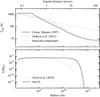 |
Fig. 3 Gas temperature within the envelope of IRC+10216 adopted for this work (upper panel) from Crosas & Menten (1997) is shown by a solid line, while that from De Beck et al. (2012) is shown by a blue dotted line. The dust temperature is shown by a red dashed line. The lower panel shows the distribution of ammonia from our best fitting models (solid line), and its theoretical distribution (dashed line) from Decin et al. (2010). The angular distance is given in the top axis of the upper panel for an assumed distance to IRC+10216 of 130 pc. |
Several models for the thermal structure have been proposed to explain the CO emissions from IRC+10216. These models differ in the assumed distance, mass loss rate and variation of gas velocity in the inner parts of the envelope. For the purpose of this paper, we have chosen, for the basic temperature structure of the envelope, the model of Crosas & Menten (1997), but with the distance reduced from 150 to 130 pc following Groenewegen et al. (2012) (see also Menten et al. 2012). The gas temperature structure of Crosas & Menten (1997) is based on self-consistent computations of the temperature structure and radiative transfer in CO, constrained by observations of CO emissions up to J = 6−5. The adopted distance, expansion velocity and mass loss rate are listed in Table 2 and the gas temperature structure, Tgas, is presented in the upper panel of Fig. 3 by the solid line. The temperature profile has been extended to the inner part of the envelope by assuming a constant value of 1200 K. More recently, De Beck et al. (2012) used the GASTRoNOoM model (Decin et al. 2006, 2010) to derive the gas temperature structure shown by the dashed line in the upper panel of Fig. 3, and found it capable of explaining HIFI observations of CO up to J = 16−15. Figure 3 shows these representative Tgas models to have distinct temperature structures, which differ mainly in the middle part of the envelope.
The density structure of the envelope is computed from the equation of mass conservation, assuming that the gas is entirely composed of molecular hydrogen and that the mass loss rate and outflow velocity are constant. The microturbulent velocity was set to be constant throughout the envelope and equal to 1.0 km s-1 (Crosas & Menten 1997). In fact this value seems to explain the observed shape of the lowest ortho-NH3 10(s)−00(a) emission well.
4.3. Distribution of ammonia
The distribution of ammonia in the circumstellar envelope is governed by the poorly-understood process of ammonia formation, and the well-understood process of its photodissociation in the outer part of the envelope. A detailed chemical model predicting the formation of ammonia and water as a result of photo-processes in IRC+10216 was proposed by Agúndez et al. (2010) (see also Decin et al. 2010). This model predicts peak abundances of ammonia within the observed values but, as we show below, in its present version cannot explain the observed intensities of the rotational transitions.
For the purpose of this paper, we assumed that in the middle parts of the envelope the maximum abundance of ammonia relative to H2, f0, is constant, while in the inner and outer layers it is increasing and decreasing, respectively. To distinguish between ortho- and para-ammonia, their individual abundances are further designated f(ortho-NH3) and f(para-NH3). The abundance profile adopted for the ammonia in the inner layers is based on the model of Decin et al. (2010) (see their supplementary material). For each kind of ammonia, we parametrized the increase of its abundance in the inner parts of the envelope by two free parameters: the formation radius, Rf, and f0. To describe the increase in the ammonia abundance in the inner envelope, we used a fit to the predictions of Decin et al. (2010) of the form f(r) = f0 × 10− 0.434(Rf/r)3, where r is radial distance from the central star. This parametrization, despite its theoretical origin, is a more realistic description of the ammonia distribution than a rather unphysical sharp increase of the ammonia abundance at a fixed radius. We note that Rf may be formally lower than the inner dust shell radius. To describe the decrease in the ammonia abundance near the photodissociation radius, Rph, in the outer layers of the envelope, we used the analytical parametrization f(r) = f0 × exp(−ln2(r/Rph)α), which is frequently used in a parametrization of CO photodissociation (see e.g. Schöier & Olofsson 2001). A slope α = 3.2 was adopted here, in accord with the fit to a detailed chemical model of NH3 photodissociation computed using the CSENV code by Mamon et al. (1988). The ortho- and para-ammonia abundances, the inner radius of ammonia formation, Rf, and its photodissociation radius, Rph, are free parameters in the fitting procedure. The distribution of ammonia from our best-fit models and from Decin et al. (2010) are shown in Fig. 3 by the solid and dashed lines, respectively.
4.4. Dust shell model of IRC+10216
As explained in Sect. 3, the excitation of ammonia is dominated by radiative pumping via the 10 μm ν2 = 1 band. Therefore, to model the ammonia lines we need to estimate the continuum flux at 10 μm inside the whole envelope. For that purpose, we used a dust radiative transfer model (Szczerba et al. 1997), which is able to provide all necessary physical variables to MOLEXCSE. We fit a combination of flux measurements from the Guide Star Catalogue ver. 2.3 (GSC 2.3) for λ<1 μm, photometric data between 1.25 and 5 μm from Le Bertre (1992), and at longer wavelengths from IRAS and COBE DIRBE. In addition, as the strongest constraint, we have used ISO Short Wavelength Spectrograph (SWS) and Long Wavelength Spectrograph (LWS) spectra. They were obtained on May 31 1996 (JD = 2 450 235) and correspond to phase φ of 0.24, counted from the reference maximum phase of the light curve, φ = 0, on November 17 1988 (JD = 2 447 483), and given a period of 649 days (Men’shchikov et al. 2001). We have used this older parameterization of the IRC+10216 variability as it was obtained closer to the date of the ISO observations. For this phase of pulsation and the distance of 130 pc determined recently by Groenewegen et al. (2012), the average luminosity of IRC+10216 was estimated to be about 8500 L⊙ (Men’shchikov et al. 2001; Menten et al. 2012).
As dust constituents, we adopted amorphous carbon of AC type from Rouleau & Martin (1991) and SiC from Pegourie (1988), both with a power-law distribution of grain radii with an index of −3.5 between 0.1 and 0.43 μm. We assumed a maximum allowed dust temperature of 1300 K. We assumed a constant outflow velocity equal to the observed terminal velocity of 14.5 km s-1, in spite of a clear variation of the outflowing velocity in the inner part of envelope seen in higher molecular transitions (Agúndez et al. 2012), and a constant dust mass loss rate. The derived dust mass loss rates were 1.0 × 10⁻⁷M⊙ yr-1 and 3.0 × 10⁻⁹M⊙ yr-1 for AC and SiC dust, respectively. The inner shell radius corresponding to the assumed maximum dust temperature is reached at a distance of about 3 stellar radii. The required total optical depth of the envelope at V is 18.5 mag, which corresponds to τ10 μm equal to 0.18. The parameters of our model for ammonia in IRC+10216 are listed in Table 2 and the mean dust temperature is shown by red dashed line in Fig. 3. As is shown below, the dust temperature determines the radiation intensity in the continuum, which is important for vibrational pumping.
Model for IRC+10216.
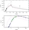 |
Fig. 4 Fit to the flux for Lavg = 8500 L⊙ and effective temperature of 2300 K is shown in both panels by black solid line. The contribution from the central star is shown in the bottom panel by the dash-dotted magenta line. SWS and LWS ISO spectra are shown by red dotted lines. Photometric data below 1 μm are from GSC 2.3, those between 1.25 and 5 μm are from Le Bertre (1992) at three different phases: 0.02 (stars), 0.21 (filled squares) and 0.23 (dotted squares), while at longer wavelengths the flux is from IRAS (crosses) and COBE DIRBE (x) measurements. The dust model obtained for Lmax = 11 850 L⊙ is shown by dashed lines on each panel (see text for details). |
The fit obtained for a stellar luminosity Lavg = 8500 L⊙ and an effective temperature of 2300 K is shown in both panels of Fig. 4 by the black solid line. In our modelling, we did not include MgS, which is commonly used for modelling of the 30 μm structure, since this material has no optical constants in the optical range so the precise determination of its temperature is impossible (see e.g. Szczerba et al. 1997). However, since we are interested in the continuum emission at 10 μm, this approach seems to be justified.
Most of the ammonia lines were observed at phase φ = 0.23 (see Table 1), when the luminosity of the central star was close to its average value Lavg = 8500 L⊙. However, three of the lines were observed at φ ~ 0.13 so, for the purpose of ammonia line modelling, we rescaled their observed integrated area down to φ = 0.13 using the predicted variability from models obtained at maximum and at average luminosity. Since we do not have ISO spectra taken at φ = 0, we cannot constrain the dust properties at the maximum stellar luminosity. Therefore, we decided to recompute our dust model by keeping all parameters (including the inner radius of dust shell) constant, except for the stellar luminosity, which was raised to Lmax. The model results thereby obtained are shown by dashed lines in both panels of Fig. 4.
After modelling the dusty envelope, we exported the dust thermal emission coefficient, along with the total extinction and scattering coefficients, to the code MOLEXCSE, as a function of wavelength and radial distance. MOLEXCSE, which was described above in Sect. 4.1, was then used to solve the multilevel radiative transfer in lines and continuum. See Eq. (1) in Szczerba et al. (1997) for details concerning the exported physical quantities.
4.5. The best-fit models
Using our code described in Sect. 4.1, the ammonia abundance profile given in Sect. 4.3, the model parameters specified in Table 2, together with the gas temperature distribution from Crosas & Menten (1997) and, taking into account vibrational pumping by infrared radiation, we computed a grid of separate models for ortho-NH3 and para-NH3. The grid of models was computed for formation radii Rf = 2.5,5,10,20,40, and 80 R⋆, photodissociation radii Rph ranging from 1.5 × 1016 cm to 6 × 1016 cm in steps of ΔRph = 0.5 × 1016 cm, and f(ortho-NH3) and f(para-NH3) ranging from 1.4 × 10⁻⁸ to 4.8 × 10⁻⁸ in steps of Δf(NH3) = 0.2 ×10⁻⁸.
For each model we defined the figure-of-merit as  (1)where
  (see Table 1) and
  are the observed and theoretically predicted integrated fluxes for the ith line, respectively, σi (see Table 1) is the estimated uncertainty in , and Nlines is 3 for ortho- and 6 for para-NH3 (see Fig. 2). Here, the three lines observed in 2011 at phase φ = 0.13 were rescaled to phase φ = 0.23, assuming that they vary co-sinusoidally between the maximum and average luminosity of the central star. From the computed integrated line fluxes for these stellar luminosities, we obtained the amplitude of their variations as 4.0, 3.1, and 8.2 K km s-1 for the transitions at 1763.524, 1763.601, and 1763.823 GHz, respectively. Since the value of the cosine function describing φ decreases by about 0.6 between phase 0.13 and 0.23, we reduced the integrated fluxes given in Table 1 by 0.6 times the estimated amplitude of the line variations, i.e. by 2.4, 1.9, and 5.0 K km s-1. The quality of each fit is measured by the reduced χ2 parameter, which for two free parameters is defined here as
 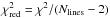 .
.
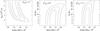 |
Fig. 5 Contours of χ2, indicating the sensitivity of the fit to the model’s free parameters. The left panel shows the dependence of χ2 on the photodissociation radius Rph and abundance of ortho-NH3, given the best fitting value for the formation radius, Rf = 2.5 R⋆. The middle and the right panels show the dependence of χ2 on the formation radius Rf and the abundances of para- and ortho-NH3, given a photodissociation radius Rph = 3 × 1016 cm. The contours correspond to 1, 2, and 3σ confidence levels. The best fits are marked with a cross and the corresponding |
We found that for Rph ≥ 3 × 1016 cm, the minimum value of  is achieved for Rf = 2.5 R⋆ = 1.0 × 1014 cm, which is the minimum formation radius possible for the assumed inner radius of the envelope considered during modelling. However, since the assumed Rph is decreased, the formation radius that minimizes increases (from Rf = 10 R⋆ for Rph = 2.5 × 1016 cm to Rf = 40 R⋆ for Rph = 1.5 × 1016 cm); at the same time, however, the minimum also increases. Hence, the value of the photodissociation radius was found by searching for the minimum among the models for Rf = 2.5 R⋆.
The best fit to the ortho-NH3 lines is achieved for Rph> 2−3 × 1016 cm, and f(ortho-NH3) = (2.8 ± 0.5) × 10-8 at a 3σ confidence level. There is no strong constraint on the maximum value that Rph could have. To estimate the errors, we constructed a χ2 map for ortho-NH3, which is presented in the left panel of Fig. 5, and shows how χ2 varies as a function of the photodissociation radius Rph and f(ortho-NH3) for the best-fit formation radius Rf = 1.0 × 1014 cm. The contours correspond to 1, 2, and 3σ confidence limits. The best fit is indicated with the cross and the corresponding value of  is shown on the plot. Rotational transitions of para-NH3 are even less sensitive to the photodissociation radius, and a plot similar to that shown on left panel of Fig. 5 does not yield any constraints on Rph. This behaviour could be related to the fact that at a given distance from the star the pumping mid-IR radiation is the same, while at low gas temperatures the excitation of the 10(s)−00(a) transition of ortho-ammonia is much more efficient than the excitation of the 21(s)−11(a) transition of para-ammonia (see Fig. 1). On the other hand, the lowest para-NH3 transition, 21(s)−11(a), was observed with HPBW of 18.2′′, corresponding to a projected radius of 1.8 × 1016 cm at the assumed distance of 130 pc; thus, for values of Rph that are larger than this projected radius, this line is less sensitive to Rph than the 10(s)−00(a) ortho-NH3 transition, for which the HPBW is twice as large.
The derived abundance of para-NH3 for the best-fit model is ( , which means that, to within the error bars, the ratio of ortho- to para-NH3 is equal to 1, a ratio that is characteristic of the formation of NH3 at high temperatures (Umemoto et al. 1999). The average abundance for the two species is (3.0 ± 0.6) ×10-8. The error estimate for the para-NH3 abundance given above is the 3σ confidence interval obtained from the χ2 map for para-NH3, which is presented in the middle panel of Fig. 5 and shows how χ2 varies as a function of the formation radius Rf and abundance of para-NH3 at the best-fitting photodissociation radius Rph = 3 × 1016 cm. The meaning of the contours is the same as in the left panel. The best fit, indicated with the cross, and the corresponding are also shown on the plot. The minimum of 0.5 implies an excellent fit to the six para-NH3 lines (with four degrees of freedom).
While the χ2 analysis described above made use of integrated line fluxes instead of the detailed line profiles, the model successfully reproduces the line shapes. The emission line profiles resulting from the best-fit models are shown in Fig. 2 by dashed lines, and the best-fit parameters are listed in Table 2. As indicated in Table 2, the abundances derived for ortho- and para-NH3 are inversely proportional to the assumed mass-loss rate; this can be understood as a consequence of the facts that the NH3 lines are optically thin and that the derived ammonia abundance is only weakly dependent on the exact choice of the gas temperature (see below), so the same total mass of ammonia is required to explain the observations regardless of the mass-loss rate.
To check how strongly the derived best-fit parameters depend on the assumed gas temperature inside the envelope, we performed some test computations using the Tgas structure from De Beck et al. (2012). For the best fitting parameters found above and the Tgas structure of De Beck et al. (2012), we found that the line shapes are only slightly different, but increases to 3.8 for ortho- and to 4.6 for para-NH3. Searching for the model minimizing , we found that the best fit is obtained for a formation radius Rf = 1 × 1014 cm, a photodissociation radius Rph = 3 × 1016 cm, and abundances of ortho-NH3 and para-NH3 equal to ( and (
and ( , respectively. These values lie within the error bounds estimated using the Crosas & Menten (1997) temperature profile, implying that the abundances and photodissociation radius derived from rotational transitions are only weakly dependent on the choice of temperature profile.
Although we obtained the best-fit results based solely on rotational transitions, our model also offers predictions for the other observed transitions. Therefore to make a quality test of our best-fit models, we examined whether they can reproduce both the inversion and mid-IR transitions of ammonia.
While Gong et al. (2015) have obtained observations of the inversion transitions at several different phases (in range 0.20−0.96), our models do not predict any dependence on the integrated fluxes in the phase (i.e. luminosity) of the central star. Calculations show that the expected variation of flux in the (1, 1) inversion line is up to 3 percent between phases of maximum (φ = 0) and mean (φ = 0.25), and is even lower in higher inversion transitions. Thus, our model computed for the average luminosity of the star can be used for comparison with the inversion line observations. Figure 6 shows the observed transitions by means of solid lines (Gong et al. 2015) and the computed theoretical profiles with dashed lines. Vertical sticks mark positions of hyperfine components – the height of the central stick is chosen arbitrary, while the heights of the other sticks are scaled according to their relative theoretical intensities. Our best-fit model for the rotational transitions fits the upper inversion transitions very well, but overestimates the flux measured for the para-NH3 (2, 2) line, and significantly overestimates that for the lowest para-NH3 (1, 1) line. We have found that decreasing Rph to 1.5 ×1016 cm gives a very good fit to the all observed inversion lines (shown by dotted lines in Fig. 6). However, this model is not able to match the rotational lines as successfully as our best-fit model. Using the best-fit abundance of ortho-NH3 and decreasing the photodissociation radius to 1.5 ×1016 cm significantly increases the , to a value 28. On the other hand, the best-fit model with fixed Rph = 1.5 ×1016 cm and free formation radius and abundance of ortho-NH3 moves Rf to about 40 R⋆ and f(ortho-NH3) to 4.2 × 10⁻⁸ with equal to 3.8.
To investigate this discrepancy, we extended the search for the best-fit model by adding the inversion lines. To this purpose, we took the integrated flux from Gong et al. (2015) and converted it to K km s-1 scale. However, our theoretical fit to the inversion lines seems to suggest the presence of hyperfine components, as we describe below in Sect. 5.4 of discussion, at least in the case of the two lowest inversion lines, (1, 1) and (2, 2). Therefore, we repeated the calculation of the integrated flux of these two lines, extending the integration range accordingly. This increased the integrated flux of those two transitions up to about 20% in case the of (1, 1). The integrated fluxes used for the analysis of the inversion lines for ortho-NH3 (3, 3) and (6, 6) transitions are 0.47 ±0.5 and 0.15 ± 0.03 K km s-1, respectively, while for the para-NH3 (1, 1), (2, 2), and (4, 4) transitions are 0.84 ± 0.8, 0.64 ± 0.9, and 0.20 ± 0.4 K km s-1, respectively. Now, considering simultaneously the inversion and rotational lines of para-NH3 put a strong constraint on the photodissociation radius. For the formation radius fixed to the Rf = 1.0 × 1014 cm, we found that the photodissociation radius is Rph = (1.5 ± 0.2) × 1016 cm and the abundance of para-NH3f(para-NH3) = (3.2 ± 0.5)× 10-8 with equal to 0.86. However, the same approach for ortho-NH3 gives rather a different estimation of the photodissociation radius, which is equal to  cm and the abundance of ortho-NH3 equal to (2.4 ± 0.4)× 10-8 with equal to 1.9. Thus, we see, that a global fit gives ortho- and para-NH3 abundances that are quite similar (within error bars) to those obtained from the analysis limited to the rotational lines only. However, the problem of requiring different photodissociation radii for ortho- and para-NH3 remains.
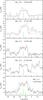 |
Fig. 6 Profiles of the inversion lines as computed for the best-fit models, which assume Rph = 3 × 1016 cm and the Tgas distribution from Crosas & Menten (1997), (blue dotted lines) are overplotted on the observed inversion transitions (solid lines) from Gong et al. (2015). Theoretical profiles for the same Tgas profile, but with the photodissociation radius reduced to Rph = 1.5 × 1016 cm are shown with red dashed lines. Vertical sticks show positions and relative intensities of hyperfine components. |
The infrared transitions to the ν2 levels are seen in absorption against the background dust continuum emission. The observed depths of lines depend on the telecope beam size. In addition, the line spectrum is smoothed by the instrumental profile. The observed ν2 line profiles published by Keady & Ridgway (1993) and synthesized using our best-fit models are shown in Fig. 7. There is reasonable consistency between our model results (dashed line) with the observed profiles (solid line). Some disagreement with the aQ(6, 6) line is most probably due to the neglect of the inner velocity structure of the envelope or to a higher value of the formation radius.
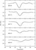 |
Fig. 7 Profiles of NH3 lines in the ν2 band observed by Keady & Ridgway (1993) (solid lines) and synthesized profiles using data from the best-fit models (dashed lines). Theoretical lines have been convolved with a Gaussian profile to achieve a spectral resolution of 2.9 km s-1. |
5. Discussion
5.1. Abundance of ammonia
Over the past 30 yr, the determination of the NH3 abundance in the envelope of IRC+10216 has been the subject of observational studies at radio, mid-infrared, and submillimeter wavelengths. All these observations appeared to provide divergent abundances but, as we discuss below, the main reason for the different results comes from the inclusion (or not) of radiative pumping to the vibrational levels and differences in column densities.
Prior to this study, the only observation of a NH3 rotational transition was made with the spectrograph on board the Odin satellite (Hasegawa et al. 2006). The rather poor signal-to-noise ratio obtained for the lowest 10(s)−00(a) transition of ortho-NH3 did not provide a precise measurement of the line profile. The ammonia abundance relative to H2 was determined as being 1 × 10⁻⁶, significantly above our determination, f(ortho-NH3) = 2.8 × 10⁻⁸. However, the analysis of the line was based on a simplified model of a single K = 0 ladder, limited to the ground vibrational state and, more importantly, neglecting radiative pumping by the infrared radiation. For the adopted model of the IRC+10216 envelope, results from our code show that, with the neglect of IR pumping the abundance of ammonia has to be increased by factor of about 20 to explain the measured 10(s)−00(a) line flux. In addition, the line profile becomes parabolic, which is characteristic of unresolved optically thick emission, in disagreement with the profiles observed by Herschel. Thus, we can conclude that the largest discrepancy in the determination of the ammonia abundance seems to be resolved. The effect of infrared pumping on the molecular abundances derived for evolved stars was previously noted in the paper of Agúndez & Cernicharo (2006), who show that by including the ν2 mode of H2O the abundance of water was decreased by a factor of ≥ 10 with respect to that derived assuming pure rotational excitation. For the specific case of NH3, Schöier et al. (2011) have shown that taking into account IR pumping via vibrationally excited states will decrease the abundance of ammonia by an order of magnitude. In addition, Danilovich et al. (2014) have derived the abundance of ammonia in the S-type star W Aql, including the ν2 state in their analysis of the radiative transfer.
The early observations of the (1, 1) and (2, 2) inversion transitions of para-NH3 around 23 GHz were made by Kwok et al. (1981), Bell et al. (1982), and Nguyen-Q-Rieu et al. (1984). For their assumed distance of 200 pc and mass loss rate of 2 × 10⁻⁵M⊙ yr-1, they found f(para-NH3) as being between 3 ×10⁻⁸ and 2 × 10⁻⁸. At the distance of 130 pc adopted here, and for optically thin transitions, the corresponding values of f(para-NH3) are 0.8 × 10⁻⁸ and 0.5 × 10⁻⁸, respectively, for the assumed mass loss rate of 3.25 × 10⁻⁵. The estimates are a factor of 4 to 6 lower than our determination of para-NH3 abundance, namely  . This difference may be due to simplifying assumptions made in the derivation of the ammonia abundance in these earlier papers. Recently, Gong et al. (2015) have inferred the abundances of ortho- and para-NH3 from observations of their metastable inversion transitions (J,K) = (1,1),(2,2),(3,3),(4,4),(6,6). They lie between 7.1 × 10⁻⁸ to 1.4 × 10⁻⁷ for ortho-NH3, and between 1.1 × 10⁻⁷ and 1.3 × 10⁻⁷ for para-NH3. Here, the assumed mass-loss rate was 2×10⁻⁵M⊙ so, for our adopted mass loss rate, the abundances correspond to values from 4.4 × 10⁻⁸ to 8.6 × 10⁻⁸ for ortho-NH3 and from 6.8×10⁻⁸ to 8.0×10⁻⁸ for para-NH3. Moreover, these values are dependent on the column density of molecular hydrogen, which is uncertain by a factor of 2 (Gong et al. 2015).
Observations of mid-IR ν2 transitions in absorption performed by Betz et al. (1979), Keady & Ridgway (1993) have yielded another estimate of the total abundance of ammonia. For an assumed mass-loss rate of 2 × 10⁻⁵M⊙ yr-1, these two studies inferred total ammonia abundances of 1 × 10⁻⁷ and 1.7 × 10⁻⁷, respectively. Rescaled to our adopted mass-loss rate, these values transform to 6 × 10⁻⁸ and 1 × 10⁻⁷, in agreement with the total ammonia abundance derived by us f(NH3) = (6.0 ± 0.6) × 10-8.
Finally, we note that the remaining differences – at a factor of a few – between the NH3 abundances determined by various methods may not be so significant. The determination of the NH3 abundances using mid-IR absorption ν2 transitions requires an assumption for the column density of ammonia. The values range from about 2 × 1015 cm-2 (Betz et al. 1979; Keady & Ridgway 1993) to 8×1015 cm-2 (Monnier et al. 2000). This may be compared to the total column density along the sight line to the central star in our best-fit model, 1.5 × 1016 cm-2. The different observations average the column density over different parts of the envelope and therefore probe different regions of the CSE. We note that the column density is very sensitive to the densest inner parts of the envelope. For example, for our model with constant velocity and with Rf = 10 R⋆ the total column density drops to only 5 × 1015 cm-2. The assumed velocity profile in the acceleration zone also plays a role. For example, Monnier et al. (2000) had to assume a much higher column density of 8 × 1015 cm-2, by modifying only the behaviour of the velocity field in the inner part of the envelope, while using the model of the dusty envelope similar to the original one from Keady & Ridgway (1993).
5.2. Ammonia formation radius
The best-fit models for ortho- and para-NH3, marked by + signs on the middle and on the right panels of Fig. 5, respectively, are obtained for Rf = 1.0 × 1014 cm or 2.5 R⋆. This means that a lower limit on the ammonia formation radius is not provided by our model fits. On the other hand, the distribution of contours for 1, 2, and 3σ levels on these panels show that ammonia cannot be formed too far from the stellar photosphere. At the 1σ level, the upper limit on the formation radius must be at most 20 R⋆, while at the 2σ level it is around 35 R⋆. This seems to be in rough agreement with the formation radius of ammonia as estimated by Keady & Ridgway (1993) and Monnier et al. (2000) on the basis of their analysis of mid IR lines. The analysis of Keady & Ridgway (1993) allows a distance closer than 10 R⋆, whereas Monnier et al. (2000) conclude that ammonia is formed at a distance ≥ 20 R⋆. This last conclusion was based on interferometric observations of the mid-IR bands in the continuum and at line centre and further modelling of the ratio of visibility functions.
The rotational line profiles of NH3 were fit assuming that the velocity field is constant. However, we performed test computations with the gas velocity field inside the envelope used by Crosas & Menten (1997). We found that they produce a narrow emission feature in the centre of the highest rotational and inversion transitions that are not seen in the observed line profiles. To remove this feature, created by the acceleration region, it was necessary to constrain the formation radius by shifting Rf above 5−10 R⋆, although the quality of the fit – as measured by – was worse in this case. Nevertheless, it seems that the more realistic gas velocity field suggests that ammonia is not formed at the stellar photosphere as suggested by our formal fit to the rotational transitions, assuming a constant outflow velocity.
5.3. Photodissociation radius
The photodisociation radius has been constrained by observations of the of the NH3 (1, 1) and (2, 2) inversion lines (Nguyen-Q-Rieu et al. 1984). Their analysis of the observed lines required a cut-off of the molecular abundance beyond a radius of (0.6−1)×1017 cm at the assumed distance of 200 pc. This corresponds to (4.0−6.5) × 1016 cm at distance assumed in this paper, d = 130 pc, and is in the range allowed by our modelling, Rph> 2−3 × 1016 cm. Models for the NH3 distribution in the circumstellar envelope of IRC+10216 presented by Decin et al. (2010), and shown by the dotted line in Fig. 3, predict a decrease in the ammonia abundance in the outer envelope that is more rapid than is allowed by the observations. With this type of distribution, we cannot fit the rotational lines of ammonia, especially the lowest transition of ortho-NH3, since its upper level is underpopulated at still quite high gas temperatures (see Figs. 1 and 3). Similarly, this is also the case for the reduced photodissociation radius inferred from the fit to the observations of inversion lines by Gong et al. (2015).
5.4. Line shapes
Thanks to the high signal-to-noise ratio (S/N) obtained for the ortho-NH310(s)−00(a) spectrum, the details of the line profile are well-constrained (see bottom left panel in Fig. 2). Another line, the 32(s)–22(a) line at 1763.823 GHz, was also observed at a high S/N ratio and has an identical shape (see the middle right panel in Fig. 2). The energy of the upper level for these two transitions is quite different (29 and 127 K, see Table 1), and the similarity of their shapes suggests that both of them are excited in a rather similar region within the envelope. Surprisingly, their shapes show two peaks resembling the profiles of resolved optically thin transitions. However, this is not possible because, given the Herschel beam size at the frequency of the 10(s)−00(a) transition, it would require an outer radius for the ammonia-emitting region to be in excess of 1017 cm, a value close to the CO photodissociation radius. Very similar shapes of rotational lines of SiO (J = 2−1 through J = 7−6 in their ground vibrational state) have been observed in IRC+10216 with the IRAM 30-m telescope by Agúndez et al. (2012) (see their Fig. 4), who suggested that the observed peaks may be formed by additional excitation provided by shells with enhanced density observed in the outer layers of the envelope of IRC+10216 (see e.g. Cernicharo et al. 2015). The line shape can also indicate the presence of spiral shells (Decin et al. 2015) in the inner envelope, and/or a hole in the middle of the envelope in the ammonia distribution.
Another possible hypothesis that explains the slightly double-peaked shape of NH3 rotational transitions could be additional excitation of levels by line overlap. In particular, this effect may couple ortho- and para-NH3 levels. This hypothesis has been tested by simultaneous computations of both ortho and para species including effects of line overlap. We found, however, that this process cannot explain the asymmetric double-peak line profiles that are observed. On the other hand, it does reproduce the resulting composite profile of the overlapping transitions (para-NH331(s)–21(a) at 1763.601 GHz and ortho-NH3 30(s)−20(a) at 1763.524 GHz) shown in Fig. 2 by the long dash line.
The theoretical profiles for the inversion transitions show a complex structure, due to the overlap of emission in the hyperfine components. In particular, the profile of the para-NH3 (1, 1) line (see the lowest panel in the Fig. 6) shows at least the central and the two long wavelength components of the hyperfine multiplet. The two narrow peaks at −32 and −20 km s-1 caused by the overlap of the blue edge of one component and red edge of the next one further confirms the presence of at least one of the short wavelength components. Observations with higher S/N would probably reveal the shortest wavelength component.
6. Summary
We present Herschel/HIFI observations obtained with high spectral resolution for all nine rotational transitions up to the J = 3 levels for ortho- and para-NH3 in the envelope of the C-rich AGB star IRC+10216. Using our numerical code MOLEXCSE, which solves the non-LTE radiative transfer in molecular lines and dust continuum, we searched for the best-fit parameters that explain all three ortho- and six para-NH3 rotational lines. Computations were done separately for ortho- and para-NH3. Three free parameters were constrained by the modelling effort: the ammonia formation radius, its photodissociation radius and the abundance. The best fits were obtained when infrared pumping of NH3 was included, using the gas temperature structure from Crosas & Menten (1997), which is representative of self-consistently computed Tgas structures. Test computations with the gas temperature profile of De Beck et al. (2012) showed that, while the fit obtained is slightly worse, the best-fit parameters are only weakly sensitive to the assumed temperature structure.
We found that the best fit to the rotational lines is obtained if the abundance of ortho- and para-NH3 are equal to (2.8 ± 0.5) ×10-8 and (, respectively. The fit, including both rotational and inversion lines, gives the ortho- and para-NH3 abundances that are quite similar (within the error bars) to those obtained from the analysis limited to the rotational lines only (f(ortho-NH3) = (2.4 ± 0.4)× 10-8 and f(para-NH3) = (3.2 ± 0.5)× 10-8). These values are compatible with an ortho/para ratio of one, characteristic for the formation of ammonia at high temperatures. The derived abundance of ortho-NH3 has solved the long-lasting problem of the discrepancy between the abundance derived from the lowest submillimeter rotational line and those from radio inversion or infrared absorption transitions. It was found that the main process that brought the abundances of ammonia derived from different spectral transitions close to each other was the inclusion of the NIR radiative pumping of ammonia via the 10 μm ν2 = 1 band. The average abundance of NH3 derived from rotational lines agree to within of a factor a few with those from radio inversion or infrared absorption transitions, and we argued that this difference may not be significant, since both methods rely on an uncertain determination of the ammonia column density.
In addition, since the MOLEXCSE code also offers predictions for other NH3 transitions in the radio and mid-IR range, we tested whether our best-fit models were able to explain the observations of Gong et al. (2015) and Keady & Ridgway (1993). In the case of the inversion transitions, we found that reducing Rph to 1.5 × 1016 cm gives a very good fit to the lower para-NH3 (1, 1) and (2, 2) inversion transitions, but with so small a Rph that the fit to the rotational lines of ortho-NH3 is significantly worse. We admit, however, that our best fit model for the rotational transitions may overpredict the envelope size as a result of inaccuracies in modelling of the inner parts of the envelope. In the case of the MIR absorption lines, we found that our best-fit model reproduces the observed profiles from Keady & Ridgway (1993) fairly well. Some disagreement with the aQ(6,6) line profile is most probably due to our neglect of the inner velocity structure in the envelope.
The ammonia formation radius is not well-constrained in our approach, and the best fitting abundances of ortho- and para-NH3 were obtained at the minimum value of the formation radius considered in our analysis, 2.5 R⋆. The best fits were obtained assuming that the outflow velocity is constant, so we performed test computations with the gas velocity, increasing inside the acceleration zone. We found that for Rf = 2.5 R⋆ this type of velocity field produces a narrow emission feature in the centre of the highest inversion transitions that is not seen in the observed line profiles. To remove this feature, created in the acceleration region, it was necessary to shift Rf above 5−10 R⋆, still inside the 1σ limits obtained from fitting the line strengths. Nevertheless, the more realistic gas velocity field suggests that ammonia is not formed at the stellar photosphere as had been suggested by the formal fits to the rotational transitions, assuming a constant gas velocity field.
A lower limit on the ammonia photodissociation radius seems to be implied by our fit to the rotational transitions, while the maximum value for Rph is unconstrained. Our value of (2−3) × 1016 cm seems to agree quite well with other determinations. However, the best fit to the both rotational and inversional transitions does not give fully consistent results for the ortho- ( cm) and para-NH3 (Rph = (1.5 ± 0.2) × 1016 cm). Furthermore, a distribution of NH3 with the fast decrease predicted by the model of Decin et al. (2010) does not yield a good fit to the lowest rotational transitions of ortho-ammonia.
The two rotational lines that have the highest S/N (10(s)−00(a) of ortho- at 572.498 GHz and 31(s)–21(a) of para-NH3 at 1763.601 GHz) show two asymmetric peaks in their profile. These can be due to an excess of radiation from almost concentric rings or spiral shells as suggested in literature. We also investigated the possibility that they result from the coupling of the ortho- and para-NH3 levels by the effects of line overlap. The computations showed that this process cannot explain the observed peaks, but it can successfully account for the 31(s)–21(a) at 1763.601 GHz and ortho-NH3 30(s)–20(a) line at 1763.524 GHz.
Acknowledgments
M.S.c. and R.S.z. acknowledge support by the National Science Center under grant (N 203 581040). J.H.e. thanks the support of the NSFC research grant No. 11173056. Funded by Chinese Academy Of Sciences President’s International Fellowship Initiative. We acknowledge support from EU FP7-PEOPLE-2010-IRSES programme in the framework of project POSTAGBinGALAXIES (Grant Agreement No. 269193). Grant No. 2015VMA015. V.B., J.A. and P.P. acknowledge support by the Spanish MICINN, program CONSOLIDER INGENIO 2010, grant “ASTROMOL” (CSD2009-00038), and MINECO, grants AYA2012-32032 and FIS2012-32096. J. Cernicharo thanks Spanish MINECO for funding under grants AYA2009-07304, AYA2012-32032, CSD2009-00038, and ERC under ERC-2013-SyG, G.A. 610256 NANOCOSMOS. L.D. acknowledges funding by the European Research Council under the European Community’s H2020 program/ERC grant agreement No. 646758 (AEROSOL). K.J. acknowledges the funding from the Swedish national space board. D.A.N. was supported by a grant issued by NASA/JPL. HIFI has been designed and built by a consortium of institutes and university departments from across Europe, Canada and the United States under the leadership of SRON Netherlands Institute for Space Research, Groningen, The Netherlands and with major contributions from Germany, France and the US. Consortium members are: Canada: CSA, U.Waterloo; France: CESR, LAB, LERMA, IRAM; Germany: KOSMA, MPIfR, MPS; Ireland, NUI Maynooth; Italy: ASI, IFSI-INAF, Osservatorio Astrofisico di Arcetri- INAF; Netherlands: SRON, TUD; Poland: CAMK, CBK; Spain: Observatorio Astronómico Nacional (IGN), Centro de Astrobiología (CSIC-INTA); Sweden: Chalmers University of Technology – MC2, RSS & GARD; Onsala Space Observatory; Swedish National Space Board, Stockholm University – Stockholm Observatory; Switzerland: ETH Zurich, FHNW; USA: Caltech, JPL, NHSC. HCSS/HSpot/HIPE is a joint development by the Herschel Science Ground Segment Consortium, consisting of ESA, the NASA Herschel Science Center, and the HIFI, PACS and SPIRE consortia.
References
- Agúndez, M., & Cernicharo, J. 2006, ApJ, 650, 374 [NASA ADS] [CrossRef] [Google Scholar]
- Agúndez, M., Cernicharo, J., & Guélin, M. 2010, ApJ, 724, L133 [NASA ADS] [CrossRef] [Google Scholar]
- Agúndez, M., Fonfría, J. P., Cernicharo, J., et al. 2012, A&A, 543, A48 [NASA ADS] [CrossRef] [EDP Sciences] [Google Scholar]
- Becklin, E. E., Frogel, J. A., Hyland, A. R., Kristian, J., & Neugebauer, G. 1969, ApJ, 158, L133 [NASA ADS] [CrossRef] [Google Scholar]
- Bell, M. B., Kwok, S., & Feldman, P. A. 1980, in Interstellar Molecules, ed. B. H. Andrew, IAU Symp., 87, 495 [NASA ADS] [Google Scholar]
- Bell, M. B., Kwok, S., Matthews, H. E., & Feldman, P. A. 1982, AJ, 87, 404 [NASA ADS] [CrossRef] [Google Scholar]
- Betz, A. 1987, in Astrochemistry, eds. M. S. Vardya, & S. P. Tarafdar, IAU Symp., 120, 327 [Google Scholar]
- Betz, A. L., McLaren, R. A., & Spears, D. L. 1979, ApJ, 229, L97 [NASA ADS] [CrossRef] [Google Scholar]
- Bunker, P. R., & Jensen, P. 1998, Molecular symmetry and spectroscopy, 2nd edn. (Ottawa, Canada: NRC Research Press) [Google Scholar]
- Cernicharo, J., Marcelino, N., Agúndez, M., & Guélin, M. 2015, A&A, 575, A91 [NASA ADS] [CrossRef] [EDP Sciences] [Google Scholar]
- Cherchneff, I. 2012, A&A, 545, A12 [NASA ADS] [CrossRef] [EDP Sciences] [Google Scholar]
- Cheung, A. C., Rank, D. M., Townes, C. H., Thornton, D. D., & Welch, W. J. 1968, Phys. Rev. Lett., 21, 1701 [Google Scholar]
- Crosas, M., & Menten, K. M. 1997, ApJ, 483, 913 [NASA ADS] [CrossRef] [Google Scholar]
- Danby, G., Flower, D. R., Valiron, P., Schilke, P., & Walmsley, C. M. 1988, MNRAS, 235, 229 [NASA ADS] [CrossRef] [Google Scholar]
- Danilovich, T., Bergman, P., Justtanont, K., et al. 2014, A&A, 569, A76 [NASA ADS] [CrossRef] [EDP Sciences] [Google Scholar]
- De Beck, E., Lombaert, R., Agúndez, M., et al. 2012, A&A, 539, A108 [NASA ADS] [CrossRef] [EDP Sciences] [Google Scholar]
- de Graauw, T., Helmich, F. P., Phillips, T. G., et al. 2010, A&A, 518, L6 [NASA ADS] [CrossRef] [EDP Sciences] [Google Scholar]
- Decin, L., Hony, S., de Koter, A., et al. 2006, A&A, 456, 549 [NASA ADS] [CrossRef] [EDP Sciences] [Google Scholar]
- Decin, L., Agúndez, M., Barlow, M. J., et al. 2010, Nature, 467, 64 [NASA ADS] [CrossRef] [PubMed] [Google Scholar]
- Decin, L., Richards, A. M. S., Neufeld, D., et al. 2015, A&A, 574, A5 [NASA ADS] [CrossRef] [EDP Sciences] [Google Scholar]
- Gong, Y., Henkel, C., Spezzano, S., et al. 2015, A&A, 574, A56 [NASA ADS] [CrossRef] [EDP Sciences] [Google Scholar]
- Groenewegen, M. A. T., van der Veen, W. E. C. J., & Matthews, H. E. 1998, A&A, 338, 491 [NASA ADS] [Google Scholar]
- Groenewegen, M. A. T., Barlow, M. J., Blommaert, J. A. D. L., et al. 2012, A&A, 543, L8 [NASA ADS] [CrossRef] [EDP Sciences] [Google Scholar]
- Harju, J., Walmsley, C. M., & Wouterloot, J. G. A. 1993, A&AS, 98, 51 [NASA ADS] [Google Scholar]
- Hasegawa, T. I., Kwok, S., Koning, N., et al. 2006, ApJ, 637, 791 [NASA ADS] [CrossRef] [Google Scholar]
- Herbig, G. H., & Zappala, R. R. 1970, ApJ, 162, L15 [NASA ADS] [CrossRef] [Google Scholar]
- Ho, P. T. P., & Townes, C. H. 1983, ARA&A, 21, 239 [NASA ADS] [CrossRef] [Google Scholar]
- Jijina, J., Myers, P. C., & Adams, F. C. 1999, ApJS, 125, 161 [NASA ADS] [CrossRef] [Google Scholar]
- Keady, J. J., & Ridgway, S. T. 1993, ApJ, 406, 199 [NASA ADS] [CrossRef] [Google Scholar]
- Kirsanova, M. S., Wiebe, D. S., Sobolev, A. M., Henkel, C., & Tsivilev, A. P. 2014, MNRAS, 437, 1593 [NASA ADS] [CrossRef] [Google Scholar]
- Kukolich, S. G. 1967, Phys. Rev., 156, 83 [NASA ADS] [CrossRef] [Google Scholar]
- Kwok, S., Bell, M. B., & Feldman, P. A. 1981, ApJ, 247, 125 [NASA ADS] [CrossRef] [Google Scholar]
- Le Bertre, T. 1992, A&AS, 94, 377 [NASA ADS] [Google Scholar]
- Mamon, G. A., Glassgold, A. E., & Huggins, P. J. 1988, ApJ, 328, 797 [NASA ADS] [CrossRef] [Google Scholar]
- McLaren, R. A., & Betz, A. L. 1980, ApJ, 240, L159 [NASA ADS] [CrossRef] [Google Scholar]
- Men’shchikov, A. B., Balega, Y., Blöcker, T., Osterbart, R., & Weigelt, G. 2001, A&A, 368, 497 [NASA ADS] [CrossRef] [EDP Sciences] [Google Scholar]
- Menten, K. M., Wyrowski, F., Alcolea, J., et al. 2010, A&A, 521, L7 [NASA ADS] [CrossRef] [EDP Sciences] [Google Scholar]
- Menten, K. M., Reid, M. J., Kamiński, T., & Claussen, M. J. 2012, A&A, 543, A73 [NASA ADS] [CrossRef] [EDP Sciences] [Google Scholar]
- Mihalas, D., Kunasz, P. B., & Hummer, D. G. 1975, ApJ, 202, 465 [NASA ADS] [CrossRef] [Google Scholar]
- Miller, J. S. 1970, ApJ, 161, L95 [NASA ADS] [CrossRef] [Google Scholar]
- Monnier, J. D., Danchi, W. C., Hale, D. S., Tuthill, P. G., & Townes, C. H. 2000, ApJ, 543, 868 [NASA ADS] [CrossRef] [Google Scholar]
- Mueller, M., Jellema, W., Olberg, M., Moreno, R., & Teyssier, D. 2014, The HIFI Beam: Release 1, Release Note for Astronomers, Tech. Rep. HIFI-ICC-RP-2014-001, v1.1, HIFI-ICC [Google Scholar]
- Neufeld, D. A., González-Alfonso, E., Melnick, G., et al. 2010, A&A, 521, L5 [NASA ADS] [CrossRef] [EDP Sciences] [Google Scholar]
- Neufeld, D. A., Tolls, V., Agúndez, M., et al. 2013, ApJ, 767, L3 [NASA ADS] [CrossRef] [Google Scholar]
- Nguyen-Q-Rieu, Graham, D., & Bujarrabal, V. 1984, A&A, 138, L5 [NASA ADS] [Google Scholar]
- Nguyen-Q-Rieu, Winnberg, A., & Bujarrabal, V. 1986, A&A, 165, 204 [NASA ADS] [Google Scholar]
- Osorio, M., Anglada, G., Lizano, S., & D’Alessio, P. 2009, ApJ, 694, 29 [NASA ADS] [CrossRef] [Google Scholar]
- Pegourie, B. 1988, A&A, 194, 335 [NASA ADS] [Google Scholar]
- Pilbratt, G. L., Riedinger, J. R., Passvogel, T., et al. 2010, A&A, 518, L1 [CrossRef] [EDP Sciences] [Google Scholar]
- Roelfsema, P. R., Helmich, F. P., Teyssier, D., et al. 2012, A&A, 537, A17 [NASA ADS] [CrossRef] [EDP Sciences] [Google Scholar]
- Rouleau, F., & Martin, P. G. 1991, ApJ, 377, 526 [NASA ADS] [CrossRef] [Google Scholar]
- Rydbeck, O. E. H., Sume, A., Hjalmarson, A., et al. 1977, ApJ, 215, 35 [Google Scholar]
- Schoenberg, K., & Hempe, K. 1986, A&A, 163, 151 [NASA ADS] [Google Scholar]
- Schöier, F. L., & Olofsson, H. 2001, A&A, 368, 969 [NASA ADS] [CrossRef] [EDP Sciences] [Google Scholar]
- Schöier, F. L., Ryde, N., & Olofsson, H. 2002, A&A, 391, 577 [NASA ADS] [CrossRef] [EDP Sciences] [Google Scholar]
- Schöier, F. L., van der Tak, F. F. S., van Dishoeck, E. F., & Black, J. H. 2005, A&A, 432, 369 [NASA ADS] [CrossRef] [EDP Sciences] [Google Scholar]
- Schöier, F. L., Maercker, M., Justtanont, K., et al. 2011, A&A, 530, A83 [NASA ADS] [CrossRef] [EDP Sciences] [Google Scholar]
- Szczerba, R., Omont, A., Volk, K., Cox, P., & Kwok, S. 1997, A&A, 317, 859 [NASA ADS] [Google Scholar]
- Thaddeus, P., Krisher, L. C., & Loubser, J. H. N. 1964, J. Chem. Phys., 40, 257 [NASA ADS] [CrossRef] [Google Scholar]
- Truong-Bach, Nguyen-Q-Rieu, Omont, A., Olofsson, H., & Johansson, L. E. B. 1987, A&A, 176, 285 [NASA ADS] [Google Scholar]
- Truong-Bach, Morris, D., & Nguyen-Q-Rieu. 1991, A&A, 249, 435 [NASA ADS] [Google Scholar]
- Umemoto, T., Mikami, H., Yamamoto, S., & Hirano, N. 1999, ApJ, 525, L105 [NASA ADS] [CrossRef] [PubMed] [Google Scholar]
- Walmsley, C. M., & Ungerechts, H. 1983, A&A, 122, 164 [NASA ADS] [Google Scholar]
- Wienen, M., Wyrowski, F., Schuller, F., et al. 2012, A&A, 544, A146 [NASA ADS] [CrossRef] [EDP Sciences] [Google Scholar]
- Yurchenko, S. N., Barber, R. J., & Tennyson, J. 2011, MNRAS, 413, 1828 [NASA ADS] [CrossRef] [Google Scholar]
All Tables
All Figures
|
Fig. 1 Diagram of energy levels of ortho- (|K| = 0, 3, etc.) and para-NH3 (|K| = 1, 2, 4, etc.). The inversion splitting between levels of different symmetry is exaggerated for clarity. The observed rotational transitions with frequencies in GHz are indicated with arrows. |
| In the text | |
|
Fig. 2 HIFI observations of rotational transitions of ortho-NH3 (left column) and para-NH3 (middle and right columns) are shown by solid lines. Approximated line profiles (see Sect. 2.2) of two blended lines 30(s)−20(a) and 31(s)–21(a) are shown by dot-dashed lines. Emission profiles are overplotted with theoretical profiles (red dashed lines) from our best fit models computed separately for each ammonia spin isomer. The effect of line overlapping in case of the two blends is shown with blue dashed lines. The theoretical profiles for the three lines that were observed at phase φ= 0.13 (see Table 1) are rescaled up to mimic computations at phase φ= 0.23 (see Sect. 4.5 for details). Our approach in searching for the best fit is described in Sect. 4.5, and the best fitting parameters are compiled in Table 2. |
| In the text | |
|
Fig. 3 Gas temperature within the envelope of IRC+10216 adopted for this work (upper panel) from Crosas & Menten (1997) is shown by a solid line, while that from De Beck et al. (2012) is shown by a blue dotted line. The dust temperature is shown by a red dashed line. The lower panel shows the distribution of ammonia from our best fitting models (solid line), and its theoretical distribution (dashed line) from Decin et al. (2010). The angular distance is given in the top axis of the upper panel for an assumed distance to IRC+10216 of 130 pc. |
| In the text | |
|
Fig. 4 Fit to the flux for Lavg = 8500 L⊙ and effective temperature of 2300 K is shown in both panels by black solid line. The contribution from the central star is shown in the bottom panel by the dash-dotted magenta line. SWS and LWS ISO spectra are shown by red dotted lines. Photometric data below 1 μm are from GSC 2.3, those between 1.25 and 5 μm are from Le Bertre (1992) at three different phases: 0.02 (stars), 0.21 (filled squares) and 0.23 (dotted squares), while at longer wavelengths the flux is from IRAS (crosses) and COBE DIRBE (x) measurements. The dust model obtained for Lmax = 11 850 L⊙ is shown by dashed lines on each panel (see text for details). |
| In the text | |
|
Fig. 5 Contours of χ2, indicating the sensitivity of the fit to the model’s free parameters. The left panel shows the dependence of χ2 on the photodissociation radius Rph and abundance of ortho-NH3, given the best fitting value for the formation radius, Rf = 2.5 R⋆. The middle and the right panels show the dependence of χ2 on the formation radius Rf and the abundances of para- and ortho-NH3, given a photodissociation radius Rph = 3 × 1016 cm. The contours correspond to 1, 2, and 3σ confidence levels. The best fits are marked with a cross and the corresponding |
| In the text | |
|
Fig. 6 Profiles of the inversion lines as computed for the best-fit models, which assume Rph = 3 × 1016 cm and the Tgas distribution from Crosas & Menten (1997), (blue dotted lines) are overplotted on the observed inversion transitions (solid lines) from Gong et al. (2015). Theoretical profiles for the same Tgas profile, but with the photodissociation radius reduced to Rph = 1.5 × 1016 cm are shown with red dashed lines. Vertical sticks show positions and relative intensities of hyperfine components. |
| In the text | |
|
Fig. 7 Profiles of NH3 lines in the ν2 band observed by Keady & Ridgway (1993) (solid lines) and synthesized profiles using data from the best-fit models (dashed lines). Theoretical lines have been convolved with a Gaussian profile to achieve a spectral resolution of 2.9 km s-1. |
| In the text | |
Current usage metrics show cumulative count of Article Views (full-text article views including HTML views, PDF and ePub downloads, according to the available data) and Abstracts Views on Vision4Press platform.
Data correspond to usage on the plateform after 2015. The current usage metrics is available 48-96 hours after online publication and is updated daily on week days.
Initial download of the metrics may take a while.