| Issue |
A&A
Volume 591, July 2016
|
|
|---|---|---|
| Article Number | A128 | |
| Number of page(s) | 16 | |
| Section | Extragalactic astronomy | |
| DOI | https://doi.org/10.1051/0004-6361/201527149 | |
| Published online | 28 June 2016 | |
Mid-infrared interferometry of Seyfert galaxies: Challenging the Standard Model
Leiden Observatory, Leiden University, PO Box 9513, 2300 RA Leiden, The Netherlands
e-mail: This email address is being protected from spambots. You need JavaScript enabled to view it.
Received: 9 August 2015
Accepted: 19 October 2015
Abstract
Aims. We aim to find torus models that explain the observed high-resolution mid-infrared (MIR) measurements of active galactic nuclei (AGN). Our goal is to determine the general properties of the circumnuclear dusty environments.
Methods. We used the MIR interferometric data of a sample of AGNs provided by the instrument MIDI/VLTI and followed a statistical approach to compare the observed distribution of the interferometric measurements with the distributions computed from clumpy torus models. We mainly tested whether the diversity of Seyfert galaxies can be described using the Standard Model idea, where differences are solely due to a line-of-sight (LOS) effect. In addition to the LOS effects, we performed different realizations of the same model to include possible variations that are caused by the stochastic nature of the dusty models.
Results. We find that our entire sample of AGNs, which contains both Seyfert types, cannot be explained merely by an inclination effect and by including random variations of the clouds. Instead, we find that each subset of Seyfert type can be explained by different models, where the filling factor at the inner radius seems to be the largest difference. For the type 1 objects we find that about two thirds of our objects could also be described using a dusty torus similar to the type 2 objects. For the remaining third, it was not possible to find a good description using models with high filling factors, while we found good fits with models with low filling factors.
Conclusions. Within our model assumptions, we did not find one single set of model parameters that could simultaneously explain the MIR data of all 21 AGN with LOS effects and random variations alone. We conclude that at least two distinct cloud configurations are required to model the differences in Seyfert galaxies, with volume-filling factors differing by a factor of about 5–10. A continuous transition between the two types cannot be excluded.
Key words: radiative transfer / galaxies: active / galaxies: Seyfert / techniques: high angular resolution
© ESO, 2016
1. Introduction
Active galactic nuclei (AGN) have been extensively studied to understand the possible link between the growth of supermassive black holes (SMBHs) and the evolution of galaxies. The main characteristic of AGNs is their extremely high luminosity. In particular, AGNs are known to emit a large part of their energy in the form of infrared radiation (Neugebauer et al. 1979; Barvainis 1987; Sanders et al. 1989; Elvis et al. 1994, and references therein). This infrared excess can be explained by a conversion process where a fraction of the nuclear UV and optical radiation is absorbed by circumnuclear dust at a few parsecs from the central black hole and re-emitted in the infrared regime. This circumnuclear dust, commonly referred to as the dusty torus, not only redistributes the emitted energy of AGNs, but sometimes also blocks our view of the nuclear engine.
According to the Standard Model for AGNs, all Seyfert galaxies are assumed to have a similar nuclear environment, consisting of an accreting supermassive black hole surrounded by ionized clouds moving at high velocities (the broad emission line region: BLR). This nuclear engine is then surrounded by circumnuclear dust. In its most simple form, the Standard Model predicts a bimodal distribution of the Seyfert types (Antonucci 1993; Urry & Padovani 1995): type 1, for which the nuclear engine can be directly viewed, and type 2, for which the view to the central engine is blocked by dust. This idea is supported by the broad emission lines in the spectra of many type 2 sources observed in polarized light (see, e.g., Antonucci & Miller 1985).
Studying the properties and morphology of the circumnuclear dust is crucial to improve our understanding of the accretion process of AGNs. It is unclear as yet how the gas flows into the accretion disk, but tracing the coexisting dust can help to reveal the morphology of the gas stream. This process of transport to the inner regions is poorly understood, but is relevant for understanding the triggering and evolution of AGNs as well as the energy feedback to the host galaxy.
High-resolution infrared images of the circumnuclear dust are expected to allow tracing the structure of these objects and determining their general properties. But infrared observations of the AGN environment that isolate and resolve the torus emission have been difficult to obtain. Early observations with the Spitzer telescope provided studies of AGN samples (see, e.g., Buchanan et al. 2006). Their sensitivity allowed statistical studies on a large number of detected objects, but their limited spatial resolution did not accurately isolate the AGN emission from sources of contamination, such as star-heated dust and dust in the ionization cones (Bock et al. 2000; Tomono et al. 2001; Packham et al. 2005). In contrast, large ground-based mid-infrared (MIR) instruments, with their higher resolution power, can distinguish between AGN emission and star formation regions (e.g., Galliano et al. 2005; Alonso-Herrero et al. 2006, 2011; Horst et al. 2006, 2008, 2009; Haas et al. 2007; Siebenmorgen et al. 2008; Levenson et al. 2009; Ramos Almeida et al. 2009, 2011; Hönig et al. 2010; Reunanen et al. 2010; van der Wolk et al. 2010; Mason et al. 2012; Asmus et al. 2011, 2014). However, in the majority of the cases the AGN emission remained unresolved, suggesting either a small size for the nuclear dusty environment or potential nonthermal contributions such as the synchrotron emission observed in the radio galaxy Centaurus A.
Mid-infrared interferometers have enabled a breakthrough by spatially resolving the compact emission of AGNs. Several studies of individual galaxies have revealed the complexity of the nuclear dusty environment. A few examples of these findings are that the nuclear dust environment of the Circinus galaxy shows a two-component structure consisting of a disk-like emission surrounded by an extended emission with its major axis close to the polar axis (Tristram et al. 2014); the hot and compact dusty disk in the nucleus of NGC 1068 shows extended and diffuse emission along one side of its ionization cone (Raban et al. 2009; López-Gonzaga et al. 2014); NGC 424 and NGC 3783 show extended thermal infrared emission with major axes close to the polar axes (Hönig et al. 2012, 2013). In addition, Tristram & Schartmann (2011) analyzed a sample of sources observed with interferometers and suggested a luminosity-size relation for the warm dust. This relation was later challenged by Kishimoto et al. (2011b) using a sample of type 1 sources. It seemed similarly unlikely in the light of results obtained using a larger sample of AGNs, the MIDI AGN Large Programme (Burtscher et al. 2013), which revealed a diversity of complex dust morphologies on subparsec scales. The diversity of sizes suggests that a luminosity-size relation might not be unique for the warm dust as it is in the case of the hot dust observed in the near-infrared (Barvainis 1987; Suganuma et al. 2006; Kishimoto et al. 2009, 2011a; Weigelt et al. 2012), where the inner radius of the torus scales with the square root of the AGN luminosity.
From the theoretical point of view, much progress has been made in recent years in reproducing the infrared emission of the dusty torus with radiative transfer models. Early radiative transfer models of AGN dust tori were carried out by Pier & Krolik (1992, 1993) and Granato & Danese (1994) using smooth dust distributions. However, such a smooth dust distribution probably does not survive in the nuclear environment of an AGN (Krolik & Begelman 1988), but might instead be present in the form of clouds. Pioneer work from Nenkova et al. (2002) presented a stochastic torus model with dust distributed in clumps that is capable of attenuate the strength of the silicate feature. More recently, many torus models, using different radiative transfer codes, techniques, and dust compositions, have been developed to obtain more efficient and accurate solutions of the radiative transfer equations and to improve the assumptions (Nenkova et al. 2002, 2008a,b; Dullemond & van Bemmel 2005; Hönig et al. 2006; Schartmann et al. 2008; Hönig & Kishimoto 2010; Stalevski et al. 2012; Heymann & Siebenmorgen 2012; Siebenmorgen et al. 2015).
However, all the models face one common problem: the dynamical stability of the structure and the process to maintain the required scale height are still debated. Self-consistent models describing both the physical processes that distribute the toroidal gas and dust and the redistribution of the nuclear emission are still under development, but with promising results (see, e.g., Dorodnitsyn et al. 2011, 2015; Wada 2012; Schartmann et al. 2014, and references therein).
Many authors have fit the spectral energy distributions (SEDs) of Seyfert galaxies with clumpy torus models (see, e.g., Nikutta et al. 2009; Mor et al. 2009; Ramos Almeida et al. 2009; Alonso-Herrero et al. 2011; Ichikawa et al. 2015), but the conclusions from these works must be examined critically. Since the SEDs contain no direct spatial information on the torus, the results are highly degenerate; results from a comparison between clumpy and continuous models indicate that models using different assumptions and parameters can produce similar SEDs (Feltre et al. 2012). We may expect the degeneracies to be partially broken if we include high-resolution interferometric observations that resolve the structures and provide direct measures of the sizes and shapes of the emission regions.
The aim of this work is to find a family of torus models that fits the interferometric data on a set of AGNs obtained over the past decade. We focus more on the general properties of the acceptable models than on particular characteristics provided by individual fits. The paper is organized as follows: the main goals and motivation are explained in Sect. 2. We provide information about the Seyfert sample and describe the data treatment in Sect. 3. A brief explanation about the torus models used for this work and the method followed for our comparison is given in Sects. 4 and 5, respectively. The results are presented in Sect. 6. We discuss the general properties in Sect. 7. A summary of the results is given in Sect. 8.
2. Probabilistic approach
Ideally, multiwavelength high-quality infrared images of several AGNs would determine the most important dust model parameters, such as cloud sizes, disk inner radii, wavelength-dependent extensions, opening angles, and dust chemistry. However, high-fidelity infrared imaging is not yet possible since interferometric techniques are time consuming and lack detailed phase data, and their resolution is not high enough to resolve individual clouds. This situation is expected to improve in a few years when the next generation of interferometers come online, for instance, GRAVITY (Eisenhauer et al. 2011), which will observe in K-band, and MATISSE (Lopez et al. 2008), which will observe in L, M, and N-band.
Our ability to determine the underlying parameters of clumpy models is also limited by their stochastic nature; even when all parameters are specified, random variations in the cloud distributions may present markedly different images to the observer.
These limitations necessitate a probabilistic approach to modeling. Our main goal is to investigate whether we can statistically reproduce the data of our whole interferometric sample by using models that have specified global properties, but where the appearance of each source is affected by unknown factors (Vi with i = 1,2,3): 1) the randomness in the positions of the clouds, 2) the inclination, and 3) the position angle of the source axis on the sky. The stochastic arrangement of the clouds can produce different families of spectra or images of the model even when they are built with the same global parameters (Hönig et al. 2006; Schartmann et al. 2008). The torus inclination angle is of primary importance because it determines the chance of viewing directly (low inclinations) or indirectly (high inclinations) heated clouds. The position angle is an important unknown when only limited interferometric baselines are available.
We aim to find global properties that the AGNs might have in common and to test with these the existence of any overall unifying model of AGNs. Our procedure is to search for a model that explains all the observations on a statistical basis. If this fails (as it does), we consider the possibility that the model parameters may vary from object to object, or for certain classes of objects. This is the case if our models can fit each galaxy or class individually, but not all of them for one parameter set.
3. Observational data
Source properties.
3.1. Infrared data
Our sample consists of 21 Seyfert galaxies observed with the MID-infrared Interferometric instrument (MIDI1Leinert et al. 2003) at the European Southern Observatory’s (ESO’s) Very Large Telescope. This flux-limited sample was published by Burtscher et al. (2013), who required sources with a flux higher than 300 mJy at λ ~ 12 μm in high-resolution single-aperture observations. For more specific information about the reduction process and observation strategy we refer to Burtscher et al. (2013). The original set also includes data for the quasar 3C 273 and the radio source Cen A, but we omit these two sources as their nuclear MIR emission may not originate in the same way as in Seyfert galaxies. For example, the nuclear MIR flux of Cen A is dominated by unresolved emission from a synchrotron source, while the contribution of the thermal emission of the dust only represents about 40% of the total emission at 12 μm (Meisenheimer et al. 2007). We exclude the quasar 3C 273 because the MIR environment of high-luminosity objects might differ from that of low-luminosity objects (Seyfert galaxies) sources (see, e.g., Stern 2015).
Each source was observed with pairs of 8 m unit telescopes (UTs), and Circinus and NGC 1068 were additionally observed with pairs of 1.8 m auxiliary telescopes (ATs), in at least three different baseline configurations. The main observable of the instrument MIDI is the correlated flux, which can be seen as the measured fraction of the total flux that is coherent for a particular (u,v) point2.
To capture the shape of each interferometric spectrum and to reduce the computational time, we used three different wavelengths in our fits. We took the average values at (8.5 ± 0.2) μm, (10 ± 0.2) μm and (12 ± 0.2) μm rest frame, whereby we include information about the slope and the amplitude of the silicate feature.
4. Clumpy torus models
Since we cannot create images from our MIR interferometric data, we need to make use of models to interpret our observations. The dusty cloud models used for this work are based on the approach followed before by Schartmann et al. (2008). In this section we briefly explain some of the general aspects of the models, but for more details we refer to Appendix A. These models are built with dense spherical dusty clouds distributed randomly throughout a defined volume. The temperature distributions within these cloud arrangements are quite complex and need to be solved numerically by using radiative transfer codes. The overall dust temperature distribution of the dust and the scaling properties of the torus are essentially determined by the strength of the heating source and the fraction of the UV emission that the dust clouds intercept.
The models used for this work are characterized by the following parameters (Pi): (1) The total average optical depth at 9.7 μm along the equator; (2) the opening angle defining the dust-free cone; (3) the local fractional volume occupied by the dusty clouds at 1 pc given by the filling factor; (4) the radial extension of the dusty torus defining the outer radius; and (5) the density profile index α that defines the radial density profile of the clouds. The modifications to the original model presented by Schartmann et al. (2008) are as follows.
-
Isotropic emission of the central source. We omit the|cos(θ)| law profile emission of the original model as there is no evidence for a strong anisotropy in the MIR−X-ray relation (see, e.g., Ichikawa et al. 2012).
-
We define our filling factor at the inner 1 pc region instead of taking the whole volume space. N-band fluxes are sensitive to dust with a temperature near 300 K, and for the nuclear luminosities LUV used in our modeling, most of the dust at this temperature is found at a radius of ~1 pc.
We used the radiative transfer code RADMC-3D3 to compute the temperature and the surface brightness distributions of the dusty torus. First the temperature of the system was computed by sending out photon packages using a Monte Carlo approach. Anisotropic scattering was treated using the Henyey-Greenstein approximate formula (Henyey & Greenstein 1941). After computing the temperature of the dust grains, we used the included ray tracer to obtain the surface brightness maps at the required wavelengths. We computed high-resolution model images for different lines-of-sight (a given φ and θ angle in the coordinate system of the model) at three different wavelengths, 8.5 μm, 10.0 μm, and 12.0 μm. To determine the corresponding Seyfert type of the images along a line-of-sight (LOS), we took the respective value of the optical depth in the visual τV and classified them as type 1 if τV < 1 and type 2 if τV > 1, that is, type 1 if there is a direct view of the nucleus and type 2 if the nucleus is obscured. Finally, to obtain the correlated fluxes, we applied a discrete fast Fourier transform to each image.
For every parameter set, we computed at least ten different realizations of the model to estimate the variations that are due to the position of the clouds. For every realization we extracted the images along ten different LOS corresponding to type 1 objects and also ten LOS where the nucleus is obscured (type 2 objects).
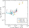 |
Fig. 1 Absorption-corrected 2−10 keV X-ray fluxes versus nuclear 12 μm fluxes. |
4.1. Luminosity rescaling
The luminosity of the central engine obviously is a key parameter in determining the appearance of the source. To match our model images with the observational data for any particular source, we required an accurate estimate of the nuclear UV luminosity to scale the size of the observed objects with the size of the model images. Since it is usually not possible to directly measure the UV emission of the accretion disk, we examine here one of the commonly used tracers for the UV luminosity: the absorption-corrected 2–10 keV X-ray luminosity.
Several studies (see, e.g., Lutz et al. 2004; Horst et al. 2008; Gandhi et al. 2009; Levenson et al. 2009; Ichikawa et al. 2012; Asmus et al. 2015) have reported a tight correlation between absorption-corrected 2−10 keV X-ray and MIR luminosities for Seyfert galaxies, which has been interpreted as a direct connection between the luminosity of the accretion disk and the luminosity of the torus. In Fig. 1 we show the MIR fluxes from Burtscher et al. (2013) and the absorption-corrected 2–10 keV X-ray fluxes from Asmus et al. (2015). We used fluxes instead of luminosities to avoid false correlations induced by the spread in redshifts. The correlation is unclear and the X-ray flux is spread over about one decade for sources with essentially the same MIR flux.
Because the relation of the X-ray and UV as well as the significant scatter in the MIR-Xray is unclear, we decided to avoid using LX as a proxy for LUV. Instead we assumed a nominal nuclear isotropic heating luminosity Lm as part of the modeling process and adjusted its value for each model so that the single-aperture 12 μm predicted by the model matches the observed value. The observed single-aperture fluxes are in general accurately measured. This Lm was used to rescale the model sizes and fluxes, as described below.
The nominal luminosity Lm is the energy emitted from the nucleus that then iluminates the clouds and generates the 12 μm emission. This luminosity is effectively the same as LUV, although it might differ slightly if the dust at the inner radius is not modeled accurately. Although we cannot strictly check the accuracy of this nominal luminosity because we lack near-infrared (NIR) measurements, we expect the deviations to be only mild as the hot emission is treated consistently in our models. Thus any possible deviation from the true LUV might occur if a completely different prescription for the ensemble of clouds were used in the enviremissiononment close to the sublimation radius.
The images described in the previous section were computed for a nominal model nuclear UV luminosity Lm (1.2 × 10¹¹L⊙) at a nominal model distance Dm. These must be compared to the MIR observations of sources at an actual distance Ds computed from the redshift and actual nuclear luminosity Ls, which is assumed to be unknown.
For this comparison, we mathematically moved the model to Ds and then adjusted Lm until the total infrared continuum emission toward the observer at λ = 12 μm equaled the observed 12 μm single-aperture flux. This adjustment was calculated for each model realization, including the cloud distribution and the inclination angle θ, because these factors affect the fraction of the nuclear luminosity converted from UV into infrared and then projected toward the observer, that is, the observed UV-IR efficiency, ηUV−IR.
Adjusting the nuclear luminosity would a priori involve recalculating the radiation transferred through the cloud distribution for each realization. Fortunately, scaling relations in the radiation transfer obviate this computationally expensive step. Assuming that the grain size distribution remains constant, we expect the inner dust sublimation radius rin to scale as  because the temperature of dust grains exposed directly to nuclear UV should only depend on the flux,
  . So we may intuitively expect a source with a given Ls to resemble one with Lm, but all emitted luminosities are scaled by Ls/Lm and all dimensions scaled by (Ls/Lm)1/2. We directly tested this scaling relation with the RADMC-3D models over variations of a factor of 10 in Lm and found it to apply with high accuracy, even for emission from regions not directly heated by the nucleus. In other words, the spatial distribution of the infrared radiation at all wavelengths considered here scales directly with rin.
For a full description of our procedure we refer to Appendix B.
5. Description of the method
5.1. Stochastic modeling
In Sect. 2 we explained that with our data, studies of individual sources may not determine uniquely the parameters Pi underlying the stochastic models. A statistical method dealing with the entire dataset may give better insight into these parameters.
We sought a statistical method that is robust and relatively familiar, so that bad fits can be easily diagnosed. The second criterion suggests a variant of the χ2-test method. Several difficulties immediately arose. First, the interferometric dataset is very inhomogeneous; measurements were made of galaxies of different luminosities, at different distances, position angles, and baselines. Second, some of the measures are highly correlated with respect to the stochastic variables Vi. Finally, the actual selection criteria of the sample are also quite inhomogeneous.
We circumvented the first two problems by using the information provided by the models to find transformations that convert the measurements CFuv,n to new uncorrelated, zero-mean, unit-variance variables cfuv,n. For each model we produced a large number of realizations of the stochastic variables Vi: source orientation, inclination, and cloud positions. For each galaxy the individual measurements CFuv,n, that is, the correlated fluxes at each (u,v) position, were simulated for each of the model realizations after adjusting for the source luminosity described in Sect. 4.1. These simulations produced a probability distribution of simulated measurements  for the galaxy that were then convolved with the distribution of noise estimates from the actual measurements CFuv,n. If the model is correct, the true data values should then lie within the most likely parts of the distributions (65% of the distribution for a Gaussian-like distribution). A very poor model can be rejected at this phase if the individual measurements CFuv,n lie outside the predicted ranges. But models can also be rejected if the total set of data, per galaxy or group of galaxies, is unlikely, and for this we have to consider the expected correlations between the measurements.
The distributions are characterized by their means and (co)-variances. For a given model we now constructed for each galaxy a new set of variables cfuv,n from the original measurements CFuv,n by first subtracting the mean expectation values predicted from the models and then computing linear combinations of the measurements that diagonalize the cross-correlation matrix to unit values. These new variables therefore have zero mean, unit variance, and zero cross-correlation if the model is correct. In this way we can test for any single galaxy, or any set of galaxies, the acceptability of the model by summing the squares of the transformed variables cfuv,n and comparing the total with that expected from the sum of the same number of normal Gaussian variables, that is, a χ2-distribution with the given number of degrees of freedom. We note that models can be rejected if the squared sum is either too large (measurements do not look like the model) or too small (model predicts variances that are larger than the measured values).
5.2. Selection effects
We now considered the inhomogeneous selection criteria. The large program sample was chosen from well-known relatively nearby southern Seyfert galaxies, whose nuclear single-aperture N-band fluxes were above 300 mJy. When we test whether a specific model could account for a single (u,v) measurement or for all the measurements on one galaxy, this selection process is not critical to the interpretation. In this case, we only gauge whether there is some mildly probable cloud configuration that matches that data. When instead we test whether the data from all sample galaxies, or a subgroup of these galaxies, can be explained by a single model, we have to consider the selection effects. The data distributions calculated above were found by assuming that all the stochastic variables are uniformly distributed. The selection process may skew these distributions. For example, if a cloud distribution tends to extinguish N-band emission in the equatorial plane, galaxies with dust structures viewed edge-on will be less likely to meet the 300 mJy limit. This would contradict the assumption of a random distribution of inclination angles.
To account for this, we considered the efficiency ηUV−IR of converting nuclear UV emission into MIR emission directed toward the observer. Each model cloud realization yields a different calculable value for this efficiency. Low-efficiency realizations require a higher and therefore less probable nuclear luminosity for the MIR flux to exceed the survey limit SIR. Therefore we modeled the effect of the MIR flux selection on the model distributions by reweighting each stochastic realization proportional to the probability that the nuclear luminosity Lnuc exceeds  . Hard X-ray surveys of Seyfert nuclei (Georgantopoulos & Akylas 2010) indicate that the integral luminosity function, that is, the probability that the luminosity exceeds a specified value Lnuc, scales approximately as
  with γ ≃ 1. Thus we can model the effect of the flux selection on the observed distributions by reweighting each realization in proportion to
  .
.
Similarly, we introduced a reweighting to model the selection of the galaxies as Seyfert AGNs in the first place. The principle Seyfert classifications depend on the escape of hard UV photons from the hot accretion disk to the narrow line region (NLR), which is well outside our modeling region, where they induce high-excitation ionization. We modeled this effect by calculating for each realization the UV-escape efficiency ηesc for UV photons to escape the cloud regions and by reweighting the realization proportional to  .
.
The effects of these reweighting schemes on the best-fitting model parameters are described in more detail below.
Input parameters.
Best-fit parameters.
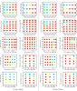 |
Fig. 2 Discrete maps showing the level of acceptance around the best-fit solution for type 1 sources (first and second column) and type 2 sources (second and third column). In every panel, three of the five parameters of the best solution are kept fixed, while the two parameters shown in the labels of each plot are explored. The best-fit solution is shown with an asterisk. The color of the squares indicates the acceptance value of the parameters based on a χ2-test. The blue squares indicate the probability of the χ2-value using the equivalent percentages of a Gaussian distribution at the 1σ level (68%), green the probability at 95% confidence, yellow up to 99.5% and red above 99.5%. |
6. Results
It is very time consuming to computate the temperature profile and the respective images of every realization, therefore we explored the parameter space using a discrete set of values. The values taken for each parameter are shown in the top section of Table 3, together with other input parameters. To account for a bias that is due to the detection limit of the sample, our results were obtained using a reweight, as stated in Sect. 5.2, with a value of γ = 1.
6.1. Full sample
We first analyzed our entire sample containing Seyfert 1s and 2s together. We searched for the best combination of parameters Pi that statistically describe our sample. In all our mapping space we did not find any set of parameters Pi that produces models consistent with our entire sample of AGNs. Within our range of parameters, this result suggests that our sample is not consistent with the idea that their observed differences should only be attributed to a LOS effect; this is consistent with the result of Burtscher et al. (2013).
Our entire sample cannot be reproduced statistically by a single set of model parameters Pi, while each individual galaxy can be fit by its own set of parameters Pi,n. This suggests two possible cases. First, AGNs cannot be explained with one fixed set of parameters Pi, but instead we need a broad range of parameters Pi. Alternatively, there are major subgroups within the sample, each of which can be fit with its own set of parameters Pi. When searching for the best set of parameters, we observed that occasionally the type 2 objects and some of the type 1 objects were consistent with each other, but a significant fraction of type 1s seemed to be poorly fit. This motivated us to investigate both types independently to search for their best-fit models. A reasonable set of parameters that describes our subsets would allow us to explain why we failed to fit the two groups together.
6.2. Type 1
We continued our search in the parameter space using the type 1 set, that is, sources where our view to the nucleus is not blocked by the dust. In the models, this means taking LOS that penetrate the dust-free volume inside of the opening angle and LOS at high inclinations that by chance do not encounter clouds along its path. For this set of objects we did find combinations of model parameters that produced a distribution of correlated fluxes that is compatible in a probabilistic sense with the observational data. The range of model parameters that shows a best fit with the data are listed in Table 3. Additionally, we plot in Fig. 2a discrete maps showing the behavior of the level of acceptance when we let two parameters change freely around the best solution. We display these confidence levels as color-coded plots for different pairs of input parameters. This allows the viewer to decide quickly whether the best-fitting parameters are correlated, or in other words, whether particular combinations of parameters are better constrained than the individual parameters themselves.
We observe from Fig. 2a that for the type 1 subset the best-constrained parameters are the volume-filling factor, the radial density profile index, and the optical depth. Only model spatial filling factors at 1 pc radius between 0.4% and 1.4% fit the type 1 observations at better than the 3σ level. As we explain in more detail in the discussion section, the low percentages for the filling factor are necessary to produce a diverse family of spectra and sources with multiple sizes without using different parameters Pi for every object. Because the clouds are somewhat larger than in other available models (Hönig et al. 2006; Nenkova et al. 2008a), realizations in our models with low filling factors and steep radial density profiles have a very limited number of total individual clouds, between 5−10 clouds on average.
We also obtain a good estimate for the total radial optical depth at 9.7 μm. This parameter must be on the order of or higher than τ9.7 μm = 8, corresponding to a value in the optical of τ0.5 μm ≳ 75. Lower values for the optical depth all yield fits equivalent to 4σ or worse for a normal distribution. A combination of high optical depths and inclination effects allows a reduction of the silicate feature. In this case the shadowing effect explained by Schartmann et al. (2008) might not be too strong because there are only a few clouds.
With the low filling factor of the type 1s, we anticipate that the index of the radial density profile for the clouds may be poorly constrained. The low number of clouds may not allow an accurate determination of the density profile. Still, we observe in Fig. 2a that only steep radial distributions, with an index lower than −1, agree with our observations, meaning that clouds are more likely to be found at close or intermediate distances (a few tenths of the sublimation radius). Sets of models with a low filling factor at the inner radius but flatter distributions instead produce an excess of cold emission because a many clouds could exist at large distances, while the number of clouds at the smallest distances can be kept low.
The maximum radial extension is poorly constrained in our models because we lack long-wavelength infrared data. In all the plots that show the radial extension the fits are good for all the possible values. Because the best-fit parameters have a steep radial cloud distribution, not many clouds exist at large radius. If present, clouds at large distances will be dominated by cold emission (<100 K) and should be detected at (sub-) millimeter wavelengths. The opening angle for a limited number of clouds does not make much sense as the distribution of clouds along the azimuthal direction produces similar results for different opening angles. We observe in the two lower plots of Fig. 2a that the opening angle is essentially good in the range used for our search, 30−60 deg. This behavior is expected when the number of clouds is low.
6.3. Type 2
After finding the best-fit parameters for the type 1 objects, we searched for the best-fit parameters for the type 2 objects to see if the deviate from the type 1 sample. Since our models are wedge-like structures, the type 2 LOS are confined within a region outside the opening angle.
We found several sets of parameters Pi that reproduce the type 2 observations. The range of best-fit parameters found for this subset are shown in Table 3, and variations of the level of acceptance when changing two parameters around the best-fit solution can be seen in Fig. 2b.
For type 2 Seyfert galaxies, the radial slope of cloud distribution is steep, similar to the type 1 sources. The acceptable index for the density profile lies between −2 and −1. Again, because of this steep slope and the lack of long-wavelength infrared data, the maximum radial extension of the torus is poorly defined.
The main difference between Figs. 2a and b is the range of acceptable values for the filling factor. For the type 2 sources, the number of clouds at the inner regions is significantly larger for than the type 1 sources. The acceptable filling factors for the type 2 sources are larger than ~5%. This means that the cloud-filled volume near 1 pc is a factor of 5 or higher than that in the type 1s. This suggests an important intrinsic difference between types 1 and 2.
The average optical depth throughout the whole disk at 9.7 μm is similar for the type 2 models to that of the type 1 models. Any optical depth value above 8 gives reasonable fits. Increasing the value of τ beyond ~8 makes no difference; by this time, all the N-band photons have been absorbed and converted to even longer wavelengths.
A higher filling factor at the inner radius for type 2s and similar density profile index with respect to type 1s means that type 2 objects have a larger total number of clouds. With similar values of the optical depth for both types, but type 2s having a higher total number of clouds means that for type 2s it is more likely to observe dusty clouds along the LOS. The fewer clouds in the type 1 model result in a lower covering fraction and larger (u,v) variations for an individual type 1 with respect to a typical type 2.
The best value for the opening angle lies near 60°. Models with opening angles of 45° are in the 2σ or 3σ region, those with opening angles of 30° are quite unlikely since they are in the 4σ area. For small opening angles the images along obscured LOS of these models will look more or less round, while models with large opening angles essentially produce flat disks. A study of the elongations in the Large Program sources suggests an intrinsic ratio of 1:2 (López-Gonzaga et al. 2016). Therefore, a roundish model might not be a good representation of the dusty structure of sources such as NGC 1068 and Circinus, especially because these two objects both have a disk-like component and a near-polar extended component. These two moderate-luminosity galaxies are so close that the long baseline interferometric measurements represent a physical resolution that is not obtainable for any of the other survey galaxies. To include them in our analysis on a comparable basis to the others, we only included interferometric measurements for these two at projected baselines <40 m, which only includes information about the extended component and an unresolved component (the disk resolved with higher projected baselines). Therefore, it is likely that due to the arbitrary location of the axis system in our analysis, the best-fit model is influenced by the elongations of the sources, and as a result, fixing the opening angle produces the required elongations (1:2) but with an incorrect system axis.
6.4. Line-of-sight selection
Since the same input bolometric was used for all the models, using a weight means that bright images are more likely to be observed, since the ratio between the infrared and UV is lower than faint images in the infrared. For high optical depths this causs the images with high self-absorption to be rarer. We applied the same weighting exponent to both type 1 and 2 throughout all our work. Only type 2 sources show a clear difference when using the reweight. The 12 μm emission of the type 1 sources is less likely to be affected by self-absorption of the dust. The dispersion of the 12 μm fluxes for a particular model for type 1 objects is not very broad, and therefore the reweighting does not play an important role.
For type 2 objects this reweighting is quite relevant. For high-inclination values, the 12 μm fluxes can be more affected by the self-absorption of the dust clouds. In Fig. 3 we show a comparison for different parameters using a rescaling with γ = 1 and without weights. The greatest difference is that if we do not use the reweighting, models with low filling factors become likely for type 2 sources. The reason for this is that in these types of models the hot surfaces of the individual clouds produce similar bright spots in the large scales as the surfaces produced by models with high filling factors, where the emission in the large-scale structure is produced by escaping emission through holes. The rescaling we performed to match the fluxes and distances of the real sources modifies the sizes and aligns them with those given by our interferometric measurements. Although the geometry generally looks similar, the problem of not using a reweighting is that for type 2 models with low filling factors the ratio between the bolometric luminosity and the infrared luminosity becomes extremely high, some of ratios are even quite unrealistic, as seen from the luminosity function of Seyfert galaxies.
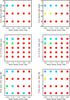 |
Fig. 3 Comparison of the discrete maps for models of type 2s using (left) no luminosity reweighting and (right) a more realistic reweighting with γ = 1. |
7. Discussion
7.1. What does the interferometer see?
In this section we examine the images of the best models to acquire intuitive insight into their structures, and to understand which features in the models cause noticeable differences in the actual observations.
Our work shows that apparent differences in the MIR morphology arise not only from inclination effects, but that statistical variations in the cloud distribution can be relevant as well. When the size of the clouds is large enough and the fraction of the volume occupied by the clouds is relatively low, the appearance of the MIR emission will vary depending on our specific LOS and realization of the models (Hönig et al. 2006; Schartmann et al. 2008). In the probabilistic models presented by Nenkova et al. (2008a,b), these variations do not appear explicitly because their models are built using average quantities, therefore differences that are due to statistical variations of the clouds are ignored.
In Fig. 4 (top) we plot the observed interferometric 12 μm visibilities of our objects using measurements along two distinct position angles if available. The baselines are rescaled to compensate for their luminosities and distances, as described in Sect. 4.1. To the right of the same figure we plot the model visibilities for different realizations of type A and type B models that would have been classified as a Seyfert 1 galaxy because the nucleus is directly visible. In Fig. 5 we show model images of four realizations of type A models and in Fig. 6 images of type B models with unobscured nuclei. The lower plots in Fig. 4 and the images in Fig. 7 represent observations and models of Seyfert 2 galaxies and type B models with obscured nuclei. Except for two objects in the left top plot of Fig. 4, when normalized in the infrared, low-luminosity objects seem to be better resolved than high-luminosity objects.
The plot of Fig. 4 (top left) shows large variation in visibilities of the Seyfert 1 galaxies, which is reproduced by the low filling factor type A models. The type B unobscured models show much less variation and relatively high visibilities because more clouds in the model are located closer to the inner regions of the torus, making is seem compact and smooth. Figure 5 shows that the appearance of the low filling factor models is determined by the positions of a few hot, bright, unobscured clouds around the nucleus. The random variations of the positions of these clouds in the realizations creates the large variations in apparent visibility. This creates the apparently uniform high visibilities in these models. It is clear from the plots that the curves from the high filling factor type B model cannot reproduce the overall distribution of observed visibilities for our full sample of type 1 objects: the variation in visibilities would be too low. Objects such as NGC 3783, IC 4239A, and NGC 4593 have large dispersions in their visibilities that cannot be explained with the type B model. Although the aim of this work is not to find the physical explanations for the dusty structure, we note that the three mentioned objects have lower luminositis than the less resolved objects (e.g., IRAS 13349+2438). We cannot, of course, exclude that some of the type 1 galaxies represent unobscured type B geometries, a situation similar to the original Standard Model.
For Seyfert 2 galaxies, images from obscured LOS of type B models are shown in Fig. 7. With the nuclear regions blocked by dust, the emission is dominated by the accidental positions of relatively free LOS through holes in the cool dust to warmer areas at various radii. These accidents produce the variations in visibility seen in the bottom plots of Fig. 4. Once again, a few of the observed Seyfert 2 galaxies may arise from type A low-density geometries where the LOS is blocked by a stray cloud.
7.2. Spectral energy distribution.
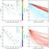 |
Fig. 4 Left: 12 μm interferometric visibilities of type 1 (top) and type 2 sources (bottom) plotted against the normalized projected baseline. For every object we include visibilities for two different position angles connected by independent lines. The normalized baseline is scaled from the observed baseline for each source to normalize its single-aperture 12 μm flux; cf. Sect. 4.1. Each symbol indicates the longest baseline data point available at the given position angle for an individual object. The color of the symbols indicates the value of the infrared luminosity of the source as shown on the scale at the right, data are from by Table 1. Top right: model normalized 12 μm interferometric radial plots for various lines of sight where the nucleus is exposed, corresponding to type 1 objects, computed from type A models (blue) and from type B models (red). Bottom right: model radial plots for various obscured LOS, corresponding to type 2 objects, computed for the best type B models. |
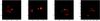 |
Fig. 5 12 μm images created from one of the best type 1 models (model A). We only show lines-of-sight where the nucleus is exposed. Each plot shows a different realization of the cloud positions. Labels denote the distance to the center in pc. |
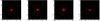 |
Fig. 6 Same as Fig. 5, but the images are created from the unobscured lines-of-sight from model B, i.e., type 1s with the same filling factor as type 2 objects. |
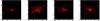 |
Fig. 7 Same as Fig. 5, but the images are created from the obscured lines-of-sight from model B, i.e., the best type 2 model. |
We only analyzed the N-band data, where the new interferometric measurements include more spatial information than the single-aperture spectral energy distributions (SEDs) alone. Ideally, we should describe the SED and interferometric data simultaneously. We did not attempt this because of the difficulties of consistently calibrating multiwavelength observations, the very different resolutions and fields of view of these observations, possible contamination from other physical sources, and lack of multiwavelength observations for most of our objects.
In spite of these problems, we can produce the SEDs with the radiative transfer code over broad wavelength ranges for our best-fit models with the purpose of displaying the overall predicted behavior of the spectra. The SEDs presented in this work can be further investigated by us or other groups to verify them outside the MIR window. In particular in the near-infrared, the promising technique presented by Burtscher et al. (2015) for isolating the NIR emission of the AGN is expected to provide good constraints for the hot emission.
We show examples of different realizations of the best type 1 model for unobscured inclinations (in Fig. 8a) and for obscured inclinations using the best type 2 model (Fig. 8c). We also include the SEDs of unobscured inclinations for the best type 2 model in Fig. 8b. The SEDs corresponding to different realizations of obscured type 2 objects show a diverse family of spectra with variations of the silicate feature in absorption. Similar to other torus models, the modeled spectra only show a moderate absorption feature in contrast to the deep silicate feature typically present in continuous models. From Fig. 8c we observe that it is also possible to obtain SEDs with relatively high emission at short wavelengths from hot dust coupled with small silicate absorption features. It is quite likely that such SEDs correspond to regions with holes in the cloud distribution through which the hot emission from the inner regions is seen, giving rise to a significant contribution of flux in the near-infrared. The small silicate feature in this case could be explained as an average between the absorption feature produced from the back faces of the clouds and the silicate feature in emission that is viewed through the holes of the torus. This could explain the absence of a silicate feature in absorption and the relatively blue spectra of NGC 424 described by Hönig et al. (2012).
The main differences between the SEDs of the true type 1 models and those of the unobscured type 2 models are in the strength of the silicate feature and the slope of the spectrum in the 2−20 μm wavelength range. The silicate features in true type 1 models vary from weak absorption to moderate emission; the spectral slopes vary from moderately hot (large near-IR contribution) to moderately cool; the warmth of the continuum slope is directly correlated with the strength of the emission feature. For the unobscured type 2 models the silicate feature is always seen weakly in emission and the continuum spectrum (in units of λLλ) weakly rising toward shorter wavelengths.
In Fig. 9b we zoom into the 8−12 μm single-aperture spectra for the observed objects, as well as the output spectra from their respective best-fit models. The multiple spectra are generated from different realizations and multiple inclinations of the best-fit model. In the top row we observe that the spectra of type 1 objects agree well with the predictions of the model. The diversity of slopes and the featureless spectra seem to be well described. As a comparison, we additionally include the interferometric spectra from the lowest baseline available. Many of our type 1 objects are slightly resolved with the shortest baseline resolution, so the differences in the shape of the spectra are small. If contamination by surrounding starburst regions is present in the single-aperture spectra, however, the shortest baseline spectrum should be less affected by this. The observed type 2 spectra are also well reproduced by the best-fit modeled spectra. Objects with deep silicate features can be explained with our model, although they are less common.
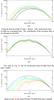 |
Fig. 8 SEDs for multiple realizations of the best-fit model. |
7.3. Are type 1s different from type 2s?
The strictest form of the AGN Standard Model explains all differences between the Seyfert types by LOS effects. This model assumes that the dusty tori of all Seyfert galaxies have very similar properties. Our attempts to model the MIR interferometric data indicate that this is not possible. To fit the observed sample we need (at least) two different models, distinguished primarily by different dust-filling factors in the volume radiating in the MIR. For this subsection only we denote for brevity the low filling factor models, consistent with the type 1 galaxies, as type A models and the high filling factor models as type B.
Considering all LOS, approximately 10−30% of the type A models would be classified as Seyfert 2 galaxies by optical observers because the LOS happens to hit a cloud. Conversely, for the best-fitting type B model, approximately 40−50% would be classified as Seyfert I because the LOS allow a direct view of the nucleus, either because it lies within the torus opening angle or by chance misses all clouds. We also note that although the type 1 and 2 source subsamples as a whole require different models, there are individual sources that can be described with either model. These considerations bring back the Standard Model in a weakened form. While most of the observed Seyfert 2 galaxies have model B structures, some of them have model A structures, but are classified as Seyfert 2 because of the viewing geometry, and vice versa for Seyfert I galaxies.
Our result of the intrinsic differences between type 1 and 2 sources in terms of the filling factor or covering fractions was previously suggested by the results of Ramos Almeida et al. (2011), who used fits on the SEDs of individual galaxies. Recent findings by Mateos et al. (2016) obtained by modeling the SEDs of an X-ray selected complete sample of 227 AGN, indicate a lower covering fration for type 1s than for type 2s. With our method, we proceed from the usual SEDs studies by using high-resolution data provided by interferometers where the emission is indeed being resolved and by finding models that statistically reproduce the general features of a sample of sources instead of focusing on the details of individual objects. Our results are in agreement with the findings of Ramos Almeida et al. (2011) and Mateos et al. (2016) and all support the statement that the covering fraction of the torus should be lower for type 1s than for type 2s (Elitzur 2012).
We do not go in detail into the question of the true percentages of high or low filling factor structures in the local Universe because this requires extremely careful consideration of how any observational sample is selected, but we discuss some of the consequences of accepting two different underlying structures. We assume that half of the Seyfert galaxies observed are type 2. If half of the type B structures are classified as type 1 sources (e.g., because they are observed within the opening angle), then the fraction of intrinsic type A structures must be small, otherwise the fraction of galaxies classified as type 1 would exceed 50%. But this situation is essentially that of the Standard Model and contradicts our main result that the type B models fail to fit globally the interferometrically observed sample of type 1 objects.
If we reduce the fraction of type B structures that are classified as Seyfert Is to below 50%, then the fraction of true type As among the Seyfert Is of course rises. If we require that >50% of the Seyfert Is be in fact type A structures (to be consistent with our interferometric measures), the maximum fraction of type B structures that cross over in the observations is 30−40%.
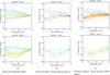 |
Fig. 9 N-band spectra for type 1 objects (top row) and type 2 objects (bottom row). The spectra have been normalized to the 12 μm flux. The colors indicate the slope of the continuum, warm spectra are given. |
7.4. Mid-infrared emission efficiency
In this section we try to find a reasonable estimate of the intrinsic amount of UV flux, emitted by the accretion disk, by using the observed 12 μm nuclear flux and the efficiency ratio ηUV−IR, defined in this case as the ratio between the UV flux and the observed 12 μm flux. For a dusty medium distributed non-uniformly in a volume, the efficiency ratio is no longer constant, but is dependent on the LOS. The variations of the efficiency ratio ηUV−IR depend on the distribution of the medium and in particular become larger when the LOS is optically thick in the infrared, or in other words, when self-absorption of the dust becomes more relevant. The diversity of ηUV−IR values should be kept in consideration when computing the UV luminosity from the observed infrared luminosity in Seyfert galaxies.
To obtain a reasonable estimate of UV flux for our objects, we computed for every best-fit model the distribution of the efficiency factors along multiple line-of-sights and with different realizations. For the type 2 objects we computed the distribution of the efficiency ratio for model B (best type 2 model) reported in Table 3, and then we used the infrared flux to obtained an estimate of the UV emission from the accretion disk. We show the computed UV flux in Fig. 10 together with the corrected 2−10 keV X-ray fluxes.
For the type 1 models we used a slightly different approach. We previously showed that our entire sample of type 1 objects cannot be fit with the same model as the type 2s, but it might be possible that a fraction of our type 1s can be consistent with the unobscured LOS of the type 2 model. For objects where our model B fails in describing the interferometric measurements we seem to find a good fit using a low filling factor environment. For our type 1 objects we individually searched for the best-fit models using a low filling factor between 0.4−1.4% and also a higher filling factor between 5.3−20%. In Fig. 10 we show for every type 1 object two estimates of the UV flux, one using a model with a low filling factor and the second using a high filling factor. For objects that cannot reasonably be described using a high filling factor model, we only show the estimates from the low filling factor model.
Corrected 2−10 keV X-ray luminosities are assumed to be related to the UV bump of the accretion disk and are sometimes used to estimate the UV luminosity. From Fig. 10 we observe that a correlation might exist if we allow a mixture of objects with a low and a high filling factor. It is also clear that our objects with the low filling factor models do not seem to be outliers despite their general low efficiency ratio ηUV−IR.
7.5. Stability of the clouds
Our best-fit low filling factor models are built with a limited number of clouds with high optical depths, typically with τ9.7 ≥ 8. Clouds with such optical depths should be quite massive, therefore the question arises whether these clouds are physically possible. In particular, we investigate if the thermal pressure is sufficient to keep the clouds from collapsing. To answer this question, we used the Jeans instability criterion. From the virial theorem and assuming a static, spherical, homogeneous cloud, we obtain that the critical mass for a cloud to collapse is given by MJ ~ 6.64 × 10²²T3/2ρ− 1/2 [g]. If the mass of our cloud exceeds the value of MJ, the thermal pressure is not enough to keep our cloud from collapsing.
Since for our best type 1 model the clouds are located close to the inner rim, we tested the stability of one such clouds. The typical volume of a cloud close to the inner rim is Vcl = 9.8 × 1053 cm3 and the dust mass of the cloud is Mdust = 0.77 M⊙. To derive the total mass of the cloud we used a dust to gas ratio ρdust/ρgas = 0.01, which gives a total mass of Mtot = 77 M⊙. From the radiative transfer computation we obtain an average temperature of the cloud of T ~ 270 K. The resulting Jeans mass for this configuration is MJ ~ 361 M⊙, which is greater than the total mass of our cloud Mtot = 77 M⊙. Although this calculation does not include other effects, such as rotation or shearing effects, we show that in a static situation the thermal pressure can prevent such clouds from collapsing. In fact, our calculation predicts that the cloud might expand since it is not confined by gravity. It might also be possible that the clouds are confined by external gas pressure.
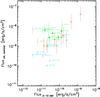 |
Fig. 10 Absorption-corrected 2−10 keV X-ray flux versus nuclear UV flux estimated from models. The symbols indicate the median value for the estimated UV luminosities from their respective best-fit models, and the lines indicate the dispersion (68% area) in the possible values. Type I galaxies that can only be fit with type A models (filling factors 0.4−1.4%) are given as filled circles. Those that can also be fit by type B models (filling factors 5.3−20%) are shown twice, with the model UV-flux values given as triangles (model A) and asterisks (model B). All type 2 galaxies are shown as asterisks. |
8. Conclusions
We presented results from a statistical method developed to interpret interferometric data with complex radiative transfer models. We applied our method to the interferometric data of AGNs published by Burtscher et al. (2013) and constructed our model images according to the dusty torus models from Schartmann et al. (2008). We summarize our major findings below.
-
1.
Mid-infrared interferometric data of a combined AGN sample,including both type 1 and type 2 sources,cannot be described by a single stochastic model (using Schartmannet al. 2008 models) under the assumptionsof the Standard Model where observed differences are only attributed toinclination and line-of-sight effects.
-
2.
Type 1 and type 2 sources can be well explained by such models if they are taken as two separate subsets with different model parameters for each subset. We found that the greatest difference between the models that describe each subset is in the volume fraction that the clouds occupy in the inner regions.
-
3.
Seyfert type 1 galaxies are best explained by using torus models with low filling factors at the inner regions, between 0.4% and 1.5% of the volume of a spherical shell. The low filling factor implies a relatively small number of clouds. This small number produces large apparent fluctuations in interferometric measures of the type 1 sources, including a broad range of apparent geometrical sizes. This agrees with the large dispersion in sizes reported by Burtscher et al. (2013).
-
4.
Seyfert type 2 galaxies are best explained with torus models with a filling factor of 5 or larger than those describing the Seyfert type 1s. The torus emission in the type 2 sources seems to be dominated by the warm infrared emission from a very compact region that escapes through the holes created by the clumpy nature of the torus. These random holes might be causing the asymmetrical emission in the large-scale structure.
-
5.
Although two models are necessary and sufficient to explain our observations of the two Seyfert subsets, this represents an oversimplification. By accidents of obscuration, some of the observed type 1 sources may arise from high filling-factor geometries and some of the type 2 sources from low filling-factor geometries in a more complicated version of the Standard Model. In addition, of course, more than two geometries may actually be present.
-
6.
The reduction of the silicate feature in our models is mostly caused by the large optical depth of the clouds and to a lesser degree to the shielding effect caused by non-silicate grains. For a low number of clouds, the reduction of the silicate feature is not caused by outer clouds blocking our view to the hot surfaces of the inner clouds.
The instrument MIDI is a two-telescope Michelson-type beam combiner with an operational spectral range in the atmospheric N-band (λ ~ 8−13 μm).
A (u,v) point can be defined as the coordinates, for a given projected baseline and a position angle, in the Fourier-transform space of the angular distribution of the source on the sky.
EWS is available for download from http://home.strw.leidenuniv.nl/~jaffe/ews/index.html
Acknowledgments
The authors thank the referee for the thoughtful and helpful comments. We also thank S. Honig, K. Meisenheimer, M. Schartmann, and L. Burtscher for their comments, discussions and help, which all contributed to making this work possible. N. López-Gonzaga was supported by grant 614.000 from the Nederlandse Organisatie voor Wetenschappelijk Onderzoek and acknowledges support from a CONACyT graduate fellowship.
References
- Alonso-Herrero, A., Colina, L., Packham, C., et al. 2006, ApJ, 652, L83 [NASA ADS] [CrossRef] [Google Scholar]
- Alonso-Herrero, A., Ramos Almeida, C., Mason, R., et al. 2011, ApJ, 736, 82 [NASA ADS] [CrossRef] [Google Scholar]
- Antonucci, R. 1993, ARA&A, 31, 473 [Google Scholar]
- Antonucci, R. R. J., & Miller, J. S. 1985, ApJ, 297, 621 [NASA ADS] [CrossRef] [Google Scholar]
- Asmus, D., Gandhi, P., Smette, A., Hönig, S. F., & Duschl, W. J. 2011, A&A, 536, A36 [NASA ADS] [CrossRef] [EDP Sciences] [Google Scholar]
- Asmus, D., Hönig, S. F., Gandhi, P., Smette, A., & Duschl, W. J. 2014, MNRAS, 439, 1648 [NASA ADS] [CrossRef] [Google Scholar]
- Asmus, D., Gandhi, P., Hönig, S. F., Smette, A., & Duschl, W. J. 2015, MNRAS, 454, 766 [NASA ADS] [CrossRef] [Google Scholar]
- Barvainis, R. 1987, ApJ, 320, 537 [NASA ADS] [CrossRef] [Google Scholar]
- Bock, J. J., Neugebauer, G., Matthews, K., et al. 2000, AJ, 120, 2904 [NASA ADS] [CrossRef] [Google Scholar]
- Buchanan, C. L., Gallimore, J. F., O’Dea, C. P., et al. 2006, AJ, 132, 401 [NASA ADS] [CrossRef] [Google Scholar]
- Burtscher, L., Tristram, K. R. W., Jaffe, W. J., & Meisenheimer, K. 2012, in SPIE Conf. Ser., 8445, 84451G [Google Scholar]
- Burtscher, L., Meisenheimer, K., Tristram, K. R. W., et al. 2013, A&A, 558, A149 [NASA ADS] [CrossRef] [EDP Sciences] [Google Scholar]
- Burtscher, L., Orban de Xivry, G., Davies, R. I., et al. 2015, A&A, 578, A47 [NASA ADS] [CrossRef] [EDP Sciences] [Google Scholar]
- Dorodnitsyn, A., Bisnovatyi-Kogan, G. S., & Kallman, T. 2011, ApJ, 741, 29 [NASA ADS] [CrossRef] [Google Scholar]
- Dorodnitsyn, A., Kallman, T., & Proga, D. 2015, 2014 Fermi Symposium proceedings – eConf C14102.1 [arXiv:1502.02383] [Google Scholar]
- Dullemond, C. P., & van Bemmel, I. M. 2005, A&A, 436, 47 [NASA ADS] [CrossRef] [EDP Sciences] [Google Scholar]
- Eisenhauer, F., Perrin, G., Brandner, W., et al. 2011, The Messenger, 143, 16 [NASA ADS] [Google Scholar]
- Elitzur, M. 2012, ApJ, 747, L33 [NASA ADS] [CrossRef] [Google Scholar]
- Elvis, M., Wilkes, B. J., McDowell, J. C., et al. 1994, ApJS, 95, 1 [NASA ADS] [CrossRef] [Google Scholar]
- Feltre, A., Hatziminaoglou, E., Fritz, J., & Franceschini, A. 2012, MNRAS, 426, 120 [NASA ADS] [CrossRef] [Google Scholar]
- Galliano, E., Alloin, D., Pantin, E., Lagage, P. O., & Marco, O. 2005, A&A, 438, 803 [NASA ADS] [CrossRef] [EDP Sciences] [Google Scholar]
- Gandhi, P., Horst, H., Smette, A., et al. 2009, A&A, 502, 457 [NASA ADS] [CrossRef] [EDP Sciences] [Google Scholar]
- Georgantopoulos, I., & Akylas, A. 2010, A&A, 509, A38 [NASA ADS] [CrossRef] [EDP Sciences] [Google Scholar]
- Granato, G. L., & Danese, L. 1994, MNRAS, 268, 235 [NASA ADS] [CrossRef] [Google Scholar]
- Haas, M., Siebenmorgen, R., Pantin, E., et al. 2007, A&A, 473, 369 [NASA ADS] [CrossRef] [EDP Sciences] [Google Scholar]
- Henyey, L. G., & Greenstein, J. L. 1941, ApJ, 93, 70 [NASA ADS] [CrossRef] [Google Scholar]
- Heymann, F., & Siebenmorgen, R. 2012, ApJ, 751, 27 [NASA ADS] [CrossRef] [Google Scholar]
- Hönig, S. F., & Kishimoto, M. 2010, A&A, 523, A27 [NASA ADS] [CrossRef] [EDP Sciences] [Google Scholar]
- Hönig, S. F., Beckert, T., Ohnaka, K., & Weigelt, G. 2006, A&A, 452, 459 [NASA ADS] [CrossRef] [EDP Sciences] [Google Scholar]
- Hönig, S. F., Kishimoto, M., Gandhi, P., et al. 2010, A&A, 515, A23 [NASA ADS] [CrossRef] [EDP Sciences] [Google Scholar]
- Hönig, S. F., Kishimoto, M., Antonucci, R., et al. 2012, ApJ, 755, 149 [NASA ADS] [CrossRef] [Google Scholar]
- Hönig, S. F., Kishimoto, M., Tristram, K. R. W., et al. 2013, ApJ, 771, 87 [NASA ADS] [CrossRef] [Google Scholar]
- Horst, H., Smette, A., Gandhi, P., & Duschl, W. J. 2006, A&A, 457, L17 [NASA ADS] [CrossRef] [EDP Sciences] [Google Scholar]
- Horst, H., Gandhi, P., Smette, A., & Duschl, W. J. 2008, A&A, 479, 389 [NASA ADS] [CrossRef] [EDP Sciences] [Google Scholar]
- Horst, H., Duschl, W. J., Gandhi, P., & Smette, A. 2009, A&A, 495, 137 [NASA ADS] [CrossRef] [EDP Sciences] [Google Scholar]
- Ichikawa, K., Ueda, Y., Terashima, Y., et al. 2012, ApJ, 754, 45 [NASA ADS] [CrossRef] [Google Scholar]
- Ichikawa, K., Packham, C., Ramos Almeida, C., et al. 2015, ApJ, 803, 57 [NASA ADS] [CrossRef] [Google Scholar]
- Kishimoto, M., Hönig, S. F., Tristram, K. R. W., & Weigelt, G. 2009, A&A, 493, L57 [NASA ADS] [CrossRef] [EDP Sciences] [Google Scholar]
- Kishimoto, M., Hönig, S. F., Antonucci, R., et al. 2011a, A&A, 527, A121 [CrossRef] [EDP Sciences] [Google Scholar]
- Kishimoto, M., Hönig, S. F., Antonucci, R., et al. 2011b, A&A, 536, A78 [NASA ADS] [CrossRef] [EDP Sciences] [Google Scholar]
- Krolik, J. H., & Begelman, M. C. 1988, ApJ, 329, 702 [NASA ADS] [CrossRef] [Google Scholar]
- Leinert, C., Graser, U., Przygodda, F., et al. 2003, Ap&SS, 286, 73 [NASA ADS] [CrossRef] [Google Scholar]
- Levenson, N. A., Radomski, J. T., Packham, C., et al. 2009, ApJ, 703, 390 [NASA ADS] [CrossRef] [Google Scholar]
- Lopez, B., Antonelli, P., Wolf, S., et al. 2008, in SPIE Confer. Ser., 7013 [Google Scholar]
- López-Gonzaga, N., Jaffe, W., Burtscher, L., Tristram, K. R. W., & Meisenheimer, K. 2014, A&A, 565, A71 [NASA ADS] [CrossRef] [EDP Sciences] [Google Scholar]
- López-Gonzaga, N., Burtscher, L., Tristram, K. R. W., Meisenheimer, K., & Schartmann, M. 2016, A&A, 591, A47 [NASA ADS] [CrossRef] [EDP Sciences] [Google Scholar]
- Lutz, D., Maiolino, R., Spoon, H. W. W., & Moorwood, A. F. M. 2004, A&A, 418, 465 [NASA ADS] [CrossRef] [EDP Sciences] [Google Scholar]
- Manske, V., Henning, T., & Men’shchikov, A. B. 1998, A&A, 331, 52 [NASA ADS] [Google Scholar]
- Mason, R. E., Lopez-Rodriguez, E., Packham, C., et al. 2012, AJ, 144, 11 [NASA ADS] [CrossRef] [Google Scholar]
- Mateos, S., Carrera, F. J., Alonso-Herrero, A., et al. 2016, ApJ, 819, 166 [NASA ADS] [CrossRef] [Google Scholar]
- Mathis, J. S., Rumpl, W., & Nordsieck, K. H. 1977, ApJ, 217, 425 [NASA ADS] [CrossRef] [Google Scholar]
- Meisenheimer, K., Tristram, K. R. W., Jaffe, W., et al. 2007, A&A, 471, 453 [NASA ADS] [CrossRef] [EDP Sciences] [Google Scholar]
- Mor, R., Netzer, H., & Elitzur, M. 2009, ApJ, 705, 298 [NASA ADS] [CrossRef] [Google Scholar]
- Nenkova, M., Ivezić, Ž., & Elitzur, M. 2002, ApJ, 570, L9 [NASA ADS] [CrossRef] [Google Scholar]
- Nenkova, M., Sirocky, M. M., Ivezić, Ž., & Elitzur, M. 2008a, ApJ, 685, 147 [NASA ADS] [CrossRef] [Google Scholar]
- Nenkova, M., Sirocky, M. M., Nikutta, R., Ivezić, Ž., & Elitzur, M. 2008b, ApJ, 685, 160 [NASA ADS] [CrossRef] [Google Scholar]
- Neugebauer, G., Oke, J. B., Becklin, E. E., & Matthews, K. 1979, ApJ, 230, 79 [NASA ADS] [CrossRef] [Google Scholar]
- Nikutta, R., Elitzur, M., & Lacy, M. 2009, ApJ, 707, 1550 [NASA ADS] [CrossRef] [Google Scholar]
- Packham, C., Radomski, J. T., Roche, P. F., et al. 2005, ApJ, 618, L17 [NASA ADS] [CrossRef] [Google Scholar]
- Pier, E. A., & Krolik, J. H. 1992, ApJ, 401, 99 [NASA ADS] [CrossRef] [Google Scholar]
- Pier, E. A., & Krolik, J. H. 1993, ApJ, 418, 673 [NASA ADS] [CrossRef] [Google Scholar]
- Raban, D., Jaffe, W., Röttgering, H., Meisenheimer, K., & Tristram, K. R. W. 2009, MNRAS, 394, 1325 [NASA ADS] [CrossRef] [Google Scholar]
- Ramos Almeida, C., Levenson, N. A., Rodríguez Espinosa, J. M., et al. 2009, ApJ, 702, 1127 [NASA ADS] [CrossRef] [Google Scholar]
- Ramos Almeida, C., Levenson, N. A., Alonso-Herrero, A., et al. 2011, ApJ, 731, 92 [NASA ADS] [CrossRef] [Google Scholar]
- Reunanen, J., Prieto, M. A., & Siebenmorgen, R. 2010, MNRAS, 402, 879 [NASA ADS] [CrossRef] [Google Scholar]
- Sanders, D. B., Phinney, E. S., Neugebauer, G., Soifer, B. T., & Matthews, K. 1989, ApJ, 347, 29 [NASA ADS] [CrossRef] [Google Scholar]
- Schartmann, M., Meisenheimer, K., Camenzind, M., et al. 2008, A&A, 482, 67 [NASA ADS] [CrossRef] [EDP Sciences] [Google Scholar]
- Schartmann, M., Wada, K., Prieto, M. A., Burkert, A., & Tristram, K. R. W. 2014, MNRAS, 445, 3878 [NASA ADS] [CrossRef] [Google Scholar]
- Siebenmorgen, R., Haas, M., Pantin, E., et al. 2008, A&A, 488, 83 [NASA ADS] [CrossRef] [EDP Sciences] [Google Scholar]
- Siebenmorgen, R., Heymann, F., & Efstathiou, A. 2015, A&A, 583, A120 [NASA ADS] [CrossRef] [EDP Sciences] [Google Scholar]
- Stalevski, M., Fritz, J., Baes, M., Nakos, T., & Popović, L. Č. 2012, MNRAS, 420, 2756 [NASA ADS] [CrossRef] [Google Scholar]
- Stern, D. 2015, ApJ, 807, 129 [NASA ADS] [CrossRef] [Google Scholar]
- Suganuma, M., Yoshii, Y., Kobayashi, Y., et al. 2006, ApJ, 639, 46 [NASA ADS] [CrossRef] [Google Scholar]
- Tomono, D., Doi, Y., Usuda, T., & Nishimura, T. 2001, ApJ, 557, 637 [NASA ADS] [CrossRef] [Google Scholar]
- Tristram, K. R. W., & Schartmann, M. 2011, A&A, 531, A99 [NASA ADS] [CrossRef] [EDP Sciences] [Google Scholar]
- Tristram, K. R. W., Burtscher, L., Jaffe, W., et al. 2014, A&A, 563, A82 [NASA ADS] [CrossRef] [EDP Sciences] [Google Scholar]
- Urry, C. M., & Padovani, P. 1995, PASP, 107, 803 [NASA ADS] [CrossRef] [Google Scholar]
- van der Wolk, G., Barthel, P. D., Peletier, R. F., & Pel, J. W. 2010, A&A, 511, A64 [NASA ADS] [CrossRef] [EDP Sciences] [Google Scholar]
- Wada, K. 2012, ApJ, 758, 66 [NASA ADS] [CrossRef] [Google Scholar]
- Weigelt, G., Hofmann, K.-H., Kishimoto, M., et al. 2012, A&A, 541, L9 [NASA ADS] [CrossRef] [EDP Sciences] [Google Scholar]
Appendix A: Model setup
The models used for our database of infrared images are built based on the approach described by (Schartmann et al. 2008). These wedge-like clumpy torus models are one of many different torus models currently available, but their main advantage is that it is relatively easy to proceed from a model with only a few clouds to models with a large number of clouds that resemble the smooth distribution of continuous models better.
The models are built using spherical coordinates. The dust-free volume is defined by the half-opening angle θop, where clouds are only allowed to exist within the region of θop<θ<π−θop. The cloud centers are distributed in equal volumes randomly along the azimuthal direction and polar angle in the allowed zone. The radial position of the clouds are randomly distributed and follow a power-law density profile ρr = ρ0(r/ 1 pc)α, where α is the density profile index and ρ0 a normalization constant.
Dust clouds are spherical, homogeneously filled with dust, and all possess the same optical depth. The radius of the clouds is proportional to their radial position acl = a0(r/ 1 pc), where a0 is a constant value. The number of clouds of the model is determined by the filling factor. We define the filling factor as the ratio between the volume occupied by the clouds and the total volume of a spherical shell defined by the inner radius of the model and the radius at 1 pc. Finally, the total amount of dust in the model is determined by normalizing the total density in order to obtain a fixed average optical depth at 9.7 μm along the equatorial plane.
Since the true mixture of grains in AGNs is not fully determined, we use a typical mixture of dust grains for the intrastellar medium, consisting of 62.5% silicates and 37.5% of graphites, where the percentages correspond to the mass fraction. In the case of the graphites, we take two different sets of optical constants: one third of our graphites is represented by graphites whose electric field vector oscillates in parallel to the crystal axis of the grain, and two thirds of the grains have a perpendicular oscillation. For the size distribution we use the classic MRN-model (Mathis et al. 1977). Following Schartmann et al. (2008), we use a decoupled computation of the temperature for each dust species and grain size. For each dust species we take five bins of different sizes, so we take in total 15 different dust density grids as input. Since the treatment of the dust temperature is decoupled for each grain size, we also implement the sublimation temperature of each grain type. We take a sublimation temperature of 1500 K for the graphites and 1000 K for the silicates.
To approximate the SED of the accretion disk, we use a broken power-law spectrum as described by Hönig et al. (2006), which is derived from quasi-stellar object spectra (Manske et al. 1998):  (A.1)
(A.1)
Appendix B: Scaling of the observables
Our procedure for stochastically simulating a specific observation according to a specific set of model parameters is the following:
-
1.
Choose a random cloud realization in accordance with the modelparameters. Choose also an inclination angle θ and rotation angle φ on the sky.
-
2.
Given the nominal model luminosity Lm, compute the cloud temperature distribution and three-dimensional radiation field.
-
3.
Using θ and φ, project the emitted radiation at the three chosen wavelengths onto a plane with these inclination and rotation angles at the nominal distance Dm. Take the two-dimensional Fourier transform of these images to evaluate the model-correlated fluxes at all baselines BLm. Evaluate especially the total zero-baseline 12 μm flux density fm(12) and also determine from the optical depth in the visual τV whether this realization would be classified as type 1 or 2.
-
4.
Now consider each actually observed galaxy in the sample, with its actual observed values of Ds and fs(12). If it is the incorrect Seyfert type, skip this realization. Otherwise:
-
5.
Move the model from Dm to Ds. This rescales all model apparent fluxes by (Dm/Ds)2 and all angular sizes by Dm/Ds.
-
6.
Adjust Lm to bring the scaled value of fm(12) to equal the observed fs(12); this rescales all angular sizes in proportion to
 . The net effect of operations (5) and (6) is to multiply all the original model fluxes by ϵ, the ratio of fs(12) to the original value of fm(12), and all angular sizes by the
  .
. -
7.
For each observed baseline BLs, look up the correlated flux in the 2D transform of the unscaled model at baseline length
 (to account for the rescaled angular size) and multiply this value by ϵ (to account for the rescaled fluxes). This flux value can now be directly compared to the measured correlated flux at BLs.
 -
8.
Repeat these steps for each cloud realization and for all the chosen values of θ and φ. The set of all the correlated fluxes for a given baseline represents the expected distribution of measured fluxes under the assumption of random distributions of these stochastic variables.
Appendix C: Correlation losses
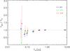 |
Fig. C.1 Average fraction of the recovered flux Fout and the input flux Fin as a function of the input flux for our dilution experiment at different wavelengths (8.5 μm, 10.0 μm, and 12.0 μm). For each value of Fin the symbols for the three wavelengths have been shifted slightly for better readability. The average values were computed from the output fluxes obtained from 76 calibrators, and the errorbars represent standard deviation of the output fluxes. |
The atmospheric phase jitter might lead to a reduction of the estimated correlated flux in our measurements. To estimate the amount of correlation losses caused during data reduction, we used a similar strategy as explained by Burtscher et al. (2012). We simulated an observation of a weak target with a known flux to observe the difference between the input and the output flux. Since the data used for this work were reduced using EWS 2.04 and the dilution experiment previously reported by Burtscher et al. (2012) was done using the EWS snapshot version 2012 January 25, we repeated this experiment with the updated version to determine possible changes. For our experiment, we took the raw data of a bright target with known flux, a calibrator in our case, multiplied the input flux by a factor f< 1 and added artificial noise to the data. After performing this process several times, we obtained an estimate of the amount of losses in the flux due to correlation losses.
We performed this dilution experiment with 76 calibrators observed in different nights and diluted to simulate weak targets with 50−8000 mJy of correlated flux. The losses relative to the highest flux (8 Jy) were determined at three wavelengths of 8.5, 10.0, and 12.0 μm. Figure C.1 shows the losses at these three wavelengths, and for the weak sources with fluxes <400 mJy these losses clearly become more significant at the short wavelength range (closer to 8 μm), while the losses are moderate above the 12 μm. We used this information to correct the average correlated fluxes of the sources for this work. For the source with high correlation losses we took the average correlated flux obtained after the data reduction and multiplied it by the decorrelation correction factor obtained from our dilution experiment.
Appendix D: Dust sublimation
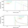 |
Fig. D.1 Temperatures for the three smallest grain sizes of each species in a shell with a radial optical thickness of τ9.7 = 10-4 (top) and τ = 8 (bottom). The colors indicate the different species of grains: blue – graphites ⊥, green – graphites ||, and red – silicates. |
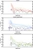 |
Fig. D.2 Convergence of the temperature for the three smallest grains. Each line indicate the relative difference after each iteration. The darker the color, the higher the number of iterations. |
The radiative transfer code RADMC-3D does not include an internal computation to account for dust sublimation. To include dust sublimation in our models, we slightly modified the code. Each time a photon package enters a cell, it increases the energy of the cell and thus increases the temperature of the dust of this cell. When the dust in the cells exceeds the dust sublimation temperature, the dust inside the cell is completely removed. To accurately estimate the temperature of the system using dust sublimation, we performed an iterative process for which the code several times computed the temperatures and removed the corresponding cells. When the differences between different iterations were below a certain tolerance (we took a value of 5%), we performed a last computation without removing any dust in the cells to ensure the conservation of energy in the system. To show how our implementation of the dust sublimation works in different situations we show examples of an optically thick and optically thin case. In Fig. D.1 we show the temperature of the three smallest grains of each species for a spherical shell with τ9.7 = 10-4 and τ9.7 = 8, respectively. Both shells have an initial inner radius of 0.3 pc and an outer radius of 5 pc. We can observe clearly that in the optically thick case, the temperature rises more quickly and the sublimation radius for the three species are closer than in the optically thin case. We made sure that we had enough cells close to the inner radius to obtain an accurate solution. In Fig. D.2, we show for the optically thick case, the relative differences between each iteration and our final computation. After a few iterations, the temperature in every cell reaches a relative difference below our tolerance value.
Appendix E: Acceptance levels
For our method we used linear transformations computed for each model to remove the mean values, normalize the variance, and remove correlations. We expect that if our models agree with the observational data, the final distribution of the data points have a zero mean and variance equal to one. To test if this is true for every model, we applied a χ2-test to the sample mean (μ) and sample variance (s2) of the normalized measurements, 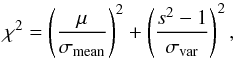 (E.1)where σmean and σvar are the computed variance for the sample mean and the sample variance, respectively. These two quantities were computed from the distributions of each model. Although the distribution produced by our models might not be Gaussian distributions, when we combine all of the measurements to compute the final quantities, the resulting distribution should be more less similar to a Gaussian distribution, according to the central limit theorem. Therefore, we used the probability values assigned for the χ2-distribution to derive the level of acceptance for each model.
To test if our assumptions are valid, we performed a consistency test. We took a particular model and created 200 samples with measurements of 20 simulated objects using sparse (u,v) coverages and simulating uncertainties of 10%. For each sample we applied our test with the model that was used to create the simulated samples. In Fig. E.1 we show the distribution of the sample mean and variance for all the samples. We also show that we can safely build our confidence intervals assuming the probabilities for a normal distribution.
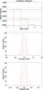 |
Fig. E.1 Top: histogram showing the frequency of our sample in terms of the σ areas. The lines indicate the 68% and 27.5%, respectively. The dashed lines give the expected uncertainty for 200 experiments. Center and bottom: histogram of the sample mean and variance of the normalized measurements for the 200 experiments. |
All Tables
All Figures
|
Fig. 1 Absorption-corrected 2−10 keV X-ray fluxes versus nuclear 12 μm fluxes. |
| In the text | |
|
Fig. 2 Discrete maps showing the level of acceptance around the best-fit solution for type 1 sources (first and second column) and type 2 sources (second and third column). In every panel, three of the five parameters of the best solution are kept fixed, while the two parameters shown in the labels of each plot are explored. The best-fit solution is shown with an asterisk. The color of the squares indicates the acceptance value of the parameters based on a χ2-test. The blue squares indicate the probability of the χ2-value using the equivalent percentages of a Gaussian distribution at the 1σ level (68%), green the probability at 95% confidence, yellow up to 99.5% and red above 99.5%. |
| In the text | |
|
Fig. 3 Comparison of the discrete maps for models of type 2s using (left) no luminosity reweighting and (right) a more realistic reweighting with γ = 1. |
| In the text | |
|
Fig. 4 Left: 12 μm interferometric visibilities of type 1 (top) and type 2 sources (bottom) plotted against the normalized projected baseline. For every object we include visibilities for two different position angles connected by independent lines. The normalized baseline is scaled from the observed baseline for each source to normalize its single-aperture 12 μm flux; cf. Sect. 4.1. Each symbol indicates the longest baseline data point available at the given position angle for an individual object. The color of the symbols indicates the value of the infrared luminosity of the source as shown on the scale at the right, data are from by Table 1. Top right: model normalized 12 μm interferometric radial plots for various lines of sight where the nucleus is exposed, corresponding to type 1 objects, computed from type A models (blue) and from type B models (red). Bottom right: model radial plots for various obscured LOS, corresponding to type 2 objects, computed for the best type B models. |
| In the text | |
|
Fig. 5 12 μm images created from one of the best type 1 models (model A). We only show lines-of-sight where the nucleus is exposed. Each plot shows a different realization of the cloud positions. Labels denote the distance to the center in pc. |
| In the text | |
|
Fig. 6 Same as Fig. 5, but the images are created from the unobscured lines-of-sight from model B, i.e., type 1s with the same filling factor as type 2 objects. |
| In the text | |
|
Fig. 7 Same as Fig. 5, but the images are created from the obscured lines-of-sight from model B, i.e., the best type 2 model. |
| In the text | |
|
Fig. 8 SEDs for multiple realizations of the best-fit model. |
| In the text | |
|
Fig. 9 N-band spectra for type 1 objects (top row) and type 2 objects (bottom row). The spectra have been normalized to the 12 μm flux. The colors indicate the slope of the continuum, warm spectra are given. |
| In the text | |
|
Fig. 10 Absorption-corrected 2−10 keV X-ray flux versus nuclear UV flux estimated from models. The symbols indicate the median value for the estimated UV luminosities from their respective best-fit models, and the lines indicate the dispersion (68% area) in the possible values. Type I galaxies that can only be fit with type A models (filling factors 0.4−1.4%) are given as filled circles. Those that can also be fit by type B models (filling factors 5.3−20%) are shown twice, with the model UV-flux values given as triangles (model A) and asterisks (model B). All type 2 galaxies are shown as asterisks. |
| In the text | |
|
Fig. C.1 Average fraction of the recovered flux Fout and the input flux Fin as a function of the input flux for our dilution experiment at different wavelengths (8.5 μm, 10.0 μm, and 12.0 μm). For each value of Fin the symbols for the three wavelengths have been shifted slightly for better readability. The average values were computed from the output fluxes obtained from 76 calibrators, and the errorbars represent standard deviation of the output fluxes. |
| In the text | |
|
Fig. D.1 Temperatures for the three smallest grain sizes of each species in a shell with a radial optical thickness of τ9.7 = 10-4 (top) and τ = 8 (bottom). The colors indicate the different species of grains: blue – graphites ⊥, green – graphites ||, and red – silicates. |
| In the text | |
|
Fig. D.2 Convergence of the temperature for the three smallest grains. Each line indicate the relative difference after each iteration. The darker the color, the higher the number of iterations. |
| In the text | |
|
Fig. E.1 Top: histogram showing the frequency of our sample in terms of the σ areas. The lines indicate the 68% and 27.5%, respectively. The dashed lines give the expected uncertainty for 200 experiments. Center and bottom: histogram of the sample mean and variance of the normalized measurements for the 200 experiments. |
| In the text | |
Current usage metrics show cumulative count of Article Views (full-text article views including HTML views, PDF and ePub downloads, according to the available data) and Abstracts Views on Vision4Press platform.
Data correspond to usage on the plateform after 2015. The current usage metrics is available 48-96 hours after online publication and is updated daily on week days.
Initial download of the metrics may take a while.