| Issue |
A&A
Volume 590, June 2016
|
|
|---|---|---|
| Article Number | A75 | |
| Number of page(s) | 17 | |
| Section | Interstellar and circumstellar matter | |
| DOI | https://doi.org/10.1051/0004-6361/201424385 | |
| Published online | 13 May 2016 | |
Structure and stability in TMC-1: Analysis of NH3 molecular line and Herschel continuum data
1
Eötvös Loránd UniversityDepartment of Astronomy,
Pázmány Péter sétány 1/A,
1117
Budapest,
Hungary
e-mail:
feher.orsolya@csfk.mta.hu
2
Konkoly Observatory, Research Centre for Astronomy and Earth
Sciences, Hungarian Academy of Sciences, Konkoly Thege Miklós út 15-17, 1121
Budapest,
Hungary
3
Jeremiah Horrocks Institute, University of Central
Lancashire, Preston
PR1 2HE,
UK
4
Max Planck Institute for Radioastronomy,
Auf dem Hügel 69, 53121
Bonn,
Germany
5
Department of Physics, PO Box 64, University of
Helsinki, 00014
Helsinki,
Finland
6
European Southern Observatory, Karl-Schwarzschild-Str. 2, 85748
Garching bei München,
Germany
Received: 12 June 2014
Accepted: 11 March 2016
Aims. We examined the velocity, density, and temperature structure of Taurus molecular cloud-1 (TMC-1), a filamentary cloud in a nearby quiescent star forming area, to understand its morphology and evolution.
Methods. We observed high signal-to-noise (S/N), high velocity resolution NH3(1,1), and (2, 2) emission on an extended map. By fitting multiple hyperfine-split line profiles to the NH3(1, 1) spectra, we derived the velocity distribution of the line components and calculated gas parameters on several positions. Herschel SPIRE far-infrared continuum observations were reduced and used to calculate the physical parameters of the Planck Galactic Cold Clumps (PGCCs) in the region, including the two in TMC-1. The morphology of TMC-1 was investigated with several types of clustering methods in the parameter space consisting of position, velocity, and column density.
Results. Our Herschel-based column density map shows a main ridge with two local maxima and a separated peak to the south-west. The H2 column densities and dust colour temperatures are in the range of 0.5−3.3 × 1022 cm-2 and 10.5−12 K, respectively. The NH3 column densities and H2 volume densities are in the range of 2.8−14.2 × 1014 cm-2 and 0.4−2.8 × 104 cm-3. Kinetic temperatures are typically very low with a minimum of 9 K at the maximum NH3 and H2 column density region. The kinetic temperature maximum was found at the protostar IRAS 04381+2540 with a value of 13.7 K. The kinetic temperatures vary similarly to the colour temperatures in spite of the fact that densities are lower than the critical density for coupling between the gas and dust phase. The k-means clustering method separated four sub-filaments in TMC-1 with masses of 32.5, 19.6, 28.9, and 45.9 M⊙ and low turbulent velocity dispersion in the range of 0.13−0.2 km s-1.
Conclusions. The main ridge of TMC-1 is composed of four sub-filaments that are close to gravitational equilibrium. We label these TMC-1F1 through F4. The sub-filaments TMC-1F1, TMC-1F2, and TMC-1F4 are very elongated, dense, and cold. TMC-1F3 is a little less elongated and somewhat warmer, and probably heated by the Class I protostar, IRAS 04381+2540, which is embedded in it. TMC-1F3 is approximately 0.1 pc behind TMC1-F1. Because of its structure, TMC-1 is a good target to test filament evolution scenarios.
Key words: molecular data / ISM: clouds / ISM: molecules / ISM: abundances / ISM: kinematics and dynamics / radio lines: ISM
© ESO, 2016
1. Introduction
Large-scale filaments have long been recognized as fundamental environments of the star forming process. Several studies revealed that filaments are common structures in interstellar clouds that are populated by young stars in different stages of formation (Schneider & Elmegreen 1979; Bally et al. 1987; Hatchell et al. 2005; Goldsmith et al. 2008). Recent results based on Herschel far-infrared (FIR) observations of nearby star forming regions has once again directed attention to the connection between filaments, dense cores, and stars (see e.g. André et al. 2010). Since star formation occurs mostly in prominent filaments, characterizing the physical properties of these regions is the key to understand the process of star formation.
Properties of the PGCCs in HCL 2.
The Taurus molecular cloud (TMC) is one of the closest, low-mass star forming regions at 140 pc (Elias 1978; Onishi et al. 2002). It was a target of several cloud evolution and star formation studies (Ungerechts & Thaddeus 1987; Mizuno et al. 1995; Goldsmith et al. 2008) and was mapped extensively in CO (Ungerechts & Thaddeus 1987; Onishi et al. 1996; Narayanan et al. 2008) and extinction (Cambrésy 1999; Padoan et al. 2002; Dobashi et al. 2005). The most massive molecular cloud in Taurus is the Heiles cloud 2 (HCL 2; Heiles 1968; Onishi et al. 1996; Tóth et al. 2004), which is the second brightest source on the 353, 545, and 857 GHz Planck maps (Tauber et al. 2010; Planck Collaboration I 2011) in Taurus with a flux density peak in HCL 2B (Heiles 1968).
There are 406 Planck Galactic Cold Clumps (PGCCs) in the Taurus region (Planck Collaboration XXVIII 2016). These are clustered and form 76 groups as was found by Tóth et al. (2016) via the Minimum Spanning Tree method (Planck Collaboration XXIII 2011). One of the largest PGCC groups is HCL 2 with 14 cold clumps; their parameters are listed in Table 1. The clump temperatures and densities were derived from Herschel maps (see Sect. 2.4). The structure of the PGCC group is shown in Fig. 1, which also serves as a finding chart for the parts of HCL 2.
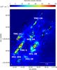 |
Fig. 1 Herschel N(H2) column density map of HCL 2 and the main parts of the cloud. PGCCs with flux quality of 1 and 2 are plotted with black ellipses and the numbers refer to Table 1, which lists the properties of the PGCCs. |
Molecular emission maps show the south-eastern region of HCL 2 as a ring-like structure called the Taurus molecular ring (TMR; Schloerb & Snell 1984). TMC-1 appears as a dense, narrow ridge at the eastern edge of TMR. Two PGCCs are found in this region almost parallel with the galactic plane. Radio spectroscopic surveys indicated a considerable variation in the relative abundance of gas phase molecules, e.g. well-separated cyanopolyyne, ammonia (Little et al. 1979), and SO (Pratap et al. 1997) peaks (see also Table 1). Studies of NH3, HCnN (n = 3, 5, 7), C4H, CS, C34S, HCS+ (Tölle et al. 1981; Gaida et al. 1984; Olano et al. 1988; Hirahara et al. 1992), CH (Suutarinen et al. 2011; Sakai et al. 2012), and other carbon-chain and sulfur-containing molecules (Langer et al. 1995; Pratap et al. 1997) show complex velocity and chemical structure in TMC-1. Hirahara et al. (1992) suggested that the displacement of the column density peaks of carbon-chain and nitrogen bearing molecules is due to different evolutionary states of the regions. The molecular abundances in TMC-1 were modelled by McElroy et al. (2013) using the fifth release of the UMIST Database for Astrochemistry.
The morphologic and evolutionary connection between TMC-1 and HCL 2 was described by Schloerb et al. (1983) and Schloerb & Snell (1984) as TMC-1 being a collapsing, fragmented part of a torus shaped cloud structure (TMR). Cernicharo & Guelin (1987) considered TMC-1 a clump inside a thick, bent filamentary complex projecting itself as a loop on the plane of the sky. The existence and relative motion of fragments in TMC-1 were discussed in various papers (Snell et al. 1982; Schloerb et al. 1983; Olano et al. 1988; Hirahara et al. 1992; Langer et al. 1995; Pratap et al. 1997). Nutter et al. (2008) concluded that in sub-millimeter and FIR, TMR is composed of a dense filament on one side (TMC-1) and a series of point-like sources on the other. High spatial resolution Herschel (Pilbratt et al. 2010) observations resolved the cold clumps found by Planck and in those observations the physical characteristics of the clumps could be determined. Malinen et al. (2012) identified two long filaments in HCL 2 based on near-IR (NIR) extinction and Herschel data; one of these filaments was TMC-1. These authors fitted the column density perpendicular to the filament with a Plummer-like profile and derived an average width of 0.1 pc, which is typical of star forming filaments.
In this paper we discuss the substructures of TMC-1 using our high signal-to-noise ratio (S/N) NH3(1, 1), NH3(2, 2) line observations, and high resolution Herschel FIR maps. We examine the possibility that overlapping sub-filaments are present inside the cloud by partitioning it using various clustering methods in the derived parameter space. We reveal the morphology of TMC-1 and assess the physical state and stability of the different cloud parts.
2. Observations and data reduction
2.1. NH3 observations
The observations of the NH3(J,K) = (1, 1) and (2, 2) inversion transitions were carried out with the Effelsberg 100-m telescope1 during November 21−30, 2008, April 8−13, 2015 and September 10, 2015. The map was obtained in raster mode, which was a number of targeted observations on a grid with a spacing of 40″ (0.027 pc at the distance of TMC-1) with a velocity resolution of 0.038 km s-1. The (0, 0) position of the spectral grid was α(2000) = 04:41:42.5, δ(2000) = 25:41:27. The spectra from 2008 were observed in both position switching (PSW) and frequency switching (FSW) modes; both lines and polarizations were measured simultaneously. In the dataset from 2008, 44% of the spectra were PSW and 56% FSW, and the frequency throw of the FSW observations was 5 MHz. After folding and baseline subtraction of the FSW spectra, the FSW and PSW observations were averaged together weighted by noise. The spectra from 2015 were measured only in FSW mode with a frequency throw of 6 MHz. The pointing errors are within 5−10″ for both datasets. We observed a total of 258 positions with a typical integration time of 4 minutes; a sample spectrum is shown in Fig. 2.
The observing sessions started by measuring the continuum emission of calibration sources (NGC 7027, W3OH). Pointing measurements towards a source close to the target were repeated at least once per hour. For the observations from 2008 NGC 7027 was used for flux calibration with an assumed flux density of 5.51 Jy (Zijlstra et al. 2008). With the average beam size of 37.1″ of the receiver this is equivalent to a main beam brightness temperature TMB = 8.7 K. We calibrated the dependent atmospheric and instrumental gain and efficiency to the elevation with a quadratic function, which was calculated from observing NGC 7027 at different elevations during the observing sessions. The calibration of the 2008 dataset is estimated to be accurate to ±15%.
The data from 2015 was observed with a different receiver (the secondary focus system instead of the prime focus K-band receiver used in 2008), which had an average beam size of 36.6″. The flux calibrator was NGC 7027 again, but since a planetary nebula expands adiabatically, its flux density decreases. According to the model by Zijlstra et al. (2008), the flux density of NGC 7027 was ≈5.46 Jy in 2015. This gives TMB = 8.8 K, which was used to calibrate the 2015 dataset. The spectra on the positions observed in both 2008 and 2015 have an ≈10% difference in intensity, resulting in a 15% accuracy of the merged dataset. The data were reduced and further analysed with the software packages CLASS and GREG2. The calibrated spectra have a typical rms noise of 0.15 K. NH3(1, 1) was detected with S/N> 3 on 171 positions and the NH3(2, 2) line was detected with S/N> 3 on 17 positions. The given line temperatures in this paper are in TMB.
2.2. Separating NH3(1, 1) velocity components
In order to discern the different velocity components in the NH3(1, 1) data, instead of fitting one hyperfine-split (HFS) line profile, we analysed the spectra as follows. We first fitted a single HFS line profile, subtracted it, and then searched the residual for a second component with S/N> 3. This line was also fitted with a HFS line profile. Since in some cases the HFS structure of the secondary components were not detected and the τ(1, 1) optical depth could not be determined well, the vLSR line velocity in the local standard rest frame and the peak TMB values from this fit were verified with a Gaussian profile fit. We then simultaneously fitted both the primary and secondary components with HFS line profiles on the original spectra. During this final fit the software CLASS required initial line parameters for both lines: TMB(1, 1), vLSR, τ(1, 1), and Δv linewidth. For the primary component the initial parameters were the results of the single HFS line profile fit, and for the secondary component vLSR and Δv were taken from the HFS line profile fit of the line on the residual, TMB(1, 1) from the Gaussian fit, and the initial optical depth was 1. None of these parameters were fixed during the simultaneous HFS profile fit. See Fig. 4, which demonstrates this process. We note that line components were not discernible on any of the NH3(2, 2) spectra.
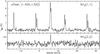 |
Fig. 2 Typical NH3(1, 1) and NH3(2, 2) spectra on our NH3 grid. This position has the highest NH3(1, 1) optical depth from the spectra where we observed the NH3(2, 2) line as well (position #5 in Table 2). |
Fitting a single HFS line profile to potentially multiple line components during the first step can be misleading, since to minimize the residual, the fitting process broadens the resulting line. In case the second component can be found on the residual, we can fit the original spectra again, using two components. However, if the secondary component is blended sufficiently and does not appear on the residual, a single HFS line profile fit is able to reproduce the line but gives false line parameters. This appears as an uncertainty in our calculations, however, the results are more precise where we identify the secondary component. This way we avoid the detection of a fake NH3(1, 1) maximum and get a more detailed picture of the velocity structure.
We examined the minimum separation of the two line components where it is still possible to identify the weaker line component on the residual. The NH3(1, 1) line with the smallest observed linewidth was added to an example spectra while its intensity and their channel separation varied, and then we proceeded to search these spectra for the secondary component with our method. With a channel width of 0.08 km s-1 and rms noise in the range of 0.1−0.3 K, we can only identify the secondary line component with a channel separation of three channels (0.24 km s-1) if its intensity is greater than 50% of the primary component. With a channel separation of four channels (0.32 km s-1), the secondary line with 30% of the primary line component intensity can already be identified. The intensities of the detected secondary components were between 10% and 40% of the primary component with velocity separations of about 0.08 km s-1. Since we fitted both components with HFS line profiles and the separation of the two lines is always greater than the HFS linewidths, it is possible to detect close lines in a few cases.
2.3. Gas parameter calculations from NH3 observations
When calculating gas temperatures and densities from the spectra, the primary (or if no secondary component was identified, the only) NH3(1, 1) line component was used along with the NH3(2, 2) line on the positions where the (2, 2) line was detected with S/N> 3. We fitted the primary NH3(1, 1) components with Gaussian functions to obtain TMB(1, 1) and with HFS line profiles to get τ(1, 1), vLSR and Δv. The NH3(2, 2) lines were fitted with Gaussian functions to obtain their peak main beam brightness temperatures, TMB(2, 2).
The calculations were carried out following Ho & Townes (1983), Ungerechts et al. (1986), and Harju et al. (1993). The Trot rotation temperature of NH3 was calculated with 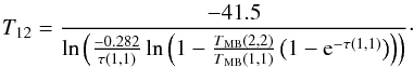 (1)The Tex excitation temperature of the NH3(1, 1) transition was derived from
 ![\begin{equation} T\mathrm{_{MB}}(1, 1)=\frac{h\nu_{11}}{k}[F(T\mathrm{_{ex}})-F(T\mathrm{_{bg}})]\left(1-{\rm e}^{\tau(1, 1)}\right) , \end{equation}](/articles/aa/full_html/2016/06/aa24385-14/aa24385-14-eq53.png) (2)where ν11 is the frequency of the (1, 1) transition, Tbg is the cosmic background temperature (2.726 K), F(T) = 1/(ehν11/kT − 1), and we assume a beam filling factor of 1 since the source is a nearby, extended cloud. We calculated the column density of the ammonia molecules in the upper transition level with
(2)where ν11 is the frequency of the (1, 1) transition, Tbg is the cosmic background temperature (2.726 K), F(T) = 1/(ehν11/kT − 1), and we assume a beam filling factor of 1 since the source is a nearby, extended cloud. We calculated the column density of the ammonia molecules in the upper transition level with 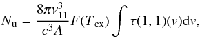 (3)where A is the Einstein coefficient of the NH3(1, 1) transition (1.7 × 10⁻⁷s-1). Assuming a Gaussian line profile and integrating τ over the main line group we can write the integral as
  (4)The N(NH3(1, 1)) total column density of the NH3 molecules in the (1, 1) state is
  (5)Ammonia has two distinct species, the ortho-NH3 (K = 3n) and the para-NH3 (K ≠ 3n), which arise from different relative orientations of the three hydrogen spins. Since the higher energy levels are by orders of magnitude less populated on temperatures around 10 K, we may estimate the Np(NH3) para-NH3 column density from the observed (1, 1) and (2, 2) transitions with
  (6)The Tkin kinetic temperature of the gas was calculated with the half-empiric equation from Tafalla et al. (2004) as follows:
  (7)The n(H2) local molecular hydrogen volume density was estimated using the equation from Ho & Townes (1983) as follows:
 ![\begin{equation} n({\rm H}_2)=\frac{A}{C}\frac{F(T\mathrm{_{ex}})-F(T\mathrm{_{bg}})}{F(T\mathrm{_{kin}})-F(T\mathrm{_{ex}})}[1+F(T\mathrm{_{kin}})] , \end{equation}](/articles/aa/full_html/2016/06/aa24385-14/aa24385-14-eq70.png) (8)where C is the collisional de-excitation rate (8.5 × 10⁻¹¹ cm3 s-1) from Danby et al. (1988).
(8)where C is the collisional de-excitation rate (8.5 × 10⁻¹¹ cm3 s-1) from Danby et al. (1988).
We calculated Np(NH3) upper limits from the secondary NH3(1, 1) line components at each of the 31 positions where those were detected (see Fig. 5 and Appendix B). Based on the HFS line profile fits, on 82 positions the τ(1, 1) optical depth had a relative error of less than 50% (median relative error was 17%), so the N(NH3(1, 1)) column density could be estimated from these high S/N spectra.
2.4. Herschel observations and data reduction
The Taurus region was observed as part of the Herschel Gould Belt Survey (André et al. 2010; Kirk et al. 2013). The SPIRE instrument (Spectral and Photometric Imaging Receiver) used three arrays of bolometers to observe wavelengths centred at 250, 350, and 500 μm with bandwidths of 33% each; this effectively covered the 208−583 μm range (Griffin et al. 2010). The FWHM beam sizes were 17.6″, 23.9″, and 35.2″ for the three bands, respectively, and the field-of-view was 4 × 8′. The Photodetector Array Camera and Spectrometer (PACS) observed wavelengths from 60 to 210 μm with two bolometer arrays, simultaneously with the 125−210 μm band (red) and with either the 60−85 or the 85−125 μm band (blue; Poglitsch et al. 2010). The blue channels had 32 × 64 pixel arrays and the red channel had a 16 × 32 pixels array. Both channels covered a field of view of 1.75 × 3.5′ with full beam spacing in each band.
As a part of HCL 2, TMC-1 was mapped using the fast-scanning SPIRE/PACS parallel mode in two orthogonal scan directions. The Herschel observation IDs of the data are 1342202252 and 1342202253. The data presented in this paper were processed with HIPE3 12.1.0. The level-0.5 timelines were calibrated and converted to physical units separately and joined in the level-1 stage. The destriper module was applied to remove the observation baseline. Then the sourceExtractorTimeline and the sourceExtractorSussextractor tasks were used to search for point sources with a given FWHM and to determine their fluxes. The point sources were then subtracted with the sourceSubtractor task from the timeline data of all three wavelengths. See the HIPE Help System4 for the description of the applied tasks. We located four point sources on the 350 μm timeline, one of them, IRAS 04381+2540 is also seen on 250 and 500 μm. After point source subtraction the maps were combined using the naive map-making method. Absolute calibrated maps were produced with the ZeroPointCorrection task, which calculates the absolute offsets by cross-correlating with Planck HFI 545 and 857 GHz data. The calibration accuracy of the SPIRE data is estimated to be 7%. After convolution to 40″ common resolution the maps were co-aligned on the 500 μm pixel-grid with 14″ pixel width and each pixel was colour-corrected.
2.5. Calculations from Herschel SPIRE data
We used the method by Juvela et al. (2012) to derive hydrogen column density from the SPIRE maps. We fitted the spectral energy distribution (SED) of each pixel with Bν(Tdust)νβ, where Bν(T) is the Planck-function for a black body with colour temperature Tdust at ν frequency. The value of β varies between 1.8 to 2.2 in the cold dense interstellar medium (ISM) anti-correlates with temperature and correlates with column density and galactic position (Juvela et al. 2015b); see Appendix A.2 for further information. In our calculations the SED was fitted to all three SPIRE data points with a fixed β = 2 spectral index and returned Tdust for each pixel.
The N(H2) molecular hydrogen column density was calculated as  (9)where μ = 2.33 the particle mass per hydrogen molecule, mH is the atomic mass unit, κ is the dust opacity from the formula 0.1 cm2/g(ν/1000 GHz)β for high-density environments (Beckwith et al. 1990; Planck Collaboration XXIII 2011) and Iν is the intensity at ν = 856 GHz (λ = 350 μm). The 350 μm Herschel band overlaps with the Planck 857 GHz band, which was used for zero-point correction. This way we minimize the error that originates from the absolute calibration.
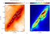 |
Fig. 3 a): Herschel-based Tdust map of TMC-1. The numbers indicate the positions where high S/N NH3(1, 1) and (2, 2) spectra were taken and used to calculate the physical parameters of the gas (see Table 2). b) Herschel-based N(H2) map with the NH3(1, 1) main group integrated intensity contours: 0.6, 1.0, and 2.0 Kkm s-1 (20, 35, and 65% of the maximum). The secondary line components were subtracted from the spectra. Black ellipses indicate the two PGCCs in TMC-1. The positions of TMC-1 CP, TMC-1(NH3), the SO peak, and IRAS 04381+2540 are indicated with a diamond, a triangle, a square, and an asterisk, respectively. HPBW of 40″ is shown in the left bottom corner. |
The N(H2) distribution calculated this way does not exclude the contribution of structures in the foreground or background of HCL 2. In order to correct for this, the extent of HCL 2 was indicated with the AV = 1 magnitude contour (9.4 × 1020 cm-2, where interstellar hydrogen starts to become molecular; Bohlin et al. 1978) on the N(H2) map derived as written above. Then the average 250, 350, and 500 μm intensity at this contour was subtracted from the corresponding SPIRE 250, 350, and 500 μm maps. The final Tdust and N(H2) maps were calculated from these background subtracted intensity images. Other methods of background subtraction are evaluated in Appendix A.1.
Pagani et al. (2015) concluded that a single-temperature SED fitting we use here may miss some of the cold dust in dense cores, thus we probably slightly underestimate the total column density. With only three SPIRE data points, we cannot fit multi-temperature SEDs to model an even colder component but this can be checked with independent methods, such as star-reddening. Malinen et al. (2012) compared FIR emission-based and NIR reddening-based N(H2) values in HCL 2, and they found that the two methods are in good agreement. A significant source of uncertainty in the N(H2) calculation is the error in the surface brightness, as shown by Juvela et al. (2012) using Monte Carlo simulations. Assuming a 13% uncertainty in the Herschel intensities an error of less than 1.5 K appears in regions with temperatures below 16 K. This corresponds to an error in N(H2) of a few times 1021 cm-2 in the outer region of the filament and around 1−2 × 1022 cm-2 in the densest regions.
3. Results
3.1. Tdust and N(H2) distribution from Herschel data
The Herschel-based N(H2) map of HCL 2 is shown in Fig. 1, in which the PGCCs are represented by numbered ellipses. All PGCCs with flux quality of 1 (flux density estimates S/N> 1 in all bands) and 2 (flux density estimates S/N> 1 only in the 857, 545, and 353 GHz Planck bands) are plotted on the figure. Table 1 contains the calculated parameters of these PGCCs, where the columns are: (1) number, also in Fig. 1; (2) PGCC ID; (3, 4) equatorial coordinates; (5, 6) Tdust,min minimum and Tdust,ave average colour temperature in the clump; (7, 8) N(H2)max maximum and N(H2)ave average column density in the clump; and (9) other IDs of the clump. The PGGCs in TMC-1, TMC-1C, and HCL 2B are similarly cold with Tdust,min ≤ 11 K and dense with N(H2)ave ≥ 7 × 1021 cm-2.
The Herschel Tdust map of TMC-1 is shown in Fig. 3a with the positions of high NH3(2, 2) S/N spectra, where temperatures and densities from the NH3 data could be calculated (see Sect. 3.2). Tdust has a minimum of 10.4 K in the northern, densest region and is 11 K at its southern end. The lower density outskirts are a few K warmer.
The Herschel N(H2) map of TMC-1 is shown in Fig. 3b with the NH3(1, 1) main group integrated intensity contours overplotted (the secondary line components were already subtracted from the spectra). Both PGCC G174.20-13.44 and PGCC G174.40-13.45 are indicated by ellipses and the positions of TMC-1 CP, TMC-1(NH3), the SO peak, and IRAS 04381+2540 are also indicated. The map shows TMC-1 as a narrow ridge with an average diameter of 3−4′ (0.12−0.17 pc). Three local N(H2) maxima appear in TMC-1. Two very elongated maxima are located along the ridge with peaks 2′ north-west from TMC-1(NH3) with N(H2) = 3.3 × 1022cm-2 and ≈30″ south-west from TMC-1 CP with N(H2) = 2.7 × 1022cm-2. The third local N(H2) maximum is at ≈18″ south-east from the position of the Class I protostar IRAS 04381+2540 with N(H2) = 2.8 × 1022 cm-2. The PGCCs ellipses coincide with the northern and the southern maxima. The cloud regions cannot be simply separated by the half power contours, since the column density remains above 1022 cm-2 in the central ridge along the filament. We cannot achieve a robust separation of substructures inside TMC-1 (see Appendix C.1) using the N(H2) distribution only.
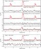 |
Fig. 4 Top: multiple HFS line profile fitting of NH3(1, 1) on the (−400, 520) offset. The spectrum shows one of the brightest secondary line components and gives the lowest Tkin value; see position #4 in Table 2. Box 1: single HFS line profile fit; box 2: residual from the single HFS fit; box 3: simultaneous HFS profile fitting of both components; box 4: the residual from the simultaneous HFS fit; box 5: the residual from the single HFS fit with the HFS fit of the secondary component shown in box 4. Bottom: single NH3(1, 1) HFS line profile fit on position #8 and the residual after subtracting the fit. This position has the highest HFS linewidth from the spectra in Table 2. We note the different scales for the (1, 1) and (2, 2) lines. |
3.2. Results from NH3 measurements
The NH3(1, 1) integrated intensity contours coincide well with the N(H2) distribution, as seen in Fig. 3b. The integrated intensity has a peak at the densest, coldest region of the filament, ≈1′ to the south-east of TMC-1(NH3), and then the line intensities decrease gradually towards the southern edge, while N(H2) remains over 1022 cm-2 even at the southern end of the ridge.
The measured NH3(1, 1) primary component HFS linewidths are in the range of 0.15−1.0 km s-1 with an average of Δv of 0.39 km s-1. As a result of the small linewidths and our high velocity resolution, we were able to separate subregions by their velocities and identify multiple velocity components. The spatial distribution of velocities of the NH3(1, 1) lines with S/N> 3 on 171 positions are plotted in Fig. 5a. The area indicated by these positions is above the Herschel-based 1022 cm-2 column density contour. At the northern region of the ridge the velocities are around 5.9−6.0 km s-1 and most spectra show a secondary line component with velocities around 5.2−5.5 km s-1. South-west of the main ridge, near the Class I young stellar source (Terebey & Baud 1980) IRAS 04381+2540, the primary line velocities are lower (vLSR ≈ 5.2 km s-1). The secondary line components in this same region have vLSR ≈ 5.9 km s-1, except for one component that has 5.6 km s-1. There is a 4.9 km s-1pc-1 velocity gradient seen in the middle section (25:41:00 < δ (2000) < 25:47:00). The primary line component velocities decrease southwards from the mid-region of the ridge from 5.9 to 5.5 km s-1, while the secondary component velocities increase.
The N(NH3(1, 1)) was calculated on 82 positions that are all above the 1.3 × 1022 cm-2Herschel contour; see Fig. 5b. The N(NH3(1, 1)) distribution follows well the Herschel-based N(H2) and reaches 1.5 × 1014 cm-2 even around the CP peak. Its maximum (1.4 × 1015 cm-2) is at the offset of (−320, 440), with absolute coordinates of α(2000) = 04:41:13, δ(2000) = 25:48:47 (position 7 in Fig. 3b). That is ≈1′ to north-west of the position which was formerly known as the ammonia peak, i.e. TMC-1(NH3).
The NH3(2, 2) line was detected with S/N> 3 in as many as 17 spectra, we indicate the corresponding locations in TMC-1 as position #s where the number s runs from 1 to 17 (see Fig. 3a). Parameters at these positions were calculated according to Sect. 2.3 and the results are listed in Table 2. The derived Tkin values vary between 9 and 13 K with the exception of position #10 with 13.7 K. The NH3 column density is 2.8 × 10¹⁴ < Np(NH3) < 1.4 × 1015 cm-2 and the H2 volume density is around 0.4 × 10⁴ < n(H2) < 2.8 × 104 cm-3. The Np(NH3) distribution generally follows the Herschel-based N(H2) distribution along the ridge, although their linear correlation is not very high (the correlation coefficient is p = 0.4). The N(NH3(1, 1)) maximum coincides with the Np(NH3) = Np(NH3)prim + Np(NH3)sec maximum on position #7 and this should be considered as the new NH3 maximum of TMC-1.
Results from our NH3 and the Herschel observations.
We calculated the NH3 relative abundance at our NH3 peak and close to TMC-1 CP using the derived N(H2) and Np(NH3) values in Table 2. This gives 5 × 10⁻⁸ and 1.4 × 10⁻⁸ for the NH3 peak and TMC-1 CP, respectively, which are consistent with the estimates of Harju et al. (1993) for dense cores in Orion and Cepheus (1−5 × 10⁻⁸) and with the chemical modelling of Suzuki et al. (1992) (around 10-8). Generally we find higher abundances in the northern and mid-region of TMC-1 and lower values around the YSO and in the southern end.
The total velocity dispersion was calculated from the primary NH3(1, 1) component of the 17 high S/N spectra with  (10)where Δv is the HFS linewidth. The thermal component of the velocity dispersion is
  (11)where μNH3 = 17 is the ammonia molar mass and mH is the atomic mass unit. The non-thermal (turbulent) component was then derived by
  (12)The thermal component is around 0.066−0.08 km s-1 in the 17 spectra and the non-thermal component is higher than this in almost every case, except on positions #1 and #10. The highest turbulence is observed on positions #8, #13, and #16.
4. Discussion
4.1. Density, temperature, and velocity structure
We obtained the most extensive NH3 map of TMC-1 so far, in which both the (1, 1) and (2, 2) transitions were measured with a low noise level and high velocity resolution. Our observations confirm the variation in the NH3(1, 1) line intensity in TMC-1 that was described by several studies (Little et al. 1979; Olano et al. 1988; Hirahara et al. 1992; Pratap et al. 1997). Our average HFS linewidths agree with the values of Tölle et al. (1981), although we mapped a significantly larger area.
Olano et al. (1988) measured NH3(1, 1) with similar beam size, velocity resolution, and S/N in the high-density region of TMC-1. These authors also observed the velocity difference between the middle section of the ridge and its southern end and a considerably different velocity for the region around IRAS 04381+2540 (see their Fig. 9.). They pointed out a velocity gradient across the ridge as well. We were able to detect further velocity variations because our mapping extends further along and across the ridge compared to theirs.
The Tex values we derived agree well with the 4−7 K range given by Tölle et al. (1981). Their observations do not completely overlap with ours because they measured positions with a spacing of 45″, but the difference between their values and ours on positions of less than 35″ apart is less than 25%, relative to their values. These authors calculated Trot on two positions that are relatively close (≈40″ and ≈5″) to our positions #11 and #15: their values are 9.5 ± 1 K and 10.3 ± 2 K and we derived 8.8 K and 10.5 K, respectively. Gaida et al. (1984) repeated NH3(1, 1) and (2, 2) measurements for the positions of Tölle et al. (1981) along the main ridge of TMC-1 and made two cuts perpendicular to the major axis as well. They calculated both NH3 column densities and kinetic temperatures on three positions that are not farther than 40″ from our position #11, #13, and #15. Their Tkin and Trot results are in agreement with ours, but their N(NH3(1, 1)) values are consistently 4−5 times higher than ours and N(NH3) only agrees well on the higher density positions. Their vLSR and n(H2) distribution along the main ridge also shows similar values to those that we measured. Our Tex values are somewhat lower than those by Olano et al. (1988) (6−9 K), which they show on a plot along the TMC-1 major axis. Their sample does not overlap with our sample either because they used different (0, 0) offset coordinates.
Pratap et al. (1997) and Hirahara et al. (1992) derived a factor of 5−6 higher than our results of H2 volume densities from HC3N and C34S spectra. Our NH3 measurements may not trace the densest gas in TMC-1 because, as shown by Bergin et al. (2002) and Pagani et al. (2005), NH3 is best used as a tracer at lower than 5 × 105 cm-3 densities. Also, because of the low critical density (around 2 × 103 cm-3) of the (1, 1) line, it may have a substantial contribution from external, warmer layers as well (Pagani et al. 2007). Our results do not show significant differences in volume densities along the ridge, while the observations by Hirahara et al. (1992) imply a gradient of a factor of 10 in n(H2) between TMC-1(NH3) and TMC-1 CP. The NH3 densities calculated by Tölle et al. (1981) at TMC-1(NH3) are consistent with our results, but their values are a factor of 2−3 higher at TMC-1CP. The results by Pratap et al. (1997) are consistent with our results at TMC-1 CP but a factor of 2−3 lower than our values in the northern region.
Nutter et al. (2008) presented temperature and density profile modelling for TMC-1 based on SCUBA, IRAS, and Spitzer continuum data. Their best fit was given by an inner colder filament (8 K) and an outer layer (12 K) and resulted in n(H2) values in the range of 0.7−1.75 × 105 cm-3. They also calculated N(H2) from the 850 μm SCUBA map, which yielded 3.8 × 10²² and 4.4 × 1021 cm-2 for the central region and the outer layer, respectively. Malinen et al. (2012) used 2MASS and Herschel maps to derive the properties for TMC-1. Their results are consistent with the findings of Nutter et al. (2008) and their N(H2) peak is around 3.4 × 1022 cm-2. This is our derived N(H2) maximum as well. We note that our calculations are based on point source subtracted Herschel images. The Tdust values that we derived for the outer region of TMC-1 are consistent with the 12 K from Nutter et al. (2008), but we measure 10 K in the inner region instead of 8 K. The Tkin derived from NH3 and Tdust derived from the Herschel measurements vary similarly but do not agree well, since the cooling-heating processes are different for gas and dust and the coupling of the two phases are not guaranteed in regions with n(H2) = 104 cm-3 (Goldsmith 2001).
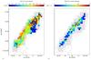 |
Fig. 5 a): vLSR distribution of the main (or only) line component of the NH3(1, 1) lines with S/N> 3. Circles indicate the positions where a secondary component was found and their color corresponds to the velocity of this component. b): N(NH3(1, 1)) distribution map calculated on positions where the τ optical depth from single HFS profile fit had an error of less than 50%. The grey area shows the total extension of the observed NH3 map and the grey contours are the Herschel N(H2): 0.7, 1.0, 1.3, 1.6, 2, 2.3, 2.6 × 1022 cm-2 (from 20 to 80% of the maximum by 10%). The positions of TMC-1 CP, TMC-1(NH3), the SO peak, and IRAS 04381+2540 are indicated as before and the position of our NH3 peak is indicated with an upside down triangle. |
4.2. Substructures in TMC-1
4.2.1. Clustering methods and their results
The complex velocity structure and the appearance of secondary velocity components on several spectra suggest that different cloud parts are present in TMC-1. Since the filament is not necessarily one coherent structure and it could be interpreted as a chain of clumps, or even a complex superposition of filaments containing smaller scale cores, we apply several types of clustering methods to reveal its morphology.
Clump-finding in the NH3 PPV datacube with methods like the 3D version of clumpfind, gaussclump, or the dendogram technique (see Appendix C.1) is problematic in the case of TMC-1, since NH3 abundance can be position-dependent in the cloud. Moreover, NH3 alone is not a good tracer for clumps because of high optical depth effects such as self-absorption, which affects the line profiles. Searching for clumps in the Herschel-based N(H2) distribution is not enough either, since N(H2) changes smoothly along the ridge. As we can see from a quick decomposition of the filament with clumpfind in Appendix C.1, we do not get a robust result; the extent and shape of the derived clumps strongly depend on the initial parameters given to the clump finding algorithm. Also, this way we ignore the velocity information derived from molecular emission that traces the relative motions of the gas and can help identify structures in the line of sight.
We expect that the presence of a clump changes the N(H2) distribution in its direction. We assume that inside a clump N(H2) changes continuously, velocities scatter around a certain value and the clump appears as an object roughly in the same direction on the plane of the sky. Thus, we combine the vLSR derived from the HFS line profile fit of the NH3(1, 1) primary components and the Herschel-based N(H2) values on every position where the (1, 1) line was observed with S/N> 3. Then we search for clusters in this datacube consisting of position, position, velocity, and column density. The importance of the secondary line components is discussed later (see Sect. 4.2.2).
The number of clusters in the cloud was not known and we did not want to decide which clustering method to use for the proportioning beforehand. Because of this we used the NbClust algorithm of the R statistical computing environment (Charrad et al. 2014), which is able to run several types of clustering methods while varying the number of clusters to be derived. It computes so-called cluster validity indices to inspect the results of the different runs, decides what is the most appropriate number of clusters in a dataset, and also performs the clustering itself. The NbClust algorithm is able to run the k-means method (see Appendix C.2) and hierarchical agglomerative clustering (HAC) methods with eight different agglomeration criteria (see Appendix C.3). A more detailed description of the NbClust package and the indices used can be found in Appendix C.4.
Since our parameters in the dataset are measured on different scales, standardization is necessary. We converted the position offsets to galactic offsets in arcminutes, velocity to tenth of km s-1 and column density to 1021 cm-2 to bring the parameter ranges closer to each other. Then we used the min-max scaling where the normalized value of parameter pi of the nth point in the dataset is defined by  (13)where pi are the four parameters (Δl, Δb, vLSR, N(H2)) of an x = [p1, p2, p3, p4] point in the 4D parameter space with n points. The min-max scaling or scaling by the range of the variables was shown to give more accurate results for the most known clustering techniques than results found with traditional standardization methods, such as z-score (Steinley 2004).
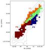 |
Fig. 6 Resulting clusters from the k-means clustering method projected back to the plane of the sky. The grey contours are the Herschel N(H2): 0.7, 1.0, 1.3, 1.6, 2, 2.3, 2.6 × 1022 cm-2 (from 20 to 80% of the maximum by 10%). The positions of TMC-1 CP, IRAS 04381+2540, the SO peak, and our NH3 maximum are indicated as before. |
The NbClust algorithm also requires the definition of a distance metric. We used Euclidean distance metric where the distance between two points (x1 and x2) in the i = 4 dimensional parameter space is  (14)We can then define within-cluster and between-cluster distances for points inside one cluster and of two different clusters, respectively.
The nine available clustering methods in NbClust were run on the scaled and normalized TMC-1 joined dataset. When determining the ideal number of clusters with a certain clustering method, the number of clusters that was allowed to be derived varied from 2 to 15. The NbClust algorithm computed 30 indices to measure the validity of the derived clusters (see Appendix C.4) in each case. Each index suggested the ideal number of clusters that should be derived by the method and the final decision was made by the majority rule. After this the clustering was performed. The final results of the nine clustering methods are plotted on Fig. C.2.
Four clustering methods provided similar division of TMC-1 into four parts; see Figs. C.2b, c, d and 6. The HAC method with the average agglomeration criterion derived three clusters (Fig. C.2e), McQuitty’s criterion derived 15 parts (Fig. C.2a), and the HAC method with the median, centroid and single agglomeration criteria did not part the filament (Fig. C.2f−h).
In order to decide between the results of the nine clustering methods, the sum and the weighted sum of the within-cluster variances were determined for each method. We first calculated the variance of the distances of all cluster members from the cluster centres in every cluster resulted by each clustering method with 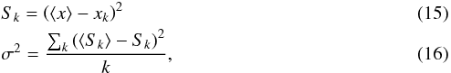 where k is the index of points inside a cluster, Sk are the distances of each cluster member (xk) from the cluster centre (⟨ x ⟩) in each cluster, and σ2 is the variance of these distances for each cluster. Then we calculated a sum (Cm) and a weighted sum (Cm,w), adding together the cluster variances of the clusters belonging to each clustering method with
 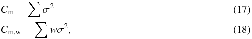 where w weight is the number of pixels in a cluster. The most appropriate number of clusters and the number of indices suggesting that number are found in Table 3 for each clustering method, along with the derived sum and weighted sum of variances for the methods.
Results from the NbClust method.
The HAC method with McQuitty’s agglomeration criterion derived the clusters with the minimal sum and weighted sum of variances in the 4D-parameter space. However, when the clusters are projected back to the sky we find one fragment that is too small (only 3 pixels), and three fragments that are not continuous, but each of these fragments is broken into two or three isolated parts. The existence of several very small fragments may be proved measuring several chemical species and using high spatial resolution and small spacing, but in the current study we accept the results of the k-means method as best, which had the second minimal sum of within-cluster variances.
The four clusters resulted by the k-means method were projected back to the plane of the sky, defining four objects, each of which is contiguous (see Fig. 6). Three of these sub-filaments are very elongated (TMC-1F1, TMC-1F2, TMC-1F4) and one of them (TMC-1F3) is less so. TMC-1F1 appears with the highest velocities and column densities, while TMC-1F2 on the north-eastern edge has the lowest kinetic temperature. The environment of the YSO makes up TMC-1F3. TMC-1F4 encompasses the middle and southern regions with a range of velocities and has the highest average linewidth.
The secondary NH3(1, 1) line components in TMC-1F3 appear at a velocity of the neighbouring TMC-1F1. Similarly, the secondary NH3(1, 1) line components in TMC-1F1 appear at 5.2−5.4 km s-1, i.e. the velocity of TMC-1F3. The kinematics thus suggests that the clumps are slightly overlapped. Few spectra with secondary components in TMC-1F4 indicate small fragments with velocities similar to that of TMC-1F1 and TMC-1F2.
Despite the scaling and normalization of the parameters of the joined dataset, the Euclidean distance measured in one dimension cannot be unequivocally compared with the distance measured in another, since the parameters are independent and not interchangeable. For example, the min-max normalization only works well if the dispersion in each dimension is small and there are no extreme points that distort the calculations. The careful selection of the 82 spectral positions with high S/N NH3 measurements and smoothly changing N(H2) ensures that this is not the case in this dataset. However, to reveal the discrepancies originating from using these statistical methods with a dataset like this, in a later study our methods should be carried out side by side with other clump-finding methods on a more extended dataset, where the decomposition of the molecular cloud is known, can be verified, and the results can be compared.
4.2.2. The parameters and stability of the sub-filaments
Averaged Herschel-based Tdust,ave were calculated inside the sub-filament contours and were found to be the same within 0.5 K for each sub-filament. The Tkin,ave kinetic temperatures of the sub-filaments were calculated as an average of the corresponding Tkin values on the positions of the 17 high S/N NH3(2, 2) spectra (see Table 2) inside the given sub-filament. Apparently, Tkin shows a higher variation than Tdust, which is also seen in the averaged values. Background corrected column densities were calculated for each sub-filament subtracting an average background N(H2) of HCL 2. Then the total hydrogen mass was calculated integrating inside the sub-filament boundary. In our simplified assumptions the sub-filaments are considered cylinders with L length and r radius and they are roughly perpendicular to the line of sight. Their maximum diameter along the galactic plane is L and r is half of their diameter perpendicular to this. The linear mass of the sub-filaments was calculated dividing their mass with the L length. TMC-1F1 has the highest N(H2)ave value and TMC-F4 has the highest mass.
The greatest uncertainty of the mass calculation is the error in the N(H2) distribution caused by the ≈1.5 K uncertainty of the Tdust map. According to this, the calculated linear masses can have an error up to 56%. We note here that the uncertainty of the Tdust values was a conservative estimate but still this error makes our virial stability consideration uncertain. Additionally, because our sub-filaments overlap, N(H2) derived from the dust emission originates from more than one structure. The ratio of Np(NH3) derived from the secondary components and the total Np(NH3) is around 10%. If we assume that the relative abundance of NH3 does not change much inside a sub-filament, this means that the ratio of Np(NH3) from the main and secondary line components reflects the ratio of N(H2) between the two overlapping cloud parts. Thus we can say that the contribution of the overlapping part of a sub-filament to the mass of the other one is negligible.
We calculated the total (σtotal,ave), the thermal (σth,ave) and non-thermal velocity dispersion (σnth,ave) inside each sub-filament from the Δv HFS linewidth of their averaged spectra with Eqs. (10)−(12). We note that the total velocity dispersion includes the velocity gradients inside the sub-filaments; these are 0.18, 0.15, 0.03, and 0.35 km s-1 pc-1 for TMC-1F1 to F4, respectively. Then the virial mass per unit length of the sub-filaments could be derived with 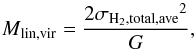 (19)where σH2,total,ave is the total velocity dispersion of the hydrogen (Ostriker 1964). This is calculated as
 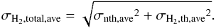 (20)The physical parameters of the sub-filaments are listed in Table 4. The mass of the sub-filaments are slightly above (TMC-1F1 and TMC-1F4) or below (TMC-1F2 and TMC-1F3) their virial mass per unit length but with uncertainties around 50% in the observed linear masses we can only safely say that all of them are close to equilibrium. The non-thermal support of the sub-filaments is generally 2−2.5 times higher than the thermal. We note that there is no significant difference between the parameters of the clusters (size, shape, masses) from the k-means and the other clustering methods that also derived four clusters.
4.2.3. Sub-filaments TMC-1F1, TMC-1F2, and TMC-1F4
Our results show that the main ridge of TMC-1 can be resolved into three sub-filaments. A minimal overlap of TMC-1F4 and TMC-1F2 or the presence of other small fragments is seen in the middle of the ridge in the presence of secondary line components. Otherwise these sub-filaments are very well separated. TMC-1F4 has the highest average turbulent velocity dispersion. The N(NH3(1, 1)) distribution peaks inside TMC-1F1 (see the upside down triangle in Fig. 5b), which is also the position of the maxima of Np(NH3) and n(H2) (see Table 2).
Snell et al. (1982) observed TMC-1 in C34S(1−0) and (2−1) and divided it into six fragments ([SLF82] A to F), many of which were overlapping. The position, extent, and velocity of [SLF82] B and [SLF82] C roughly correspond to TMC-1F4. Their [SLF82] A, [SLF82] D, and [SLF82] F coincide with the positions of TMC-1F1 and TMC-1F2, and the velocities of [SLF82] D and [SLF82] F are also similar to that of TMC-1F1 and TMC-1F2.
Hirahara et al. (1992) found six cores on CCS emission maps of TMC-1. In the northern region, their core A and B (TMC-1B) coincide with the northern region of our TMC-1F1 and the overlapping section of TMC-1F3, which we detected with the secondary line components. They divide our TMC-1F4 into two parts, namely core C and D (TMC-1D) based on their CCS channel maps. We note however that they appear as one object with some structure on their CCS position-velocity and HC3N integrated intesity maps. Their core E (TMC-1E) is positioned south-east of the southern edge of TMC-1F4, where we did not detect significant NH3(1, 1) emission. Associations of the sub-filaments and these formally known parts of TMC-1 are in Table 5.
Our sub-filaments and the coinciding objects.
Pratap et al. (1997) mapped TMC-1 in SO(32−21), CS(2−1), and HC3N(4−3) and (10−9). Their SO peak is ≈1′ north-east from our NH3 peak in TMC-1F2, which we also recognize in their SO channel maps. TMC-1F4 appears as an elongated maximum of the HC3N(4−3) and (10−9) integrated intensity (see Fig. 7. in Pratap et al. 1997). A secondary maximum is seen in HC3N integrated intensity maps inside our TMC-1F1. The relative density maxima of sulfur and nitrogen-bearing molecules are in the northern sub-filaments, whereas TMC-1F4 is the relative density maximum region of the carbon-chain molecules. The cyanopolyyne peak TMC-1 CP is roughly in the middle of TMC-1F4.
TMC-1F1 and TMC-1F4 are associated with two and one 350 μm Herschel point sources, respectively. We cannot exclude that the higher Tkin measured at position #1 (see Table 2) is related to the nearby Herschel point source, although we do not measure an increased temperature at position #2. The nature of the Herschel FIR point sources, other NIR point sources in the region (see e.g. Tóth et al. 2004) and their relation to the ISM will be discussed in future work.
We note that the HAC method with McQuitty’s agglomeration criterion defines 12 sub-filaments in the main ridge (M1 to M12 in Fig. C.2a). None of those have the same position, velocity, and extent as any of the Snell et al. (1982) or Hirahara et al. (1992) fragments, but the fragment M4 that coincides with the Np(NH3) and N(H2) peak region, is located close to fragment A by Hirahara et al. (1992), although it has a greater extent.
4.2.4. Sub-filament TMC-1F3 and the Class I protostar IRAS 04381+2540
TMC-1F3 is separated from the main filament both in position and velocity. The velocity and position of a CS local maximum, Snell et al. (1982) fragment A, roughly corresponds to TMC-1F3. Their Fig. 8 also indicates that TMC-1F3 partly overlaps with the main ridge. The displacement of the CS peak may be partly due to their low resolution (HPBW ≈ 2′) or a chemistry effect. TMC-1F3 corresponds to TMC-1X (identified as core X in the CCS(4−3) position-velocity maps) of Hirahara et al. (1992). TMC-1F3 also appears at similar velocities but with different extent in their HC3N(5−4) integrated intensity and NH3(1, 1) channel maps. The overlap with the main ridge is also apparent in their figures. One may recognize TMC-1F3 in the CS and SO integrated intensity maps of Pratap et al. (1997).
TMC-1F3 was also located by Yıldız et al. (2015) in 12CO with a velocity of 5.2 km s-1. The position of TMC-1F3 coincides with that of the protostar IRAS 04381+2540 (Beichman et al. 1986) that is known to drive a bipolar outflow detected in 12CO (Bontemps et al. 1996) and H2 (Gomez et al. 1997). Its disk was resolved and a YSO mass of 0.54 M⊙ was estimated by Harsono et al. (2014). Apai et al. (2005) described it as a binary in formation with a jet and substellar companion and showed that the northern outflow cavity is opening towards us. According to Yıldız et al. (2013), the velocity of the YSO is vLSR = 5.2 km s-1, which agrees with that of our NH3 clump (5.2−5.4 km s-1). The non-thermal velocity dispersion of TMC-1F3 is the second highest and its thermal velocity dispersion is the highest of all four sub-filaments.
From the positional coincidence and velocity one may assume that the Class I protostar is related to the sub-filament. The relatively high average kinetic temperature (13 K, see Table 4) of TMC-1F3 we interpret as a possible signature of the heating by IRAS 04381+2540. In fact the highest kinetic and dust temperatures were measured at the YSO position (see position #10 with Tkin ≈ 14 K and Tdust = 11.4 K in Table 2).
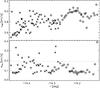 |
Fig. 7 Central velocity and non-thermal velocity dispersion of the NH3(1, 1) primary components along TMC-1F4 (crosses) and TMC-1F1 (circles) from left to right. The sound speed in the two clumps are indicated with a dashed line in the lower panel. |
The highest HFS linewidth of the NH3(1, 1) primary line components is at position #8 and around it (Δv = 0.39 km s-1, Tkin = 10.6 K, see Table 2) in TMC-1F1. The appearance of increased linewidths could be explained by the outflow of IRAS 04381+2540 (120″ south-west of #8) releasing mechanical energy towards the main ridge. The outflow is very compact, however, with a lobe extent of only around 40″ to the north and south according to Hogerheijde et al. (1998) and Yıldız et al. (2015). The northern outflow lobe is blue-shifted, opening towards the observer, thus the protostar has to be positioned behind the main ridge and the outflow should extend to at least 120″ (projected distance of position #8) to affect the main ridge. Hogerheijde et al. (1998) calculated a dynamical age of 2100 yr from a 12CO(3−2) outflow extent of 0.02 pc and outflow velocity of 9.3 km s-1. One may however assume that a jet with about an order of magnitude higher speed propagated to more than 0.1 pc in the same time interval. We note here that velocities up to 70 km s-1 were also observed at very low-mass YSOs (see e.g. ISO 143 in Joergens et al. 2012). Our assumption from the above geometry is that the protostar IRAS 04381+2540 is embedded in TMC-1F3, which may be located around 0.1 pc behind the main ridge.
4.2.5. Fray and fragment?
The primary NH3(1, 1) line component vLSR velocity distribution in TMC-1F1 and TMC-1F4 is continuous, as seen in Fig. 7. A velocity gradient of ≈0.45 km s-1pc-1 is seen from SE to NW. An oscillating behaviour can be observed above the gradient in both sub-filaments, but with a higher dispersion in TMC-1F4, and the wavelength of the periodical change in TMC-1F1 from a sinusoidal approximation is ≈0.3 pc. Similar velocity oscillations were observed in several filaments in L1517 (Hacar & Tafalla 2011) together with sinusoidal column density oscillations as evidence of core formation. The non-thermal velocity dispersions also show oscillations and are mostly subsonic, since the typical sound speed,  km s-1 in the two sub-filaments. Supersonic points could be explained by confusion of multiple velocity components or outflows from embedded sources inside the sub-filaments. The pattern of velocity dispersions may indicate that the sub-filaments are decoupled from the large-scale turbulent velocity field and the turbulent dissipation in the cloud occurred at the scale of the sub-filaments (Tafalla & Hacar 2015).
Comparing the position-velocity diagram of TMC-1F1 and TMC-1F4, the latter looks less regular. Analysing a dust continuum map of TMC-1, Suutarinen et al. (2011) suggested that the southern half of the ridge has an extensive envelope, in contrast to the northern, i.e. the NH3 peak region. They explain this as a difference in dynamical age: the northern region is more compressed. Based on time dependent modelling of the observed variation of chemistry they also concluded that the south-eastern end of the cloud is also chemically less evolved than the north-eastern end. The difference in the chemical ages of TMC-1F1 and TMC-1F4 was also indicated by Berczik et al. (2015).
Peng et al. (1998) studied the fragmentation in a 8′ × 8′ region around TMC-1 CP in TMC-1F4 with CCS measurements. They found 45 very small fragments with sizes of 0.02−0.04 pc and masses of 0.04−0.6 M⊙; five of those fragments were gravitationally bound. The northern end of TMC-1F4 was resolved into cores with sizes of 0.03−0.06 pc and masses of 0.03−2 M⊙ by Langer et al. (1995), based on high resolution single-dish and interferometric observations of CCS and CS.
Hierarchical fragmentation was found by Hacar et al. (2013) and Tafalla & Hacar (2015) in the nearby L1495/B2013 complex. The fray and fragment filament evolution scenario proposed by these authors is the following: The filamentary cloud first fragments into intertwined, velocity-coherent filaments, so-called fibers. If the fiber can accumulate enough mass to become gravitationally unstable, it can further fragment into chains of closely spaced cores in an almost quasi-static way. As seen in Table 4, the length of TMC-1F1, TMC-1F2, and TMC-1F4 is similar that of the fibers in L1495/B2013. The typical length of the fibers of Hacar et al. (2013) is 0.5 pc (ranging from 0.2 pc to 1.2 pc). TMC-1F2 even has a similar linear mass as the fiber [HTK2013] 32 of Hacar et al. (2013). However their typical 0.5 pc-long fibers have a factor of two lower mass than the sub-filaments of TMC-1. Some of their fibers are unstable and fragmented into chains of cores.
The velocity and linewidth distributions in TMC-1F1 in the northern region of TMC-1 is very similar to that of the fibers described by Tafalla & Hacar (2015). The southern section of TMC-1 with TMC-1F4 is said to be structurally and chemically less evolved than the northern region of TMC-1, also the velocity dispersion is much higher in TMC-1F4 than in TMC-1F1. However, there are already small, gravitationally bound cores inside TMC-1F4. It is not clear whether fray and fragment is the process shaping TMC-1 because we cannot simply say that the filament first collapsed into velocity-coherent fibers and then formed cores inside them. One has to see the distribution of small-scale structures all along TMC-1 and discuss again the fray and fragment scheme.
5. Conclusions
Our work contributes to the study of HCL 2, focussing on the TMC-1 region based on Herschel SPIRE FIR and high S/N NH3 1.3 cm line mapping. We found TMC-1 as one of the coldest and densest regions of HCL 2 (along with TMC-1C and HCL 2B) from our N(H2) and Tdust calculations.
Our Herschel-based N(H2) shows values above 1022 cm-2 with two local maxima along a narrow ridge. The northern maximum is the peak N(H2) position with 3.3 × 1022 cm-2. There is a third, more separated peak south-west from this. Tdust is almost constant along the higher density inner region of the ridge.
Fitting multiple HFS line profiles to the NH3(1, 1) spectra we identified multiple velocity components in the northern region and calculated low turbulent velocity dispersions (0.1−0.2 km s-1). The derived N(NH3(1, 1)) distribution follows the Herschel-based N(H2) distribution well. We define a new NH3-peak in an offset of ≈1′ relative from TMC-1(NH3). The NH3-based n(H2) are lower than former C34S and HC3N-based values by a factor of 5−6.
Based on the observed velocity and column density variations we partitioned TMC-1 using the NbClust package of R. The four derived sub-filaments have masses of 20−40 M⊙, three of these sub-filaments are very elongated (TMC-1F1, TMC-1F2, TMC-1F4) and all of them close to gravitational equilibrium. TMC-1F1 has the NH3 peak and TMC-1F4 the cyanopolyyne peak inside. TMC-1F3 partly overlaps with TMC-1F1, and the Class I protostar IRAS 04381+2540 is apparently embedded into this sub-filament. The protostellar outflow is probably affecting TMC-1F1. The fray and fragment process is one possible scenario for the structuring of TMC-1, but the small-scale structure of TMC-1F1 should be investigated to ascertain this scenario.
A more detailed description and analysis could be given with a high resolution survey of the whole TMC-1 in carbonous and nitrogen bearing molecules (e.g. CCS and NH3 lines) and, subsequently, using chemical and radiative transfer models in the interpretation.
Herschel interactive processing environment, http://herschel.esac.esa.int/hipe/
Acknowledgments
This research was partly supported by the OTKA grants K101393 and NN-111016 and it was supported by the Momentum grant of the MTA CSFK Lendület Disk Research Group. The research leading to these results has received funding from the European Commission Seventh Framework Programme (FP/2007-2013) under grant agreement No 283393 (RadioNet3). V.-M.P. acknowledges the support of Academy of Finland grant 250741. Valuable discussions with Jorma Harju, Malcolm Walmsley, and Dimitris Stamatellos are acknowledged. We thank the anonymous referee for the careful reading of our manuscript and the valuable comments and suggestions. Herschel was an ESA space observatory with science instruments provided by European-led Principal Investigator consortia and with participation from NASA. SPIRE was developed by a consortium of institutes led by Cardiff Univ. (UK) and including Univ. Lethbridge (Canada); NAOC (China); CEA, LAM (France); IFSI, Univ. Padua (Italy); IAC (Spain); Stockholm Observatory (Sweden); Imperial College London, RAL, UCL-MSSL, UKATC, Univ. Sussex (UK); Caltech, JPL, NHSC, Univ. Colorado (USA). This development was supported by national funding agencies: CSA (Canada); NAOC (China); CEA, CNES, CNRS (France); ASI (Italy); MCINN (Spain); SNSB (Sweden); STFC (UK); and NASA (USA). PACS was developed by a consortium of institutes led by MPE (Germany) and including UVIE (Austria); KUL, CSL, IMEC (Belgium); CEA, OAMP (France); MPIA (Germany); IFSI, OAP/AOT, OAA/CAISMI, LENS, SISSA (Italy); IAC (Spain). This development has been supported by the funding agencies BMVIT (Austria), ESA-PRODEX (Belgium), CEA/CNES (France), DLR (Germany), ASI (Italy), and CICT/MCT (Spain). Based on observations with the 100-m telescope of the MPIfR (Max-Planck-Institut für Radioastronomie) at Effelsberg, the authors thank their high level of technical support and assistance.
References
- André, P., Men’shchikov, A.,Bontemps, S., et al. 2010, A&A, 518, L102 [NASA ADS] [CrossRef] [EDP Sciences] [Google Scholar]
- Apai, D., Tóth, L. V., Henning, T., et al. 2005, A&A, 433, L33 [NASA ADS] [CrossRef] [EDP Sciences] [Google Scholar]
- Bally, J., Langer, W. D., Stark, A. A., & Wilson, R. W. 1987, ApJ, 312, L45 [NASA ADS] [CrossRef] [Google Scholar]
- Beckwith, S. V. W., Sargent, A. I., Chini, R. S., & Guesten, R. 1990, AJ, 99, 924 [NASA ADS] [CrossRef] [Google Scholar]
- Beichman, C. A., Myers, P. C., Emerson, J. P., et al. 1986, ApJ, 307, 337 [NASA ADS] [CrossRef] [Google Scholar]
- Berczik, P., Bertsyk, P., Toth, V., & Baranyai, A. 2015, IAU General Assembly, Meeting 29, 2252605 [Google Scholar]
- Bergin, E. A., Alves, J., Huard, T., & Lada, C. J. 2002, ApJ, 570, L101 [NASA ADS] [CrossRef] [Google Scholar]
- Bohlin, R. C., Savage, B. D., & Drake, J. F. 1978, ApJ, 224, 132 [NASA ADS] [CrossRef] [Google Scholar]
- Bontemps, S., Andre, P., Terebey, S., & Cabrit, S. 1996, A&A, 311, 858 [NASA ADS] [Google Scholar]
- Cambrésy, L. 1999, A&A, 345, 965 [NASA ADS] [Google Scholar]
- Cernicharo, J., & Guelin, M. 1987, A&A, 176, 299 [NASA ADS] [Google Scholar]
- Charrad, M., Ghazzali, N., Boiteau, V., & Niknafs, A. 2014, J. Statistical Software, 61, 1 [Google Scholar]
- Danby, G., Flower, D. R., Valiron, P., Schilke, P., & Walmsley, C. M. 1988, MNRAS, 235, 229 [NASA ADS] [CrossRef] [Google Scholar]
- Dobashi, K., Uehara, H., Kandori, R., et al. 2005, PASJ, 57, 1 [Google Scholar]
- Dunn, J. C. 1974, J. Cybernetics, 4, 95 [CrossRef] [Google Scholar]
- Elias, J. H. 1978, ApJ, 224, 857 [NASA ADS] [CrossRef] [Google Scholar]
- Gaida, M., Ungerechts, H., & Winnewisser, G. 1984, A&A, 137, 17 [NASA ADS] [Google Scholar]
- Goldsmith, P. F. 2001, ApJ, 557, 736 [NASA ADS] [CrossRef] [MathSciNet] [Google Scholar]
- Goldsmith, P. F., Heyer, M., Narayanan, G., et al. 2008, ApJ, 680, 428 [NASA ADS] [CrossRef] [Google Scholar]
- Gomez, M., Whitney, B. A., & Kenyon, S. J. 1997, AJ, 114, 1138 [NASA ADS] [CrossRef] [Google Scholar]
- Gower, J. C. 1966, Biometrics, 23, 123 [Google Scholar]
- Griffin, M. J., Abergel, A., Abreu, A., et al. 2010, A&A, 518, L3 [Google Scholar]
- Hacar, A., & Tafalla, M. 2011, A&A, 533, A34 [NASA ADS] [CrossRef] [EDP Sciences] [Google Scholar]
- Hacar, A., Tafalla, M., Kauffmann, J., & Kovács, A. 2013, A&A, 554, A55 [NASA ADS] [CrossRef] [EDP Sciences] [Google Scholar]
- Halkidi, M., Vazirgiannis, M., & Batistakis, Y. 2000, in Principles of Data Mining and Knowledge Discovery, eds. D. Zighed, J. Komorowski, & J. Zytkow (Berlin, Heidelberg: Springer), Lect. Not. Comput. Sci., 1910, 265 [Google Scholar]
- Harju, J., Walmsley, C. M., & Wouterloot, J. G. A. 1993, A&AS, 98, 51 [NASA ADS] [Google Scholar]
- Harsono, D., Jørgensen, J. K., van Dishoeck, E. F., et al. 2014, A&A, 562, A77 [NASA ADS] [CrossRef] [EDP Sciences] [Google Scholar]
- Hatchell, J., Richer, J. S., Fuller, G. A., et al. 2005, A&A, 440, 151 [NASA ADS] [CrossRef] [EDP Sciences] [Google Scholar]
- Heiles, C. E. 1968, ApJ, 151, 919 [NASA ADS] [CrossRef] [Google Scholar]
- Hirahara, Y., Suzuki, H., Yamamoto, S., et al. 1992, ApJ, 394, 539 [NASA ADS] [CrossRef] [Google Scholar]
- Ho, P. T. P., & Townes, C. H. 1983, ARA&A, 21, 239 [NASA ADS] [CrossRef] [Google Scholar]
- Hogerheijde, M. R., van Dishoeck, E. F., Blake, G. A., & van Langevelde, H. J. 1998, ApJ, 502, 315 [NASA ADS] [CrossRef] [PubMed] [Google Scholar]
- Jain, A. K., Murty, M. N., & Flynn, P. J. 1999, ACM Comput. Surv., 31, 264 [CrossRef] [Google Scholar]
- Joergens, V., Kopytova, T., & Pohl, A. 2012, A&A, 548, A124 [NASA ADS] [CrossRef] [EDP Sciences] [Google Scholar]
- Juvela, M., Ristorcelli, I., Pagani, L., et al. 2012, A&A, 541, A12 [NASA ADS] [CrossRef] [EDP Sciences] [Google Scholar]
- Juvela, M., Demyk, K., Doi, Y., et al. 2015a, A&A, 584, A94 [NASA ADS] [CrossRef] [EDP Sciences] [Google Scholar]
- Juvela, M., Ristorcelli, I., Marshall, D. J., et al. 2015b, A&A, 584, A93 [NASA ADS] [CrossRef] [EDP Sciences] [Google Scholar]
- Kirk, J. M., Ward-Thompson, D., Palmeirim, P., et al. 2013, MNRAS, 432, 1424 [NASA ADS] [CrossRef] [Google Scholar]
- Kramer, C., Stutzki, J., Rohrig, R., & Corneliussen, U. 1998, A&A, 329, 249 [NASA ADS] [Google Scholar]
- Langer, W. D., Velusamy, T., Kuiper, T. B. H., et al. 1995, ApJ, 453, 293 [NASA ADS] [CrossRef] [Google Scholar]
- Little, L. T., MacDonald, G. H., Riley, P. W., & Matheson, D. N. 1979, MNRAS, 189, 539 [NASA ADS] [CrossRef] [Google Scholar]
- MacQueen, J. 1967, in Proc. Fifth Berkeley Symposium on Mathematical Statistics and Probability, Vol. 1: Statistics (Berkeley, Calif.: University of California Press), 281 [Google Scholar]
- Malinen, J., Juvela, M., Rawlings, M. G., et al. 2012, A&A, 544, A50 [NASA ADS] [CrossRef] [EDP Sciences] [Google Scholar]
- McElroy, D., Walsh, C., Markwick, A. J., et al. 2013, A&A, 550, A36 [NASA ADS] [CrossRef] [EDP Sciences] [Google Scholar]
- McQuitty, L. L. 1966, Educational and Psychological Measurement, 26, 825 [CrossRef] [Google Scholar]
- Milligan, G., & Cooper, M. 1985, Psychometrika, 50, 159 [CrossRef] [Google Scholar]
- Mizuno, A., Onishi, T., Yonekura, Y., et al. 1995, ApJ, 445, L161 [NASA ADS] [CrossRef] [Google Scholar]
- Murtagh, F., & Heck, A. 1987, Multivariate Data Analysis, Astrophys. Space Sci. Libr., 131 [Google Scholar]
- Murtagh, F., & Legendre, P. 2014, J. Classification, 31, 274 [Google Scholar]
- Myers, P. C., Linke, R. A., & Benson, P. J. 1983, ApJ, 264, 517 [NASA ADS] [CrossRef] [Google Scholar]
- Narayanan, G., Heyer, M. H., Brunt, C., et al. 2008, ApJS, 177, 341 [NASA ADS] [CrossRef] [Google Scholar]
- Nutter, D., Kirk, J. M., Stamatellos, D., & Ward-Thompson, D. 2008, MNRAS, 384, 755 [NASA ADS] [CrossRef] [Google Scholar]
- Olano, C. A., Walmsley, C. M., & Wilson, T. L. 1988, A&A, 196, 194 [NASA ADS] [Google Scholar]
- Onishi, T., Mizuno, A., Kawamura, A., Ogawa, H., & Fukui, Y. 1996, ApJ, 465, 815 [NASA ADS] [CrossRef] [Google Scholar]
- Onishi, T., Mizuno, A., Kawamura, A., Tachihara, K., & Fukui, Y. 2002, ApJ, 575, 950 [NASA ADS] [CrossRef] [Google Scholar]
- Ostriker, J. 1964, ApJ, 140, 1056 [NASA ADS] [CrossRef] [MathSciNet] [Google Scholar]
- Padoan, P., Cambrésy, L., & Langer, W. 2002, ApJ, 580, L57 [NASA ADS] [CrossRef] [Google Scholar]
- Pagani, L., Pardo, J.-R., Apponi, A. J., Bacmann, A., & Cabrit, S. 2005, A&A, 429, 181 [NASA ADS] [CrossRef] [EDP Sciences] [Google Scholar]
- Pagani, L., Bacmann, A., Cabrit, S., & Vastel, C. 2007, A&A, 467, 179 [NASA ADS] [CrossRef] [EDP Sciences] [Google Scholar]
- Pagani, L., Lefèvre, C., Juvela, M., Pelkonen, V.-M., & Schuller, F. 2015, A&A, 574, L5 [NASA ADS] [CrossRef] [EDP Sciences] [Google Scholar]
- Peng, R., Langer, W. D., Velusamy, T., Kuiper, T. B. H., & Levin, S. 1998, ApJ, 497, 842 [NASA ADS] [CrossRef] [Google Scholar]
- Pilbratt, G. L., Riedinger, J. R., Passvogel, T., et al. 2010, A&A, 518, L1 [CrossRef] [EDP Sciences] [Google Scholar]
- Planck Collaboration I. 2011, A&A, 536, A1 [NASA ADS] [CrossRef] [EDP Sciences] [Google Scholar]
- Planck Collaboration XIX. 2011, A&A, 536, A19 [NASA ADS] [CrossRef] [EDP Sciences] [Google Scholar]
- Planck Collaboration XXIII. 2011, A&A, 536, A23 [NASA ADS] [CrossRef] [EDP Sciences] [Google Scholar]
- Planck Collaboration XXV. 2011, A&A, 536, A25 [NASA ADS] [CrossRef] [EDP Sciences] [Google Scholar]
- Planck Collaboration XXVIII. 2016, A&A, in press, DOI: 10.1051/0004-6361/201525819 [Google Scholar]
- Poglitsch, A., Waelkens, C., Geis, N., et al. 2010, A&A, 518, L2 [NASA ADS] [CrossRef] [EDP Sciences] [Google Scholar]
- Pratap, P., Dickens, J. E., Snell, R. L., et al. 1997, ApJ, 486, 862 [Google Scholar]
- Rosolowsky, E. W., Pineda, J. E., Kauffmann, J., & Goodman, A. A. 2008, ApJ, 679, 1338 [NASA ADS] [CrossRef] [Google Scholar]
- Rousseeuw, P. J. 1987, J. Comput. Appl. Math., 20, 53 [Google Scholar]
- Sakai, N., Maezawa, H., Sakai, T., Menten, K. M., & Yamamoto, S. 2012, A&A, 546, A103 [NASA ADS] [CrossRef] [EDP Sciences] [Google Scholar]
- Schloerb, F. P., & Snell, R. L. 1984, ApJ, 283, 129 [NASA ADS] [CrossRef] [Google Scholar]
- Schloerb, F. P., Snell, R. L., & Young, J. S. 1983, ApJ, 267, 163 [NASA ADS] [CrossRef] [Google Scholar]
- Schneider, S., & Elmegreen, B. G. 1979, ApJS, 41, 87 [NASA ADS] [CrossRef] [Google Scholar]
- Seber, G. 2009, Multivariate Observations, Wiley Series in Probability and Statistics (Wiley) [Google Scholar]
- Snell, R. L., Langer, W. D., & Frerking, M. A. 1982, ApJ, 255, 149 [NASA ADS] [CrossRef] [Google Scholar]
- Sokal, R. R., & Michener, C. D. 1958, University of Kansas Scientific Bulletin, 28, 1409 [Google Scholar]
- Sorensen, T. 1948, Biologiske Skrifter, 5, 1 [Google Scholar]
- Steinley, D. 2004, in Classification, Clustering, and Data Mining Applications, eds. D. Banks, F. McMorris, P. Arabie, & W. Gaul, Studies in Classification, Data Analysis, and Knowledge Organisation (Berlin, Heidelberg: Springer), 53 [Google Scholar]
- Stutzki, J., & Guesten, R. 1990, ApJ, 356, 513 [NASA ADS] [CrossRef] [Google Scholar]
- Suutarinen, A., Geppert, W. D., Harju, J., et al. 2011, A&A, 531, A121 [NASA ADS] [CrossRef] [EDP Sciences] [Google Scholar]
- Suzuki, H., Yamamoto, S., Ohishi, M., et al. 1992, ApJ, 392, 551 [NASA ADS] [CrossRef] [Google Scholar]
- Tafalla, M., & Hacar, A. 2015, A&A, 574, A104 [NASA ADS] [CrossRef] [EDP Sciences] [Google Scholar]
- Tafalla, M., Myers, P. C., Caselli, P., & Walmsley, C. M. 2004, A&A, 416, 191 [NASA ADS] [CrossRef] [EDP Sciences] [Google Scholar]
- Tauber, J. A., Mandolesi, N., Puget, J.-L., et al. 2010, A&A, 520, A1 [NASA ADS] [CrossRef] [EDP Sciences] [Google Scholar]
- Terebey, S., & Baud, B. 1980, BAAS, 12, 861 [NASA ADS] [Google Scholar]
- Theodoridis, S., & Koutroumbas, K. 2006, Pattern Recognition, Pattern Recognition Series (Elsevier Science) [Google Scholar]
- Tölle, F., Ungerechts, H., Walmsley, C. M., Winnewisser, G., & Churchwell, E. 1981, A&A, 95, 143 [NASA ADS] [Google Scholar]
- Tóth, L. V., Haas, M., Lemke, D., Mattila, K., & Onishi, T. 2004, A&A, 420, 533 [NASA ADS] [CrossRef] [EDP Sciences] [Google Scholar]
- Tóth, L. V., Zahorecz, S., Marton, G., et al. 2016, Proc. IAU Symp. 315, eds. P. Jablonka, F. Van der Tak, & P. Andre, submitted [Google Scholar]
- Ungerechts, H., & Thaddeus, P. 1987, ApJS, 63, 645 [NASA ADS] [CrossRef] [Google Scholar]
- Ungerechts, H., Winnewisser, G., & Walmsley, C. M. 1986, A&A, 157, 207 [NASA ADS] [Google Scholar]
- Ward, J. H. 1963, J. Am. Stat. Ass., 58, 236 [Google Scholar]
- Williams, J. P., de Geus, E. J., & Blitz, L. 1994, ApJ, 428, 693 [NASA ADS] [CrossRef] [Google Scholar]
- Wood, D. O. S., Myers, P. C., & Daugherty, D. A. 1994, ApJS, 95, 457 [NASA ADS] [CrossRef] [Google Scholar]
- Yıldız, U. A., Kristensen, L. E., van Dishoeck, E. F., et al. 2013, A&A, 556, A89 [NASA ADS] [CrossRef] [EDP Sciences] [Google Scholar]
- Yıldız, U. A., Kristensen, L. E., van Dishoeck, E. F., et al. 2015, A&A, 576, A109 [NASA ADS] [CrossRef] [EDP Sciences] [Google Scholar]
- Zijlstra, A. A., van Hoof, P. A. M., & Perley, R. A. 2008, ApJ, 681, 1296 [NASA ADS] [CrossRef] [Google Scholar]
Appendix A: Column density calculation from Herschel SPIRE measurements
Appendix A.1: Determination of the background level
The background/foreground subtraction used on the Herschel SPIRE images after calibration with HIPE is described in Sect. 2.5. The difference between Tdust without and with this correction is less than 0.5 K, which means a 1−3% difference in N(H2) in the dense regions of TMC-1, increasing to 20−30% in the outer regions. The contour value used to determine the background/foreground level is very similar to the baseline fitted by Malinen et al. (2012) when deriving radial density profile for TMC-1 and it was mentioned by them that a background subtraction may be needed when determining filament properties.
Another way of determining the background level is calculating N(H2) distribution without any correction, then taking the contour above which we were able to detect NH3. This contour is around 0.7 × 1022 cm-2 in our case and it marks the boundaries of the dense ISM. We created Tdust and N(H2) with subtracting the average intensities found at this contour from the SPIRE images. The difference between the Tdust values calculated with the method in the paper and with the method described above is around 1 K. It means a 10−20% difference in N(H2) at the dense region of the ridge, quickly increasing to more than half a magnitude difference close to the marked boundary.
Appendix A.2: The effect of the spectral index
Early results from Planck showed that the dust opacity spectral index, β is around 1.8 on the all-sky map observed by Planck HFI (Planck Collaboration XIX 2011). Later the statistical analysis of the properties of the Cold Clump Catalogue of Planck Objects using Planck and IRAS observations determined that in the clumps β varies from 1.4 to 2.8 with a median value around 2.1 and anti-correlates with temperature (Planck Collaboration XXIII 2011). Planck Collaboration XXV (2011) examined the Taurus region and found β > 1.8 in structures with temperatures below 14 K. Juvela et al. (2012) used an average value of 2 when determining the Tdust and N(H2) on the fields observed during the Herschel open time key programme Galactic Cold Cores. Recently Juvela et al. (2015b) examined the sub-millimeter dust opacity and gave the average value of β close to 1.9 and they indicated that it can be even higher in the coldest regions. The variations of β were described in detail by Juvela et al. (2015a). They derived β with different combinations of observations and concluded that it anti-correlates with Tdust, correlates with N(H2) and galactic latitude and its value depends on the wavelength of the observations used in the analyses. Using Herschel measurements β = 2 is appropriate for dense clumps and can reach 2.2 in the coldest regions.
We used β = 2 in the calculations in this paper but estimated the effect of changing the spectral index between 1.8 and 2.2. The differences in Tdust originating from this do not reach 10%, which gives a <30% deviation in the derived N(H2) distribution.
Appendix B: Estimating Np(NH3) from the secondary NH3(1, 1) velocity components
The physical parameters of the gas were calculated using the primary component of the NH3(1, 1) line, however, the secondary components also contribute to the total Np(NH3) and N(NH3(1, 1)). This was estimated by first calculating the fraction of N(NH3(2, 2)) compared to the total Np(NH3) from the primary velocity components with Eqs. (5) and (6). This gives typically 3−6% for the fraction of N(NH3(2, 2)) in the total Np(NH3). We then derived N(NH3(1, 1)) from the secondary components with Eq. (5). Since the HFS of the secondary components could not be fitted well (the relative error of τ was 50% even in the best HFS line profile fit), we assumed an optical depth of τ = 0.1 as upper limit, which was derived from the HFS line profile fit of the noise-weighted average of all the secondary line spectra in the northern region of TMC-1. Then assuming that the contribution of the molecules in the NH3(2, 2) state is 10% of this (as a conservative estimate), we computed the total Np(NH3) from the secondary velocity components (see Table 2 in Col. 10).
Appendix C: Clustering methods
Clustering methods are categorized based on cluster models, i.e. how one defines a cluster. Typical models are, for example connectivity models, where clusters are based on distance connectivity (hierarchical clustering), centroid models, where each cluster is represented by a single mean vector (k-means clustering), distribution, density, or graph-based models. For each of the types there are several subtypes and different algorithms to find clusters in a dataset (Jain et al. 1999; Halkidi et al. 2000).
Appendix C.1: Clustering of molecular clouds
A well-known routine for identifying local maxima as peaks of clumps and following them to lower levels is clumpfind (Williams et al. 1994). clumpfind works by searching through the data for distinct objects identified by closed contours from the highest contour levels to the lowest. Contours that surround only one peak are assigned to the corresponding clump, blended contours that surround more than one peak are split up using a friends-of-friends algorithm. The conservative variant of CLUMPFIND, CSAR (Cardiff Source-finding AlgoRithm; Kirk et al. 2013) can be used in a hierarchical mode. gaussclump (Stutzki & Guesten 1990; Kramer et al. 1998) iteratively fits 3D Gaussian functions to a datacube to derive sources. The dendrogram technique (Rosolowsky et al. 2008) combines the statistical approach with segmenting the data into physically relevant structures while preserving and characterizing the hierarchy of emission isosurfaces.
We included a decomposition of TMC-1 with clumpfind in Fig. C.1 to show that the resulting clumps strongly depend on the contouring threshold and stepsize used as an input. We applied clumpfind with a contouring threshold of 3 σN and stepsizes of 1, 0.5, and 0.2 σN (where σN is the standard deviation measured on the N(H2) map) and depending on the stepsize, resolved the filament into 4, 5, and 7 clumps. This analysis shows that by decreasing the stepsize, we can effectively derive clumps around every local N(H2) maxima and so clump-finding with clumpfind and similar methods on the N(H2) map is not sufficient in the case of TMC-1.
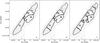 |
Fig. C.1 Results of the clumpfind decomposition. The algorithm was run with a: 1σ; b: 0.5σ and c: 0.2σ contouring stepsizes. N(H2) from Herschel and the positions of TMC-1 CP, IRAS 04381+2540, the SO peak, and our NH3 maximum are indicated as in Fig. 5a. |
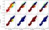 |
Fig. C.2 Best results of the other NbClust runs: HAC methods with a) McQuitty’s; b) Ward’s; c) Ward’s second; d) the complete; e) the average; f) the median; g) the centroid and h) the single criteria. N(H2) from Herschel and the positions of TMC-1 CP, IRAS 04381+2540, the SO peak, and our NH3 maximum are indicated as in Fig. 5a. The clusters in the main ridge on panel a) are numbered from M1 to M10 and discussed shortly in Sect. 4.2.3. |
Appendix C.2: K-means clustering
The k-means clustering (MacQueen 1967; Murtagh & Heck 1987) uses the centroid cluster model. It is an iterative method that minimizes the within-cluster sum of squares for a given number of clusters, starting with an initial guess for cluster centres. Each observation is placed in the closest cluster, the cluster centres are updated, and then the process repeats itself until the cluster centres no longer change.
Appendix C.3: Hierarchical clustering
The hierarchical agglomerative clustering (HAC) uses distance connectivity and seeks to build a hierarchy, where each observation starts in its own cluster, then pairs of clusters are merged according to an agglomeration criterion as one moves up the hierarchy. Another approach is hierarchical divisive clustering where all observations start in one cluster, and splits are performed recursively as one moves down the hierarchy.
The HAC methods require an agglomeration (or linkage) criterion. When building the hierarchy of clusters found in a dataset, the two clusters with the shortest distance between each other are merged at each step. The linkage criterion defines the way this between-cluster distance is measured. It can be defined, for example as the distance of the elements that are the farthest away in two clusters (complete-linkage; Sorensen 1948), the shortest distance between two elements not yet belonging to the same cluster (single; Sokal & Michener 1958), the average distance of the elements inside two clusters (average; Sokal & Michener 1958), and the squared Euclidean distance between the gravity centres of two clusters (centroid; Sokal & Michener 1958). Linkage criteria also can be determined with the weighted mean of the between-cluster distances (McQuitty; McQuitty 1966), the median of the between-cluster distances (median; Gower 1966), or with minimizing within-cluster variance (Ward and its second variant; Ward 1963; Murtagh & Legendre 2014).
Appendix C.4: The NbClust package
The R project for statistical computing provides a wide variety of the previously listed algorithms. We used the NbClust package (Charrad et al. 2014) to select the best clustering method with the most applicable input parameters to partition the TMC-1 joined Herschel/NH3 dataset into clusters. The k-means and HAC methods with eight different agglomeration criteria are both available in NbClust. The package has been developed to not only perform several types of clustering methods, but to evaluate the quality of clusters (the degree with which a clustering scheme fits a specific dataset) and the optimal number of clusters (which is a required input parameter for the algorithms) in a partitioning. This is the so-called cluster validity. For this purpose, a variety of validity measures (indices) were defined in the literature. The main benefit of using this package lies in the possibility of simultaneously evaluating several clustering schemes while varying the number of clusters. This helps to determine the
most appropriate number of clusters for the dataset, then the resulting ideal clustering scheme can be run by the same package.
One first has to define the distance measure to be used by the clustering methods. The distance measure defines how the distance of two vectors (elements or points in the dataset) are calculated during the clustering process. Euclidean distance is the usual square distance between two vectors, Manhattan distance measures the absolute distance and maximum distance is the greatest distance of two vectors. The Canberra, binary, and Minkowski distance measures are also available in NbClust (Seber 2009).
The NbClust algorithm can be run on a range of cluster numbers, choosing from the measures and methods described above, while cluster validity is assessed using the validity indices. Cluster validity (evaluating the quality of clusters, optimizing the number of clusters derived) can be described using three different approaches (Theodoridis & Koutroumbas 2006): external criteria (comparing the results to externally provided classes or labels), internal criteria (the information obtained within the clustering process is used to evaluate how well the results fit the data), and relative criteria (compares the results with other clustering schemes resulting from the same algorithm but with different parameters). Most of the validity measures determined for the third approach (Milligan & Cooper 1985; Dunn 1974; Rousseeuw 1987) were incorporated in the NbClust package. The validity indices combine information about within-cluster compactness, between-cluster isolation and other geometric or statistical properties of the data, and the number of elements and distance measures. See Charrad et al. (2014) and references therein for the detailed description of NbClust and the definitions of distance measures, linkage criteria, and cluster validity indices.
All Tables
All Figures
|
Fig. 1 Herschel N(H2) column density map of HCL 2 and the main parts of the cloud. PGCCs with flux quality of 1 and 2 are plotted with black ellipses and the numbers refer to Table 1, which lists the properties of the PGCCs. |
| In the text | |
|
Fig. 2 Typical NH3(1, 1) and NH3(2, 2) spectra on our NH3 grid. This position has the highest NH3(1, 1) optical depth from the spectra where we observed the NH3(2, 2) line as well (position #5 in Table 2). |
| In the text | |
|
Fig. 3 a): Herschel-based Tdust map of TMC-1. The numbers indicate the positions where high S/N NH3(1, 1) and (2, 2) spectra were taken and used to calculate the physical parameters of the gas (see Table 2). b) Herschel-based N(H2) map with the NH3(1, 1) main group integrated intensity contours: 0.6, 1.0, and 2.0 Kkm s-1 (20, 35, and 65% of the maximum). The secondary line components were subtracted from the spectra. Black ellipses indicate the two PGCCs in TMC-1. The positions of TMC-1 CP, TMC-1(NH3), the SO peak, and IRAS 04381+2540 are indicated with a diamond, a triangle, a square, and an asterisk, respectively. HPBW of 40″ is shown in the left bottom corner. |
| In the text | |
|
Fig. 4 Top: multiple HFS line profile fitting of NH3(1, 1) on the (−400, 520) offset. The spectrum shows one of the brightest secondary line components and gives the lowest Tkin value; see position #4 in Table 2. Box 1: single HFS line profile fit; box 2: residual from the single HFS fit; box 3: simultaneous HFS profile fitting of both components; box 4: the residual from the simultaneous HFS fit; box 5: the residual from the single HFS fit with the HFS fit of the secondary component shown in box 4. Bottom: single NH3(1, 1) HFS line profile fit on position #8 and the residual after subtracting the fit. This position has the highest HFS linewidth from the spectra in Table 2. We note the different scales for the (1, 1) and (2, 2) lines. |
| In the text | |
|
Fig. 5 a): vLSR distribution of the main (or only) line component of the NH3(1, 1) lines with S/N> 3. Circles indicate the positions where a secondary component was found and their color corresponds to the velocity of this component. b): N(NH3(1, 1)) distribution map calculated on positions where the τ optical depth from single HFS profile fit had an error of less than 50%. The grey area shows the total extension of the observed NH3 map and the grey contours are the Herschel N(H2): 0.7, 1.0, 1.3, 1.6, 2, 2.3, 2.6 × 1022 cm-2 (from 20 to 80% of the maximum by 10%). The positions of TMC-1 CP, TMC-1(NH3), the SO peak, and IRAS 04381+2540 are indicated as before and the position of our NH3 peak is indicated with an upside down triangle. |
| In the text | |
|
Fig. 6 Resulting clusters from the k-means clustering method projected back to the plane of the sky. The grey contours are the Herschel N(H2): 0.7, 1.0, 1.3, 1.6, 2, 2.3, 2.6 × 1022 cm-2 (from 20 to 80% of the maximum by 10%). The positions of TMC-1 CP, IRAS 04381+2540, the SO peak, and our NH3 maximum are indicated as before. |
| In the text | |
|
Fig. 7 Central velocity and non-thermal velocity dispersion of the NH3(1, 1) primary components along TMC-1F4 (crosses) and TMC-1F1 (circles) from left to right. The sound speed in the two clumps are indicated with a dashed line in the lower panel. |
| In the text | |
|
Fig. C.1 Results of the clumpfind decomposition. The algorithm was run with a: 1σ; b: 0.5σ and c: 0.2σ contouring stepsizes. N(H2) from Herschel and the positions of TMC-1 CP, IRAS 04381+2540, the SO peak, and our NH3 maximum are indicated as in Fig. 5a. |
| In the text | |
|
Fig. C.2 Best results of the other NbClust runs: HAC methods with a) McQuitty’s; b) Ward’s; c) Ward’s second; d) the complete; e) the average; f) the median; g) the centroid and h) the single criteria. N(H2) from Herschel and the positions of TMC-1 CP, IRAS 04381+2540, the SO peak, and our NH3 maximum are indicated as in Fig. 5a. The clusters in the main ridge on panel a) are numbered from M1 to M10 and discussed shortly in Sect. 4.2.3. |
| In the text | |
Current usage metrics show cumulative count of Article Views (full-text article views including HTML views, PDF and ePub downloads, according to the available data) and Abstracts Views on Vision4Press platform.
Data correspond to usage on the plateform after 2015. The current usage metrics is available 48-96 hours after online publication and is updated daily on week days.
Initial download of the metrics may take a while.