| Issue |
A&A
Volume 589, May 2016
|
|
|---|---|---|
| Article Number | A31 | |
| Number of page(s) | 14 | |
| Section | The Sun | |
| DOI | https://doi.org/10.1051/0004-6361/201527571 | |
| Published online | 08 April 2016 | |
Formation of a solar Hα filament from orphan penumbrae
1 Max Planck Institute for Solar System Research Justus-von-Liebig-Weg 3 37077 Göttingen Germany
e-mail:
This email address is being protected from spambots. You need JavaScript enabled to view it.
2 School of Space Research, Kyung Hee University Yongin 446-701 Gyeonggi Korea
Received: 15 October 2015
Accepted: 16 March 2016
Abstract
Aims. The formation and evolution of an Hα filament in active region (AR) 10953 is described.
Methods. Observations from the Solar Optical Telescope (SOT) aboard the Hinode satellite starting from UT 18:09 on 27th April 2007 until UT 06:08 on 1st May 2007 were analysed. 20 scans of the 6302 Å Fe I line pair recorded by SOT/SP were inverted using the spatially coupled version of the SPINOR code. The inversions were analysed together with co-spatial SOT/BFI G-band and Ca II H and SOT/NFI Hα observations.
Results. Following the disappearance of an initial Hα filament aligned along the polarity inversion line (PIL) of the AR, a new Hα filament formed in its place some 20 h later, which remained stable for, at least, another 1.5 days. The creation of the new Hα filament was driven by the ascent of horizontal magnetic fields from the photosphere into the chromosphere at three separate locations along the PIL. The magnetic fields at two of these locations were situated directly underneath the initial Hα filament and formed orphan penumbrae already aligned along the Hα filament channel. The 700 G orphan penumbrae were stable and trapped in the photosphere until the disappearance of the overlying initial Hα filament, after which they started to ascend into the chromosphere at 10 ± 5 m/s. Each ascent was associated with a simultaneous magnetic flux reduction of up to 50% in the photosphere. The ascended orphan penumbrae formed dark seed structures in Hα in parallel with the PIL, which elongated and merged to form an Hα filament. The filament channel featured horizontal magnetic fields of on average 260 G at log (τ) = −2 suspended above the nearly field-free lower photosphere. The fields took on an overall inverse configuration at log (τ) = −2 suggesting a flux rope topology for the new Hα filament. The destruction of the initial Hα filament was likely caused by the flux emergence at the third location along the PIL.
Conclusions. We present a new interpretation of the Hα filament formation in AR 10953 whereby the mainly horizontal fields of orphan penumbrae, aligned along the Hα filament channel, ascend into the chromosphere, forming seed fragments for a new, second Hα filament. The orphan penumbral fields ascend into the chromosphere ~9–24 h before the Hα filament is fully formed.
Key words: Sun: filaments, prominences / Sun: magnetic fields
© ESO, 2016
1. Introduction
Solar Hα filaments are among the longest (Deslandres 1894; Waldmeier 1938; Zirin & Tandberg-Hanssen 1960) and best studied (see reviews by Hirayama 1985; Tandberg-Hanssen 1995; Mackay et al. 2010) objects in the Sun’s atmosphere. They are easily identified as dark filaments on the disc (e.g. Lin et al. 2005) or as prominences suspended above the solar limb (e.g. Okamoto et al. 2007) when the Sun is observed in a strong spectral line such as Hα. The comparatively cool, dense material making up the bulk of the Hα filament is prevented from immediately returning to the photosphere by magnetic fields pervading it.
Photospheric magnetograms revealed that Hα filaments are typically located along a polarity inversion line (PIL; Babcock & Babcock 1955) flanked by kG magnetic field concentrations (MFCs). Running along the long axis of Hα filaments are typically hG horizontal fields (Leroy et al. 1983, 1984; Kuckein et al. 2009, 2012a; Xu et al. 2012). Beginning with the earliest Hα filament models (Kippenhahn & Schlüter 1957), the Hα filament’s material is proposed to reside in dips in the magnetic field connecting the opposite polarities on either side of the PIL. The model by Kippenhahn & Schlüter (1957) and its various extensions by Malherbe & Priest (1983), Heinzel & Anzer (2001) proposes a normal polarity configuration, whereby the magnetic field lines connect the opposite polarities flanking the PIL akin to a potential field configuration. The inverse or O-loop configuration, suggested by Kuperus & Tandberg-Hanssen (1967), Kuperus & Raadu (1974), but see also Priest et al. (1989), van Ballegooijen & Martens (1989) tends to be the favoured configuration given the variety of observations supporting it (e.g. Bommier et al. 1994; Lites et al. 1995; Dere et al. 1999; López Ariste et al. 2006; Okamoto et al. 2008; Kuckein et al. 2012a), although observations in favour of the (Kippenhahn & Schlüter 1957) model have been reported by Leroy et al. (1984). However, complicated internal motions observed within Hα filaments appear to call for even more complicated models (e.g. Schmieder et al. 1991; Berger et al. 2008; Sasso et al. 2011).
The formation process of Hα filaments is less well understood. A large number of theoretical models of this process exist. The surface models typically involve atmospheric reconnection of already emerged fields brought about by shear flows and/or inflows along the PIL (e.g. van Ballegooijen & Martens 1989; DeVore et al. 2005). Alternatively, sub-surface models employ the emergence of new, twisted flux ropes through the photosphere and into the chromosphere to form a new Hα filament (e.g. Rust & Kumar 1994; Low & Hundhausen 1995). A more complete overview on these models is given in Mackay et al. (2010).
Direct observations of Hα filament creation are comparatively rare. Gaizauskas et al. (1997, 2001) observed inflow motions of MFCs in magnetograms into a PIL over several days and Wang & Muglach (2007) observed shearing in Hα fibrils, leading to Hα filament creation and supporting the surface-type models. In contrast, Lites et al. (1995) and Okamoto et al. (2008, 2009) observed the emergence of a flux rope along a PIL also leading to Hα filament creation and supporting the sub-surface models. However, the Hα filament creation observed by Lites et al. (1995) took place in conjunction with delta sunspots, which are rarer than Hα filaments, whilst the flux emergence observed by Okamoto et al. (2008, 2009) failed to show any of the typical flux emergence signs (Cheung & Isobe 2014). The investigations by Kuckein et al. (2012b), Xu et al. (2012), whilst generally supporting the rising flux rope scenario, lacked the required temporal resolution to unambiguously characterise the evolution of their magnetic structures. The observations by Gaizauskas et al. (1997, 2001), Wang & Muglach (2007) employed low resolution data (1′′–2′′) and the necessary shear flows along the PIL have so far never been directly observed during Hα filament creation.
Given the need for further and more detailed observations on the creation of Hα filaments, we analysed active region (AR) 10953, which hosted two consecutive, well studied Hα filaments (Okamoto et al. 2008, 2009; Wheatland & Régnier 2009; Su et al. 2009; Canou & Amari 2010). The description of the evolution and the formation process of the second Hα filament is the aim of this paper.
2. Observations and Analysis
This investigation employs data sets recorded by the narrow-band filter imager (NFI), the broad-band filter imager (BFI) and the spectropolarimeter (SP), all of which are part of the Solar Optical Telescope (SOT; Tsuneta et al. 2008; Suematsu et al. 2008; Ichimoto et al. 2008; Shimizu et al. 2008) aboard the Hinode satellite (Kosugi et al. 2007). The SOT was extensively used to monitor the photospheric and chromospheric evolution of AR 10953 at a high spatial and spectral resolution. The AR was tracked from 27th April 2007 until 7th May 2007, which encompassed the AR’s passage across the solar disc. The PIL of the AR hosted successive Hα filaments. Unfortunately, the pointing of the SOT was such that beginning at the 1st of May the Hα filament was largely outside the field of view (FOV) so that data sets of the AR recorded afterwards are not included in this investigation.
The SOT/SP records two magnetically sensitive photospheric Fe I lines at 6302 Å with a spectral resolution of 30 mÅ. At each slit position the four Stokes parameters I, Q, U and V are recorded. The majority of the observations were performed using the fast mode, which is characterised by an exposure time of 1.6 s per slit position and effective pixels size of  . Three data sets at UT 09:00 and 15:00 on 28th April and UT 18:35 on 30th April were obtained in the normal mode, which has an exposure time of 4.8 s per slit position and effective pixel size of
  . Due to the different spatial sampling and exposure times both observation modes have a noise level of 1 × 10⁻³Ic. All the SOT/SP data sets used in this investigation are listed in Table 1 and are typically 3–5 h apart from each other. Each data set was reduced using sp_prep (Lites & Ichimoto 2013) and then inverted using the SPINOR code (Frutiger et al. 2000).
Analysed SOT/SP scans.
The inversion procedure follows the 2D spatially coupled inversion technique introduced by van Noort (2012), which has subsequently been applied to many SOT/SP data sets (Riethmüller et al. 2013; van Noort et al. 2013; Tiwari et al. 2013; Lagg et al. 2014; Buehler et al. 2015). The technique takes into account the local image degradation caused by SOT/SP’s point-spread-function (PSF) during the inversion procedure itself. Since the global straylight contribution in SOT/SP observations is below 10% (Danilovic et al. 2008; van Noort 2012), the central part of the PSF accounts for the bulk of the expected rms contrast in the observations. As a result the observed spectra can be successfully described in terms of a single atmosphere per pixel and the need to introduce a filling or straylight factor is removed. Spectra of the photosphere routinely display both amplitude and area asymmetries in their Stokes parameters (Solanki 1993; Stenflo 2010; Viticchié & Sánchez Almeida 2011), which are indicative of line-of-sight (LOS) gradients in the atmosphere. The fitted model atmospheres of the inversion could account for these LOS gradients through the use of three nodes in optical depth, at log (τ) = 0,−0.8 and −2. At each node the atmospheric parameters, the temperature, T, the magnetic field, B, the LOS field inclination, γ, the LOS field azimuth, φ, the LOS velocity, v, and microturbulence, ξ, could be altered. Values belonging to optical depths other than the three nodes were obtained from spline interpolations through the three nodes. By solving the radiative transfer equation using the STOPRO routines (Solanki 1987), which are part of the SPINOR code, synthetic Stokes spectra of a given model atmosphere can be generated and compared to observed spectra. Through the use of response functions and a Levenberg-Marquardt algorithm, which minimises a χ2 merit function, the atmospheric parameters of a pixel’s model atmosphere can be iteratively fitted until the synthesised spectra closely match the observed ones.
All the LOS inclinations and LOS azimuths obtained from the inversions were subsequently converted to local solar coordinates and the 180° azimuth ambiguity was removed. The azimuth ambiguity removal routine follows the principles outlined in Buehler et al. (2015) whereby the magnetic orientation of canopy pixels at log (τ) = −2 of a MFC is resolved by relating them to the core pixels of the MFC under the assumption that the magnetic field is approximately divergence free. The remaining pixels are then resolved by local dot products with already azimuth resolved pixels. In regions with high magnetic field strengths such as a sunspot the jz component of the current is additionally taken into account. Pixel with field strengths below 50 G were not resolved. The corrected inclinations and azimuths are labelled Γ and Φ respectively. The zero velocity was set by forcing the mean umbral LOS velocity to zero, which required a correction of 230 ± 50 m/s for the various SOT/SP data sets.
The spatial resolution of fast mode SOT/SP images is only  , while an individual flux tube in the form of a bright point can have a width of only
  (Lagg et al. 2010) or even less (Riethmüller et al. 2014). As a result, the magnetic field strength values obtained from the inversions should be viewed as a lower limit of the true values, in particular for smaller magnetic structures. However, this investigation focusses on magnetic fields involved in the evolution of an Hα filament surrounded by an extensive plage/pore region as well as a sunspot, all of which are structures which are generally several times the spatial resolution limit of in size. Any fine structure belonging to these magnetic fields is, nonetheless, largely lost and will only be lightly touched upon in the following sections. Finally, the inversion results support and complement the co-temporal and co-spatial SOT/BFI and SOT/NFI observations of the AR.
The BFI performed observations of the G-band at 4305 Å, which forms in the photosphere, and Ca II H at 3968 Å, which mainly depicts the upper photosphere due to the broadness of the employed filter (Carlsson et al. 2007). The BFI observations possess the highest angular resolution at  . The NFI observed the AR in the Hα line at 6563 Å with an angular resolution of . The Hα observations suffer from an air bubble, which obscures and distorts part of the image and places an observable intensity pattern across the remaining image. Fortunately, the Hα filament investigated in this study was located far from the air bubble, allowing its evolution to be monitored continuously. All three channels performed observations of the AR with a cadence of one image per minute starting at UT 11:39 on 28th April 2007 until UT 06:07 on 1st May 2007, except for small gaps of 15 min every 2–3 h. All three channels were reduced using fg_prep. The observations overlap with the SOT/SP scans save for the initial two in Table 1. The BFI, NFI and SP observations were aligned to each other using a rigid alignment routine available from the solarsoft package.
3. Results
A general impression of AR 10953’s evolution can be gained from Fig. 1, which depicts the temperature at log (τ) = 0 of four different SOT/SP scans. At UT 11 on 28th April the AR harbours a fully developed sunspot surrounded by pores and orphan penumbrae. By UT 02 on 1st May many of these surrounding structures have disappeared and the AR appears to have lost some of its complexity. Three regions, enclosed by the boxes A, B and C, undergo the greatest change in time and play a critical role in the formation of the AR’s Hα filament.
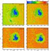 |
Fig. 1 Temperatures at log (τ) = 0 from the inversion of four SOT/SP scans. The colour bar applies to all plots. The xy axes indicate the distance to disc centre. The three boxes marked A, B and C enclose regions of rising flux. |
The evolution of the magnetic field strengths is shown in Fig. 2. The two rows indicate the fields at the upper two log (τ) nodes set during the inversion. At UT 11 on 28th April regions A, B and C all contain kG fields across all three log (τ) layers, which match the locations of reduced temperature seen in Fig. 1. As the three regions evolve, the kG fields give way to a more diffuse hG field (light blue colour in Fig. 2), which is prevalently situated in the upper node at log (τ) = −2. It is nestled between the MFCs aligned along the PIL and is suspended above the photosphere, since the corresponding lower log (τ) layers are almost field free.
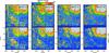 |
Fig. 2 Magnetic field strengths obtained from the inversions. Each column corresponds to a separate SOT/SP scan, and the upper and lower rows indicate the field strengths at log (τ) = −2 and –0.8 respectively. The colour bar applies to all plots and the xy axes indicate the distance to disc centre. The three white boxes are identical to those in Fig. 1. |
Figure 2 also reveals that regions A, B and C do not evolve simultaneously but separately. Region C is the first to evolve and by UT 18 on 28th April (Col. 2 Fig. 2) hosts a hG field suspended at log (τ) = −2. Regions A and B initially remain relatively unchanged, but eventually follow suit and also host their suspended hG field by UT 11 on 29th April (Col. 3 Fig. 2), some 17 h later. Note that, at this time the hG fields of the three regions are still separated from each other by several kG MFCs (e.g. −470X, −100Y). The separate hG field regions continue to expand (see Col. 4 Fig. 2) and by UT 13 on 30th April the hG fields form a continuous channel.
Figure 3 displays the inclination of the magnetic fields at log (τ) = −2, while the black contour lines encompass kG MFCs. The presence of an extended plage region of opposite polarity to the sunspot can be discerned from this figure. Regions A, B and C are all placed on the PIL running through the AR (see white line at e.g. UT 01 on 30th April in Fig. 3 for reference). Even though the magnetic fields in regions A, B and C evolve in time, the PIL is maintained throughout. Aligned along the PIL are MFCs, which is characteristic for most Hα filament channels. The MFCs on the sunspot side are, furthermore, affected by the Sunspot’s moat flow, which carries new MFCs towards the PIL (Okamoto et al. 2009; Vargas Domínguez et al. 2012). The lower row panels in Fig. 3 illustrate this behaviour. Whilst the MFCs around the PIL contain predominantly vertical fields, the fields on the PIL itself are predominantly horizontal, especially once regions A, B and C have reduced in complexity. Furthermore, the azimuthal orientation of this field, displayed by the arrows in Fig. 3, follows an inverse configuration (i.e. the field also points from negative to positive polarity) at e.g. UT 01 on 30th April once the three regions have merged.
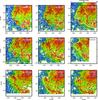 |
Fig. 3 LOS inclinations at log (τ) = −2 of four SOT/SP scans. The black contour lines indicate kG magnetic fields at log (τ) = −0.8. The colour bar applies to all panels, where blue represents positive polarity fields and red the negative polarity. The arrows indicate the direction of the azimuthal magnetic field component at log (τ) = −2 and the white line follows the PIL. The xy axes indicate the distance to disc centre. The three white boxes are identical to those in Fig. 1. |
The horizontal hG field aligned along the PIL at UT 13 on 30th April in Figs. 2 and 3 indicates the presence of an Hα filament suspended above the photosphere. The SOT/NFI observations displayed in Fig. 4 not only support this assertion, but also reveal that the complex photospheric evolution seen in Figs. 1–3 is mirrored in the chromosphere. The observations show that a fully formed Hα filament was already present above the PIL at UT 11:50 on 28th April, which is near the start of the SOT/NFI observation run. Furthermore, the photospheric magnetic fields of regions A and B are situated directly underneath the Hα filament, whereas region C is slightly offset. The initial Hα filament is stable until a series of small dynamic brightening events rooted at region C (e.g. 45X,20Y at UT 21:34, 21:50 on 28th April in Fig. 4) begin to erode it. The events manifest themselves in the form of intense brightenings lasting no longer than two images (<2 min), which are seen simultaneously in Hα and Ca II H. They may be a manifestation of reconnection. By UT 00:22 on 29th April the initial overlying Hα filament has disappeared and given way to several disjointed dark fragments, located at regions A, B and C. The azimuthal magnetic field component (see Fig. 3) is always orientated in parallel with these fragments. The small fragments slowly elongate to coalesce into a continuous Hα filament, by UT 20:04 on 29th April, a development that is supported by the inversion results in Figs. 2 and 3. The newly formed Hα filament then remains stable until at least the 7th of May, although a few sporadic brightening events do occur along the PIL.
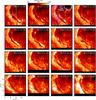 |
Fig. 4 Sequence of SOT/NFI Hα images. The colour bar applies to all plots and the xy axes indicate the size of each image. The contour lines in the 3rd frame of the top row enclose kG magnetic fields at log (τ) = −0.8 obtained from the inversion of a SOT/SP scan. The grey contour lines in the third panel of the top row correspond to negative polarity and the magenta to positive polarity fields. The three white boxes are identical to those in Fig. 1. |
The evolution of the PIL and the Hα filaments located within it appears to be driven by the magnetic fields in regions A, B and C. Region C appears to be responsible for the destabilisation of the initial Hα filament as well as providing one of the seeds from which the new Hα filament is formed. Regions A and B, while comparatively passive at first, also appear to be intimately involved in the creation of the new Hα filament. Therefore, the three regions will be examined more closely.
3.1. Region C
Region C is the southernmost region of the three and was outside the FOV of the SOT/BFI channels at all times. Due to the continuous northward drift of the FOV of all SOT channels, the majority of region C was also outside the FOV of the SOT/SP and Hα channels by UT 09 on 30th April (see Figs. 2 and 3). The first SOT/SP scan at UT 18 on 27th April already shows the existence of the PIL, but contains no magnetic structure that can be linked to the pore situated at the heart of region C at UT 11 on 28th April (see Fig. 1), suggesting that region C is composed of freshly emerged flux. The second SOT/SP scan at UT 09 on 28th April hints that region C already contained a pore at that time, however, a tracking error meant that the region was not scanned in its entirety. Therefore, the emergence of the magnetic flux of region C into the photosphere is unfortunately not covered by SOT.
The subsequent evolution of region C as seen by SOT/SP is displayed in Fig. 5 and corresponds to SOT/SP scans 3–5 in Table 1. At UT 11 on 28th April the temperature at log (τ) = 0 displays a dark pore at the centre of the FOV composed of kG magnetic fields in all log (τ) layers. A somewhat less dark elongated structure, around 6X,5Y, is located immediately below it. The contour lines in Fig. 5 reveal that this structure is located in between two kG magnetic field patches of opposite polarity and is itself host to horizontal fields of up to one kG. Over the two subsequent SOT/SP scans, covering 7 h, the two opposite polarity kG patches drift apart from each other and reduce in size. The magnetic flux reduces by 50% in all log (τ) layers from 9 × 10¹⁹ Mx to 4.5 × 10¹⁹ Mx at log (τ) = −0.8. Simultaneously the horizontal fields connecting the kG patches, indicated by the arrows in Fig. 5, drop form ~1 kG in all log (τ) layers to <100 G in the lower two layers (see Fig. 2) leaving a canopy field of ~260 G at log (τ) = −2. This canopy field persists in all subsequent observations (see Fig. 2).
At UT 15 on 28th April an upflow, co-spatial with the horizontal magnetic fields (7X,5Y in Fig. 5), can be seen between the two separating polarities in log (τ) = −2. The upflows reach a peak LOS velocity of 2 km s-1. The configuration of upflows at the apex of rising magnetic fields together with downflows at their foot points supports the rising flux scenario. The dark fibrils seen in Hα at UT 11 and 15 in Fig. 5 are generally orientated perpendicular to the photospheric fields, but beginning at UT 18 (5X,3Y in Fig. 5) at the location of the earlier photospheric upflows small fibrils connecting the opposite kG polarities and orientated in parallel with the photospheric field can be spotted. The photospheric fields and Hα fibrils remain aligned for as long as region C can be identified (see Figs. 2–4).
Furthermore, the azimuthal orientation of region C’s magnetic fields after they rose into the chromosphere already display an inverse configuration at log (τ) = −2 at UT 03 on 29th April in Fig. 3. Together with the average field strength of 260 G and the co-spatial and aligned dark fibril seen at 55X,15Y at the same time in Fig. 4, reveal that region C alone already displays the characteristics of the Hα filament that forms out of regions A, B and C at UT 20:04 on 29th April. Potentially, magnetic fields stemming from a small, compact region such as region C may already be sufficient to form a small Hα filament.
3.2. Region B
Region B is the most striking and revealing region of the three. Its initial photospheric composition is characterised by pores and several elongated filamentary structures, which are reminiscent of orphan penumbrae. They are identifiable at UT 11 on 28th April in Fig. 1. All of these features are already fully formed in the first SOT/SP scan at UT 18 on 27th April, which indicates that the emergence of region B’s magnetic flux into the photosphere occurred when the AR was still located on the far side of the Sun.
From UT 11:39 on 28th April onwards region B was continuously monitored by SOT/NFI and the two SOT/BFI channels. The Hα images in Fig. 4 indicate that the photospheric magnetic structures of region B are located directly underneath the initial Hα filament. Whilst the initial Hα filament is in place the photospheric magnetic structures of region B are very stable (see UT 11 and 18 on 28th April in Fig. 2). Once the initial Hα filament has disappeared the photospheric composition of region B begins to change according to Figs. 2 and 4. The G-band and Ca II H observations of region B support this assertion and a selection of images of both channels is displayed in Fig. 6.
The images in Fig. 6 give an account of the photospheric evolution of region B beginning just after the disappearance of the initial overlying Hα filament. At UT 23:58 on 28th April both channels observed a pore and several orphan penumbrae connecting opposite polarities, derived from co-temporal SOT/SP observations. Over the following 8 h the orphan penumbrae become brighter and shorter before they disappear entirely leaving only the pore. These orphan penumbrae were already identifiable in the first SOT/BFI images at UT 11:39 on 28th April and the evolution of their G-band mean intensity is displayed in Fig. 7. The thick solid curve represents a 3 h smoothing of the individual mean intensity measurements and testifies to the initial stability of the orphan penumbrae followed by a gradual brightening. The dashed vertical line in the same figure marks the disappearance of the initial overlying Hα filament. Therefore, Fig. 7 indicates that the gradual evolution and disappearance of the photospheric structure is triggered by a change in the overlying chromosphere.
The individual mean intensity measurements shown by the dots in Fig. 7 display a somewhat erratic behaviour, which is principally caused by the continuous drift of the FOV of SOT/BFI and causes the orphan penumbrae to be partially outside the FOV for short periods of time. The solid line centred at 0.62 Ic in Fig. 7 represents a 3 h smoothing of the sunspot’s disc-side penumbra’s mean intensity from the same G-band observations. As expected, the sunspot penumbra remains stable throughout the observations and is considerably darker than the orphan penumbra in region B. The brightness difference appears to be largely intrinsic, since no matter how the orphan penumbra in region B is selected it is never as dark as the sunspot penumbra. The final selection of region B’s orphan penumbra was performed by drawing simple box around it, whose size is manually adjusted depending on the length and width of the structure. Each G-band image was also normalised to its own quiet Sun mean intensity to remove the limb darkening effect. A similar mean intensity evolution of the orphan penumbrae can also be observed for the Ca II H images over the same time period.
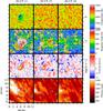 |
Fig. 5 Sequence of inverted SOT/SP scans and Hα images of region C. The purple contour lines correspond to negative polarity and the turquoise to positive polarity kG fields at log (τ) = −0.8. The arrows indicate the direction of the azimuthal magnetic field component at log (τ) = −2. The colour bars apply to all plots of their type and the xy axes indicate the size of each plot. The log (τ) layer of each plot is also indicated on the right of each row. |
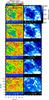 |
Fig. 6 Left: sequence of SOT/BFI G-band images of region B. Right: sequence of co-spatial and co-temporal SOT/BFI Ca II H images. The contour lines enclose kG magnetic fields at log (τ) = −0.8 obtained from inversions of SOT/SP scans. The purple contour lines correspond to negative polarity and the turquoise to positive polarity fields. The colour bars apply to all their respective images and the xy axes indicate the size of each image. |
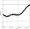 |
Fig. 7 Evolution of the SOT/BFI G-band normalised mean intensity of the orphan penumbrae displayed in Fig. 6. The dots are the individual measurements for each image and the thick solid line represents a 3 h smoothing of these measurements. The continuous thin solid line indicates a 3 h smoothing of normalised mean intensity measurements of sunspot penumbra. The vertical dashed line marks the time of the overlying Hα filament’s disappearance. |
The SOT/SP inversions compiled in Fig. 8 support and extend the impressions gained from Figs. 6 and 7 and detail the evolution of region B as obtained from the inversion of SOT/SP scans 6–11 in Table 1. The temperature plots at log (τ) = 0 in Fig. 8 contain the same orphan penumbra around 8X,8Y. Just as in Fig. 6, by UT 08 on 29th April the orphan penumbra is no longer identifiable in the temperature plots in Fig. 8. Furthermore, the pore located at the head of the orphan penumbra has also disappeared by UT 15 on 29th April. The number of kG features decreases sharply over the 18 h period covered in Fig. 8 with the consequent decrease in magnetic flux plotted in Fig. 9. Whilst the magnetic flux is close to constant over the first two time steps when the initial overlying Hα filament was still intact, it rapidly decreases following the filament’s disintegration. All the log (τ) layers reveal a similar drop of ~40% in magnetic flux over time between UT 00 and UT 15 on 29th April.
The orphan penumbra, enclosed by a white box in Fig. 8, contain generally sub-kG fields at all times, except for a few pixels at log (τ) = 0. For as long as the orphan penumbra is visible in the log (τ) = 0 temperature plots, it contains sub-kG magnetic fields across all log (τ) layers. In particular the fields at log (τ) = 0 and −0.8 closely follow the shape of the orphan penumbrae as seen in the temperature. By UT 03 on 29th April the orphan penumbra has become somewhat shorter in length and this is reflected in the magnetic fields in the lower two log (τ) layers. From UT 08 on 29th April onwards the magnetic field has almost vacated the lower two log (τ) layers and is predominantly situated in the upper log (τ) layer. The change in the mean horizontal magnetic field strength of the pixels enclosed by the white box in Fig. 8 across all log (τ) layers is plotted in Fig. 9 as well. The mean horizontal field strength at log (τ) = −2, represented by the dashed line in Fig. 9, settles at 260 G, forming a canopy over the lower two log (τ) layers.
The magnetic field inclinations in Fig. 8 demonstrate that the orphan penumbra is composed of predominantly horizontal fields, which connect opposite polarity kG MFCs. The negative polarity pore located at 5X,12Y in Fig. 8 forms the head of the orphan penumbrae, whilst its tail is formed by several small MFCs located around 13X,5Y. Once the overlying Hα filament has disappeared the two opposite polarities move apart beginning at UT 00 on 29th April. The separation of the polarities, also seen in Fig. 6, suggests that the horizontal fields between them, originally forming the fields of the orphan penumbra, are rising into the chromosphere (as described in e.g. Strous et al. 1996; Lites et al. 1998; Strous & Zwaan 1999; Centeno 2012). Unlike region C, the rise of the orphan penumbrae in region B does not cause a series of intermittent brightenings visible in the Hα and Ca II H data sets.
The orientation of region B’s orphan penumbra relative to the PIL (i.e. where Γ ~ 90°) undergoes a considerable evolution over time. From Fig. 8 it is evident that the orphan penumbra, while it is identifiable in the log (τ) = 0 temperature images (e.g. UT 21 on 28th April), is aligned in parallel with the azimuthal magnetic field component. The azimuthal component in turn is orientated in a normal configuration with respect to the PIL (also see Fig. 3). However, at UT 03 on 29th April and before, Figs. 2–4 reveal that the orphan penumbra and its field is also already aligned in parallel to the initial Hα filament as well as the Hα filament that forms by UT 20:04 on 29th April. The successive SOT/SP scans depicted in Fig. 8 indicate the aforementioned loss of magnetic flux over time (see also Fig. 9), which causes the PIL in Fig. 8 to rotate in particular from UT 11 to 15 on 29th April. The azimuthal orientation of the orphan penumbra remains comparatively stable by comparison. Hence, the azimuthal orientation of the orphan penumbra relative to the PIL appears to rotate by up to 90° over time. Note however, that the flux vacated the lower log (τ) layers already several hours before the apparent rotation.
The LOS velocities in Fig. 8 indicate fast flows in the orphan penumbra for as long as it is discernible in the log (τ) = 0 temperature layer. At all times and across all log (τ) layers the flows are co-spatial with the horizontal magnetic field of the orphan penumbra. The horizontal magnetic field at log (τ) = −2 is distributed over a greater area than at log (τ) = 0, particularly at UT 03 on 29th April, which is also reflected in the area covered by the high LOS velocities. Whilst at log (τ) = 0 the flow often appears to stop short of reaching the opposite polarity kG MFC, forming the tail of the orphan penumbrae, it does reach the opposite MFC in the log (τ) = −2 layer. Therefore, the flow appears to be partially channelled above the photosphere during the structure’s rise into the chromosphere, which may play a role in supplying mass to the forming Hα filament. The flow stops abruptly in all the SOT/SP and SOT/BFI observations once the orphan penumbra’s horizontal field has vacated the lower two log (τ) layers.
Comparison between region B’s orphan penumbra and sunspot penumbra at UT 00 29th April.
Table 2 provides a quantitive comparison between region B’s orphan penumbra and a similarly orientated part of the sunspot’s penumbra at UT 00 on 29th April (e.g. see −500X,−40Y at UT 03 on 29th April in Figs. 1 and 3). Each value represents a spatial average over each structure as identified by the temperature layer at log (τ) = 0. Table 2 reveals several quantitative differences between region B and the sunspot penumbra. Region B is consistently hotter by ~200 K across all log τ layers, in line with the persistent continuum intensity difference between the two structures shown in Fig. 7. The magnetic field strengths, too, are lower in region B by ~500 G. The LOS inclinations and azimuths are very similar, as expected from the selection criteria for both regions. The LOS velocities are of similar magnitudes, but the log (τ) layer containing the highest average flows does differ. Region B’s orphan penumbra features consistently faster flows in the upper two log (τ) layers when compared to the sunspot penumbra and, together with the lower magnetic field strengths, might indicate that it is geometrically located higher in the solar atmosphere than the sunspot penumbrae. Nonetheless, the clear spine/inter-spine structure of the orphan penumbra in region B, displayed in Fig. 6 and in all the inversion parameters listed in Fig. 8 are in keeping with the standard penumbral filament described by Tiwari et al. (2013).
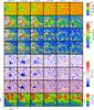 |
Fig. 8 Sequence of inverted SOT/SP scans of region B. The black contour lines enclose kG magnetic fields at log (τ) = −0.8 and the arrows indicate the direction of the azimuthal magnetic field component at log (τ) = −2. The colour bars apply to all plots of their type and the xy axes indicate the size of each plot. The log (τ) layer of each plot is also indicated on the right of each row. The white box encloses rising magnetic fields. |
For as long as the orphan penumbra in region B is identifiable in the G-band and Ca II H images (see Fig. 6) both channels also reveal several bright spines separated by comparatively darker inter-spines in the orphan penumbrae e.g. around 5X,6Y at UT 23:58 on 28th April in Fig. 6. Along the spines small bright points can be made out, which travel continuously from the pore to the structure’s tail. Bright points seen in the G-band images generally display the same behaviour except for bright points located within 3′′ of the pore and at the head of the orphan penumbra, which show an apparent counterflow directed towards the pore. In the Ca II H images these small bright points can be traced at all times and travel the entire way to the tail’s opposite polarity patch, which is situated at the lower edge of the FOV and encompassed by the turquoise contour lines in Fig. 6. By manually tracking 10 bright points they were found to have a typical plane of the sky velocity of 1.7 km s-1 in the Ca II H images at UT 03:25 on 29th April (see Fig. 6). Furthermore, the Ca II H observations support the suggestion made by Fig. 8 that during the final ascent stages at UT 03 on 29th April part of the flow in the orphan penumbrae appears to be channelled above the photosphere.
Finally, an estimate of the rise speed of the orphan penumbra through the photosphere can be obtained by combining the rise time of ~8 h displayed in Fig. 7 and taking a value of ~300 km for the thickness of the photosphere, which can be obtained from contribution functions of the 6302 Å line pair calculated by STOPRO. The resultant rise speed amounts to 10 ± 5 m/s. Therefore, the LOS velocities in the orphan penumbrae primarily depict a flow orientated in parallel to the solar surface akin to the Evershed flow (Evershed 1909). A similar conclusion about the flow direction can be gleaned by combining the bright point velocity in the Ca II H observations and the LOS velocity observations in Fig. 8.
3.3. Region A
Region A is by far the most complex region of the three. The complexity is caused by the region’s vicinity to the sunspot, the multitude of pores it harbours and the presence of a large orphan penumbra. The characteristic features of region B can also be observed for region A, some of them in a more striking fashion.
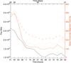 |
Fig. 9 Black: change in magnetic flux at log (τ) = −0.8 in the region covered by Fig. 8. Orange: change in mean horizontal magnetic field strength within the white box in Fig. 8. The dashed line depicts log (τ) = −2, whereas the solid and dotted lines correspond to log (τ) = −0.8 and 0, respectively. |
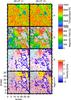 |
Fig. 10 Sequence of inverted SOT/SP scans of region A. The purple contour lines correspond to negative polarity and the turquoise to positive polarity kG fields at log (τ) = −0.8. The colour bars apply to all plots of their type and the xy axes indicate the size of each plot. The log (τ) layer of each plot is also indicated on the right of each row. |
The orphan penumbra in region A also begins to evolve once the initial Hα filament has disappeared, but it evolves somewhat slower than region B’s orphan penumbra. Two SOT/SP scans of region A revealing a similar evolutionary stage as region B at UT 03 on 29th April are presented in Fig. 10. They correspond to SOT/SP scans 10 and 11 in Table 1. The orphan penumbra is located around pixel 20X,25Y and the edge of the sunspot penumbra around 30X,30Y in Fig. 10. The temperature and magnetic field contours reveal that part of the orphan penumbra in region A is aligned in parallel to the Hα filament channel. The magnetic fields at log (τ) = −2 extend continuously from the orphan penumbrae into the PIL, forming a hG field canopy (see Fig. 2). The orphan penumbra, excluding the pores and MFCs, loses 30% of its magnetic flux between UT 00 and UT 15 on 29th April from 1.1 × 10²⁰ Mx to 8 × 10¹⁹ Mx at log (τ) = −0.8. However, an exact measure of the lost magnetic flux due to the rise of the orphan penumbra is difficult to determine given that many MFCs move considerable distances in the area of interest.
The orphan penumbra in Fig. 10 hosts fast LOS velocities, the majority of which are akin to the Evershed flow in the sunspot penumbra also displayed in the figure. Unlike region B’s orphan penumbra, the sunspot penumbra and orphan penumbra in Fig. 10 both display the fastest downflows at their tails across all log (τ) layers. At log (τ) = −2 the downflows extend beyond the orphan penumbrae’s log (τ) = 0 temperature boundary and into the PIL. The extended outflow, located at 10X,20Y, is traceable in both SOT/SP scans displayed in Fig. 10 and represents a qualitatively similar case as the one seen at UT 03 on 29th April in Fig. 8. Underneath the extended outflow a typical granulation pattern can be seen in the lower log (τ) layers.
The extended outflow in region A at UT 11 on 29th April appears to return to the photosphere along two positive polarity MFCs situated at 5X,4Y and 8X,1Y. Around the two MFCs at log (τ) = −2 the downflows are spatially extended, asymmetric and face the outflow of the orphan penumbra of region A. They are traceable in the lower two log (τ) layers as well and reach a peak velocity of 6.6 km s-1 at log (τ) = 0. Also, the two MFCs are ~200 K hotter in the upper two log (τ) layers when compared to other nearby MFCs. The Ca II H observations features persistent brightenings at the location of the MFCs. In Fig. 10 and the Ca II H observations the two MFCs are seen to recede away from the orphan penumbra over time indicative of rising magnetic fields. The orphan penumbra’s outflow would, therefore, cover a distance of ~30” and flow along the PIL. Both the extended outflow of the orphan penumbra is traceable in the Ca II H observations of region A by the movement of small bright points. The extended outflows appear to be a characteristic property of ascending orphan penumbrae.
4. Discussion
The evidence presented in Sect. 3 allows us to surmise that the formation process of the Hα filament formed by UT 20:04 on 29th April 2007 in AR 10953 is driven by the rise of horizontal magnetic fields from the photosphere into the chromosphere. In this section we compare and contrast our findings to the literature.
The investigation by Okamoto et al. (2008) employed Milne-Eddington inversions of SOT/SP data sets 10, 11, 12, 14, 17 and 20 from Table 1, to infer the rise of a helical flux rope along the PIL of AR 10953. In particular, the authors focussed on a FOV encompassing region B and parts of region C. According to the employed SOT/SP data sets the emergence is proposed to occur from UT 11 on 29th April until UT 02 on 1st May. However, the horizontal magnetic fields in both regions rose into the chromosphere before UT 11 on 29th April, some 11 h earlier for region B and 24 h for region C (see Figs. 5 and 8). The Hα filament, seeded by the horizontal magnetic fields of regions A, B and C, reformed by UT 20:04 on 29th April (see Fig. 4), making the emergence time-line proposed by Okamoto et al. (2008) irreconcilable with both the SOT/SP and SOT/NFI observations.
The helical flux rope emergence proposed by Okamoto et al. (2008) is supposed to occur simultaneously along the entire PIL, whilst leaving no discernible sign in the continuum images. Flux emergences of order of 1 ×10¹⁹ Mx or more typically produce elongated granules (Centeno 2012; Vargas Domínguez et al. 2014) or dark filamentary structures (Strous et al. 1996; Lites et al. 1998; Strous & Zwaan 1999; Kubo et al. 2003) visible in the continuum, which were not reported by Okamoto et al. (2008) over the proposed time frame. Flux emergence even at the smallest scales (Centeno et al. 2007; Danilovic et al. 2010) always entails an increase in magnetic flux, which is not supported by the SOT/SP observations in Sect. 3 nor by SoHO/MDI observations of AR 10953 (Vargas Domínguez et al. 2012). In addition, magneto-hydrodynamic (MHD) simulations of flux rope emergence reveal that the magnetic field emerges in a piecemeal fashion and at several locations, after it has been distorted by and subjected to the solar convection (Cheung et al. 2007, 2008, 2010; Martínez-Sykora et al. 2008; Stein & Nordlund 2012). MHD simulations, where a horizontal flux rope emerged along the entire length of the simulation box, still displayed an initial increase in magnetic flux and deformations in the granules (Yelles Chaouche et al. 2009; MacTaggart & Hood 2010). Regions A, B and C all contain structures visible in the continuum typical of flux emergence. They may represent the individual flux emergence sites of a larger connected flux system rising through the photosphere.
Okamoto et al. (2008) observed a rotation in the magnetic field’s azimuthal direction with respect to the PIL of almost ~50° from UT 11 on 28th April until UT 02 on 1st May. The field appears to turn from an initially normal to finally an inverse configuration, even though the horizontal magnetic fields of both region B and C have already risen into the chromosphere by that time. The observed azimuth rotation is, therefore, a spurious effect brought about by the decay of magnetic flux in region B, which continued for some time after the horizontal field’s ascend (see Fig. 9). The decay of flux locally effected a rotation of the PIL itself rather than in the azimuth of the magnetic field (see UT 11 and 15 on 29th April in Fig. 8). Furthermore, the azimuthal orientation of region C’s horizontal magnetic fields, which ascended into the chromosphere some 24 h before UT 11 on 28th April (see Fig. 2 and 5), are displayed in the lower right hand corner of Fig. 2’s FOV in Okamoto et al. (2008). They exhibit an inverse configuration throughout the time-line used by Okamoto et al. (2008), which defies their proposed scenario.
The sliding door mechanism, a widening followed by a narrowing of the PIL, was proposed by Okamoto et al. (2008) as evidence and photospheric signature for a magnetic flux rope that rises through the photosphere and into the corona. It occurs at the same time as the azimuth rotation. Since our investigation uses the same SOT/SP data sets, the sliding door mechanism can also be seen in, for example, Fig. 3. However, in light of the evidence presented in Sect. 3, the sliding door mechanism cannot be a sign of flux emergence. It appears to be a combination of flux decay (see Figs. 3, 8 and 9), which caused a widening of the PIL, and the continuous moat flow around the sunspot (see Fig. 3 and Okamoto et al. 2009; Vargas Domínguez et al. 2012), which slowly pushed new MFCs into the PIL, hence causing it to narrow. In the Ca II H observations the widening of the PIL is seen as a growing dark area (see Fig. 1 in Okamoto et al. 2009), in line with a decay of kG MFCs. The subsequent narrowing of the PIL manifests itself by a reduction of the dark area, by encroaching bright kG MFCs. The narrowing of the PIL (see Fig. 1 in Okamoto et al. 2009) is greatest at the sunspot-facing side of the PIL in keeping with a moat flow-aided replenishment of MFCs to the PIL.
The average photospheric magnetic field strength of 260 G at log (τ) = −2 in the filament channel at UT 20:04 on 29th April (see Fig. 4), when the new Hα filament has formed, is consistent with previous such measurements (Lites 2005; Okamoto et al. 2008; Lites et al. 2010; Xu et al. 2012; Sasso et al. 2014). At several locations within the PIL higher fields strengths of up to 800 G at log (τ) = −2 can be observed, which appear to be somewhat short lived, since they can never be observed at the same place in consecutive SOT/SP scans. Similarly high magnetic field strengths in Hα filaments have been previously reported both in chromosphere (Kuckein et al. 2009; Sasso et al. 2011) and photosphere (Kuckein et al. 2012a).
The Hα filament created by UT 20:04 on 29th April coincides with horizontal magnetic fields at log τ = −2, whose azimuthal component is predominantly aligned in parallel with the PIL, but also appears to point from negative to positive magnetic polarity (see Fig. 3). This highly non-potential configuration of the azimuthal magnetic field component is commonly referred to as an inverse configuration, which has also been noted by Okamoto et al. (2008) for the same Hα filament and has been observed in many other cases (e.g. Lites 2005; López Ariste et al. 2006; Kuckein et al. 2012a). The inverse configuration has been commonly interpreted as the photospheric observable of a chromospheric horizontal flux rope (e.g. Priest et al. 1989).
Kuckein et al. (2012a) observed orphan penumbrae aligned in parallel to the Hα filament channel hosting an Hα filament at various times. The supersonic downflow velocities located at the edges of their orphan penumbrae (Kuckein et al. 2012b), appear to be akin to the high downflows seen in region A at the tails of the orphan penumbra and sunspot penumbra (see Fig. 10). The orphan penumbrae are interpreted as parts of an extremely low lying filament trapped in the photosphere. Although their orphan penumbrae also subsequently disappear, it is unclear from the available observations, whether they played a similar role as the orphan penumbrae described in Sect. 3.
Region C (see Fig. 5) displays properties akin to a rising loop system (Solanki et al. 2003; Lagg et al. 2004; Xu et al. 2010) during its initial rise into the chromosphere. The brightening events leading to the eventual disappearance of the initial Hα filament (see Fig. 4), suggests an interaction and possible reconfiguration of the pre-existing chromospheric fields and the rising fields (Manchester et al. 2004; Archontis et al. 2013). However, regions B and A do not show similar brightening events and instead the photospheric observations (see Figs. 8 and 10) indicate that the orphan penumbra wholly rises into the chromosphere.
The investigations by Guglielmino et al. (2014), Zuccarello et al. (2014) analysed orphan penumbrae similar to regions A and B and concluded that they are a manifestation of emerged Ω loops, which are trapped in the photosphere. The evolution of region B in particular both supports and complements their findings. The orphan penumbra in region B is stable for at least 12 h, whilst located underneath the initial Hα filament. Once the overlying Hα filament and, presumably, most of its horizontal magnetic field have disappeared the orphan penumbra can no longer be maintained in the photosphere and begins to ascend (see Fig. 7). Furthermore, the sunspot penumbra formation process studied by Shimizu et al. (2012), Rezaei et al. (2012), Lim et al. (2013), Jurčák et al. (2014a) indicates that sunspot penumbra formation only sets in after a sufficient horizontal magnetic field has been established within the overlying chromosphere. We speculate that there is a similar need for strong overlying chromospheric fields to form and maintain orphan penumbrae.
Jurčák et al. (2014b) performed a comparison between orphan and sunspot penumbrae and found many qualitative similarities, but, like region B, the orphan penumbrae featured higher intensities and higher Evershed-like velocities (see Table 2). The orphan penumbrae studied by Jurčák et al. (2014b) submerged over time unlike the orphan penumbrae in regions A and B, which ascended into the chromosphere. Sub-photospheric processes are likely responsible for this divergent evolution.
Delta sunspots are often associated with producing and hosting Hα filaments (Tanaka 1991; Gaizauskas et al. 1994; Leka et al. 1996; Lites & Low 1997). The penumbra between the two opposite polarity umbrae is usually aligned in parallel to the PIL. Their large size allows a detailed analysis of their horizontal fields even when only a spatial resolution of 1′′ is available. Lites et al. (1995) observed the emergence and decay of a delta sunspot, which was accompanied by the formation of an Hα filament. The observations were interpreted as an ascent of horizontal fields from the photosphere into the chromosphere, thereby forming an Hα filament. The evolution of the whole system shares many analogies with regions A, B and C such as, penumbra aligned with the PIL, persistent high/supersonic LOS velocities in the penumbra (Martínez Pillet et al. 1994), magnetic flux decay during and after the ascend of the horizontal fields, little flaring activity during the ascent, and a remaining Hα filament after large photospheric structures have been largely reduced to plage MFCs. The qualitative similarities between the results in Sect. 3 and those of Lites et al. (1995) suggest that our observations may represent a scaled down version of the same overall process (Rust & Kumar 1994).
Martin (1990) proposed a series of six conditions, which would automatically lead to the creation of an Hα filament. The Hα filament formation described in Sect. 3 supports the conditions proposed by her, although the original conditions did not include rising/emerging flux. The AR features a PIL that exists throughout the entire observation runs and supports an overlying coronal arcade. The coronal arcade has not been shown explicitly here, but has been independently observed and extrapolated by De Rosa et al. (2009). It has also been extrapolated by Wheatland & Régnier (2009). The magnetic fields within the PIL are transverse in the photosphere (see Fig. 3) and the initial Hα filament as well as the individual fragments, which precede the fully formed Hα filament, are all aligned parallel to the PIL (see Fig. 4), in accord with Martin (1990). The two key proposed photospheric observables leading to Hα filament creation, are a continuous advection of small MFCs into the PIL (Gaizauskas et al. 1997, 2001) and their cancellation presented as flux decay (Lites et al. 1995). Whilst the PIL in AR 10953 experiences a continuous advection of fresh MFCs into the PIL by the sunspot’s moat flow (Okamoto et al. 2009; Vargas Domínguez et al. 2012), the magnetic structures in regions A, B, and C involved in the formation of the Hα filament were already present before the start of the observation runs. The photospheric flux decay, however, is observed for all three regions and in keeping with Martin (1990). Since the conditions proposed by Martin (1990) were based on low resolution (1′′−2′′) filtergram data and LOS magnetograms, we can add to the proposed conditions that the flux decay is, at least in this case, initially accompanied by rising horizontal magnetic fields. Two of the three additional criteria added by Martin (1998) can be verified in our observations as well. The SOT/NFI Hα and SOT/BFI Ca II H observations show mass motions along the Hα filament and inverse magnetic field configuration in the PIL in the SOT/SP scans suggests the existence of helicity in the Hα filament. Barbs (Martin et al. 1992; Bernasconi et al. 2005; Lin et al. 2008) in Hα were not detected in our observations.
5. Conclusion
The polarity inversion line (PIL) of active region (AR) 10953 was observed using Hinode SOT/SP scans, SOT/BFI G-band and Ca II H and SOT/NFI Hα observations covering a time span starting at UT 18:09 on 27th April 2007 and lasting until UT 06:08 on 1st May 2007.
The SOT/NFI Hα observations revealed an initial Hα filament over the PIL, which eventually disappeared by UT 00:22 on 29th April 2007 following a flux emergence at designated region C. A new Hα filament formed along the PIL by UT 20:04 on 29th April 2007. The formation process was driven by the rise of horizontal magnetic fields from the photosphere into the chromosphere at three separate locations along the PIL labelled regions A, B and C. Several dark fragments, co-spatial with the risen horizontal fields of regions A, B and C, were detected in the SOT/NFI Hα observations, which eventually expanded to form a new continuous Hα filament. The rise of the horizontal fields from the photosphere into the chromosphere was largely complete by UT 11 on 29th April 2007, some 9–24 h before the full formation of the Hα filament in the SOT/NFI Hα observations.
The initial emergence of regions A, B and C into the photosphere could not be observed, since regions A and B had already emerged when AR 10953 appeared on the east limb and region C’s emergence was not seen due to observational gaps on the 27th of April 2007. Regions A and B were situated directly underneath the initial overlying Hα filament, which essentially trapped the regions’ magnetic fields in the photosphere. The horizontal fields, whilst trapped in the photosphere, took on the appearance of orphan penumbrae exhibiting Evershed-like flows. Once the overlying Hα filament had disappeared, the orphan penumbrae became unstable and rose into the chromosphere forming seed fragments for the new Hα filament. Furthermore, the horizontal fields in the orphan penumbrae in all regions were already aligned along the same axis as both Hα filaments whilst trapped in the photosphere.
The largely horizontal fields of the orphan penumbrae rise into the chromosphere ~9–24 h before the Hα filament reconstitutes itself. Based on the results presented here, we propose that, at least for some Hα filaments, orphan penumbrae, already aligned in parallel with the Hα filament channel prior to Hα filament formation, play a key role in producing it.
Acknowledgments
The authors thank an anonymous referee for the valuable comments on the manuscript. Hinode is a Japanese mission developed and launched by ISAS/JAXA, with NAOJ as domestic partner and NASA and STFC (UK) as international partners. It is operated by these agencies in co-operation with ESA and NSC (Norway). This work has been partially supported by the BK21 plus program through the National Research Foundation (NRF) funded by the Ministry of Education of Korea.
References
- Archontis, V., Hood, A. W., & Tsinganos, K. 2013, ApJ, 778, 42 [NASA ADS] [CrossRef] [Google Scholar]
- Babcock, H. W., & Babcock, H. D. 1955, ApJ, 121, 349 [NASA ADS] [CrossRef] [Google Scholar]
- Berger, T. E., Shine, R. A., Slater, G. L., et al. 2008, ApJ, 676, L89 [Google Scholar]
- Bernasconi, P. N., Rust, D. M., & Hakim, D. 2005, Sol. Phys., 228, 97 [Google Scholar]
- Bommier, V., Landi Degl’Innocenti, E., Leroy, J.-L., & Sahal-Brechot, S. 1994, Sol. Phys., 154, 231 [NASA ADS] [CrossRef] [Google Scholar]
- Buehler, D., Lagg, A., Solanki, S. K., & van Noort, M. 2015, A&A, 576, A27 [NASA ADS] [CrossRef] [EDP Sciences] [Google Scholar]
- Canou, A., & Amari, T. 2010, ApJ, 715, 1566 [NASA ADS] [CrossRef] [Google Scholar]
- Carlsson, M., Hansteen, V. H., de Pontieu, B., et al. 2007, PASJ, 59, 663 [NASA ADS] [CrossRef] [Google Scholar]
- Centeno, R. 2012, ApJ, 759, 72 [NASA ADS] [CrossRef] [Google Scholar]
- Centeno, R., Socas-Navarro, H., Lites, B., et al. 2007, ApJ, 666, L137 [NASA ADS] [CrossRef] [Google Scholar]
- Cheung, M. C. M., & Isobe, H. 2014, Liv. Rev. Sol. Phys., 11, 3 [Google Scholar]
- Cheung, M. C. M., Schüssler, M., & Moreno-Insertis, F. 2007, A&A, 467, 703 [NASA ADS] [CrossRef] [EDP Sciences] [Google Scholar]
- Cheung, M. C. M., Schüssler, M., Tarbell, T. D., & Title, A. M. 2008, ApJ, 687, 1373 [NASA ADS] [CrossRef] [Google Scholar]
- Cheung, M. C. M., Rempel, M., Title, A. M., & Schüssler, M. 2010, ApJ, 720, 233 [NASA ADS] [CrossRef] [Google Scholar]
- Danilovic, S., Gandorfer, A., Lagg, A., et al. 2008, A&A, 484, L17 [NASA ADS] [CrossRef] [EDP Sciences] [Google Scholar]
- Danilovic, S., Beeck, B., Pietarila, A., et al. 2010, ApJ, 723, L149 [NASA ADS] [CrossRef] [Google Scholar]
- De Rosa, M. L., Schrijver, C. J., Barnes, G., et al. 2009, ApJ, 696, 1780 [Google Scholar]
- Dere, K. P., Brueckner, G. E., Howard, R. A., Michels, D. J., & Delaboudiniere, J. P. 1999, ApJ, 516, 465 [NASA ADS] [CrossRef] [Google Scholar]
- Deslandres, H. 1894, Bulletin Astronomique, Serie I, 11, 305 [Google Scholar]
- DeVore, C. R., Antiochos, S. K., & Aulanier, G. 2005, ApJ, 629, 1122 [NASA ADS] [CrossRef] [Google Scholar]
- Evershed, J. 1909, MNRAS, 69, 454 [NASA ADS] [CrossRef] [Google Scholar]
- Frutiger, C., Solanki, S. K., Fligge, M., & Bruls, J. H. M. J. 2000, A&A, 358, 1109 [NASA ADS] [Google Scholar]
- Gaizauskas, V., Harvey, K. L., & Proulx, M. 1994, ApJ, 422, 883 [NASA ADS] [CrossRef] [Google Scholar]
- Gaizauskas, V., Zirker, J. B., Sweetland, C., & Kovacs, A. 1997, ApJ, 479, 448 [NASA ADS] [CrossRef] [Google Scholar]
- Gaizauskas, V., Mackay, D. H., & Harvey, K. L. 2001, ApJ, 558, 888 [NASA ADS] [CrossRef] [Google Scholar]
- Guglielmino, S. L., Zuccarello, F., & Romano, P. 2014, ApJ, 786, L22 [NASA ADS] [CrossRef] [Google Scholar]
- Heinzel, P., & Anzer, U. 2001, A&A, 375, 1082 [NASA ADS] [CrossRef] [EDP Sciences] [Google Scholar]
- Hirayama, T. 1985, Sol. Phys., 100, 415 [NASA ADS] [CrossRef] [Google Scholar]
- Ichimoto, K., Lites, B., Elmore, D., et al. 2008, Sol. Phys., 249, 233 [NASA ADS] [CrossRef] [Google Scholar]
- Jurčák, J., Bello González, N., Schlichenmaier, R., & Rezaei, R. 2014a, PASJ, 66, 3 [Google Scholar]
- Jurčák, J., Bellot Rubio, L. R., & Sobotka, M. 2014b, A&A, 564, A91 [NASA ADS] [CrossRef] [EDP Sciences] [Google Scholar]
- Kippenhahn, R., & Schlüter, A. 1957, ZAp, 43, 36 [NASA ADS] [Google Scholar]
- Kosugi, T., Matsuzaki, K., Sakao, T., et al. 2007, Sol. Phys., 243, 3 [NASA ADS] [CrossRef] [Google Scholar]
- Kubo, M., Shimizu, T., & Lites, B. W. 2003, ApJ, 595, 465 [CrossRef] [Google Scholar]
- Kuckein, C., Centeno, R., Martínez Pillet, V., et al. 2009, A&A, 501, 1113 [NASA ADS] [CrossRef] [EDP Sciences] [Google Scholar]
- Kuckein, C., Martínez Pillet, V., & Centeno, R. 2012a, A&A, 539, A131 [NASA ADS] [CrossRef] [EDP Sciences] [Google Scholar]
- Kuckein, C., Martínez Pillet, V., & Centeno, R. 2012b, A&A, 542, A112 [NASA ADS] [CrossRef] [EDP Sciences] [Google Scholar]
- Kuperus, M., & Raadu, M. A. 1974, A&A, 31, 189 [NASA ADS] [Google Scholar]
- Kuperus, M., & Tandberg-Hanssen, E. 1967, Sol. Phys., 2, 39 [NASA ADS] [CrossRef] [Google Scholar]
- Lagg, A., Woch, J., Krupp, N., & Solanki, S. K. 2004, A&A, 414, 1109 [NASA ADS] [CrossRef] [EDP Sciences] [Google Scholar]
- Lagg, A., Solanki, S. K., Riethmüller, T. L., et al. 2010, ApJ, 723, L164 [NASA ADS] [CrossRef] [Google Scholar]
- Lagg, A., Solanki, S. K., van Noort, M., & Danilovic, S. 2014, A&A, 568, A60 [NASA ADS] [CrossRef] [EDP Sciences] [Google Scholar]
- Leka, K. D., Canfield, R. C., McClymont, A. N., & van Driel-Gesztelyi, L. 1996, ApJ, 462, 547 [NASA ADS] [CrossRef] [Google Scholar]
- Leroy, J. L., Bommier, V., & Sahal-Brechot, S. 1983, Sol. Phys., 83, 135 [Google Scholar]
- Leroy, J. L., Bommier, V., & Sahal-Brechot, S. 1984, A&A, 131, 33 [NASA ADS] [Google Scholar]
- Lim, E.-K., Yurchyshyn, V., Goode, P., & Cho, K.-S. 2013, ApJ, 769, L18 [NASA ADS] [CrossRef] [Google Scholar]
- Lin, Y., Martin, S. F., & Engvold, O. 2008, in Subsurface and Atmospheric Influences on Solar Activity, eds. R. Howe, R. W. Komm, K. S. Balasubramaniam, & G. J. D. Petrie, ASP Conf. Ser., 383, 235 [Google Scholar]
- Lin, Y., Engvold, O., Rouppe van der Voort, L., Wiik, J. E., & Berger, T. E. 2005, Sol. Phys., 226, 239 [NASA ADS] [CrossRef] [Google Scholar]
- Lites, B. W. 2005, ApJ, 622, 1275 [NASA ADS] [CrossRef] [Google Scholar]
- Lites, B. W., & Ichimoto, K. 2013, Sol. Phys., 283, 601 [NASA ADS] [CrossRef] [Google Scholar]
- Lites, B. W., & Low, B. C. 1997, Sol. Phys., 174, 91 [NASA ADS] [CrossRef] [Google Scholar]
- Lites, B. W., Low, B. C., Martinez Pillet, V., et al. 1995, ApJ, 446, 877 [NASA ADS] [CrossRef] [Google Scholar]
- Lites, B. W., Skumanich, A., & Martinez Pillet, V. 1998, A&A, 333, 1053 [NASA ADS] [Google Scholar]
- Lites, B. W., Kubo, M., Berger, T., et al. 2010, ApJ, 718, 474 [NASA ADS] [CrossRef] [Google Scholar]
- López Ariste, A., Aulanier, G., Schmieder, B., & Sainz Dalda, A. 2006, A&A, 456, 725 [NASA ADS] [CrossRef] [EDP Sciences] [Google Scholar]
- Low, B. C., & Hundhausen, J. R. 1995, ApJ, 443, 818 [NASA ADS] [CrossRef] [Google Scholar]
- Mackay, D. H., Karpen, J. T., Ballester, J. L., Schmieder, B., & Aulanier, G. 2010, Space Sci. Rev., 151, 333 [NASA ADS] [CrossRef] [Google Scholar]
- MacTaggart, D., & Hood, A. W. 2010, ApJ, 716, L219 [NASA ADS] [CrossRef] [Google Scholar]
- Malherbe, J. M., & Priest, E. R. 1983, A&A, 123, 80 [NASA ADS] [Google Scholar]
- Manchester, IV, W., Gombosi, T., DeZeeuw, D., & Fan, Y. 2004, ApJ, 610, 588 [NASA ADS] [CrossRef] [Google Scholar]
- Martin, S. F. 1990, in IAU Colloq. 117: Dynamics of Quiescent Prominences (Berlin: Springer Verlag), eds. V. Ruzdjak, & E. Tandberg-Hanssen, Lect. Not. Phys., 363, 1 [Google Scholar]
- Martin, S. F. 1998, Sol. Phys., 182, 107 [NASA ADS] [CrossRef] [Google Scholar]
- Martin, S. F., Marquette, W. H., & Bilimoria, R. 1992, in The Solar Cycle, ed. K. L. Harvey, ASP Conf. Ser., 27, 53 [NASA ADS] [Google Scholar]
- Martínez Pillet, V., Lites, B. W., Skumanich, A., & Degenhardt, D. 1994, ApJ, 425, L113 [NASA ADS] [CrossRef] [Google Scholar]
- Martínez-Sykora, J., Hansteen, V., & Carlsson, M. 2008, ApJ, 679, 871 [NASA ADS] [CrossRef] [Google Scholar]
- Okamoto, T. J., Tsuneta, S., Berger, T. E., et al. 2007, Science, 318, 1577 [NASA ADS] [CrossRef] [PubMed] [Google Scholar]
- Okamoto, T. J., Tsuneta, S., Lites, B. W., et al. 2008, ApJ, 673, L215 [NASA ADS] [CrossRef] [Google Scholar]
- Okamoto, T. J., Tsuneta, S., Lites, B. W., et al. 2009, ApJ, 697, 913 [NASA ADS] [CrossRef] [Google Scholar]
- Priest, E. R., Hood, A. W., & Anzer, U. 1989, ApJ, 344, 1010 [NASA ADS] [CrossRef] [Google Scholar]
- Rezaei, R., Bello González, N., & Schlichenmaier, R. 2012, A&A, 537, A19 [NASA ADS] [CrossRef] [EDP Sciences] [Google Scholar]
- Riethmüller, T. L., Solanki, S. K., van Noort, M., & Tiwari, S. K. 2013, A&A, 554, A53 [NASA ADS] [CrossRef] [EDP Sciences] [Google Scholar]
- Riethmüller, T. L., Solanki, S. K., Berdyugina, S. V., et al. 2014, A&A, 568, A13 [NASA ADS] [CrossRef] [EDP Sciences] [Google Scholar]
- Rust, D. M., & Kumar, A. 1994, Sol. Phys., 155, 69 [NASA ADS] [CrossRef] [Google Scholar]
- Sasso, C., Lagg, A., & Solanki, S. K. 2011, A&A, 526, A42 [NASA ADS] [CrossRef] [EDP Sciences] [Google Scholar]
- Sasso, C., Lagg, A., & Solanki, S. K. 2014, A&A, 561, A98 [NASA ADS] [CrossRef] [EDP Sciences] [Google Scholar]
- Schmieder, B., Raadu, M. A., & Wiik, J. E. 1991, A&A, 252, 353 [NASA ADS] [Google Scholar]
- Shimizu, T., Nagata, S., Tsuneta, S., et al. 2008, Sol. Phys., 249, 221 [NASA ADS] [CrossRef] [Google Scholar]
- Shimizu, T., Ichimoto, K., & Suematsu, Y. 2012, ApJ, 747, L18 [NASA ADS] [CrossRef] [Google Scholar]
- Solanki, S. K. 1987, Ph.D. Thesis, No. 8309, ETH, Zürich [Google Scholar]
- Solanki, S. K. 1993, Space Sci. Rev., 63, 1 [NASA ADS] [CrossRef] [Google Scholar]
- Solanki, S. K., Lagg, A., Woch, J., Krupp, N., & Collados, M. 2003, Nature, 425, 692 [NASA ADS] [CrossRef] [PubMed] [Google Scholar]
- Stein, R. F., & Nordlund, Å. 2012, ApJ, 753, L13 [Google Scholar]
- Stenflo, J. O. 2010, A&A, 517, A37 [NASA ADS] [CrossRef] [EDP Sciences] [Google Scholar]
- Strous, L. H., & Zwaan, C. 1999, ApJ, 527, 435 [NASA ADS] [CrossRef] [Google Scholar]
- Strous, L. H., Scharmer, G., Tarbell, T. D., Title, A. M., & Zwaan, C. 1996, A&A, 306, 947 [NASA ADS] [Google Scholar]
- Su, Y., van Ballegooijen, A., Lites, B. W., et al. 2009, ApJ, 691, 105 [NASA ADS] [CrossRef] [Google Scholar]
- Suematsu, Y., Tsuneta, S., Ichimoto, K., et al. 2008, Sol. Phys., 249, 197 [NASA ADS] [CrossRef] [Google Scholar]
- Tanaka, K. 1991, Sol. Phys., 136, 133 [NASA ADS] [CrossRef] [Google Scholar]
- Tandberg-Hanssen, E., ed. 1995, The nature of solar prominences (The Netherlands: Springer), Astrophy. Space Sci. Lib., 199 [Google Scholar]
- Tiwari, S. K., van Noort, M., Lagg, A., & Solanki, S. K. 2013, A&A, 557, A25 [NASA ADS] [CrossRef] [EDP Sciences] [Google Scholar]
- Tsuneta, S., Ichimoto, K., Katsukawa, Y., et al. 2008, Sol. Phys., 249, 167 [NASA ADS] [CrossRef] [Google Scholar]
- van Ballegooijen, A. A., & Martens, P. C. H. 1989, ApJ, 343, 971 [NASA ADS] [CrossRef] [Google Scholar]
- van Noort, M. 2012, A&A, 548, A5 [NASA ADS] [CrossRef] [EDP Sciences] [Google Scholar]
- van Noort, M., Lagg, A., Tiwari, S. K., & Solanki, S. K. 2013, A&A, 557, A24 [NASA ADS] [CrossRef] [EDP Sciences] [Google Scholar]
- Vargas Domínguez, S., MacTaggart, D., Green, L., van Driel-Gesztelyi, L., & Hood, A. W. 2012, Sol. Phys., 278, 33 [NASA ADS] [CrossRef] [Google Scholar]
- Vargas Domínguez, S., Kosovichev, A., & Yurchyshyn, V. 2014, ApJ, 794, 140 [NASA ADS] [CrossRef] [Google Scholar]
- Viticchié, B., & Sánchez Almeida, J. 2011, A&A, 530, A14 [NASA ADS] [CrossRef] [EDP Sciences] [Google Scholar]
- Waldmeier, M. 1938, Z. Astrophys., 15, 299 [NASA ADS] [Google Scholar]
- Wang, Y.-M., & Muglach, K. 2007, ApJ, 666, 1284 [NASA ADS] [CrossRef] [Google Scholar]
- Wheatland, M. S., & Régnier, S. 2009, ApJ, 700, L88 [NASA ADS] [CrossRef] [Google Scholar]
- Xu, Z., Lagg, A., & Solanki, S. K. 2010, A&A, 520, A77 [NASA ADS] [CrossRef] [EDP Sciences] [Google Scholar]
- Xu, Z., Lagg, A., Solanki, S. K., & Liu, Y. 2012, ApJ, 749, 138 [NASA ADS] [CrossRef] [Google Scholar]
- Yelles Chaouche, L., Cheung, M. C. M., Solanki, S. K., Schüssler, M., & Lagg, A. 2009, A&A, 507, L53 [NASA ADS] [CrossRef] [EDP Sciences] [Google Scholar]
- Zirin, H., & Tandberg-Hanssen, E. 1960, ApJ, 131, 717 [NASA ADS] [CrossRef] [Google Scholar]
- Zuccarello, F., Guglielmino, S. L., & Romano, P. 2014, ApJ, 787, 57 [NASA ADS] [CrossRef] [Google Scholar]
All Tables
Comparison between region B’s orphan penumbra and sunspot penumbra at UT 00 29th April.
All Figures
|
Fig. 1 Temperatures at log (τ) = 0 from the inversion of four SOT/SP scans. The colour bar applies to all plots. The xy axes indicate the distance to disc centre. The three boxes marked A, B and C enclose regions of rising flux. |
| In the text | |
|
Fig. 2 Magnetic field strengths obtained from the inversions. Each column corresponds to a separate SOT/SP scan, and the upper and lower rows indicate the field strengths at log (τ) = −2 and –0.8 respectively. The colour bar applies to all plots and the xy axes indicate the distance to disc centre. The three white boxes are identical to those in Fig. 1. |
| In the text | |
|
Fig. 3 LOS inclinations at log (τ) = −2 of four SOT/SP scans. The black contour lines indicate kG magnetic fields at log (τ) = −0.8. The colour bar applies to all panels, where blue represents positive polarity fields and red the negative polarity. The arrows indicate the direction of the azimuthal magnetic field component at log (τ) = −2 and the white line follows the PIL. The xy axes indicate the distance to disc centre. The three white boxes are identical to those in Fig. 1. |
| In the text | |
|
Fig. 4 Sequence of SOT/NFI Hα images. The colour bar applies to all plots and the xy axes indicate the size of each image. The contour lines in the 3rd frame of the top row enclose kG magnetic fields at log (τ) = −0.8 obtained from the inversion of a SOT/SP scan. The grey contour lines in the third panel of the top row correspond to negative polarity and the magenta to positive polarity fields. The three white boxes are identical to those in Fig. 1. |
| In the text | |
|
Fig. 5 Sequence of inverted SOT/SP scans and Hα images of region C. The purple contour lines correspond to negative polarity and the turquoise to positive polarity kG fields at log (τ) = −0.8. The arrows indicate the direction of the azimuthal magnetic field component at log (τ) = −2. The colour bars apply to all plots of their type and the xy axes indicate the size of each plot. The log (τ) layer of each plot is also indicated on the right of each row. |
| In the text | |
|
Fig. 6 Left: sequence of SOT/BFI G-band images of region B. Right: sequence of co-spatial and co-temporal SOT/BFI Ca II H images. The contour lines enclose kG magnetic fields at log (τ) = −0.8 obtained from inversions of SOT/SP scans. The purple contour lines correspond to negative polarity and the turquoise to positive polarity fields. The colour bars apply to all their respective images and the xy axes indicate the size of each image. |
| In the text | |
|
Fig. 7 Evolution of the SOT/BFI G-band normalised mean intensity of the orphan penumbrae displayed in Fig. 6. The dots are the individual measurements for each image and the thick solid line represents a 3 h smoothing of these measurements. The continuous thin solid line indicates a 3 h smoothing of normalised mean intensity measurements of sunspot penumbra. The vertical dashed line marks the time of the overlying Hα filament’s disappearance. |
| In the text | |
|
Fig. 8 Sequence of inverted SOT/SP scans of region B. The black contour lines enclose kG magnetic fields at log (τ) = −0.8 and the arrows indicate the direction of the azimuthal magnetic field component at log (τ) = −2. The colour bars apply to all plots of their type and the xy axes indicate the size of each plot. The log (τ) layer of each plot is also indicated on the right of each row. The white box encloses rising magnetic fields. |
| In the text | |
|
Fig. 9 Black: change in magnetic flux at log (τ) = −0.8 in the region covered by Fig. 8. Orange: change in mean horizontal magnetic field strength within the white box in Fig. 8. The dashed line depicts log (τ) = −2, whereas the solid and dotted lines correspond to log (τ) = −0.8 and 0, respectively. |
| In the text | |
|
Fig. 10 Sequence of inverted SOT/SP scans of region A. The purple contour lines correspond to negative polarity and the turquoise to positive polarity kG fields at log (τ) = −0.8. The colour bars apply to all plots of their type and the xy axes indicate the size of each plot. The log (τ) layer of each plot is also indicated on the right of each row. |
| In the text | |
Current usage metrics show cumulative count of Article Views (full-text article views including HTML views, PDF and ePub downloads, according to the available data) and Abstracts Views on Vision4Press platform.
Data correspond to usage on the plateform after 2015. The current usage metrics is available 48-96 hours after online publication and is updated daily on week days.
Initial download of the metrics may take a while.