| Issue |
A&A
Volume 589, May 2016
|
|
|---|---|---|
| Article Number | A24 | |
| Number of page(s) | 18 | |
| Section | Interstellar and circumstellar matter | |
| DOI | https://doi.org/10.1051/0004-6361/201527400 | |
| Published online | 07 April 2016 | |
The effect of ambipolar diffusion on low-density molecular ISM filaments
1
Laboratoire AIM, Paris-Saclay, CEA/IRFU/SAp – CNRS – Université
Paris Diderot, 91191
Gif-sur-Yvette Cedex,
France
e-mail:
This email address is being protected from spambots. You need JavaScript enabled to view it.
2
LERMA (UMR CNRS 8112), École Normale Supérieure, 75231
Paris Cedex,
France
3
School of Physics and Astronomy, University of
Exeter, Stocker
Road, Exeter
EX4 4QL,
UK
Received: 18 September 2015
Accepted: 16 February 2016
Abstract
Context. The filamentary structure of the molecular interstellar medium and the potential link of this morphology to star formation have been brought into focus recently by high resolution observational surveys. An especially puzzling matter is that local interstellar filaments appear to have the same thickness, independent of their column density. This requires a theoretical understanding of their formation process and the physics that governs their evolution.
Aims. In this work we explore a scenario in which filaments are dissipative structures of the large-scale interstellar turbulence cascade and ion-neutral friction (also called ambipolar diffusion) is affecting their sizes by preventing small-scale compressions.
Methods. We employ high-resolution (5123 and 10243), 3D magnetohydrodynamic (MHD) simulations, performed with the grid code RAMSES, to investigate non-ideal MHD turbulence as a filament formation mechanism. We focus the analysis on the mass and thickness distributions of the resulting filamentary structures.
Results. Simulations of both driven and decaying MHD turbulence show that the morphologies of the density and the magnetic field are different when ambipolar diffusion is included in the models. In particular, the densest structures are broader and more massive as an effect of ion-neutral friction and the power spectra of both the velocity and the density steepen at a smaller wavenumber.
Conclusions. The comparison between ideal and non-ideal MHD simulations shows that ambipolar diffusion causes a shift of the filament thickness distribution towards higher values. However, none of the distributions exhibit the pronounced peak found in the observed local filaments. Limitations in dynamical range and the absence of self-gravity in these numerical experiments do not allow us to conclude at this time whether this is due to the different filament selection or due to the physics inherent of the filament formation.
Key words: turbulence / magnetohydrodynamics (MHD) / stars: formation / ISM: clouds / ISM: structure / ISM: magnetic fields
© ESO, 2016
1. Introduction
The idea that the interstellar medium (ISM) is turbulent and hierarchically organised in sheets and filaments is not a new one at all. Decades of observational data have shown that molecular clouds host supersonic internal motions (Larson 1981; Falgarone & Phillips 1990; Williams et al. 2000) and that dense gas structures tend to be elongated (Barnard et al. 1927; Schneider & Elmegreen 1979; Feitzinger & Stuewe 1986; Myers 2009)
Nevertheless, recent high resolution submm mapping observations with the Herschel space observatory have revealed the filamentary nature of the dense interstellar gas in unprecedented detail (André et al. 2010; Molinari et al. 2010) and suggested that interstellar filaments likely play a key role in the star formation process (see André et al. 2014, for a review). For example, Könyves et al. (2015) find that 75% of the Herschel-identified prestellar cores in the Aquila cloud complex lie in supercritical filaments. While filaments are observed on every length scale throughout the Galactic plane (Schisano et al. 2014), Herschel imaging of nearby molecular clouds in the Gould Belt led to the discovery that the central parts of interstellar filaments as traced by submm dust continuum have a constant inner thickness of about 0.1 pc over a very large range of column densities (Arzoumanian et al. 2011). In fact, the sample of nearby filaments from the Gould Belt survey to which this result applies includes both diffuse, unbound structures and self-gravitating, star-forming filaments (Arzoumanian 2012; André et al. 2014), which is puzzling. In principle we would expect structures to become thinner and thinner as turbulent flows or gravity compress them and, as a result, their thickness to have a strong density dependence.
At the same time though, such a puzzle provides a very good test for distinguishing between the numerous theories for interstellar filament formation. Indeed, filamentary structure seems to appear naturally in all sorts of numerical experiments: colliding atomic flows (Heitsch et al. 2008; Hennebelle et al. 2008; Gómez & Vázquez-Semadeni 2014), supersonic turbulence (Padoan et al. 2004; Moeckel & Burkert 2015), expanding supershells (Ntormousi et al. 2011), and gravitational collapse of either isolated structures (Burkert & Hartmann 2004; Heitsch et al. 2009) or portions of a galaxy (Kim et al. 2003; Smith et al. 2014). None of these simulations, however, has yet predicted or explained the apparently constant thickness of the observed filaments.
Theoretical attempts to explain the constant thickness so far have focused on the self-gravitating star-forming filaments, which indeed show evidence of accretion in observations (Palmeirim et al. 2013). Heitsch (2013) explored the evolution of accreting cylinders through analytical models in which accretion drives turbulence in the interior of the filament. These models explore a range of credible parameters and eventually produce a thickness distribution fairly independent of column density, which is attributed to the equilibrium between turbulence and gravitational fragmentation. The produced filaments, however, do not cover the entire regime of column densities studied by Arzoumanian et al. (2011). The challenge of explaining the constant filament thickness lies precisely at its persistence over orders of magnitude in column density.
Smith et al. (2014) studied the filament properties in hydrodynamic simulations of galactic dynamics, extracting the filaments with a technique very similar to that used in observations. However, they found a range of filament widths rather than a constant value. This result is not surprising, given the self-similar behavior of both turbulence and gravity.
Hennebelle (2013) proposed that magnetohydrodynamic (MHD) turbulence describes the filamentary appearance of the ISM much better than hydrodynamic turbulence. The shear provided by the turbulent flow tends to elongate small-scale structures and the magnetic tension keeps these filaments coherent. At the same time, Hennebelle & André (2013) suggested through simple analytical calculations that, in the case of self-gravitating molecular clouds, ion-neutral friction (also called ambipolar diffusion) could be the process behind the constant filament thickness. In short, the argument in Hennebelle & André (2013) is that mass accretion onto a filament drives turbulence in its interior, which is constantly dissipated through ambipolar diffusion. In contrast to Heitsch (2013), in this theory it is the balance between accretion-driven turbulence and dissipation that keeps the thickness of the filament almost independent of density as it gains mass.
In this work we explore low-surface density, non self-gravitating filament formation in MHD turbulence, and observe the effects of ion-neutral friction on the filament properties. To this end, we perform a series of high-resolution numerical simulations of both decaying and driven MHD turbulence and solve the MHD equations with and without ambipolar diffusion. We focus the analysis on the thickness distribution of the densest elongated structures in the simulation (which here is defined differently than in observations), but we also explore the general behavior of a magnetized turbulent fluid with ambipolar diffusion.
Ion-neutral friction (or ambipolar diffusion), has been invoked many times as an important damping mechanism for interstellar turbulence (Zweibel & Josafatsson 1983; Brandenburg & Zweibel 1994; Tassis & Mouschovias 2004; Li & Houde 2008). In a low ionization plasma such as a molecular cloud, the neutrals make up most of the material and the few ions are attached to the magnetic field. Collisions between the two species remove energy from both their motions, a process which can be expressed as a friction force.
This friction acts at a scale called the ambipolar diffusion length (λd), where the motions of the two species decouple. Below this length the propagation of MHD waves is prevented and for turbulence, this means a cutoff in the energy cascade. This length was derived by Kulsrud & Pearce (1969) in the context of cosmic ray interactions with the interstellar medium. However, it been used in star formation theory for estimating relevant timescales for prestellar cores (Mouschovias 1991) and was also the basis of the theory presented in Hennebelle & André (2013):  (1)where vA the Alfvén speed and γAD = 9.2 × 1013 cm3 s-1 g-1 is the coupling constant between ions and neutrals (Draine et al. 1983). One can rewrite Eq. (1) in terms of diffuse molecular gas parameters: ρ0 ≃ 500 mH gr cm-3,
  with C = 3 × 10-16 cm−3/2 g1/2 (Elmegreen 1979) and B ≃ 10 μG:
 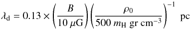 (2)assuming that vA in Eq. (1) is calculated with the total mass density. A theory for the damping of linear MHD waves by ambipolar diffusion was proposed by Balsara (1996), based on a one-dimensional dispersion analysis. He suggested that at large scales, two-fluid MHD turbulence should behave like single-fluid turbulence, while at scales comparable to or smaller than λd, the damping of MHD waves should depend on the Alfvénic Mach number of the flow. More specifically, his theory predicts that the Alfvén and slow magnetosonic waves will be damped when the Alfvén speed is smaller than the sound speed, while if the Alfvén speed is larger than the sound speed, the Alfvén and fast magnetosonic waves will be damped.
Burkhart et al. (2015) confirmed these findings by high-resolution, two-fluid driven MHD turbulence simulations. Using mode decomposition to analyse the different MHD wave modes, they found that sub-Alfvénic turbulence is damped at the ambipolar diffusion scale, while in super-Alvfénic situations the cascade can continue to smaller scales. Our studies include both forced and decaying turbulence with a mean Alfvén speed of about 1.1 km s-1. The decaying turbulence runs start super-Alfvénic and finish sub-Alfvénic, while the driven runs are always sub-Alfvénic. The theory outlined above will be important for the interpretation of our results.
There are many examples of turbulence studies that include ambipolar diffusion. Li et al. (2008) study the statistical behaviour of ideal MHD turbulence and MHD turbulence with ambipolar diffusion, while in a follow-up paper, McKee et al. (2010) study the behaviour of the dense clumps in the same simulations. Their methods, both in the implementation of the ambipolar diffusion and in the analysis of the simulations are different from ours, so the results also differ. We include a detailed comparison with our findings at the end of this paper.
Oishi & Mac Low (2006) simulated supersonic turbulence with ambipolar diffusion and reported the non-appearence of a characteristic scale. However, their study had limited resolution and may not have captured enough of the inertial range. Also, they did not include any explicit calculation of the filament thickness. On the other hand, Downes & O’Sullivan (2011) did observe a significant change in the morphology of their turbulence simulations when they included ambipolar diffusion. Momferratos et al. (2014) studied the properties of diffusive structures created by ambipolar diffusion with a spectral code and found them to be much broader than those created, for example, by Ohmic dissipation. Clearly, there is a dependence on the simulation parameters which needs to be explored further.
The motivation for the present study is to examine whether ion-neutral friction can set a characteristic scale of the filaments created by MHD turbulence. Its aim is not to reproduce the 0.1 pc filament width found in observations, but rather to help understand the physical mechanisms setting this characteristic width. To this end, we perform simulations of MHD turbulence with and without ambipolar diffusion and with careful control of numerical dissipation and compare the sizes and masses of the dense filaments. The numerical method we use for our simulations is explained in Sect. 2 and the main results are described in Sect. 3. The calculations concerning the filament properties are presented in a dedicated section of the paper, Sect. 4. In Sect. 5 we discuss resolution issues. A comparison of our findings with previous work, as well as a discussion of their implications is presented in Sect. 6, while Sect. 7 concludes the paper.
2. Code
We use the publicly available MHD code RAMSES (Teyssier 2002; Fromang et al. 2006) to perform numerical simulations of driven or decaying MHD turbulence. The RAMSES code solves the MHD equations on a Cartesian grid and has adaptive mesh refinement (AMR) capabilities.
The standard version of the code does not include non-ideal MHD terms, so for the purposes of this study we have employed the magnetic diffusion module developed by Masson et al. (2012). The details of the implementation are included in their paper, but we will outline the method here for completeness.
2.1. Ambipolar diffusion implementation
In order to simulate the effects of ambipolar diffusion, the motions of the ions and the neutrals need to be coupled through a friction force Ffr in the momentum equations: 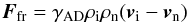 (3)where ρi and ρn are the mass densities of the ions and the neutrals, respectively, while vi and vn are the ion and neutral velocities.
There is more than one possible implementation of this basic principle. One approach is to solve the two-fluid MHD equations and prevent very small timesteps by assuming a low ionization fraction. This implies changing the coupling constant γAD in Eq. (3) accordingly, so this has been called the “heavy ion” approximation (Li et al. 2006; Oishi & Mac Low 2006; Li et al. 2008). Another approach, used by Tilley & Balsara (2008) and Tilley & Balsara (2011), is to implement a semi-implicit scheme. This allows solving the two-fluid equations without having to modify the source terms through Eq. (3).
In this work we are using the so-called “strong coupling” approximation: in a weakly ionized plasma where the collision timescale between ions and neutrals is short compared to the timescales of the problem, the ion pressure and momentum are negligible compared to those of the neutrals. Then the friction force Ffr can be taken roughly equal to the Lorentz force and replaced in the equation of motion of the neutrals, so that one eventually solves one set of MHD equations. Since it requires low ionization conditions, this method is suitable for ambipolar diffusion studies in molecular clouds (Shu et al. 1987; Tóth 1994; Mac Low et al. 1995; Choi et al. 2009).
The equations in the strong coupling limit are: 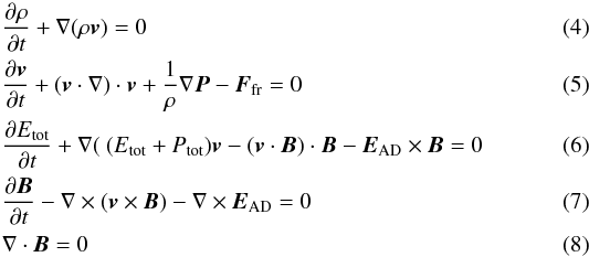 where the additional friction force Ffr has been added to the momentum equation (Eq. (5)) and the electromotive force EAD due to ambipolar diffusion is equal to
 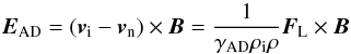 (9)where FL is the Lorenz force.
Like for the calculation of λD in Eq. (2) above, the density of the ions ρi needed in Eq. (3) to calculate the friction force between species is calculated in the code as  , with C = 3 × 10-16 cm−3/2 g1/2. This approximation is only valid for densities higher than roughly 103 cm-3, when ionization happens due to cosmic rays. For lower densities the ionization fraction is approximately constant.
However, in a turbulent environment, underdensities are created in several locations and there might be regions in the simulation domain where the ionization fraction is much higher. This leads to time steps which are pretty small, making the code extremely slow. To tackle this issue the timestep has been limited to a minimum fraction of the Alfvén time by artificially modifying the ionization degree in the regions where the timesteps is smaller than this threshold. A convergence test is presented in the Appendix.
We performed a convergence study for this timestep limit and concluded that below a minimum dt = 0.05ta (where ta the Alfvén crossing time of a cell) the most sensitive results of the simulations (the power spectra) remained unchanged. Although the mass distributions of the filaments and other statistical calculations presented in this work are not greatly affected by the choice of this limit, the simulations we use to draw our final conclusions were integrated with the converged timestep. More details of the ambipolar diffusion module in RAMSES are contained in Masson et al. (2012).
3. MHD simulations
In order to study the effects of ambipolar diffusion on the small-scale structure of turbulence we compare between MHD turbulence simulations with and without the diffusive terms. We simulate both driven and decaying turbulence. None of the simulations includes gravity.
All simulations are performed in three dimensions, in a periodic cubic box of 1 pc size. The average density is 500 cm-3 and the average temperature 10 K, with an isothermal equation of state. The magnetic field is initiated along the z direction with a magnitude of about 15 μG, which gives an initial plasma beta β = 0.1. Given these parameters, we ensure that the mean λd is always well resolved (see Eq. (1) in the Introduction and the discussion later in this section).
Table 1 summarizes the models included in this work. (AD stands for ambipolar diffusion.)
Simulation parameters.
KS comparison.
In the main body of the paper we will present the decaying turbulence results, using runs A0 and B0 as our main reference. The case for driven turbulence is presented in Appendix B.
The turbulent field is created by following the classic recipe from Mac Low et al. (1998), where random phases are given to wave numbers k = 1−4 in Fourier space and amplitudes are chosen to give the desired rms Mach number. We allow the code to iterate for a while until the turbulence has had time to isotropise in the initially uniform density field. All runs are initiated with the same velocity field pattern, multiplied by the appropriate factor to set the desired Mach number or account for energy losses.
The reference runs have an initial Mach number of about 10, decaying to about 3 at the end of the simulation. The driven turbulence runs are kept at a Mach number of 4 by by calculating the difference in kinetic energy with respect to the initial conditions and then adding a static velocity field, multiplied by the appropriate coefficient to account for the energy losses.
3.1. Resolving the physical dissipation length
The challenge we are faced with is to resolve the physical dissipation length while still keeping the size of the problem manageable in terms of computational resources.
The first considerations are to minimize the numerical diffusion and to resolve the inertial range adequately for statistical studies. No matter how great the resolution, in all numerical simulations the smallest scales are affected by numerical viscosity, so one must focus the analysis only on well-resolved structures. The most conservative demand for accurate turbulence studies has been suggested by Federrath et al. (2011), who argue that only scales containing more than 30 cells should be considered resolved. Ideally, we would want all scales down to the ambipolar diffusion length to be resolved with at least 20 cells. However, as we will show, this is not always possible. For reference we have indicated the resolution limit lm (or the associated wavenumber, km) as the length of 20 cells in the power spectra and the thickness histograms throughout the paper.
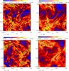 |
Fig. 1 Logarithm of the total gas column density on the yz plane, in cm-2, for the decaying turbulence runs A0 (ideal, left panel) and B0 (ambipolar diffusion, right panel) at t = 5 × 10⁻³ (top) and t = 10-2 (bottom). The black arrows show the projected magnetic field on the same plane. |
Another relevant scale in molecular cloud studies is the sonic length, ls, defined as the length scale at which the rms sonic Mach number of turbulence equals unity (Padoan 1995; McKee et al. 2010). Assuming that the one-dimensional velocity dispersion scales with length like σv ∝ lα, then the sonic Mach number can be written like: 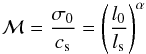 (10)where σ0 the velocity dispersion at the integral scale, l0. We can assume σ0 corresponds to the mean rms sonic Mach number of the turbulence. Then
  (11)For our setup, l0 = 1 pc and, given the Kolmogorov-like behavior of the power spectra (see following sections), α ≃ 1 / 3. Then ls ≃ 0.04 pc for a global rms Mach number of 3, at ls ≃ 0.015 pc for a global rms Mach number of 4 and at ls ≃ 0.008 pc for a global rms Mach number of 5.
An estimate of the mean dissipation length due to ambipolar diffusion in our setup comes from Eq. (1). Using the mean initial values of the experiments, ρ0 = 2 × 10-21 gr cm-3, B = 15 μG, and ρi ≃ 1.3 × 10⁻²⁶ gr cm-3, we calculate a mean dissipation length of about λd ≃ 0.1 pc.
A resolution of 5123 gives a physical grid size of 2 × 10⁻³ pc. Given the values we calculated above, the mean dissipation length is resolved with about 50 cells. Nonetheless, according to Eq. (1), the dissipation length is roughly inversely proportional to the density. This means that at small scales, where the gas is compressed, the dissipation length becomes even smaller. Even if we assume that the magnetic field strength increases in the high-density areas as the square root of the density (Crutcher 2012), which is not strictly true everywhere, a small dependence on the density is left in the expression for the dissipation length.
To study this effect we repeated runs A0 and B0 at a resolution of 10243, although for a shorter time (Runs A0l10 and B0l10 in Table 1). The results of that comparison are presented in Sect. 5.
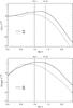 |
Fig. 2 Compensated velocity (top) and log density (bottom) power spectra for runs A0 and B0. Solid lines correspond to run A0 and dashed lines to run B0. The vertical dotted lines show the ambipolar diffusion scale, kAD, calculated for the mean density in the simulation, n0 = 500 cm-3, the resolution scale, km, and the sonic scale, ks. The spectra are shown for a simulation time t = 10-2, which is 0.62 Myr in physical units. The turbulence crossing time is roughly 0.4 Myr. |
3.2. Evolution of the turbulent field
We initialize the simulations with a sonic rms Mach number equal to ℳ = 10 and an Alfvenic Mach number of about  .
.
Figure 1 shows column density contours of the simulation domain on the yz plane, with black arrows indicating the projected magnetic field. The arrow sizes are scaled to the maximum magnitude of the field in the plane. The left panel corresponds to run A0 and the right panel to run B0. Two snapshots are represented in this figure: one at time 5 × 10⁻³ (in code units) at the top, and another at time 10-2 at the bottom. The code time unit corresponds to 62 Myr in physical units, so these correspond to physical times of about 0.3 and 0.6 Myr. The crossing time of the turbulence at Mach 10 is 0.4 Myr, so the second snapshot is at just over one turbulence crossing time.
It is clear that ambipolar diffusion alters the morphology of the density field substantially: Small-scale structure is smoothed out and dense features appear much broader with respect to the ideal MHD run. As the simulation evolves, this effect becomes clearer. The decay is much faster in the non-ideal MHD run and it eliminates small-scale features much more efficiently.
The projected magnetic field topology also changes from one run to another. While at early times A0 and B0 show similar magnetic field configurations, at later times the magnetic field in B0 exhibits a very different behavior. Not only is its magnitude smaller, but at many locations the field lines also have different orientations. This happens due to the loss of both kinetic and magnetic energy through diffusion.
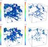 |
Fig. 3 For the last snapshots of runs A0 (top) and B0 (bottom), at code time t = 5 × 10⁻³, volume plots of the logarithm of the mass density above a threshold of 2000 cm-3 (left column) and 5000 cm-3 (right column). |
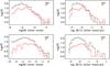 |
Fig. 4 Filament mass (left) and mass per unit length (right) distributions. Black lines show run A0 and red lines run B0. The top panel corresponds to t = 5 × 10⁻³ and the bottom to t = 10-2. The density threshold for defining a filament is 2000 cm-3. |
In order to study the physical processes that cause the broadening of the small-scale structure we can look at the power spectra. The power spectrum of a given quantity v is defined as the mean power of that quantity at each wavenumber k in Fourier space, and is calculated as  . Here
  is the Fourier transform of the quantity v at wave number k. For incompressible MHD turbulence, we expect the power spectrum of the total velocity to have a k− 11 / 3 dependence on the wave number.
When a physical dissipation process such as ambipolar diffusion is modeled in a turbulence simulation, the energy cascade loses power below its scale of influence, which does not depend on resolution. In simulations of ideal MHD turbulence this behavior is mimicked by numerical dissipation, which acts at the scale of a few grid cells, and therefore depends on resolution.
Figure 2 shows the power spectra of the velocity field and the logarithm of the density field, for runs A0 and B0, both divided by the expected k− 11 / 3 dependence. This figure corresponds to the second snapshot (bottom row of Fig. 1), at simulation time t = 10-2. The same spectra for this simulation at time t = 5 × 10⁻³ are included in Fig. 9 of Sect. 5, as well as in Appendix A. The solid lines correspond to run A0 and the dashed lines to run B0.
First, we observe that the inertial range is resolved in all simulations. We also see that the non-ideal simulation exhibits loss of power at small scales, a trend that appears both in the velocity and the log density power spectra. The spectra of the non-ideal MHD run descend steeply above a wave number of about 10. This places the turbulence dissipation scale at around 0.1 pc, in complete agreement with our prediction. In contrast, the ideal MHD run enters the dissipation regime at a smaller scale, roughly at a wave number of 25. This corresponds to about 20 cells, which marks the scales affected by numerical dissipation. Clearly, ion-neutral friction introduces a characteristic dissipation scale, which is likely responsible for the disappearance of small and dense structures.
4. Filament properties
In this section we compare the filaments formed in runs A0 and B0. The process of filament identification and the analysis is the same for all the runs in this paper.
In order to identify filaments in the simulations, we need to have a physical definition of an ISM filament in mind. However, the current definitions for filaments vary in different works. In André et al. (2014) a filament is defined as “any elongated ISM structure with an aspect ratio larger than 5−10 that is significantly overdense with respect to its surroundings”. Könyves et al. (2015) refine this definition to include structures of significant aspect ratios (greater than 3) and column density contrasts of at least 10% with respect to the local background. In the work of Arzoumanian et al. (2011), the Herschel filaments are located by their DisPerSE (Sousbie 2011) skeletons in column density and then their radial density profiles are extracted at different locations along their length to define a thickness. Panopoulou et al. (2014), working with 13CO data (that involves a smaller dynamical range but includes the velocity information), employ a technique similar to that of Arzoumanian et al. (2011) to identify filaments in Taurus.
In this work we define filaments by first setting a density threshold above which a location is considered to belong to a structure of interest. This definition of the structures of interest relates directly to the density-dependent length scale λd from Eq. (2), which facilitates a first interpretation of the results. Direct comparison to the observations requires definitions of the filament and the thickness more similar to the observational ones. Figure 3 shows in logarithm of density the locations remaining once we apply a threshold of 2000 or 5000 cm-3. We will be using these two thresholds throughout this work. Since the mean density of the simulation box is 500 cm-3, these thresholds correspond to density contrasts of 4 and 10, respectively, for all the results included in this paper. The locations above a threshold are then connected into filaments by means of a friend-of-friends algorithm.
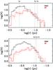 |
Fig. 6 Filament thickness distributions in runs A0 (black lines) and B0 (red lines) at times t = 5 × 10⁻³ (top) and t = 10-2 (bottom). The density threshold for defining a filament is 2000 cm-3. The dotted lines indicate the mean ambipolar diffusion dissipation length λd, calculated from Eq. (1) for this density threshold, the resolution length lm, equal to the length of 20 cells, and the sonic length ls, defined by Eq. (11), for an rms Mach number of 3 (at t = 10-2, bottom) and 5 (at t = 5 × 10⁻³, top). |
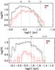 |
Fig. 7 Same as Fig. 6, with a density threshold of 5000 cm-3. The dotted lines indicate the mean ambipolar diffusion dissipation length λd, calculated from Eq. (1) for this density threshold, the resolution length lm, equal to the length of 20 cells, and the sonic length ls, defined by Eq. (11), for an rms Mach number of 3 (at t = 10-2, bottom) and 5 (at t = 5 × 10⁻³, top). |
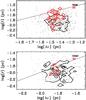 |
Fig. 8 Scatter plots (dots) of the logarithm of the mean filament thickness versus the logarithm of λd in runs A0 (black) and B0 (red). The simulation time is t = 10-2. Shown here are density thresholds 2000 cm-3 (top) and 5000 cm-3 (bottom). The contours show the surface density distribution of the points and the dotted lines show the relation λd = r. |
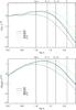 |
Fig. 9 Comparison of the compensated power spectra in different resolutions. At the top, velocity power spectra, and at the bottom, power spectra of the logarithm of the density. As indicated on the label, the solid black line refers to run A0 and the dashed lines refer to runs B0, A0l10 and B0l10. The vertical dotted lines show the mean ambipolar diffusion scale, ⟨ kAD ⟩, the numerical dissipation scales, km,512 and km,1024 of the two resolutions and the sonic scale, ks. Runs A0l10 and B0l10 are run at double spatial resolution compared to A0 and B0. |
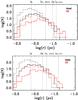 |
Fig. 10 Thickness distributions of runs A0 and B0 at time t = 5 × 10⁻³. Black lines correspond to the ideal MHD runs and red lines to the runs with ambipolar diffusion. The corresponding dashed lines show the 10243 cases. Above, threshold 2000 cm-3 for filament identification, below, threshold of 5000 cm-3. The dotted lines indicate the mean ambipolar diffusion dissipation length λd, calculated from Eq. (1) for each density threshold, the resolution lengths lm,512 and lm,1024, equal to the length of 20 cells, and the sonic length ls, defined by Eq. (11), for an rms Mach number of 5. |
For each filament thus defined we find the eigenvalues of its inertial matrix. The eigenvector associated with the largest of these eigenvalues defines the longest axis of the structure. The filamentary morphology of the structures is clear in Fig. 3, but we have also confirmed it by their aspect ratio distributions, which peak at values larger than 3 for all the simulations.
Each of the three-dimensional filaments is separated into segments along its longest axis and the local center of mass is found for each fragment. The local thickness is calculated by measuring the mass-weighted mean distance of the cells from the local center of mass. Finally, the thickness of the filament is found by taking twice the mean of these measurements over all the segments. This is the same technique used in Hennebelle (2013).
In the following we will compare statistical distributions of the filament properties between ideal and non-ideal MHD runs. In order to quantify the difference between each pair of distributions, we performed a Kolmogorov-Smirnov (KS) two-sample test on each pair of distributions. This test gives the probability that two distributions were drawn from the same sample; in other words, the closer this probability is to zero, the less likely it is that the two distributions were drawn from the same sample (see, for example, Press 1993). KS probability values above about 0.1 indicate that the two distributions are statistically indistinguishable. Table 2 lists the KS probabilities, along with other properties of the distributions.
The mass and mass per unit length distributions of the filaments in runs A0 and B0 are shown in Figs. 4 and 5, for thresholds equal to 2000 cm-3 and 5000 cm-3, respectively. The mass per unit length is calculated as the total mass of a structure divided by the length of its longest axis. The black lines in all these plots refer to ideal MHD and the red lines to runs with ambipolar diffusion.
Looking at the lower density threshold (2000 cm-3) first, we notice that there are clearly fewer low-mass structures when ambipolar diffusion is modeled. In run B0 the peak of the mass distribution shifts to higher values. The distributions evolve slightly with time, but the difference of a factor of 3−10 between the peak masses in the two runs persists. The higher density threshold (5000 cm-3) eliminates many structures in the non-ideal case, confirming the visual impression from Fig. 1. At late times, the statistics are too poor to make any strong statement about the characteristic mass, as indicated by the error bars and by the KS test result in Table 2, but the effect still persists.
The distributions of mass per unit length (right panels of Figs. 4 and 5) greatly resemble the mass distributions. This is not surprising for filamentary structures of similar density. Although with poor statistics, the non-ideal MHD run seems to produce filaments of slightly higher mass per unit length.
The local thicknesses calculated for each center of mass are averaged per structure. Figures 6 and 7 show the distributions of the mean thickness of the identified filaments in runs A0 and B0 for the two different thresholds, 2000 cm-3 and 5000 cm-3, respectively, and for two different times.
From these plots and the corresponding ones for driven turbulence in Appendix B, we recognize a general trend for the ideal MHD simulations to produce a peak in the thickness distribution. This happens because at large scales the turbulence sets a power law, while at scales comparable to the grid size the numerical dissipation gradually removes structure. With ambipolar diffusion this small-scale dependence is less noticeable.
In Fig. 6 we observe that the ion-neutral friction causes the peak of the thickness distribution to move to higher values. The relative shift between the two histograms starts from a factor of 1.6 and at later times evolves to factor of 2.
The statistics with a 5000 cm-3 threshold are again not as good. Even so, we can notice in Fig. 7 that a lot of low-thickness filaments disappear with ambipolar diffusion and in general, the thickness distribution is flatter.
In the Introduction we defined the dissipation length λd. For each dense location in the simulations we calculate λd from Eq. (1) and plot it against the mean thickness of each filament. Figure 8 (and Fig. B.8) show the resulting distributions for the two thresholds, 2000 cm-3 and 5000 cm-3 at the last snapshot of each simulation. Each symbol in these plots corresponds to one filament and the contours show the probability distributions for the same data. Black symbols and lines indicate ideal MHD, red symbols and lines indicate ambipolar diffusion runs. The dotted lines show the relation λd = r. Although strictly speaking there is no definition of λd in the ideal runs, we do plot the quantity expressed by Eq. (1) for comparison.
Although the maximum surface density of points in the non-ideal run falls closer to the λd = r line than the corresponding maximum in the ideal run, there is a tendency in all these diagrams for the measured thickness to be slightly lower than the ambipolar diffusion critical length. This tendency is less pronounced for the higher threshold and for driven turbulence case. We also observe that the distribution of λd values is narrower for the runs with ambipolar diffusion and move to smaller values with higher threshold, in agreement with the theory. The same distributions for the ideal runs spread over a larger range of λd values.
5. Resolution study and convergence
We emphasized before that resolving the physical dissipation regime is essential in this work. But while the power spectra in Fig. 2 (and also Figs. B.2 and B.3) show that the inertial range of turbulence is well resolved with a 5123 grid, numerical diffusion could still be affecting the smallest scales. It is therefore important to study the behavior of the dense structures at higher resolution.
Three additional pairs of runs, ideal and non-ideal MHD, were used to study the effects of numerical diffusion, with the same setup as runs A0 and B0. Two of them were done using AMR with two levels of refinement, two with a lower Courant condition, and two were run entirely on a 10243 grid, without AMR. The clearest effect was shown in this last case, runs A0l10 and B0l10.
These high-resolution simulations are computationally very demanding, especially the cases with ambipolar diffusion. This made long integrations very challenging. We were able to evolve the simulations to a time t = 5 × 10⁻³, the time of the first snapshots in the previous sections.
In Sect. 2 we discussed the need for a timestep limitation in order to stabilize the numerical scheme with the implementation of ambipolar diffusion. We found that the results were converged below a minimum timestep equal to 5 percent of the Alfvén crossing time of the cell. Unfortunately, we were only able to afford a 12.5 percent limit for run B0l10, due to lack of computational resources. Although the mass and thickness distributions are fairly insensitive to the choice of the timestep limit (see Appendix A), the power spectra could still change with a smaller timestep.
The velocity and log density power spectra of runs A0, B0, A0l10 and B0l10 are plotted together in Fig. 9. Despite the obvious expansion of the inertial range with the increase in resolution, the general trend between ideal and non-ideal MHD is unaltered. With ambipolar diffusion the spectra steepen earlier than in the ideal MHD situation. This happens because the physical dissipation length acts on scales larger than those affected by the grid.
Although the difference between runs A0 and A0l10 is marginally higher than that between runs B0 and B0l10, it is evident that the runs have not fully converged in spatial resolution. The power spectra of the non-ideal runs also change when we increase the resolution, extending the inertial range to higher wavenumbers. This either means that the numerical dissipation is affecting also scales we were considering dominated by ambipolar diffusion, or that, even with the ion-neutral friction included, there are modes still capable of transporting power to smaller scales (magnetosonic waves), or both.
The corresponding comparison of the filament thickness distributions between A0, B0, A0l10 and B0l10 is shown in Fig. 10 and it reflects the same picture. The increase in resolution produces much more structure in both cases. The difference between runs A0 and A0l10 is very pronounced, with the peak of the distribution shifting to smaller values by almost 0.5 dex. The peak of the ambipolar diffusion simulations, B0 and B0l10, also shifts, but by a smaller factor, of about 0.3 dex. The largest differences between runs of different resolution are observed towards the smallest values of the filament thickness, in the regime affected by the grid.
Although the relative shift between ideal and non-ideal runs does not change by increasing the resolution, both distributions move to smaller values with respect to their lower resolution counterparts. This is not against our initial expectations. It appears that numerical diffusion still affects the smallest scales. At the same time, the physical dissipation length λd is inversely proportional to the density. Higher resolution allows higher densities to exist in the box, thus the local λd also shrinks. This may indicate that some modes still propagate to smaller scales, an issue we discuss in Sect. 6.
6. Summary and discussion
We have presented high-resolution, ideal and non-ideal MHD simulations of decaying and driven turbulence, with the aim to trace the physics behind the formation of low-density molecular filaments.
The main result of this work is that, in accordance with theoretical predictions, ambipolar diffusion alters the behavior of MHD turbulence. Small-scale structure is smoothed out and the power spectra exhibit clear differences in the extent of the inertial range.
In all these simulations we identified filaments by setting a density threshold and connecting the locations above that threshold with a friends-of-friends algorithm. Then we calculated their masses and thicknesses. We found that both the mass and the thickness distributions of the filaments consistently shift towards higher values with ambipolar diffusion. This result was tested with a Kolmogorov-Smirnov test, which showed that the mass and thickness distributions of the filaments in ideal and non-ideal simulations are genuinely different in most cases, with the exceptions appearing only when the filament statistics are poor.
The parameters used for the turbulent gas in these simulations were chosen to fall close to observed molecular cloud properties, give reasonable range for statistics, but at the same time also allow a very good resolution of the dissipation length for ion-neutral friction, λd, as it is calculated from Eq. (1). Trying to compromise between all these different criteria, with a particular focus on the later, has set a few limitations. The length of the box, for example, is set to 1 pc, which is clearly smaller than most molecular clouds. This choice leads to very small filament masses and masses per unit length , as one can observe in Figs. 4, 5, B.4 and B.5.
In addition, the simulation volume includes several Jeans masses. This makes no difference here because self-gravity is not included, but it would very likely change the picture if it were. Even with these models being in a periodic box with supersonic turbulence we would expect dense regions to collapse rapidly, probably faster than the ambipolar diffusion timescale. On the other hand, self-gravity would also modify the density profiles of some of the filaments, which would allow a more realistic comparison to the observed structures. These matters deserve further investigation, which is outside the scope of this paper. What matters for our present conclusions is the comparison between the ideal and non-ideal MHD situations.
It is instructive to compare our results directly to theories about the dissipation of MHD waves through ambipolar diffusion. Balsara (1996) predicted that, when the Alfvén speed is larger than the sound speed, as it happens in all our simulations, ion-neutral friction damps the Alfvén and fast magnetosonic waves, allowing only the propagation of slow magnetosonic waves. In agreement with this prediction, Burkhart et al. (2015) find that in sub-Alfvénic turbulence the turbulent cascade is completely cut-off below the characteristic ambipolar diffusion scale, while super-Alfvénic turbulence can persist below it.
In this work we have used sub-Alfvénic turbulence for all the models, but the actual situation inside molecular clouds is not known: Padoan & Nordlund (1999) and Lunttila et al. (2009), for example, argue that molecular clouds could be super-Alfvénic, but recent Planck results are more consistent with models of sub-Alfvénic turbulence (Soler et al. 2013; Planck Collaboration Int. XX 2015). Although there is no particular reason for our choice other than our current inability to fully explore the parameter space, a different choice could affect the result.
Our models suggest neither a complete cut-off nor a continuous cascade: on the one hand, the power spectra clearly steepen close to the ambipolar diffusion length λd. (This result is consistent, for example, with the decaying non-ideal turbulence simulations of Momferratos et al. 2014). On the other, we do find structures with thicknesses smaller than the local ambipolar diffusion dissipation length (see, for example, Figs. 8 and B.8). There are two effects that could contribute to this result. One is our filament identification algorithm, which is based on a density threshold. Selecting filaments only above a certain density threshold (roughly equivalent in this study to a density contrast threshold) could be causing a bias towards the densest and thinner part of larger structures. Another is, as Burkhart et al. (2015) argue, that there is a potential dependence of the dissipation scale on the driving scale, which could be the cause of the differences between the freely decaying and the driven runs.
McKee et al. (2010) studied the mass spectra of clumps in non-ideal MHD simulations, varying the so-called ambipolar diffusion Reynolds number, which they define as L/λd (Here L is the integral scale and λd the ambipolar diffusion scale.). They found that, as the ambipolar diffusion Reynolds number decreases, which means ambipolar diffusion becomes stronger, the slope of the higher-mass portion of the clump mass spectrum increases. In our simulations we do not observe such behavior in the high-mass portion of the clump mass function. However, the slope of the intermediate mass regime does seem to change (Figs. 4, 5, B.4 and B.5). Again, it is possible that the source of this apparent discrepancy are the different algorithms for identifying clumps. McKee et al. (2010) use clumpfind, which separates cores in a hierarchical manner. Our algorithm counts everything above a certain density threshold as one structure.
The flattening we observe in the intermediate mass regime of the distributions can be explained if we refer to the density power spectra. Hennebelle & Chabrier (2008) predicted that the exponent of the power law turbulent mass distribution for non-self-gravitating structures should be x = 2−n′/ 3, where n′ is the power spectrum index of log d. The decrease of the power-law slope in the mass spectra with AD is consistent with the change of power-law slope in the log d power spectrum.
Regarding the very important issue of resolution, we dedicated Sect. 5 to the study of convergence of the dissipation length. Although our simulations in principle are resolving the mean characteristic length for ambipolar diffusion, they do not necessarily do so for the densest regions, due to its inverse dependence on the density. We used two simulations with a 10243 resolution, which showed that the runs with ambipolar diffusion are also affected by an increase in resolution. This implies that there are still modes that transport momentum to small scales, in agreement with both Balsara (1996)’s and Burkhart et al. (2015)’s conclusions.
Finally, by increasing the resolution we found that the peak of both the ideal and the non-ideal turbulence distributions shift to lower densities. Whether this is because we have not reached convergence or because the non-ideal thickness distribution also inherently spreads to smaller values is something we could not fully test. In principle, even higher resolution would help resolve this issue, but this is extremely difficult given the current computational resources.
7. Conclusions
The main conclusion of this work is that the introduction of ambipolar diffusion in simulations of supersonic turbulence changes the appearence of the density field and the properties of the densest filaments.
More specifically, we find that the power spectra of both the density and the velocity field show a steeper cutoff, which happens at a smaller wave number in non-ideal MHD than in ideal MHD. This suggests different morphologies and apparent sizes of the dissipative structures with ambipolar diffusion.
The distributions of the filament masses tend to flatten in the high-mass end of the spectrum, which we attribute to the different density scaling.
A very important motivation for this work was the observational finding that the central regions of local molecular filaments as observed in the sub-mm dust continuum with Herschel seem to have a roughly constant thickness of 0.1 pc. As a first step towards understanding the origin of this result, we have sought for any measurable effect of ambipolar diffusion on the distribution of the total width of filaments formed by MHD turbulence. Since our models are limited in dynamical range and do not include dust chemistry or self-gravity, in this attempt we have not used the same definition of the filament width or the same methods as those used in deriving the observational result.
We have defined a filament as a structure of significant overdensity with respect to its surroundings and its width as the mean distance of its points from the local barycenters along its main axis. Using this definition, we find that ambipolar diffusion causes the thickness distributions of the filaments to shift towards higher values. A Kolmogorov-Smirnov test confirms that the differences between almost all pairs of distributions in this paper are statistically highly significant. Moreover, we notice that ambipolar diffusion does not cause a sharp peak around any particular value of the thickness. Due to limitations in spatial dynamical range, we cannot directly compare our findings with, for instance, Herschel observed molecular clouds. Future simulations of larger volumes will allow such comparisons, employing the same tools and adopting the same definitions as those used in analysing observational data.
Finally, we investigated the matter of resolution. Our results show that, although there is clearly a difference between ideal and non-ideal simulations independently of resolution, even the 10243 simulations with ambipolar diffusion are not converged. This is a very important warning for studying the sizes of small-scale structure in numerical simulations of turbulence, especially when no physical dissipation is employed.
Acknowledgments
The authors would like to thank the referee, Mordecai-Mark Mac Low, for very useful discussions and a very constructive report that improved this work and helped put our results better into context. This research has received funding from the European Research Council (FP7/2007-2013 Grant Agreement “ORISTARS” – No. 291294– and Grant Agreement No. 306483).
References
- André, P., Di Francesco, J., Ward-Thompson, D., et al. 2014, Protostars and Planets VI, 27 [Google Scholar]
- André, P., Men’shchikov, A., Bontemps, S., et al. 2010, A&A, 518, L102 [NASA ADS] [CrossRef] [EDP Sciences] [Google Scholar]
- Arzoumanian, D., André, P., Didelon, P., et al. 2011, A&A, 529, L6 [Google Scholar]
- Arzoumanian, D. 2012, Ph.D. Thesis, University Paris 7, France [Google Scholar]
- Balsara, D. S. 1996, ApJ, 465, 775 [NASA ADS] [CrossRef] [Google Scholar]
- Barnard, E. E., Frost, E. B., & Calvert, M. R. 1927, A photographic atlas of selected regions of the Milky Way (Carnegie institution of Washington) [Google Scholar]
- Brandenburg, A., & Zweibel, E. G. 1994, ApJ, 427, L91 [NASA ADS] [CrossRef] [Google Scholar]
- Burkert, A., & Hartmann, L. 2004, ApJ, 616, 288 [NASA ADS] [CrossRef] [Google Scholar]
- Burkhart, B., Lazarian, A., Balsara, D., Meyer, C., & Cho, J. 2015, ApJ, 805, 118 [NASA ADS] [CrossRef] [Google Scholar]
- Choi, E., Kim, J., & Wiita, P. J. 2009, ApJS, 181, 413 [NASA ADS] [CrossRef] [Google Scholar]
- Crutcher, R. M. 2012, ARA&A, 50, 29 [NASA ADS] [CrossRef] [Google Scholar]
- Downes, T. P., & O’Sullivan, S. 2011, ApJ, 730, 12 [NASA ADS] [CrossRef] [Google Scholar]
- Draine, B. T., Roberge, W. G., & Dalgarno, A. 1983, ApJ, 264, 485 [NASA ADS] [CrossRef] [Google Scholar]
- Elmegreen, B. G. 1979, ApJ, 232, 729 [NASA ADS] [CrossRef] [Google Scholar]
- Falgarone, E., & Phillips, T. G. 1990, ApJ, 359, 344 [NASA ADS] [CrossRef] [PubMed] [Google Scholar]
- Federrath, C., Sur, S., Schleicher, D. R. G., Banerjee, R., & Klessen, R. S. 2011, ApJ, 731, 62 [NASA ADS] [CrossRef] [Google Scholar]
- Feitzinger, J. V., & Stuewe, J. A. 1986, ApJ, 305, 534 [NASA ADS] [CrossRef] [Google Scholar]
- Fromang, S., Hennebelle, P., & Teyssier, R. 2006, A&A, 457, 371 [NASA ADS] [CrossRef] [EDP Sciences] [Google Scholar]
- Gómez, G. C., & Vázquez-Semadeni, E. 2014, ApJ, 791, 124 [NASA ADS] [CrossRef] [Google Scholar]
- Heitsch, F. 2013, ApJ, 769, 115 [NASA ADS] [CrossRef] [Google Scholar]
- Heitsch, F., Hartmann, L. W., & Burkert, A. 2008, ApJ, 683, 786 [NASA ADS] [CrossRef] [Google Scholar]
- Heitsch, F., Ballesteros-Paredes, J., & Hartmann, L. 2009, ApJ, 704, 1735 [NASA ADS] [CrossRef] [Google Scholar]
- Hennebelle, P. 2013, A&A, 556, A153 [NASA ADS] [CrossRef] [EDP Sciences] [Google Scholar]
- Hennebelle, P., & André, P. 2013, A&A, 560, A68 [NASA ADS] [CrossRef] [EDP Sciences] [Google Scholar]
- Hennebelle, P., & Chabrier, G. 2008, ApJ, 684, 395 [NASA ADS] [CrossRef] [Google Scholar]
- Hennebelle, P., Banerjee, R., Vázquez-Semadeni, E., Klessen, R. S., & Audit, E. 2008, A&A, 486, L43 [NASA ADS] [CrossRef] [EDP Sciences] [Google Scholar]
- Kim, W.-T., Ostriker, E. C., & Stone, J. M. 2003, ApJ, 599, 1157 [NASA ADS] [CrossRef] [Google Scholar]
- Könyves, V., André, P., Men’shchikov, A., et al. 2015, A&A, 584, A91 [NASA ADS] [CrossRef] [EDP Sciences] [Google Scholar]
- Kulsrud, R., & Pearce, W. P. 1969, ApJ, 156, 445 [NASA ADS] [CrossRef] [Google Scholar]
- Larson, R. B. 1981, MNRAS, 194, 809 [NASA ADS] [CrossRef] [Google Scholar]
- Li, H.-b., & Houde, M. 2008, ApJ, 677, 1151 [NASA ADS] [CrossRef] [Google Scholar]
- Li, P. S., McKee, C. F., & Klein, R. I. 2006, ApJ, 653, 1280 [Google Scholar]
- Li, P. S., McKee, C. F., Klein, R. I., & Fisher, R. T. 2008, ApJ, 684, 380 [NASA ADS] [CrossRef] [Google Scholar]
- Lunttila, T., Padoan, P., Juvela, M., & Nordlund, Å. 2009, ApJ, 702, L37 [NASA ADS] [CrossRef] [Google Scholar]
- Mac Low, M.-M., Norman, M. L., Königl, A., & Wardle, M. 1995, ApJ, 442, 726 [NASA ADS] [CrossRef] [Google Scholar]
- Mac Low, M.-M., Smith, M. D., Klessen, R. S., & Burkert, A. 1998, Ap&SS, 261, 195 [NASA ADS] [CrossRef] [Google Scholar]
- Masson, J., Teyssier, R., Mulet-Marquis, C., Hennebelle, P., & Chabrier, G. 2012, ApJS, 201, 24 [NASA ADS] [CrossRef] [Google Scholar]
- McKee, C. F., Li, P. S., & Klein, R. I. 2010, ApJ, 720, 1612 [NASA ADS] [CrossRef] [Google Scholar]
- Moeckel, N., & Burkert, A. 2015, ApJ, 807, 67 [NASA ADS] [CrossRef] [Google Scholar]
- Molinari, S., Swinyard, B., Bally, J., et al. 2010, A&A, 518, L100 [NASA ADS] [CrossRef] [EDP Sciences] [Google Scholar]
- Momferratos, G., Lesaffre, P., Falgarone, E., & Pineau des Forêts, G. 2014, MNRAS, 443, 86 [NASA ADS] [CrossRef] [Google Scholar]
- Mouschovias, T. C. 1991, ApJ, 373, 169 [NASA ADS] [CrossRef] [Google Scholar]
- Myers, P. C. 2009, ApJ, 700, 1609 [NASA ADS] [CrossRef] [EDP Sciences] [Google Scholar]
- Ntormousi, E., Burkert, A., Fierlinger, K., & Heitsch, F. 2011, ApJ, 731, 13 [NASA ADS] [CrossRef] [Google Scholar]
- Oishi, J. S., & Mac Low, M.-M. 2006, ApJ, 638, 281 [NASA ADS] [CrossRef] [Google Scholar]
- Padoan, P. 1995, MNRAS, 277, 377 [NASA ADS] [CrossRef] [Google Scholar]
- Padoan, P., & Nordlund, Å. 1999, ApJ, 526, 279 [NASA ADS] [CrossRef] [Google Scholar]
- Padoan, P., Jimenez, R., Nordlund, Å., & Boldyrev, S. 2004, Phys. Rev. Lett., 92, 191102 [NASA ADS] [CrossRef] [PubMed] [Google Scholar]
- Palmeirim, P., André, P., Kirk, J., et al. 2013, A&A, 550, A38 [NASA ADS] [CrossRef] [EDP Sciences] [Google Scholar]
- Panopoulou, G. V., Tassis, K., Goldsmith, P. F., & Heyer, M. H. 2014, MNRAS, 444, 2507 [NASA ADS] [CrossRef] [Google Scholar]
- Planck Collaboration Int. XX. 2015, A&A, 576, A105 [NASA ADS] [CrossRef] [EDP Sciences] [Google Scholar]
- Press, W. H. 1993, Science, 259, 1931 [NASA ADS] [Google Scholar]
- Schisano, E., Rygl, K. L. J., Molinari, S., et al. 2014, ApJ, 791, 27 [NASA ADS] [CrossRef] [Google Scholar]
- Schneider, S., & Elmegreen, B. G. 1979, ApJS, 41, 87 [NASA ADS] [CrossRef] [Google Scholar]
- Shu, F. H., Lizano, S., & Adams, F. C. 1987, in Star Forming Regions, eds. M. Peimbert, & J. Jugaku, IAU Symp., 115, 417 [Google Scholar]
- Smith, R. J., Glover, S. C. O., Clark, P. C., Klessen, R. S., & Springel, V. 2014, MNRAS, 441, 1628 [NASA ADS] [CrossRef] [Google Scholar]
- Soler, J. D., Hennebelle, P., Martin, P. G., et al. 2013, ApJ, 774, 128 [NASA ADS] [CrossRef] [Google Scholar]
- Sousbie, T. 2011, MNRAS, 414, 350 [NASA ADS] [CrossRef] [Google Scholar]
- Tassis, K., & Mouschovias, T. C. 2004, ApJ, 616, 283 [NASA ADS] [CrossRef] [Google Scholar]
- Teyssier, R. 2002, A&A, 385, 337 [NASA ADS] [CrossRef] [EDP Sciences] [Google Scholar]
- Tilley, D. A., & Balsara, D. S. 2008, MNRAS, 389, 1058 [NASA ADS] [CrossRef] [Google Scholar]
- Tilley, D. A., & Balsara, D. S. 2011, MNRAS, 415, 3681 [NASA ADS] [CrossRef] [Google Scholar]
- Tóth, G. 1994, ApJ, 425, 171 [NASA ADS] [CrossRef] [Google Scholar]
- Williams, J. P., Blitz, L., & McKee, C. F. 2000, Protostars and Planets IV, 97 [Google Scholar]
- Zweibel, E. G., & Josafatsson, K. 1983, ApJ, 270, 511 [CrossRef] [Google Scholar]
Appendix A: Timestep convergence
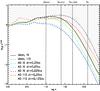 |
Fig. A.1 Compensated velocity power spectra for decaying turbulence simulations at time t = 5 × 10⁻³ using different timestep limits. The black solid line corresponds to the ideal 5123 run and the black dashed line to the ideal 10243 run. The vertical dotted lines show the mean ambipolar diffusion scale, ⟨ kAD ⟩, the numerical dissipation scales, km,512 and km,1024 of the two resolutions and the sonic scale, ks (ks and km,1024 are practically the same). Run B0, used as reference in the main body of the paper, uses a timestep limit dt = 0.05ta, where ta the Alfvén crossing time of a cell. |
In Sect. 2 we mentioned the necessary timestep limitation as part of the non-ideal MHD implementation we used for this work. Although this limitation stabilizes the numerical scheme, it can also affect the accuracy of the result. Here we include some results of a convergence study on this timestep limit which led to the adopted dt = 0.05ta (where ta the Alfvén crossing time of a cell) in the reference run B0.
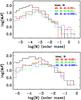 |
Fig. A.2 Mass distributions for decaying turbulence simulations at time t = 5 × 10⁻³ using different timestep limits. The black solid line corresponds to the ideal 5123 run and the colored lines to runs with ambipolar diffusion and different timestep limits. ta is the Alfvén crossing time of a cell. Top: density threshold of 2000 cm-3, bottom: 5000 cm-3. |
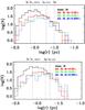 |
Fig. A.3 Filament thickness distributions for decaying turbulence simulations at time t = 5 × 10⁻³ using different timestep limits. The black solid line corresponds to the ideal 5123 run and the colored lines to runs with ambipolar diffusion and different timestep limits. ta is the Alfvén crossing time of a cell. Top: density threshold of 2000 cm-3, bottom: 5000 cm-3. The dotted lines indicate the mean ambipolar diffusion dissipation length λd, calculated from Eq. (1) for each density threshold, the resolution lengths lm,512 and lm,1024, equal to the length of 20 cells, and the sonic length ls, defined by Eq. (11), for an rms Mach number of 5. |
Figure A.1 shows power spectra of decaying turbulence models with decreasing timestep limits for the ambipolar diffusion scheme. Figures A.2 and A.3 show the filament mass and thickness distributions for the same models, like in Sect. 4 of this paper.
Not surprisingly, the velocity power spectra seem to be much more sensitive to the change of timestep limit than the mass and thickness distributions. The velocities are a direct output of the code, while the mass and thickness distributions are derived quantities. It is clear that allowing timesteps smaller than dt = 0.05ta does not affect the power spectra, so we have adopted this limit for the reference run.
Since the mass and thickness distributions seem to be insensitive to the timestep limit, we do include some results of the high resolution run B0l10 in this paper, however keeping these small uncertainties in mind.
Appendix B: Driven turbulence
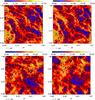 |
Fig. B.1 Logarithm of the total gas column density on the xy plane, in cm-2, for driven turbulence runs A1 (ideal, left panel) and B1 (ambipolar diffusion, right panel) at t = 5 × 10⁻³ (top) and t = 10-2 (bottom). The black arrows show the projected magnetic field on the same plane. |
Turbulence in an ideal MHD simulation decays through numerical resistivity, existent in all numerical codes. When a physical diffusive process is explicitly modeled, there can be some doubts on whether or not it behaves as a scaled-up version of the numerical resistivity, causing the same effect at a faster rate, or if it qualitatively alters the behavior of the simulation. If the former is true, one would expect the ideal MHD run to eventually reach a state of the AD run at a later time.
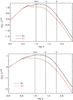 |
Fig. B.2 Compensated velocity power spectra for runs A1 and B1. Red lines correspond to run A0 and blue lines to run B0. The spectra are shown for two simulation times: at the top, t = 5 × 10⁻³ and at the bottom, t = 10-2. The vertical dotted lines show the mean ambipolar diffusion scale, ⟨ kAD ⟩, the numerical dissipation scales, km and the sonic scale, ks. |
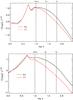 |
Fig. B.3 Compensated power spectra of the logarithm of the density at t = 5 × 10⁻³ (left) and t = 10-2 (right). Red lines correspond to run A1 and blue lines to run B1. |
In order to investigate this, we performed two numerical experiments of forced turbulence. In these simulations, turbulent kinetic energy is replenished at each coarse time step by the same amount that was dissipated in the last timestep.
Figure B.1 shows the logarithm of the column density for runs A1 and B1, overplotted with black arrows to illustrate the projected magnetic field. The snapshots were taken at the same simulation times as the ones in Fig. 1 for the decaying run.
Although less pronounced, the disappearance of small-scale features and the relative lack of dense regions that we observed between runs A0 and B0 are still evident in run B1 with respect to run A1. However, contrary to the decaying turbulence situation, in this case the projected magnetic field maintains a very similar morphology between ideal and non-ideal runs. This probably happens because we keep adding velocities with the same spatial configuration, so the magnetic field is also constantly re-created.
Figures B.2 and B.3 show the power spectra of the velocity and of the logarithm of the density. The inertial range is clearly smaller in comparison to runs A0 and B0. Distinctive peaks appear in both the density and the velocity power spectra, corresponding to the driving scales. In addition, the ambipolar diffusion scale is larger here compared to the decaying runs, which also contributes to the loss of scales in the inertial range.
Nonetheless, the non-ideal run shows less power in small scales both in density and in velocity, which is the same trend we observed in the case of decaying turbulence. This is clear evidence that ambipolar diffusion dominates over numerical dissipation in our simulations.
Appendix B.1: Filament properties
Figures B.4 and B.5 show the mass and mass per unit length distributions of the filaments in runs A1 and B1. The shift of the peak mass to higher values with ambipolar diffusion is also observed here, but it is much clearer at later times.
The same trend appears in the distributions of the mean filament thickness, shown in Figs. B.6 and B.7. While at early times the distributions appear similar, as time advances they separate by a factor of 1.8.
Figure B.8 shows the relative distributions of critical length and filament thickness, like Fig. 8 in Sect. 4. The picture is the same as the one we described for the decaying turbulence situation: the thickness of the filaments we measure agrees very well with the estimate of the local critical length for ambipolar diffusion, with the critical length being much better defined in the non-ideal simulations.
Overall, runs A1 and B1, although at a different Mach number and with turbulence constantly driven, point to the same result as the decaying turbulence runs A0 and B0, that ambipolar diffusion cuts the turbulent cascade off at a larger scale, creating on average dense structures of larger thickness.
 |
Fig. B.4 Filament mass (left) and mass per unit length (right) distributions. Black lines show run A1 and red lines run B1. The top panel corresponds to t = 5 × 10⁻³ and the bottom to t = 10-2. The density threshold for defining a filament is 2000 cm-3. |
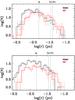 |
Fig. B.6 Filament thickness distributions in runs A1 (black lines) and B1 (red lines) at times t = 5 × 10⁻³ (top) and t = 10-2 (bottom). The density threshold for defining a filament is 2000 cm-3. The dotted lines indicate the mean ambipolar diffusion dissipation length λd, calculated from Eq. (1) for this density threshold, the resolution length lm, equal to the length of 20 cells, and the sonic length ls, defined by Eq. (11), for an rms Mach number of 4. |
All Tables
All Figures
|
Fig. 1 Logarithm of the total gas column density on the yz plane, in cm-2, for the decaying turbulence runs A0 (ideal, left panel) and B0 (ambipolar diffusion, right panel) at t = 5 × 10⁻³ (top) and t = 10-2 (bottom). The black arrows show the projected magnetic field on the same plane. |
| In the text | |
|
Fig. 2 Compensated velocity (top) and log density (bottom) power spectra for runs A0 and B0. Solid lines correspond to run A0 and dashed lines to run B0. The vertical dotted lines show the ambipolar diffusion scale, kAD, calculated for the mean density in the simulation, n0 = 500 cm-3, the resolution scale, km, and the sonic scale, ks. The spectra are shown for a simulation time t = 10-2, which is 0.62 Myr in physical units. The turbulence crossing time is roughly 0.4 Myr. |
| In the text | |
|
Fig. 3 For the last snapshots of runs A0 (top) and B0 (bottom), at code time t = 5 × 10⁻³, volume plots of the logarithm of the mass density above a threshold of 2000 cm-3 (left column) and 5000 cm-3 (right column). |
| In the text | |
|
Fig. 4 Filament mass (left) and mass per unit length (right) distributions. Black lines show run A0 and red lines run B0. The top panel corresponds to t = 5 × 10⁻³ and the bottom to t = 10-2. The density threshold for defining a filament is 2000 cm-3. |
| In the text | |
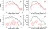 |
Fig. 5 Same as Fig. 4, for a density threshold of 5000 cm-3. |
| In the text | |
|
Fig. 6 Filament thickness distributions in runs A0 (black lines) and B0 (red lines) at times t = 5 × 10⁻³ (top) and t = 10-2 (bottom). The density threshold for defining a filament is 2000 cm-3. The dotted lines indicate the mean ambipolar diffusion dissipation length λd, calculated from Eq. (1) for this density threshold, the resolution length lm, equal to the length of 20 cells, and the sonic length ls, defined by Eq. (11), for an rms Mach number of 3 (at t = 10-2, bottom) and 5 (at t = 5 × 10⁻³, top). |
| In the text | |
|
Fig. 7 Same as Fig. 6, with a density threshold of 5000 cm-3. The dotted lines indicate the mean ambipolar diffusion dissipation length λd, calculated from Eq. (1) for this density threshold, the resolution length lm, equal to the length of 20 cells, and the sonic length ls, defined by Eq. (11), for an rms Mach number of 3 (at t = 10-2, bottom) and 5 (at t = 5 × 10⁻³, top). |
| In the text | |
|
Fig. 8 Scatter plots (dots) of the logarithm of the mean filament thickness versus the logarithm of λd in runs A0 (black) and B0 (red). The simulation time is t = 10-2. Shown here are density thresholds 2000 cm-3 (top) and 5000 cm-3 (bottom). The contours show the surface density distribution of the points and the dotted lines show the relation λd = r. |
| In the text | |
|
Fig. 9 Comparison of the compensated power spectra in different resolutions. At the top, velocity power spectra, and at the bottom, power spectra of the logarithm of the density. As indicated on the label, the solid black line refers to run A0 and the dashed lines refer to runs B0, A0l10 and B0l10. The vertical dotted lines show the mean ambipolar diffusion scale, ⟨ kAD ⟩, the numerical dissipation scales, km,512 and km,1024 of the two resolutions and the sonic scale, ks. Runs A0l10 and B0l10 are run at double spatial resolution compared to A0 and B0. |
| In the text | |
|
Fig. 10 Thickness distributions of runs A0 and B0 at time t = 5 × 10⁻³. Black lines correspond to the ideal MHD runs and red lines to the runs with ambipolar diffusion. The corresponding dashed lines show the 10243 cases. Above, threshold 2000 cm-3 for filament identification, below, threshold of 5000 cm-3. The dotted lines indicate the mean ambipolar diffusion dissipation length λd, calculated from Eq. (1) for each density threshold, the resolution lengths lm,512 and lm,1024, equal to the length of 20 cells, and the sonic length ls, defined by Eq. (11), for an rms Mach number of 5. |
| In the text | |
|
Fig. A.1 Compensated velocity power spectra for decaying turbulence simulations at time t = 5 × 10⁻³ using different timestep limits. The black solid line corresponds to the ideal 5123 run and the black dashed line to the ideal 10243 run. The vertical dotted lines show the mean ambipolar diffusion scale, ⟨ kAD ⟩, the numerical dissipation scales, km,512 and km,1024 of the two resolutions and the sonic scale, ks (ks and km,1024 are practically the same). Run B0, used as reference in the main body of the paper, uses a timestep limit dt = 0.05ta, where ta the Alfvén crossing time of a cell. |
| In the text | |
|
Fig. A.2 Mass distributions for decaying turbulence simulations at time t = 5 × 10⁻³ using different timestep limits. The black solid line corresponds to the ideal 5123 run and the colored lines to runs with ambipolar diffusion and different timestep limits. ta is the Alfvén crossing time of a cell. Top: density threshold of 2000 cm-3, bottom: 5000 cm-3. |
| In the text | |
|
Fig. A.3 Filament thickness distributions for decaying turbulence simulations at time t = 5 × 10⁻³ using different timestep limits. The black solid line corresponds to the ideal 5123 run and the colored lines to runs with ambipolar diffusion and different timestep limits. ta is the Alfvén crossing time of a cell. Top: density threshold of 2000 cm-3, bottom: 5000 cm-3. The dotted lines indicate the mean ambipolar diffusion dissipation length λd, calculated from Eq. (1) for each density threshold, the resolution lengths lm,512 and lm,1024, equal to the length of 20 cells, and the sonic length ls, defined by Eq. (11), for an rms Mach number of 5. |
| In the text | |
|
Fig. B.1 Logarithm of the total gas column density on the xy plane, in cm-2, for driven turbulence runs A1 (ideal, left panel) and B1 (ambipolar diffusion, right panel) at t = 5 × 10⁻³ (top) and t = 10-2 (bottom). The black arrows show the projected magnetic field on the same plane. |
| In the text | |
|
Fig. B.2 Compensated velocity power spectra for runs A1 and B1. Red lines correspond to run A0 and blue lines to run B0. The spectra are shown for two simulation times: at the top, t = 5 × 10⁻³ and at the bottom, t = 10-2. The vertical dotted lines show the mean ambipolar diffusion scale, ⟨ kAD ⟩, the numerical dissipation scales, km and the sonic scale, ks. |
| In the text | |
|
Fig. B.3 Compensated power spectra of the logarithm of the density at t = 5 × 10⁻³ (left) and t = 10-2 (right). Red lines correspond to run A1 and blue lines to run B1. |
| In the text | |
|
Fig. B.4 Filament mass (left) and mass per unit length (right) distributions. Black lines show run A1 and red lines run B1. The top panel corresponds to t = 5 × 10⁻³ and the bottom to t = 10-2. The density threshold for defining a filament is 2000 cm-3. |
| In the text | |
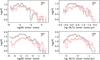 |
Fig. B.5 Same as Fig. B.4, for a density threshold equal to 5000 cm-3. |
| In the text | |
|
Fig. B.6 Filament thickness distributions in runs A1 (black lines) and B1 (red lines) at times t = 5 × 10⁻³ (top) and t = 10-2 (bottom). The density threshold for defining a filament is 2000 cm-3. The dotted lines indicate the mean ambipolar diffusion dissipation length λd, calculated from Eq. (1) for this density threshold, the resolution length lm, equal to the length of 20 cells, and the sonic length ls, defined by Eq. (11), for an rms Mach number of 4. |
| In the text | |
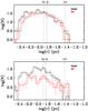 |
Fig. B.7 Same as Fig. B.6, with a density threshold of 5000 cm-3. |
| In the text | |
 |
Fig. B.8 Same as Fig. 8, for runs A1 (black) and B1 (red). |
| In the text | |
Current usage metrics show cumulative count of Article Views (full-text article views including HTML views, PDF and ePub downloads, according to the available data) and Abstracts Views on Vision4Press platform.
Data correspond to usage on the plateform after 2015. The current usage metrics is available 48-96 hours after online publication and is updated daily on week days.
Initial download of the metrics may take a while.