| Issue |
A&A
Volume 588, April 2016
|
|
|---|---|---|
| Article Number | A91 | |
| Number of page(s) | 15 | |
| Section | Extragalactic astronomy | |
| DOI | https://doi.org/10.1051/0004-6361/201527799 | |
| Published online | 23 March 2016 | |
Metallicity gradients in local Universe galaxies: Time evolution and effects of radial migration
1
INAF–Osservatorio Astrofisico di Arcetri, Largo E. Fermi, 5
50125
Firenze,
Italy
e-mail:
This email address is being protected from spambots. You need JavaScript enabled to view it.
2
ESO Karl-Schwarzchild str., 2, 85748
Garching b. Munchen,
Germany
3
National Optical Astronomy Observatory,
950 N. Cherry Avenue,
Tucson, AZ
85719,
USA
Received: 20 November 2015
Accepted: 7 February 2016
Abstract
Context. Our knowledge of the shape of radial metallicity gradients in disc galaxies has recently improved. Conversely, the understanding of their time evolution is more complex, since it requires analysis of stellar populations with different ages or systematic studies of galaxies at different redshifts. In the local Universe, H ii regions and planetary nebulae (PNe) are important tools to investigate radial metallicity gradients in disc galaxies.
Aims. We present an in-depth study of all nearby spiral galaxies (M33, M31, NGC 300, and M81) with direct-method nebular abundances of both populations, aiming at studying the evolution of their radial metallicity gradients. For the first time, we also evaluate the radial migration of PN populations.
Methods. For the selected galaxies, we analysed H ii region and PN properties to: determine whether oxygen in PNe is a reliable tracer for past interstellar medium (ISM) composition; homogenise published datasets; estimate the migration of the oldest stellar populations; and determine the overall chemical enrichment and slope evolution.
Results. We confirm that oxygen in PNe is a reliable tracer for past ISM metallicity. We find that PN gradients are flatter than or equal to those of H ii regions. When radial motions are negligible, this result provides a direct measurement of the time evolution of the gradient. For galaxies with dominant radial motions, we provide upper limits on the gradient evolution. Finally, the total metal content increases with time in all target galaxies, and early morphological types have a larger increment Δ(O/H) than late-type galaxies.
Conclusions. Our findings provide important constraints to discriminate among different galactic evolutionary scenarios, favouring cosmological models with enhanced feedback from supernovae. The advent of extremely large telescopes allows us to include galaxies in a wider range of morphologies and environments, thus putting firmer constraints on galaxy formation and evolution scenarios.
Key words: ISM: abundances / Hii regions / planetary nebulae: general / galaxies: abundances / galaxies: evolution / Local Group
© ESO, 2016
1. Introduction
Spiral galaxies are complex astrophysical objects that manifest a non-uniform distribution of metals across their discs. Their radial metallicity distribution, known as the radial metallicity gradient, has been studied for a long time, starting with the pioneering works by Aller (1942) and later by Searle (1971) and Pagel & Edmunds (1981). In recent years, the existence of radial metallicity gradients in spiral galaxies has been tackled in the following cases: individual nearby galaxies, for which direct-method measurements are available, i.e. abundance analysis that involves the measurement of electron temperature and density diagnostic emission lines to characterise the physical conditions of the plasma (see e.g. Bresolin 2007; Bresolin et al. 2009; Berg et al. 2012, 2013, 2015); large samples of intermediate distance galaxies, where H ii region abundances are derived from the detection of several “strong” emission lines (see e.g. Sánchez et al. 2014); and high-redshift galaxies (see e.g. Cresci et al. 2010; Jones et al. 2010, 2013, 2015).
In our Galaxy, metallicity gradients have been estimated using several tracers, from those of relatively young ages, such as OB stars (e.g. Daflon & Cunha 2004), Cepheids (e.g. Andrievsky et al. 2004; Luck et al. 2006; Yong et al. 2006), H ii regions (e.g. Deharveng et al. 2000; Esteban et al. 2005; Rudolph et al. 2006; Balser et al. 2011), to those of intermediate-to-old ages, such as planetary nebulae (PNe; e.g. Maciel et al. 2003; Henry et al. 2010; Stanghellini & Haywood 2010), and open clusters (e.g. Friel 1995; Chen et al. 2003; Magrini et al. 2009a).
The general result is that most spiral galaxies show negative radial gradients within their optical radius. In addition, when the observations are deep enough to investigate the outskirts of galaxies, it has been often found that the metallicity tends to reach a plateau: in external galaxies whose gradients are marked by H ii regions (Bresolin et al. 2009, 2012; Goddard et al. 2011; Werk et al. 2011) and in our own Galaxy using open clusters (Sestito et al. 2006; Magrini et al. 2009a; Lépine et al. 2011), H ii regions (Vilchez & Esteban 1996), and PNe (Maciel & Quireza 1999)1.
If we focus on regions within the galactic optical radius, where the gradients are clearly negative, the most important open questions are: How was the present time radial gradient established? Was it steeper or flatter in the past? Finding answers to these questions has important implications to our understanding of the processes that lead to disc formation. In particular, observations allow us to put strong constraints on galactic formation and evolution models (e.g. Pilkington et al. 2012a,b; Gibson et al. 2013; Stinson et al. 2013).
In classical chemical evolution models in which the cosmological context and gas and star dynamics are neglected, different predictions on the time evolution of radial metallicity gradients depend on the pre-enrichment of the material that formed the primordial disc and whether one assumes a gas density threshold for star formation. A disc formed by pre-enriched gas, and in which a minimum gas density is required to permit the formation of new stars, naturally develops an initial flat metallicity gradient that becomes steeper with time (see e.g. Chiappini et al. 2001). On the other hand, in models in which the disc is formed by primordial gas and the star formation can proceed at any gas density, the radial metallicity gradient is typically steeper at early times and flattens as the galaxy evolves (Ferrini et al. 1994; Hou et al. 2000; Mollá & Díaz 2005; Magrini et al. 2009a). Recently, Gibson et al. (2013) have examined the role of energy feedback in shaping the time evolution of abundance gradients within a subset of cosmological hydrodynamical disc simulations drawn from the MUGS (McMaster Unbiased Galaxy Simulations; Stinson et al. 2010) and MaGICC (Making Galaxies in a Cosmological Context; Brook et al. 2012) samples. The two sets of simulations adopt two feedback schemes: the conventional one in which about 10−40% of the energy associated with each supernova (SN) is used to heat the interstellar medium (ISM) and the enhanced feedback model in which a larger quantity of energy per SN is released, distributed, and recycled over large scales. The resulting time evolution of the radial gradients is different in the two cases: a strong flattening with time in the former and a relatively flat and temporally invariant abundance gradients in the latter.
In addition, the modelling of the chemical evolution of the galactic disc needs to be combined with dynamics. Both observations and numerical simulations show that stars move from their birth places and migrate throughout the disc during their lifetimes. In our Galaxy, the age-metallicity relationship in the solar neighbourhood puts strong constraints on the presence of radial migration (Edvardsson et al. 1993; Haywood 2008; Schönrich & Binney 2009; Minchev & Famaey 2010). For any given age, there are stars in the solar neighbourhood with a wide range of metallicities and this can only explained with an exceptionally inhomogeneous ISM or, more likely, with radial migration. From a theoretical point of view, radial stellar migration is related to several processes such as the presence of transient spirals (Sellwood & Binney 2002; Roškar et al. 2008), mergers and perturbations from satellite galaxies and sub-haloes that can induce radial mixing (Quillen et al. 2009), and a central bar that can stimulate a strong exchange of angular momentum when associated with a spiral structure (Minchev & Famaey 2010; Minchev et al. 2011; Di Matteo et al. 2013; Kubryk et al. 2013). Minchev et al. (2014), by separating the effects of kinematic heating and radial migration, showed the importance of migration that is needed to explain the oldest and hottest stellar population, especially. Finally, recent analysis of the SDSS-III/Apache Point Observatory Galactic Evolution Experiment (APOGEE) data has revealed that the Galactic metallicity distribution function changes shape as a function of radius. Loebman et al. (2016) explained this effect in terms of radial migration, in particular, as a result of metal-rich stars that formed in the inner disc and subsequently migrated towards the metal-poorer outer disc.
From an observational point of view, the time evolution of the radial metallicity gradient in nearby external galaxies is well studied with two tracers with similar spectroscopic features, characterising to two different epochs in a galaxy lifetime: H ii regions and PNe. Studies of PNe and H ii region gradients from direct-method abundances in M33 (Magrini et al. 2009b, 2010; Bresolin et al. 2010), M81 (Stanghellini et al. 2010, 2014), NGC 300 (Bresolin et al. 2009; Stasińska et al. 2013), and M31 (Zurita & Bresolin 2012) have produced a limited array of results, all indicating gradient invariance or steepening of the radial O/H gradient with time. These results, summarised in Fig. 9 of Stanghellini et al. (2014), need to be validated by a thorough and homogeneous analysis of all the available data and the gradients need to be recalculated over a common galactocentric scale for all sample galaxies.
The paper is organised as follows: in Sect. 2 we prove the reliability of PN abundances to investigate the past ISM composition through the invariance of O (at first order) during the lifetime of PN progenitors, while in Sect. 3 we present our sample of spiral galaxies with the observational datasets. In Sect. 4 we estimate the effects of radial migration in M31 and M33. In Sect. 5 we describe the adopted method to homogenise the literature data and to study the time-evolution of radial metallicity gradients. In Sect. 6 we summarise our results and in Sect. 7 we discuss them. We give our summary and conclusions in Sect. 8.
2. Tracing the past: the composition of interstellar medium
H ii regions are among the best tracers of the present-time composition of ISM since these regions are ionised by young massive OB stars that did not have enough time to move from their birth place. On the other hand, PNe are the gaseous remnants of relatively old stellar populations. Before using them as tracers of past ISM composition, we must consider the nucleosynthesis and mixing processes taking place during their evolution that could modify their composition, and the relevance of their dynamics that could displace them from their initial place of birth (see Sect. 4).
To obtain a reliable determination of the chemical composition of a nebula from emission lines, we need accurate measurements of the nebula’s physical properties, such as electron temperature Te and density Ne. Elemental abundances are often derived from the measurement of collisionally excited lines (CELs), which are very sensitive to Te. The electron temperature is derived from the CEL ratios, such as [Oiii] λ4363/(λ4959 + λ5007) and [Nii] λ 5755/(λ6548 + λ6584) nebular-to-auroral line ratios (Osterbrock & Ferland 2006).
An alternative method for nebular abundance determinations is to use the ratio of the intensity of an optical recombination line (ORL) of He or a heavy element, such as O or N, with that of H. The ORLs are less affected by temperature measurement errors since they have a weak dependence on Te and Ne. In regions where both CEL and ORL abundances are available, the ORLs give systematically higher abundances than CELs (e.g. Peimbert et al. 1993; Liu et al. 1995, 2001; Tsamis et al. 2004; García-Rojas & Esteban 2007). This behaviour has been explained, for instance, with the bi-abundance nebular model by Liu et al. (2000) in which the ORLs abundances arise from cold H-deficient small portions of the nebulae, while the strong CELs are emitted predominantly from the warmer ionised gas, and thus are more representative of the global nebular abundance. In addition, ORLs are much weaker than CELs and, consequently, they can be used to measure abundances in nearby or bright sources only. Thus, in most extragalactic studies, CELs are adopted to trace the chemical composition and the total abundance of a given element is computed by summing the abundances of different ionisation stages of that element.
However, not all ions are observable in the optical range, and since almost all abundance measurements are based on optical spectroscopy, the ionic sum may underestimate the atomic abundances. The contribution of the unseen ions is usually estimated introducing the so-called ionisation correction factors (ICFs), often based on photoionisation models (Kingsburgh & Barlow 1994; Kwitter & Henry 2001; Delgado-Inglada et al. 2014). In this framework, O is the best measured element in PNe (and H ii regions) because (i) we can directly measure its electron temperatures Te([Oiii]) from [Oiii] λ4363/(λ4959 + λ5007) and Te([Oii]) from [Oii] λ7325/(λ3727); (ii) the transitions relative to the most abundant ionisation stages, [Oi], [Oii], and [Oiii], are available in the optical range, and consequently no correction for the unseen ionisation stages is needed for the most common low- and intermediate-excitation PNe. In PNe of higher ionisation, the contribution of other O ions may be significant (see Delgado-Inglada et al. 2014, for an updated treatment of the ICF schema).
Before using O/H abundance in PNe as a tracer of the past ISM composition in spiral discs, one needs to prove, from an observational point of view, that O has not been modified during the PN progenitor lifetime in the metallicity range of our interest, which is typically [ 12 + log (O / H) ] > 8.0. The production of O and Ne is indeed dominated by Type II supernovae whose progenitors are massive stars with M> 8 M⊙ (Woosley & Weaver 1995; Herwig 2004; Chieffi & Limongi 2004). From stellar evolution of low- and intermediate-mass stars, we know that the abundance of 16O can be slightly reduced as a consequence of hot bottom burning in the most massive progenitors. On the other hand, low-mass stars may have a small positive yield of 16O (Marigo 2001; Karakas & Lattanzio 2007) at low metallicity, while the same effect is negligible for the same stars at solar metallicity. Thus, the O abundance is, in general, expected to be little affected by nucleosynthesis in PN progenitors. The same is true for the abundances of other α-elements, such as Ne, Ar, and S. A complete review of the sites and processes of production of Ne and O in PNe is presented in Richer & McCall (2008).
From the observational point of view, a study of the relation between Ne and O for a large range of metallicities provides a good way to prove their invariance during the lifetime of PN progenitors. In Fig. 1 we plot O/H vs. Ne/H in a sample of PNe belonging to a variety of galaxies in the Local Group: IC 10 (Magrini & Gonçalves 2009), Sextans A and Sextans B (Magrini et al. 2005), Leo A (van Zee et al. 2006), NGC 3109 (Peña et al. 2007), NGC 6822 (Hernández-Martínez et al. 2009), NGC 205 (Richer & McCall 2008; Gonçalves et al. 2014), NGC 185 (Gonçalves et al. 2012), and NGC 147 (Gonçalves et al. 2007). The sample also includes three of the spiral galaxies studied in the present paper: M33 (Magrini et al. 2009b; Bresolin et al. 2010), NGC 300 (Stasińska et al. 2013), and M81 (Stanghellini et al. 2010)2. From Fig. 1, we can see that O and Ne abundances are strictly coupled in the majority of PNe with a slope close to unity (1.03 ± 0.07). Comparing with the same relationship obtained for H ii regions (with slope 1.01, Izotov et al. 2006), we confirm that the two relations are very similar, with insignificant differences in their slopes, probing that O and Ne in PNe can be used to safely trace the past composition of the ISM.
2.1. Dating the PN populations
When using PNe as indicators of the chemical evolution of galaxies, one should be aware that different PN populations probe different epochs and are subject to different selection effects. Historically, Galactic PNe have been divided into three classes: based on their N and He content, on their location with respect to the Galactic plane, and on their radial velocity (for a summary and references; see Stanghellini & Haywood 2010). Type I PNe are highly enriched in N and He, which is an occurrence for only the asymptotic giant branch (AGB) stars with an initial mass larger than 2–4.5 M⊙ depending on metallicity (e.g. Karakas 2010), corresponding to a very young progenitor population. All non-Type I PNe with high radial velocities are defined as Type III; these are typically located in the Galactic halo and are a small minority of Galactic PNe, representing the progeny of the lowest mass AGB stars. Finally, the most common PNe in the Galaxy are Type II PNe with intermediate AGB mass progenitors.
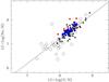 |
Fig. 1 12 + log (O / H) vs. 12 + log (Ne / H) in PNe in M33 (black triangles), M81 (red squares), and NGC 300 (blue filled circles). PNe in Local Group dwarf galaxies are shown as empty circles. The continuous line is the linear fit of the abundances of PNe in the whole sample of galaxies, while the dotted line is Izotov et al. (2006) fit of star-forming galaxies. |
Properties of the galaxy sample.
Details of the observations of the considered samples.
However, it is not possible to determine the exact range of progenitor mass for the PNe of each class. From observations, the minimum progenitor mass for a Type I PN is ~2 M⊙ (Peimbert & Serrano 1980), and for Type II PN is 1.2 M⊙ (Perinotto et al. 2004). From stellar evolution models, the mass range seems to be correlated with metallicity with the Type I PN mass cutoff (i.e. the critical mass for hot bottom burning) decreasing with metallicity. The population of extragalactic PNe is very similar to that of Galactic PNe, apart from a weak metallicity shift in the limit mass for Type I PN progenitors. The initial mass function (IMF) favours lower mass stars, thus Type I PNe are generally scarce in any galaxy. Furthermore, the evolution of the most massive post-AGB stars is very fast, making the corresponding PN shine for only a few years. Therefore, Type I PNe in external galaxies are a very small young population contaminant to the whole PN sample. Type III PNe are typically not observed in spiral galaxies, since they do not trace the spiral arms, where spectroscopic targets are typically chosen. Furthermore, in extragalactic samples one normally observes only the brightest first or second bins of the PN luminosity function (PNLF), which excludes Type III PNe (because they do not reach high luminosity), so most samples are populated by Type II PNe. In the present work, we select non-Type I PNe from the original samples, thus most PNe have progenitor mass in the range 1.2 <M< 2 M⊙. This places our PNe at ~1–5 Gyr look-back time (Maraston 1998).
3. The sample
There are only four spiral galaxies (other than the Milky Way) in which both H ii region and PN abundances are obtained with the direct-method. They constitute our sample. The main properties of the four galaxies, including coordinates, distance, optical radius, inclination, position angle, heliocentric systemic velocity, and morphology, are listed in Table 1. The references for distance and optical radius are quoted in the Table, while for inclination, position angle, and morphology we adopt the values from HyperLeda3. For some galaxies, the heliocentric systemic velocity is determined as described in Sect. 4.1. The quoted value is the average of the velocities obtained from all the individual ellipses. For other galaxies, the value is obtained from HyperLeda. The sample galaxies have morphological types from very late (NGC 300 − Scd) to early type (M81 − Sab). M31 and M33 belong to the Local Group. The M33 galaxy does not have strong interactions with dwarf companions, although it might have had some mutual interaction with M31 in the past (McConnachie et al. 2009; Putman et al. 2009). The M31 galaxy has several companions that might perturb its dynamics (Chemin et al. 2009; Dierickx et al. 2014). NGC 300 is relatively isolated, though traditionally considered a part of the Sculptor group. Finally, M81 is the largest galaxy of the M81 group and it is strongly interacting with its two brightest companions, M82 and NGC 3077, located within a short projected distance (60 kpc; Kaufman et al. 1989). The distribution of atomic hydrogen shows several extended tidal streams between M81 and its companions (Yun et al. 1994; Allen et al. 1997), which might be the result of close encounters ~200–300 Myr ago. In addition, M81 presents other peculiarities, as a reduced content of molecular gas with respect to other spiral galaxies (Casasola et al. 2004, 2007).
The PN and H ii region populations were previously studied via medium-resolution optical spectroscopy in all galaxies of our sample. In the following, we select abundance determinations via direct method for the reasons discussed in Sect. 2. We selected spectroscopic observations, which are all obtained with comparable telescopes and spectral resolutions, to produce a homogeneous sample of abundances. The details of the observations are shown in Table 2, including the reference for the determination of abundances, the telescope name (William Herschel Telescope, WHT; Multiple Mirror Telescope, MMT; and Very Large Telescope,VLT) with its diameter, spectral resolution, signal-to-noise ratio (S/N) of the faintest auroral lines, and typical uncertainties on the O abundance. In all datasets, the S/N is adequate for an accurate abundance analysis. In each galaxy, the uncertainties on O abundances from different literature sources are all comparable.
For M33 we adopt abundances of PNe from Magrini et al. (2009b, M09) and from Bresolin et al. (2010, hereafter B10), while for H ii regions from Magrini et al. (2007, 2010, hereafter M07 and M10, respectively) and references therein, and B10. For M31, the largest and most recent sample of H ii region abundances is computed by using strong-line ratios (Sanders et al. 2012, hereafter S12). For this galaxy we prefer to take advantage of the large sample of Sanders et al. (2012) of H ii region abundances and use the sample (Zurita & Bresolin 2012, hereafter Z12) with direct-method abundances to compute the offset between the direct method and the N2 = [Nii]/Hα calibration. For PNe, there are several studies focused on different PN populations of M31: PNe in the bulge and disc of M31 (Jacoby & Ciardullo 1999), in the very outer disc (Kwitter et al. 2012; Balick et al. 2013; Corradi et al. 2015), in the Northern Spur and the extension of the Giant Stream (Fang et al. 2013, 2015), and in the whole disc (Sanders et al. 2012). Since we are interested in the behaviour of the gradient within the optical radius, we consider here the abundance determination of Sanders et al. (2012) based on the direct method, including only PNe that kinematically belong to the disc population, i.e. excluding halo and satellite objects. There are several studies of H ii region abundances in M81, some based on the strong-line method (Garnett & Shields 1987; Bresolin et al. 1999) and others based on the direct method (Stanghellini et al. 2010; Patterson et al. 2012; Stanghellini et al. 2014; Arellano-Córdova et al. 2016). We adopt the direct-method results from Stanghellini et al. (2010, 2014, hereafter S10 and S14, respectively), and from Patterson et al. (2012, hereafter P12). In the case of the sample by Stanghellini et al. (2014), following their analysis, we include only H ii regions with uncertainties in O abundance <0.3 dex in our sample4. The only direct-method abundance determinations available for M81 PNe are those from Stanghellini et al. (2010), which we use in this paper. Finally for NGC 300, the O/H abundances of PNe and of H ii regions are from Stasińska et al. (2013, hereafter S13), and Bresolin et al. (2009, hereafter B09).
For all PN samples, since we are interested in the time evolution of the radial metallicity gradient, we have excluded, whenever possible, Type I PNe, keeping the PNe with the older progenitors.
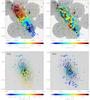 |
Fig. 2 Reconstructed two-dimensional fields of velocity (left panel) and velocity dispersion (right panel) for M31 (upper panels) and M33 (lower panels). Each cross represents the location of a detected PN and its colour indicates the value of ⟨ V ⟩ and ⟨ σ ⟩, as computed via the adaptive Gaussian kernel smoothing in that position. The spatial scale is given in arcsec. North is up; east is left. PNe in M31 that are denoted with an open circle were excluded from the analysis of the rotation curve and radial motions. |
 |
Fig. 3 Best-fit rotation curve (upper), velocity dispersion profile (middle), and radial motions (lower) of the PN population in M31 (left panel) and M33 (right panel). Black symbols show the results of fitting Eq. (1); green symbols refer to the results when fixing Vexp = 0; red triangles show the H i rotation curve as a comparison with M31 (Corbelli et al. 2010) and M33 (Corbelli & Salucci 2000). Positive values of Vexp correspond to outflowing motions for both galaxies. |
4. Migrating populations
Since PN progenitors have resided in the galaxy for several Gyr, it is essential to quantify their radial migration before proceeding in the analysis of gradient evolution. We need measurements of their velocity along the line of sight and proper motions; the latter is usually not available for extragalactic PNe. Within our galaxy sample, this analysis is possible only for M31 ad M33, which are the galaxies with the largest and most complete sample of PNe with accurate measurements of radial velocities. For M31, we combine the datasets of Sanders et al. (2012) and Merrett et al. (2006).
We use only disc PNe, i.e. we remove those PNe that are classified as H ii regions, halo PNe, or are associated with satellites5. This results in a sample of 731 PNe with measured radial velocity. For M33, we used the dataset of 140 disc PNe from Ciardullo et al. (2004).
We adopt two complementary approaches that should reveal the effects of different kind of radial motions. In the first approach (Sect. 4.1), we look for signatures of radial motions in the two-dimensional velocity field of the PN population. In the second approach (Sect. 4.2), we look for PNe that deviate from a simple rotational-disc model, and check whether their kinematics is consistent with radial motions. The first method is more sensitive to the presence of group of stars with an average radial component in their velocity vector; the second method is more sensitive to stars with a large radial component in their velocity (and small tangential component) and no net average radial motion.
4.1. Signatures of radial motions on the velocity field
The two-dimensional fields of velocity and velocity dispersion of PNe are recovered from the observations by smoothing the measured velocities v(x,y) with an adaptive Gaussian kernel along the spatial directions (Peng et al. 2004; Coccato et al. 2009). The size of the kernel represents a compromise between spatial resolution and number of PNe within the kernel that are needed to properly reconstruct the local line-of-sight velocity distribution (LOSVD). The kernel size automatically adapts according to the local PN number density; regions with higher concentration of PNe have smaller kernel size, whereas less populated regions have a larger kernel size (see Coccato et al. 2009, for details). The two-dimensional fields of the reconstructed velocity ⟨ V ⟩ and velocity dispersion ⟨ σ ⟩ are shown in Fig. 2.
Following the formalism by Teuben (2002), we model the galaxy velocity field ⟨ V ⟩ with a simple thin disc model that accounts for tangential Vrot (i.e. rotation) and expansion motions Vexp (i.e. radial migration, that can be inwards or outwards),  (1)where Vsys is the heliocentric systemic velocity, (R,θ) are polar coordinates in the plane of the galaxy, and (x,y) are cartesian coordinates in the plane of the sky (θ = 0 is aligned with the galaxy photometric major axis and corresponds to positive velocities along the line of sight, θ increases counter-clockwise). The relationship between the sky and the galaxy planes is given by
 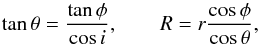 (2)where (r,φ) are polar coordinates in the plane of the sky. Inclinations of i = 72° and i = 55° were used for M31 and M33, respectively.
A positive value of Vexp translates into inwards or outwards motions depending on which side of the galaxy is the closest to us. This is determined by using the differential reddening of globular clusters. According to this method, the NW side of M31 is the closest to us (Iye & Richter 1985), whereas the SE side of M33 is the closest to us (Iye & Ozawa 1999). Taking our sign convention into account, this leads to outwards motions for positive values of Vexp in both galaxies.
We fit Eq. (1) in several elliptical bins to the reconstructed velocity field computed at the PN position for both galaxies. We kept Vsys the same for all of the bins. The boundaries of the bins are spaced according to an inverse hyperbolic sine function (Lupton et al. 1999). The value of R associated with a given bin is the median of all the values of R of all the PNe within that bin. The best-fitting semi-major axis profiles of Vrot(R) and Vexp(R) are shown in Fig. 3. For comparison, we show also the rotation curves of HI gas for M31 (Corbelli et al. 2010) and for M33 (Corbelli & Salucci 2000). Error bars are computed by means of Monte Carlo simulations in the following way: we constructed 1000 catalogues of simulated PNe that contain as many PNe as observed and located at the same position. The velocity of each simulated PN of coordinates (x,y) is randomly selected from a Gaussian distribution with mean value ⟨ V(x,y) ⟩ and dispersion [ ΔV2(x,y) + ⟨ σ ⟩ 2(x,y) ] 1 / 2, where ΔV(x,y) is the measurement error.
The rotation curve of M31 (left panels of Fig. 3) shows a rising profile reaching 100 km s-1 at 3 kpc (0.22°) followed by a plateau starting at ~6 kpc (0.45°). At larger radii, the scatter in the measured velocity increases. This is reflected by the local peaks in the velocity dispersion maps and by the presence of kinematic substructures in the velocity map (upper panels of Fig. 2). These features are probably due to the presence of small satellites that contaminated the PN disc population of M31. The majority of these features are offset from the galaxy photometric major axis; this explains the difference between our PN rotation curve and that shown by Merrett et al. (2006, their Fig. 33) in which only PNe closer than 0.04° to the major axis were considered. The profile of radial motions is consistent with 0 km s-1 up to ~7.5 kpc. For large radii, the contribution of radial motions to the mean velocity field of M31 becomes relevant, reaching ~100 km s-1 in modulus, despite the observed scatter. There is probably a non-negligible contribution from small satellites that are not identified in Merrett et al. (2006), but it is not possible to disentangle migrating PNe from satellite members with this technique.
In the case of M33, the rotation curve (right panels of Fig. 3) matches the rotational velocities of the PNe computed by Ciardullo et al. (2004, their Fig. 7a). It reaches a maximum amplitude of about ~60 km s-1 at ~5 kpc and then remains constant. The profile of radial motion shows large scatter with a weighted average of ⟨ Vexp ⟩ = −6 ± 7 km s-1 (about 6 kpc in 1 Gyr). Its radial velocity profile is consistent with 0 km s-1 at 1σ level for the majority of the bins (at 3σ level for all the bins, except for 22 bins 1 (~1 kpc) and 5 (~5.6 kpc)), where there is indication of radial inwards motions of about −12 km s-1.
Number of PNe in M31 that deviate more than 1σ from a pure rotating thin disc model compared with that expected from a pure Gaussian distribution for the elliptical bins.
Our analysis provides a strong indication that there is a significant Vexp component in the PN system of M31. On the other hand, our analysis provides only a weak indication (at 1σ level) that the Vexp component is present in the 1st and 5th elliptical bins of M33. In our simple model, we have directly associated Vexp with radial motions. However, other deviations from circular motions, such as elliptical streaming due to bar-like potential, spiral perturbations, and warp of the stellar disc, can mimic the presence of inwards or outwards motions (e.g. Wong et al. 2004, and references therein). Therefore, our measurements of the amplitude of radial motions should be considered upper limits. In the next section, we check whether the best-fit Vrot and Vexp are consistent with the individual measurements of PN velocities.
4.2. PNe that deviate from a pure rotating disc model
An independent analysis for evaluating radial motion in each elliptical bin is to count PNe that deviate from a pure rotating disc model. According to Sect. 4.1, we expect to observe deviating PNe outside 7.5 kpc in M31 and on the 1st and 5th elliptical bins of M33. We fit Eq. (1) to the measured PNe velocities v(x,y) in each elliptical bin setting Vexp = 0. We then count the number of PNe that deviate more than ⟨ σ ⟩ (a) in each bin, where ⟨ σ ⟩ (a) is the mean velocity dispersion in that bin. We then compare this value with that expected from a pure Gaussian LOSVD. The results are shown in Tables 3 and 4 for M31 and M33, respectively.
We found that all bins of M31 contain more kinematic outliers than expected by a Gaussian distribution. The measured ⟨ σ ⟩ represents an upper limit to the velocity dispersion of the disc PN population because of the probable presence of satellites. As a consequence, the estimated number of outliers in Table 3 is a lower limit to the actual value.
In Fig. 4 we show the azimuthal distribution of the PNe in M31 for the elliptical bin number 8, which is the bin with the largest number of outliers compared to the expected number. The corresponding figures for the other bins are shown in Appendix A. The figure shows that there are plenty of PNe whose line-of-sight velocity is consistent with being on radial migration. These are PNe with nearly 0 velocity, which are located at the position angles where the rotation is maximum, and PNe with high velocity, which are located at the position angles where the rotation is 0. Indeed, from Eq. (1) we expect the radial motions to be minimal (maximal) in correspondence of the position angles where the rotation is maximal (minimal).
In the same figure, we also show the location of PNe classified as halo or members of satellite systems (which are excluded from the fit). The majority of these PNe are clumped and well separated from the PNe associated with M31. However, there is some overlap between these systems, which can be responsible for some of the radial motions. Also, it is worth noticing that some of the PNe associated with M31 and that deviate from the circular model are clumped together. This indicates that these PNe are kinematically distinct from the PNe in the disc; whether this kinematic separation is entirely because of radial motions or because these PNe are to part of an (unknown) satellite is beyond the scope of this paper.
In M33, in contrast with Sect. 4.1, the 1st bin does not show more outliers than what is expected from a Gaussian distribution. Bin 5 has nine outliers, whereas eight are expected. Of those outliers, eight are located along the photometric major axis, where PNe in radial orbits should have zero velocity projected along the line of sight (LOS; see Eq. (1)). However, those eight PNe have a velocity that is much higher (in absolute value) than the systemic velocity. Therefore, their kinematics is not consistent with radial motions. One PN (in blue in Fig. 5) is located along the galaxy photometric minor axis. This is the direction where PNe in radial motions have LOS velocity higher than the systemic velocity. The positive sign of the velocity of that PN is consistent with outwards radial motions. However, this is in contrast with what is found in Sect. 4.1; radial motions in bin 5, if present, should be directed inwards. Similar arguments hold for bin 4, where an outlier (outside 3σ) is observed along the galaxy photometric minor axis and has a velocity 75 km s-1, consistent with outwards motions. However, the indication for bin 4th, if we ignore the error bar, is that motions are directed inwards.
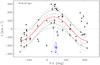 |
Fig. 4 Pure rotation disc model fit to PN velocities in M31 along the line of sight. The plot shows the fit for bin 8. The filled circles are the individual PN velocities v(x,y) expressed as function of the position angle on the sky (φ = 0 in Eq. (1) corresponds to PA = 35°; taken from the HyperLeda database). The red continuous curve represents the best-fitting rotation model, the red dashed lines are the model errors, as computed from the Monte Carlo simulations. Continuous black lines indicate the ± σ level, with the model errors indicated by black dashed lines. Black symbols refer to the analysed PN sample, blue symbols locate the discarded PNe: halo PNe, as defined by Sanders et al. (2012, filled blue circles), and satellite PNe, as identified by Merrett et al. (2006, open blue diamonds). |
The two different approaches give weak indications of the presence of radial motions in the PN population of M33, which are in contrast with each other. Even if we consider the upper limits of the radial motions found in our analysis, we can conclude that they do not imply a significant variation for the metallicity gradients of the PN population. In particular, a slight flattening could be produced by a global outwards motion, for which we estimate an upper limit of ~1 km s-1.6 This might be a significant amount, if integrated along the whole lifetime of a PN progenitor. However, the amount of PNe presently affected by radial migration does not exceed 7%, as estimated by the number of outliers in Table 3. The dramatic change in the slope of metallicity gradient foreseen by simulations (e.g. Roškar et al. 2008) can be obtained assuming that the migrating stars contribute to ≈50% of the total mass. These numbers are, however, not easy to compare with observations because our measurements describe possible migration at the current time, whereas the quantity in the simulations refers to the galaxy lifetime and many stars end up on circular orbits after migration. On the other hand, the effect of radial migration is more visible in the scatter of measurements rather that the slope itself (Grand et al. 2015).
In conclusion, our analysis supports the existence of significant radial motions in the PN system of M31. The present-time migration as measured from PNe and, especially, the considerable component of migrating PNe, might be compatible and responsible for the strong variation of the slope of the gradient, from that of PNe to that of H ii regions (see Table 5). On the other hand, our analysis does not support the existence of significant radial motions in the PN system of M33 at present time with a negligible effect compared to the uncertainties.
Gradients of the binned H ii regions and PN populations.
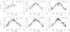 |
Fig. 5 Same as Fig. 4, but for all the elliptical bins of M33. The term φ = 0 in Eq. (1) corresponds to PA = −153° (taken from the HyperLeda database). |
5. The time-evolution of radial metallicity gradients
In order to determine time evolution of radial metallicity gradients, we proceed with the homogenisation of the literature samples in several ways:
1. Levelling out the radial scale. Spiral galaxies have different dimensions, which are often related to the morphological type also, where Sa galaxies are more extended that Sd galaxies. Several studies in the past have shown that the radial metallicity gradients can be related to several galactic properties, such as their morphology (e.g. McCall et al. 1985; Vila-Costas & Edmunds 1992), mass (e.g. Zaritsky et al. 1994; Martin & Roy 1994), presence of a bar (e.g. Zaritsky et al. 1994; Roy 1996), and interaction stage (e.g. Rupke et al. 2010). It has been claimed that the dependence on galaxy properties is only evident if the gradients are expressed in dex kpc-1 and the dependence disappears when expressed in unit of effective or optical radius. To make sure that the different scale lengths of galactic radii do not produce significant correlations with other galactic properties, a good approach is to use, for example the optical radius R25 (the 25 mag arcsec-2 isophotal ratio), the effective or half-light radius Re, or the disc scale length (the scale length of the exponential describing the profile of the disc), Rd . To this respect, it is worth noting that the works by Sánchez et al. (2014), Ho et al. (2015), Pilyugin et al. (2014), and (Bresolin & Kennicutt 2015), in which radial metallicity gradient slopes are expressed in terms of a reference radius, levelled the differences across galaxies.
The typical gradients of these works range from −0.12 dex / (R/Re) for Sánchez et al. (2014), to −0.39 ± 0.18 dex / (R/R25) for Ho et al. (2015), −0.32 ± 0.20 dex / (R/R25) for Pilyugin et al. (2014), and −0.045 ± 0.013 dex / (R/Rd) (O3N2 calibrator) for Bresolin & Kennicutt (2015). Sánchez et al. (2014), Ho et al. (2015), and Bresolin & Kennicutt (2015) express the gradients in different units; for instance, the Sánchez et al. (2014) gradient would be −0.20 ± 0.18 dex / (R/R25) if expressed in a R25 scale, as carried out by Ho et al. (2015) assuming an exponential disc with the typical central surface brightness for normal spirals and the empirical conversion between the different metallicity calibrations (Kewley & Ellison 2008).
While all the four examples mentioned above are based on strong-line abundances, there is purpose in comparing the gradients of galaxies of different morphological types based on a common physical scale, as, e.g. R25. In this way, we can also directly compare same-population gradients of different galaxies.
2. Binning the data. Smoothing the data in general provides a better idea of their behaviour. The binning procedure in the analysis of the radial metallicity gradients was performed, for example by Maciel & Quireza (1999) in their study of the gradient of PNe and by Huang et al. (2015) in their study of the red clump star gradient. The procedure gives more robustness to the data, removing possible local discrepancies and uncertainties, and defines an average abundance at each galactocentric distance. In addition, the procedure avoids giving too much weight to some regions in the parameter space where, for several reasons, we might have more data. Each bin is represented by the average abundances of all objects with distances between ± 0.05R/R25 from the central value. For each galaxy, the different literature sources give comparable errors, thus each data point was equally weighted to produce the final bin value. The error is the standard deviation of the mean.
3. Comparing common radial bins. In the CALIFA sample, the gradients of many galaxies show evidence of a flattening beyond ~2 disc effective radii. This is consistent with several spectroscopic studies of external galaxies (e.g. Bresolin et al. 2009, 2012) and of our own Galaxy (e.g. Magrini et al. 2009a; Lépine et al. 2011; Huang et al. 2015). So, the comparison of different radial regions can lead to misleading results, especially if some of them include the very external part of the galactic discs. In the following, we compare similar radial ranges for the H ii region and PN population in each galaxy, excluding bins outside ~R25 where possible changes of slopes might occur.
6. Results
6.1. Individual galaxies
In Figs. 6–9 we show the results of our analysis. In the upper panels of each figure, we show the individual measurements, and the gradients are obtained from the linear weighted fit of binned data and original literature gradients. In the lower panels, we present the binned abundances with their linear weighted fits.
NGC 300. Figure 6 shows the results for NGC 300. We did not include the two outermost H ii region bins in the fit, since there are no observed PNe in the corresponding bins. Their exclusion explains the small difference with the gradients derived by Stasińska et al. (2013). As already noticed by Stasińska et al. (2013), there is a clear difference in the slopes of the H ii region and PN gradients; the gradient in H ii regions is steeper than the PN gradient. For this galaxy, we cannot evaluate the effect of radial migration, thus the measured steepening with time is an upper limit; the gradient of PNe could have been steeper than the observed gradient.
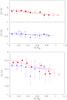 |
Fig. 6 NGC 300. Upper panel: individual and binned results for H ii regions (red circles and crosses for binned and individual results, respectively) and PNe (blue triangles and crosses for binned and individual results, respectively) in NGC 300. The O abundances of PNe and H ii regions are from Stasińska et al. (2013) and Bresolin et al. (2009). The dashed black lines are the gradients of Stasińska et al. (2013). The continuous lines are weighted linear fits computed in the radial regions where both populations are available. The typical errors in O/H for each dataset are shown on the right side of each panel. Lower panel: weighted linear fits of PN and H ii regions binned metallicities as in the upper panel. Each point corresponds to the average metallicity of the PN or H ii region population in a radial bin of 0.1R/R25. Empty symbols are for radial positions outside R25 or for populations that have no correspondence in the other sample (excluded from the fits). Dotted lines indicate the errors on the slopes and intercepts. |
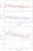 |
Fig. 7 M33. Upper panel: individual and binned results for H ii regions (upper panel) and PNe (lower panel) in M33. The O abundances of PNe are from Magrini et al. (2009b) and Bresolin et al. (2010; blue stars) and of H ii regions from Magrini et al. (2007, 2010) and references therein, and Bresolin et al. (2010; red crosses). The continuous black lines are the gradient of Magrini et al. (2010) for H ii regions (their whole sample) and the non-Type I PN sample of Magrini et al. (2009b) in the upper and lower panels, respectively. Lower panel: weighted linear fits of PN and H ii region binned metallicities. Symbols and curves as in Fig. 6. |
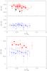 |
Fig. 8 M31. Upper panel: individual and binned results for H ii regions (upper panel) and PNe (lower panel) in M31. The O abundances of PNe are from Sanders et al. (2012; blue stars) and those of H ii regions are from Zurita & Bresolin (2012; black empty stars) and from Sanders et al. (2012; red crosses). The black filled circles are the H ii regions binned metallicities of Zurita & Bresolin (2012). Lower panel: weighted linear fits of PN and H ii region binned metallicities. Symbols and curves as in Fig. 6. |
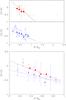 |
Fig. 9 M81. Upper panel: individual and binned results for H ii regions (upper panel) and PNe (lower panel). The O abundances of PNe are taken from Stanghellini et al. (2010) and those of H ii regions from Stanghellini et al. (2010, 2014) and Patterson et al. (2012). The continuous black lines are the gradient of Stanghellini et al. (2014) for PNe and that of Stanghellini et al. (2014) for H ii regions. Lower panel: weighted linear fits of PN and H ii region binned metallicities. Symbols and curves as in Fig. 6. |
M33. Figure 7 shows the results for M33. In this case, we excluded on the outermost bin in the PN sample. As already noticed by Magrini et al. (2010), the PN and H ii region gradients are indistinguishable within the errors, and present only an offset in metallicity. For M33 the effect of radial migration is negligible, and thus the comparison between the two populations shows the “true” evolution of the gradient, which is null or extremely small.
M31. The gradients of M31 are shown in Fig. 8. In the first panel, we show also the direct-method abundances of Zurita & Bresolin (2012) for a small number of H ii regions. These abundances are much lower that those derived by Sanders et al. (2012) with the N2 indicator. This is a well-known systematic effect as a result of strong-line vs. direct methods (e.g. Kewley & Dopita 2002). However, the slopes of the gradient in the radial region where the two methods overlap are in rough agreement with the gradient from the direct method; the latter method is slightly steeper. As shown by Stanghellini et al. (2015), the strong-line abundances can indeed give “first order” constraints to galactic evolutionary models, even if more uncertain than the direct-method abundances. In the case of M31, the best that we can do is to use the slope derived by the larger sample of Sanders et al. (2012), thus with a better statistics, rescaling the value of the intercept by the average difference of the two bins in common between Zurita & Bresolin (2012) and Sanders et al. (2012). In the lower panel, we compare the PN and H ii region gradients. As in the case of NGC 300, and even more evidently, the gradient of H ii regions is steeper that of that of the PN population. However, we recall that for this galaxy we are able to estimate the effects of radial migration. These effects are particularly important at ~8 kpc, corresponding to ~0.4R/R25 in the R25 scale. This is exactly where we observe an increase in the scatter of the PN abundances and where the radial gradient of PNe show a “jump” of about ~0.2 dex. Thus, the steepening with time of the slope of the gradient and the large scatter could be, in part, attributed to the radial migration of its PN population.
M81. The results for M81 are shown in Fig. 9. As for the other galaxies examined, the PN gradient is flatter than that of the H ii regions, as already noticed by Stanghellini et al. (2014). As for NGC 300, no estimates of radial migration for this galaxy are available, thus the steepening with time can be attributed both to migration and to chemical evolution.
6.2. General findings
We summarise all gradients in Table 5. Our four galaxies have gradient slopes from the H ii region populations ranging from −0.22 dex / (R/R25) in M33 to −0.75 dex / (R/R25) in M81; PN gradients are generally flatter, from −0.08 dex / (R/R25) in M31 to −0.46 dex / (R/R25) in M81.
The first consideration regards the global enrichment of the galaxies, which can be approximated by the difference in the value of the intercepts in Table 5. The four galaxies have all increased their metallicity content from the epoch of the formation of PN progenitors to the present time. For M31, the intercept computed using the strong-line abundances of Sanders et al. (2012) cannot be directly compared to the PN abundances. Thus we have corrected it using the abundances obtained with the direct method by Zurita & Bresolin (2012); the new value yields an almost solar abundance. The metallicity enrichment ranges from + 0.05 dex in M33 to + 0.32 dex in M81. The results of the global enrichment are presented in the upper panel of Fig. 10, where the variations of the intercepts versus the morphological type are shown. Late morphological types have a smaller enrichment, while a higher enrichment occurs in early morphological types.
All galaxies of our sample present a small evolution of the gradient slope, which can be a simple uniform metallicity increase as in M33, or a steepening, as in NGC 300 and M31. From the present data, there is no observational evidence of gradients flattening with time. In the lower panel of Fig. 10, we present the variation of the gradient slope versus the morphological type. The most significant evolution occurs in early morphological types, while late types tend to have no or smoother evolution. In the case of M31, however, the radial migration of PNe has an important role in shaping the past gradient.
7. Discussion and comparison with models
It is important to compare our results with different kind of galactic chemical evolution models. We have selected two type of models: the classical chemical evolution models, specifically those of the grid of Mollá & Díaz (2005), and the cosmological models of Gibson et al. (2013) with a different treatment of the feedback.
In Fig. 11 we compare the gradients of the galaxies with the multiphase chemical evolution models of Mollá & Díaz (2005) for galaxies with different mass and star formation efficiencies. We excluded M81 because of the strong interaction and environmental effects that prevent us from comparing this galaxy with models of isolated galaxies. We selected the most appropriate model on the basis of the total mass of each galaxy, including dark matter, from the grid of Mollá & Díaz (2005), varying the star formation efficiency. The adopted total masses are 2.2 × 10¹¹M⊙, 4.3 × 10¹¹M⊙, and 2.0 × 10¹²M⊙ for NGC 300, M33, and M31, respectively (Mollá & Díaz 2005).
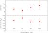 |
Fig. 10 Global enrichment (upper panel) and variation of the slope of the metallicity gradient (lower panel) as a function of the morphological type. |
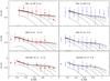 |
Fig. 11 Comparison with the multiphase chemical evolution models of Mollá & Díaz (2005) for galaxies with different mass and star formation efficiencies. Left panels: models at the present time (T = 13 Gyr). Right panels: models at the epoch of PN formation (T = 8 Gyr). Each curve is for a given star formation efficiency. For each galaxy, we chose the most appropriate mass distribution indicated with N in the plots, where N is the designation of the model in Table 1 of Mollá & Díaz (2005). |
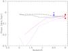 |
Fig. 12 Comparison of the redshift evolution of the gradient with the chemical evolution models of Gibson et al. (2013); black (dashed and dot-dashed) lines are models with enhanced feedback from SNe, magenta (short-dashed and dotted) lines are models with normal feedback. Red circles and blue triangles show the slopes of the gradients from H ii regions and PNe with 1.2 M⊙ progenitors, respectively. In this plot the slopes are expressed in dex/kpc for comparison with the models of Gibson et al. (2013). |
In the figure, we indicate with N the model of Table 1 of Mollá & Díaz (2005) to which we are referring, while the different curves corresponds to different sets of molecular cloud and star formation efficiencies; these range from 0.007 to 0.95 for the cloud formation efficiency and to 4 × 10⁻⁶ to 0.088 for the star formation efficiency.
The left-hand panels show the present-time models and H ii region abundances, while the right-hand panels show models at roughly the time of the formation of the oldest PN progenitors, i.e. about 5 Gyr ago, and PN abundances. In general, the agreement between the H ii region gradients and the present-time modelled gradients is satisfactory for the models with the highest star formation efficiency (from 0.14 to 0.88). Lower star formation efficiencies (from 0.05 to 4 × 10⁻⁶) produce gradients with shorter scale lengths. For NGC 300 and M33, the observed PN gradients and the models are very close, whereas for M31 the result from the old population is flatter than any modelled galaxy. In this galaxy, radial migration is important and can contribute to the flattening of the PN gradient.
We note that in Fig. 11 the modelled radial metallicity gradient, and likely the “real” gradients, are far from being approximated by a single slope. Probably, our simplistic assumption of a single slope gradient hides a more complex time evolution of the metallicity distribution, in which, for instance, inner and outer regions do not evolve at the same rate.
In Fig. 12, we compare the cosmological models of Gibson et al. (2013) with different treatment of the feedback, that is “enhanced” and “conservative” feedbacks, with our gradient slopes from H ii regions and PNe. The models are built to reproduce the present-time gradient of a Milky-Way-like galaxy, therefore it is not surprising that the agreement with the H ii regions gradient is good. The range of values for our H ii region gradients indicates the dependence on the morphological type when the gradients are expressed in terms of dex kpc-1. On the other hand, the gradients traced by PNe put important constraints on the models; the current data certainly favour a smooth evolution of the gradient and are not consistent with a flatter gradient in the past in the time lapse (and redshift interval) constrained by PNe. Comparing the data with the two sets of models, that is “enhanced” and “conservative” feedbacks, at the epoch of birth of PNe, we can discern a better agreement with the first class of models in which the energy of SNe is widely redistributed. All PN gradients in this plot have been placed at 5 Gyr, corresponding to progenitor mass at turnoff of 1.2 M⊙ (Maraston 1998). This is the lower limit of masses of Type II PNe, favoured by the IMF, but may not strictly represent the progenitor mass/look-back time for all PN within each sample. Each PN sample can be contaminated by a few Type III PNe, which would probe higher redshifts (0.5 <z< 8). On the other hand, we have excluded Type I PNe, as discussed above. With cosmological parameters H0 = 67.04 km s-1 Mpc-1, Ωm = 0.3183, ΩΛ = 0.6817, this look-back time corresponds to a redshift of z ≃ 0.5.
It is clear from the plot that extragalactic PNe cannot trace the most remote past of galaxies, probing the epochs where the two scenarios mostly differ. For example, one of the models with more conservative feedback (the dashed magenta curve in Fig. 12) is still consistent, within the errors, with the observational constraints from PNe. It is worth noting that Type III Galactic PNe probe a look-back time up to 8 Gyr, and that the Type III PN gradient observed in the Galaxy (Stanghellini & Haywood 2010) also agrees with the enhanced feedback models (see Gibson et al. 2013). Nonetheless, the Galactic PN gradient suffers from uncertainties in the distance scale, which make this constraint not very strong. For these reasons, local Universe constraints need to be complemented with high-redshift observations, as those of Cresci et al. (2010), Jones et al. (2010, 2013, 2015), and Yuan et al. (2011), which are able to shed light on the very early phases of disc evolution.
8. Summary
In the present work, we have analysed in a homogeneous way the literature data on direct-method abundances of H ii regions and PNe in four nearby disc galaxies: NGC 300, M33, M31, and M81. The abundances of H ii regions in M31 are an important exception, since only very few regions have direct-method abundances (Zurita & Bresolin 2012), while a large sample with abundances derived with strong lines is available (Sanders et al. 2012). In this case, we take advantage of the large sample of Sanders et al. (2012) and we use the sample of Zurita & Bresolin (2012) to compute the offset between the direct method and the strong-line calibration.
The analysed galaxies belong to different morphological types and allow us to study the time evolution of the metallicity enrichment and of the gradient as a function of galaxy morphology assuming that no correction is needed for the slope for stellar migration. To properly exploit PNe as tracers of the past composition of the ISM, we proved that their O abundances are unchanged at first order during the progenitor stellar evolution. Moreover, we estimated the amplitude of radial migration of the two galaxies in the sample with measured radial velocities. In the case of M33, we showed that the effects of radial migration on the metallicity gradients are negligible. In the case of M31, the effects of radial migration in the PN velocity field are non-negligible, and could have affected significantly the radial metallicity gradient in the last few Gyr.
Using H ii regions and PNe as tracers of the time evolution of the metallicity distribution in disc galaxies, we found that: (i) all galaxies are subject to a global oxygen enrichment with time that is higher for earlier type spirals (Sa-Sb). (ii) On average, the O/H gradients of the older population are equal to or flatter than those of H ii regions. While steeper O/H gradients for young populations have been noted before in spiral galaxies from direct abundances of PNe and H ii regions (Magrini et al. 2009b; Stasińska et al. 2013; Stanghellini et al. 2014), we confirm this trend when galaxies are studied in a comparable radial domain and metallicity binning. (iii) Our kinematical study of PNe in M33 and in M31 finds that radial migration can contribute to the observed flattening, especially in the case of M31. The undisturbed PN population of M33 allows us to better constrain the time evolution of the radial gradient.
Our radial gradients and their time evolution are compared with classical and cosmological chemical evolution models. They are found to be in good agreement with the multiphase chemical evolution models by Mollá & Díaz (2005). Using our results as constraints to the cosmological models of galaxy evolution of Gibson et al. (2013), we find that, in the redshift range sampled by H ii regions and PNe, models with enhanced SN feedback are favoured.
With the current technology, the realm of star-forming galaxies, where the time evolution of the metallicity gradient evolution can be obtained from direct-method abundances, is limited. By setting a limit from the PNLFs studied so far and reasonable observability in a few 8 m-class telescope nights, we expect to enlarge our sample by few more galaxies. This would allow us to refine the evolutionary trends shown in Fig. 12. We also expect to acquire in the near future deeper spectra of the current galaxies, to better characterise their PN and H ii region populations, as for instance in M31, and possibly to reveal older PN populations. However, the strongest constraints to the galactic evolutionary models are expected to come from either a better determination of the distance scale for Galactic PNe, to which the Gaia satellite will contribute, from abundance studies of high-redshift galaxies and from the future 30 m-class telescopes. The latter will favour both better characterisation of PNe and H ii regions in the nearby galaxies with optical multi-object spectroscopy and abundances of redshifted galaxies with infrared integral field unit spectroscopy.
It is worth noting that not all Galactic tracers indicate that the radial metallicity gradients are flat in the outer parts of the Galactic disc. For example, Cepheid gradients (Luck et al. 2011; Lemasle et al. 2013) seem to be negative at all radii.
For M31, only the O abundance is available in Sanders et al. (2012).
We excluded from our sample the abundances of Arellano-Córdova et al. (2016) because of an alternate approach in deriving oxygen abundances with different temperatures for different ions based on a relation between [Oiii] and [Nii] Te (e.g. Esteban et al. 2009) with respect to Stanghellini et al. (2010), Patterson et al. (2012), Stanghellini et al. (2014), who used only measured temperatures for all ions.
Sanders et al. (2012) have identified halo PNe in their sample on the basis of their position along the minor axis (| Y | > 4 kpc). Merrett et al. (2006) have identified those PNe that belong to satellites or background galaxies in their sample on the basis of their measured velocities and their proximity to known systems (M32, M110, Andromeda IV and VIII, 2MASXi J0039374+420956, and MLA93 0953) (see Sect. 7 of Merrett et al. (2006) for more details).
The upper limit is estimated from ⟨ Vexp ⟩ = (−6 ± 7) km s-1.
Acknowledgments
The authors are very grateful to the referee for her/his constructive report that improved the quality and presentation of the paper. This research has made use of the NASA/IPAC Extragalactic Database (NED) which is operated by the Jet Propulsion Laboratory, California Institute of Technology, under contract with the National Aeronautics and Space Administration. We acknowledge the usage of the HyperLeda database. V.C. acknowledges DustPedia, a collaborative focused research project supported by the European Union under the Seventh Framework Programme (2007−2013) call (proposal No. 606824). The participating institutions are Cardiff University, UK; National Observatory of Athens, Greece; Ghent University, Belgium; Université Paris Sud, France; National Institute for Astrophysics, Italy; and CEA (Paris), France.
References
- Allen, R. J., Knapen, J. H., Bohlin, R., & Stecher, T. P. 1997, ApJ, 487, 171 [NASA ADS] [CrossRef] [Google Scholar]
- Aller, L. H. 1942, ApJ, 95, 52 [NASA ADS] [CrossRef] [Google Scholar]
- Andrievsky, S. M., Luck, R. E., Martin, P., & Lépine, J. R. D. 2004, A&A, 413, 159 [NASA ADS] [CrossRef] [EDP Sciences] [Google Scholar]
- Arellano-Córdova, K. Z., Rodríguez, M., Mayya, Y. D., & Rosa-González, D. 2016, MNRAS, 455, 2627 [NASA ADS] [CrossRef] [Google Scholar]
- Balick, B., Kwitter, K. B., Corradi, R. L. M., & Henry, R. B. C. 2013, ApJ, 774, 3 [NASA ADS] [CrossRef] [Google Scholar]
- Balser, D. S., Rood, R. T., Bania, T. M., & Anderson, L. D. 2011, ApJ, 738, 27 [NASA ADS] [CrossRef] [Google Scholar]
- Berg, D. A., Skillman, E. D., Marble, A. R., et al. 2012, ApJ, 754, 98 [NASA ADS] [CrossRef] [Google Scholar]
- Berg, D. A., Skillman, E. D., Garnett, D. R., et al. 2013, ApJ, 775, 128 [NASA ADS] [CrossRef] [Google Scholar]
- Berg, D. A., Skillman, E. D., Croxall, K. V., et al. 2015, ApJ, 806, 16 [Google Scholar]
- Bono, G., Caputo, F., Marconi, M., & Musella, I. 2010, ApJ, 715, 277 [NASA ADS] [CrossRef] [Google Scholar]
- Bresolin, F. 2007, ApJ, 656, 186 [NASA ADS] [CrossRef] [Google Scholar]
- Bresolin, F., & Kennicutt, R. C. 2015, MNRAS, 454, 3664 [NASA ADS] [CrossRef] [Google Scholar]
- Bresolin, F., Kennicutt, R. C., Jr., & Garnett, D. R. 1999, ApJ, 510, 104 [NASA ADS] [CrossRef] [Google Scholar]
- Bresolin, F., Gieren, W., Kudritzki, R.-P., et al. 2009, ApJ, 700, 309 [NASA ADS] [CrossRef] [Google Scholar]
- Bresolin, F., Stasińska, G., Vílchez, J. M., Simon, J. D., & Rosolowsky, E. 2010, MNRAS, 404, 1679 [NASA ADS] [Google Scholar]
- Bresolin, F., Kennicutt, R. C., & Ryan-Weber, E. 2012, ApJ, 750, 122 [NASA ADS] [CrossRef] [Google Scholar]
- Brook, C. B., Stinson, G., Gibson, B. K., Wadsley, J., & Quinn, T. 2012, MNRAS, 424, 1275 [NASA ADS] [CrossRef] [Google Scholar]
- Casasola, V., Bettoni, D., & Galletta, G. 2004, A&A, 422, 941 [NASA ADS] [CrossRef] [EDP Sciences] [Google Scholar]
- Casasola, V., Combes, F., Bettoni, D., & Galletta, G. 2007, A&A, 473, 771 [NASA ADS] [CrossRef] [EDP Sciences] [Google Scholar]
- Chemin, L., Carignan, C., & Foster, T. 2009, ApJ, 705, 1395 [NASA ADS] [CrossRef] [Google Scholar]
- Chen, L., Hou, J. L., & Wang, J. J. 2003, AJ, 125, 1397 [NASA ADS] [CrossRef] [Google Scholar]
- Chiappini, C., Matteucci, F., & Romano, D. 2001, ApJ, 554, 1044 [NASA ADS] [CrossRef] [Google Scholar]
- Chieffi, A., & Limongi, M. 2004, ApJ, 608, 405 [NASA ADS] [CrossRef] [Google Scholar]
- Ciardullo, R., Durrell, P. R., Laychak, M. B., et al. 2004, ApJ, 614, 167 [Google Scholar]
- Coccato, L., Gerhard, O., Arnaboldi, M., et al. 2009, MNRAS, 394, 1249 [NASA ADS] [CrossRef] [Google Scholar]
- Corbelli, E., & Salucci, P. 2000, MNRAS, 311, 441 [NASA ADS] [CrossRef] [Google Scholar]
- Corbelli, E., Lorenzoni, S., Walterbos, R., Braun, R., & Thilker, D. 2010, A&A, 511, A89 [NASA ADS] [CrossRef] [EDP Sciences] [Google Scholar]
- Corradi, R. L. M., Kwitter, K. B., Balick, B., Henry, R. B. C., & Hensley, K. 2015, ApJ, 807, 181 [NASA ADS] [CrossRef] [Google Scholar]
- Cresci, G., Mannucci, F., Maiolino, R., et al. 2010, Nature, 467, 811 [NASA ADS] [CrossRef] [PubMed] [Google Scholar]
- Daflon, S., & Cunha, K. 2004, ApJ, 617, 1115 [NASA ADS] [CrossRef] [Google Scholar]
- Deharveng, L., Peña, M., Caplan, J., & Costero, R. 2000, MNRAS, 311, 329 [NASA ADS] [CrossRef] [Google Scholar]
- Delgado-Inglada, G., Morisset, C., & Stasińska, G. 2014, MNRAS, 440, 536 [NASA ADS] [CrossRef] [Google Scholar]
- Dierickx, M., Blecha, L., & Loeb, A. 2014, ApJ, 788, L38 [NASA ADS] [CrossRef] [Google Scholar]
- Di Matteo, P., Haywood, M., Combes, F., Semelin, B., & Snaith, O. N. 2013, A&A, 553, A102 [NASA ADS] [CrossRef] [EDP Sciences] [Google Scholar]
- Draine, B. T., Aniano, G., Krause, O., et al. 2014, ApJ, 780, 172 [NASA ADS] [CrossRef] [Google Scholar]
- Edvardsson, B., Andersen, J., Gustafsson, B., et al. 1993, A&A, 275, 101 [NASA ADS] [Google Scholar]
- Esteban, C., García-Rojas, J., Peimbert, M., et al. 2005, ApJ, 618, L95 [NASA ADS] [CrossRef] [Google Scholar]
- Esteban, C., Bresolin, F., Peimbert, M., et al. 2009, ApJ, 700, 654 [NASA ADS] [CrossRef] [Google Scholar]
- Fang, X., Zhang, Y., García-Benito, R., Liu, X.-W., & Yuan, H.-B. 2013, ApJ, 774, 138 [NASA ADS] [CrossRef] [Google Scholar]
- Fang, X., Garcia-Benito, R., Guerrero, M. A., et al. 2015, ApJ, 815, 69 [NASA ADS] [CrossRef] [Google Scholar]
- Ferrini, F., Molla, M., Pardi, M. C., & Diaz, A. I. 1994, ApJ, 427, 745 [NASA ADS] [CrossRef] [Google Scholar]
- Freedman, W. L., Madore, B. F., Gibson, B. K., et al. 2001, ApJ, 553, 47 [NASA ADS] [CrossRef] [Google Scholar]
- Friel, E. D. 1995, ARA&A, 33, 381 [NASA ADS] [CrossRef] [Google Scholar]
- García-Rojas, J., & Esteban, C. 2007, ApJ, 670, 457 [NASA ADS] [CrossRef] [Google Scholar]
- Garnett, D. R., & Shields, G. A. 1987, ApJ, 317, 82 [NASA ADS] [CrossRef] [Google Scholar]
- Gerke, J. R., Kochanek, C. S., Prieto, J. L., Stanek, K. Z., & Macri, L. M. 2011, ApJ, 743, 176 [NASA ADS] [CrossRef] [Google Scholar]
- Gibson, B. K., Pilkington, K., Brook, C. B., Stinson, G. S., & Bailin, J. 2013, A&A, 554, A47 [NASA ADS] [CrossRef] [EDP Sciences] [Google Scholar]
- Goddard, Q. E., Bresolin, F., Kennicutt, R. C., Ryan-Weber, E. V., & Rosales-Ortega, F. F. 2011, MNRAS, 412, 1246 [NASA ADS] [Google Scholar]
- Gonçalves, D. R., Magrini, L., Leisy, P., & Corradi, R. L. M. 2007, MNRAS, 375, 715 [NASA ADS] [CrossRef] [Google Scholar]
- Gonçalves, D. R., Magrini, L., Martins, L. P., Teodorescu, A. M., & Quireza, C. 2012, MNRAS, 419, 854 [NASA ADS] [CrossRef] [Google Scholar]
- Gonçalves, D. R., Magrini, L., Teodorescu, A. M., & Carneiro, C. M. 2014, MNRAS, 444, 1705 [NASA ADS] [CrossRef] [Google Scholar]
- Grand, R. J. J., Kawata, D., & Cropper, M. 2015, MNRAS, 447, 4018 [NASA ADS] [CrossRef] [Google Scholar]
- Haywood, M. 2008, MNRAS, 388, 1175 [NASA ADS] [CrossRef] [Google Scholar]
- Hernández-Martínez, L., Peña, M., Carigi, L., & García-Rojas, J. 2009, A&A, 505, 1027 [NASA ADS] [CrossRef] [EDP Sciences] [Google Scholar]
- Henry, R. B. C., Kwitter, K. B., Jaskot, A. E., et al. 2010, ApJ, 724, 748 [NASA ADS] [CrossRef] [MathSciNet] [Google Scholar]
- Herwig, F. 2004, ApJS, 155,651 [NASA ADS] [CrossRef] [Google Scholar]
- Ho, I.-T., Kudritzki, R.-P., Kewley, L. J., et al. 2015, MNRAS, 448, 2030 [NASA ADS] [CrossRef] [Google Scholar]
- Hou, J. L., Prantzos, N., & Boissier, S. 2000, A&A, 362, 921 [NASA ADS] [Google Scholar]
- Huang, Y., Liu, X.-W., Zhang, H.-W., et al. 2015, RA&A, 15, 1240 [Google Scholar]
- Iye, M., & Richter, O.-G. 1985, A&A, 144, 471 [NASA ADS] [Google Scholar]
- Iye, M., & Ozawa, T. 1999, Galaxy Dynamics – A Rutgers Symposium, ASP Conf. Ser., 182 [Google Scholar]
- Izotov, Y. I., Stasińska, G., Meynet, G., Guseva, N. G., & Thuan, T. X. 2006, A&A, 448, 955 [NASA ADS] [CrossRef] [EDP Sciences] [Google Scholar]
- Jacoby, G. H., & Ciardullo, R. 1999, ApJ, 515, 169 [NASA ADS] [CrossRef] [Google Scholar]
- Jones, T., Ellis, R., Jullo, E., & Richard, J. 2010, ApJ, 725, L176 [NASA ADS] [CrossRef] [Google Scholar]
- Jones, T., Ellis, R. S., Richard, J., & Jullo, E. 2013, ApJ, 765, 48 [NASA ADS] [CrossRef] [Google Scholar]
- Jones, T., Wang, X., Schmidt, K. B., et al. 2015, AJ, 149, 107 [NASA ADS] [CrossRef] [Google Scholar]
- Karakas, A. I. 2010, MNRAS, 403, 1413 [NASA ADS] [CrossRef] [Google Scholar]
- Karakas, A., & Lattanzio, J. C. 2007, PASA, 24, 103 [NASA ADS] [CrossRef] [Google Scholar]
- Kaufman, M., Bash, F. N., Hine, B., et al. 1989, ApJ, 345, 674 [NASA ADS] [CrossRef] [Google Scholar]
- Kewley, L. J., & Dopita, M. A. 2002, ApJS, 142, 35 [NASA ADS] [CrossRef] [Google Scholar]
- Kewley, L. J., & Ellison, S. L. 2008, ApJ, 681, 1183 [NASA ADS] [CrossRef] [Google Scholar]
- Kingsburgh, R. L., & Barlow, M. J. 1994, MNRAS, 271, 257 [NASA ADS] [CrossRef] [Google Scholar]
- Kubryk, M., Prantzos, N., & Athanassoula, E. 2013, MNRAS, 436, 1479 [NASA ADS] [CrossRef] [Google Scholar]
- Kwitter, K. B., & Henry, R. B. C. 2001, ApJ, 562, 804 [NASA ADS] [CrossRef] [Google Scholar]
- Kwitter, K. B., Lehman, E. M. M., Balick, B., & Henry, R. B. C. 2012, ApJ, 753, 12 [NASA ADS] [CrossRef] [Google Scholar]
- Lépine, J. R. D., Cruz, P., Scarano, S., Jr., et al. 2011, MNRAS, 417, 698 [NASA ADS] [CrossRef] [Google Scholar]
- Liu, X.-W., Storey, P. J., Barlow, M. J., & Clegg, R. E. S. 1995, MNRAS, 272, 369 [NASA ADS] [CrossRef] [Google Scholar]
- Liu, X.-W., Storey, P. J., Barlow, M. J., et al. 2000, MNRAS, 312, 585 [NASA ADS] [CrossRef] [Google Scholar]
- Liu, X.-W., Luo, S.-G., Barlow, M. J., Danziger, I. J., & Storey, P. J. 2001, MNRAS, 327, 141 [NASA ADS] [CrossRef] [Google Scholar]
- Lemasle, B., François, P., Genovali, K., et al. 2013, A&A, 558, A31 [NASA ADS] [CrossRef] [EDP Sciences] [Google Scholar]
- Loebman, S. R., Debattista, V. P., Nidever, D. L., et al. 2016, ApJ, 818, L6 [NASA ADS] [CrossRef] [Google Scholar]
- Luck, R. E., Kovtyukh, V. V., & Andrievsky, S. M. 2006, AJ, 132, 902 [NASA ADS] [CrossRef] [Google Scholar]
- Luck, R. E., Andrievsky, S. M., Kovtyukh, V. V., Gieren, W., & Graczyk, D. 2011, AJ, 142, 51 [NASA ADS] [CrossRef] [Google Scholar]
- Lupton, R. H., Gunn, J. E., & Szalay, A. S. 1999, AJ, 118, 1406 [NASA ADS] [CrossRef] [Google Scholar]
- Maciel, W. J., & Quireza, C. 1999, A&A, 345, 629 [NASA ADS] [Google Scholar]
- Maciel, W. J., Costa, R. D. D., & Uchida, M. M. M. 2003, A&A, 397, 667 [NASA ADS] [CrossRef] [EDP Sciences] [Google Scholar]
- Magrini, L., & Gonçalves, D. R. 2009, MNRAS, 398, 280 [NASA ADS] [CrossRef] [Google Scholar]
- Magrini, L., Leisy, P., Corradi, R. L. M., et al. 2005, A&A, 443, 115 [NASA ADS] [CrossRef] [EDP Sciences] [Google Scholar]
- Magrini, L., Corbelli, E., & Galli, D. 2007, A&A, 470, 843 [NASA ADS] [CrossRef] [EDP Sciences] [Google Scholar]
- Magrini, L., Sestito, P., Randich, S., & Galli, D. 2009a, A&A, 494, 95 [NASA ADS] [CrossRef] [EDP Sciences] [Google Scholar]
- Magrini, L., Stanghellini, L., & Villaver, E. 2009b, ApJ, 696, 729 [NASA ADS] [CrossRef] [Google Scholar]
- Magrini, L., Stanghellini, L., Corbelli, E., Galli, D., & Villaver, E. 2010, A&A, 512, A63 [NASA ADS] [CrossRef] [EDP Sciences] [Google Scholar]
- Maraston, C. 1998, MNRAS, 300, 872 [NASA ADS] [CrossRef] [Google Scholar]
- Marigo, P. 2001, A&A, 370, 194 [NASA ADS] [CrossRef] [EDP Sciences] [Google Scholar]
- Martin, P., & Roy, J.-R. 1994, ApJ, 424, 599 [NASA ADS] [CrossRef] [Google Scholar]
- McCall, M. L., Rybski, P. M., & Shields, G. A. 1985, ApJS, 57, 1 [NASA ADS] [CrossRef] [Google Scholar]
- McConnachie, A. W., Irwin, M. J., Ibata, R. A., et al. 2009, Nature, 461, 66 [NASA ADS] [CrossRef] [PubMed] [Google Scholar]
- Merrett, H. R., Merrifield, M. R., Douglas, N. G., et al. 2006, MNRAS, 369, 120 [NASA ADS] [CrossRef] [Google Scholar]
- Minchev, I., & Famaey, B. 2010, ApJ, 722, 112 [NASA ADS] [CrossRef] [Google Scholar]
- Minchev, I., Famaey, B., Combes, F., et al. 2011, A&A, 527, A147 [NASA ADS] [CrossRef] [EDP Sciences] [Google Scholar]
- Minchev, I., Chiappini, C., & Martig, M. 2014, A&A, 572, A92 [NASA ADS] [CrossRef] [EDP Sciences] [Google Scholar]
- Mollá, M., & Díaz, A. I. 2005, MNRAS, 358, 521 [NASA ADS] [CrossRef] [Google Scholar]
- Osterbrock, D. E., & Ferland, G. J. 2006, Astrophysics of gaseous nebulae and active galactic nuclei, 2nd, eds. D. E. Osterbrock, & G. J. Ferland Sausalito (CA: University Science Books) [Google Scholar]
- Pagel, B. E. J., & Edmunds, M. G. 1981, ARA&A, 19, 77 [NASA ADS] [CrossRef] [Google Scholar]
- Patterson, M. T., Walterbos, R. A. M., Kennicutt, R. C., Chiappini, C., & Thilker, D. A. 2012, MNRAS, 422, 401 [NASA ADS] [CrossRef] [Google Scholar]
- Pedicelli, S., Bono, G., Lemasle, B., et al. 2009, A&A, 504, 81 [NASA ADS] [CrossRef] [EDP Sciences] [Google Scholar]
- Peimbert, M., & Serrano, A. 1980, Rev. Mex. Astron. Astrofis., 5, 9 [NASA ADS] [Google Scholar]
- Peimbert, M., Storey, P. J., & Torres-Peimbert, S. 1993, ApJ, 414, 626 [NASA ADS] [CrossRef] [Google Scholar]
- Peña, M., Stasińska, G., & Richer, M. G. 2007, A&A, 476, 745 [NASA ADS] [CrossRef] [EDP Sciences] [Google Scholar]
- Peng, E. W., Ford, H. C., & Freeman, K. C. 2004, ApJ, 602, 685 [NASA ADS] [CrossRef] [Google Scholar]
- Perinotto, M., Morbidelli, L., & Scatarzi, A. 2004, MNRAS, 349, 793 [NASA ADS] [CrossRef] [Google Scholar]
- Pilkington, K., Gibson, B. K., Brook, C. B., et al. 2012a, MNRAS, 425, 969 [NASA ADS] [CrossRef] [Google Scholar]
- Pilkington, K., Few, C. G., Gibson, B. K., et al. 2012b, A&A, 540, A56 [NASA ADS] [CrossRef] [EDP Sciences] [Google Scholar]
- Pilyugin, L. S., & Mattsson, L. 2011, MNRAS, 412, 1145 [NASA ADS] [Google Scholar]
- Pilyugin, L. S., Grebel, E. K., & Kniazev, A. Y. 2014, AJ, 147, 131 [NASA ADS] [CrossRef] [Google Scholar]
- Putman, M. E., Peek, J. E. G., Muratov, A., et al. 2009, ApJ, 703, 1486 [NASA ADS] [CrossRef] [Google Scholar]
- Quillen, A. C., Minchev, I., Bland-Hawthorn, J., & Haywood, M. 2009, MNRAS, 397, 1599 [NASA ADS] [CrossRef] [Google Scholar]
- Richer, M. G., & McCall, M. L. 2008, ApJ, 684, 1190 [NASA ADS] [CrossRef] [Google Scholar]
- Roškar, R., Debattista, V. P., Quinn, T. R., Stinson, G. S., & Wadsley, J. 2008, ApJ, 684, L79 [NASA ADS] [CrossRef] [Google Scholar]
- Roy, J.-R. 1996, IAU Colloq. 157: Barred Galaxies, 91, 63 [NASA ADS] [Google Scholar]
- Rudolph, A. L., Fich, M., Bell, G. R., et al. 2006, ApJS, 162, 346 [NASA ADS] [CrossRef] [Google Scholar]
- Rupke, D. S. N., Kewley, L. J., & Chien, L.-H. 2010, ApJ, 723, 1255 [NASA ADS] [CrossRef] [Google Scholar]
- Sánchez, S. F., Rosales-Ortega, F. F., Iglesias-Páramo, J., et al. 2014, A&A, 563, A49 [NASA ADS] [CrossRef] [EDP Sciences] [Google Scholar]
- Sanders, N. E., Caldwell, N., McDowell, J., & Harding, P. 2012, ApJ, 758, 133 [Google Scholar]
- Schönrich, R., & Binney, J. 2009, MNRAS, 396, 203 [NASA ADS] [CrossRef] [Google Scholar]
- Searle, L. 1971, ApJ, 168, 327 [NASA ADS] [CrossRef] [Google Scholar]
- Sellwood, J. A., & Binney, J. J. 2002, MNRAS, 336, 785 [NASA ADS] [CrossRef] [Google Scholar]
- Sestito, P., Bragaglia, A., Randich, S., et al. 2006, A&A, 458, 121 [NASA ADS] [CrossRef] [EDP Sciences] [Google Scholar]
- Stanghellini, L., & Haywood, M. 2010, ApJ, 714, 1096 [NASA ADS] [CrossRef] [Google Scholar]
- Stanghellini, L., Magrini, L., Villaver, E., & Galli, D. 2010, A&A, 521, A3 [NASA ADS] [CrossRef] [EDP Sciences] [Google Scholar]
- Stanghellini, L., Magrini, L., Casasola, V., & Villaver, E. 2014, A&A, 567, A88 [NASA ADS] [CrossRef] [EDP Sciences] [Google Scholar]
- Stanghellini, L., Magrini, L., & Casasola, V. 2015, ApJ, 812, 39 [NASA ADS] [CrossRef] [Google Scholar]
- Stasińska, G., Peña, M., Bresolin, F., & Tsamis, Y. G. 2013, A&A, 552, A12 [NASA ADS] [CrossRef] [EDP Sciences] [Google Scholar]
- Stinson, G. S., Bailin, J., Couchman, H., et al. 2010, MNRAS, 408, 812 [NASA ADS] [CrossRef] [Google Scholar]
- Stinson, G. S., Brook, C., Macciò, A. V., et al. 2013, MNRAS, 428, 129 [NASA ADS] [CrossRef] [Google Scholar]
- Teuben, P. J. 2002, Discs of Galaxies: Kinematics, Dynamics and Peturbations, 275, 217 [Google Scholar]
- Tsamis, Y. G., Barlow, M. J., Liu, X.-W., Storey, P. J., & Danziger, I. J. 2004, MNRAS, 353, 953 [NASA ADS] [CrossRef] [Google Scholar]
- Tully, R. B., Courtois, H. M., Dolphin, A. E., et al. 2013, AJ, 146, 86 [NASA ADS] [CrossRef] [Google Scholar]
- van Zee, L., Skillman, E. D., & Haynes, M. P. 2006, ApJ, 637, 269 [NASA ADS] [CrossRef] [Google Scholar]
- Vila-Costas, M. B., & Edmunds, M. G. 1992, MNRAS, 259, 121 [NASA ADS] [CrossRef] [Google Scholar]
- Vilchez, J. M., & Esteban, C. 1996, MNRAS, 280, 720 [NASA ADS] [CrossRef] [Google Scholar]
- Werk, J. K., Putman, M. E., Meurer, G. R., & Santiago-Figueroa, N. 2011, ApJ, 735, 71 [NASA ADS] [CrossRef] [Google Scholar]
- Wong, T., Blitz, L., & Bosma, A. 2004, ApJ, 605, 183 [NASA ADS] [CrossRef] [Google Scholar]
- Woosley, S. E., & Weaver, T. A. 1995, ApJS, 101, 181 [NASA ADS] [CrossRef] [Google Scholar]
- Yong, D., Carney, B. W., Teixera de Almeida, M. L., & Pohl, B. L. 2006, AJ, 131, 2256 [NASA ADS] [CrossRef] [Google Scholar]
- Yuan, T.-T., Kewley, L. J., Swinbank, A. M., Richard, J., & Livermore, R. C. 2011, ApJ, 732, L14 [NASA ADS] [CrossRef] [Google Scholar]
- Yun, M. S., Ho, P. T. P., & Lo, K. Y. 1994, Nature, 372, 530 [NASA ADS] [CrossRef] [PubMed] [Google Scholar]
- Zaritsky, D., Kennicutt, R. C., Jr., & Huchra, J. P. 1994, ApJ, 420, 87 [NASA ADS] [CrossRef] [Google Scholar]
- Zurita, A., & Bresolin, F. 2012, MNRAS, 427, 1463 [NASA ADS] [CrossRef] [Google Scholar]
Appendix A: Circular model fit of M31
In this appendix, we show the circular model fit for all the elliptical bins in M31 as performed in Sect. 4.2.
All Tables
Number of PNe in M31 that deviate more than 1σ from a pure rotating thin disc model compared with that expected from a pure Gaussian distribution for the elliptical bins.
All Figures
|
Fig. 1 12 + log (O / H) vs. 12 + log (Ne / H) in PNe in M33 (black triangles), M81 (red squares), and NGC 300 (blue filled circles). PNe in Local Group dwarf galaxies are shown as empty circles. The continuous line is the linear fit of the abundances of PNe in the whole sample of galaxies, while the dotted line is Izotov et al. (2006) fit of star-forming galaxies. |
| In the text | |
|
Fig. 2 Reconstructed two-dimensional fields of velocity (left panel) and velocity dispersion (right panel) for M31 (upper panels) and M33 (lower panels). Each cross represents the location of a detected PN and its colour indicates the value of ⟨ V ⟩ and ⟨ σ ⟩, as computed via the adaptive Gaussian kernel smoothing in that position. The spatial scale is given in arcsec. North is up; east is left. PNe in M31 that are denoted with an open circle were excluded from the analysis of the rotation curve and radial motions. |
| In the text | |
|
Fig. 3 Best-fit rotation curve (upper), velocity dispersion profile (middle), and radial motions (lower) of the PN population in M31 (left panel) and M33 (right panel). Black symbols show the results of fitting Eq. (1); green symbols refer to the results when fixing Vexp = 0; red triangles show the H i rotation curve as a comparison with M31 (Corbelli et al. 2010) and M33 (Corbelli & Salucci 2000). Positive values of Vexp correspond to outflowing motions for both galaxies. |
| In the text | |
|
Fig. 4 Pure rotation disc model fit to PN velocities in M31 along the line of sight. The plot shows the fit for bin 8. The filled circles are the individual PN velocities v(x,y) expressed as function of the position angle on the sky (φ = 0 in Eq. (1) corresponds to PA = 35°; taken from the HyperLeda database). The red continuous curve represents the best-fitting rotation model, the red dashed lines are the model errors, as computed from the Monte Carlo simulations. Continuous black lines indicate the ± σ level, with the model errors indicated by black dashed lines. Black symbols refer to the analysed PN sample, blue symbols locate the discarded PNe: halo PNe, as defined by Sanders et al. (2012, filled blue circles), and satellite PNe, as identified by Merrett et al. (2006, open blue diamonds). |
| In the text | |
|
Fig. 5 Same as Fig. 4, but for all the elliptical bins of M33. The term φ = 0 in Eq. (1) corresponds to PA = −153° (taken from the HyperLeda database). |
| In the text | |
|
Fig. 6 NGC 300. Upper panel: individual and binned results for H ii regions (red circles and crosses for binned and individual results, respectively) and PNe (blue triangles and crosses for binned and individual results, respectively) in NGC 300. The O abundances of PNe and H ii regions are from Stasińska et al. (2013) and Bresolin et al. (2009). The dashed black lines are the gradients of Stasińska et al. (2013). The continuous lines are weighted linear fits computed in the radial regions where both populations are available. The typical errors in O/H for each dataset are shown on the right side of each panel. Lower panel: weighted linear fits of PN and H ii regions binned metallicities as in the upper panel. Each point corresponds to the average metallicity of the PN or H ii region population in a radial bin of 0.1R/R25. Empty symbols are for radial positions outside R25 or for populations that have no correspondence in the other sample (excluded from the fits). Dotted lines indicate the errors on the slopes and intercepts. |
| In the text | |
|
Fig. 7 M33. Upper panel: individual and binned results for H ii regions (upper panel) and PNe (lower panel) in M33. The O abundances of PNe are from Magrini et al. (2009b) and Bresolin et al. (2010; blue stars) and of H ii regions from Magrini et al. (2007, 2010) and references therein, and Bresolin et al. (2010; red crosses). The continuous black lines are the gradient of Magrini et al. (2010) for H ii regions (their whole sample) and the non-Type I PN sample of Magrini et al. (2009b) in the upper and lower panels, respectively. Lower panel: weighted linear fits of PN and H ii region binned metallicities. Symbols and curves as in Fig. 6. |
| In the text | |
|
Fig. 8 M31. Upper panel: individual and binned results for H ii regions (upper panel) and PNe (lower panel) in M31. The O abundances of PNe are from Sanders et al. (2012; blue stars) and those of H ii regions are from Zurita & Bresolin (2012; black empty stars) and from Sanders et al. (2012; red crosses). The black filled circles are the H ii regions binned metallicities of Zurita & Bresolin (2012). Lower panel: weighted linear fits of PN and H ii region binned metallicities. Symbols and curves as in Fig. 6. |
| In the text | |
|
Fig. 9 M81. Upper panel: individual and binned results for H ii regions (upper panel) and PNe (lower panel). The O abundances of PNe are taken from Stanghellini et al. (2010) and those of H ii regions from Stanghellini et al. (2010, 2014) and Patterson et al. (2012). The continuous black lines are the gradient of Stanghellini et al. (2014) for PNe and that of Stanghellini et al. (2014) for H ii regions. Lower panel: weighted linear fits of PN and H ii region binned metallicities. Symbols and curves as in Fig. 6. |
| In the text | |
|
Fig. 10 Global enrichment (upper panel) and variation of the slope of the metallicity gradient (lower panel) as a function of the morphological type. |
| In the text | |
|
Fig. 11 Comparison with the multiphase chemical evolution models of Mollá & Díaz (2005) for galaxies with different mass and star formation efficiencies. Left panels: models at the present time (T = 13 Gyr). Right panels: models at the epoch of PN formation (T = 8 Gyr). Each curve is for a given star formation efficiency. For each galaxy, we chose the most appropriate mass distribution indicated with N in the plots, where N is the designation of the model in Table 1 of Mollá & Díaz (2005). |
| In the text | |
|
Fig. 12 Comparison of the redshift evolution of the gradient with the chemical evolution models of Gibson et al. (2013); black (dashed and dot-dashed) lines are models with enhanced feedback from SNe, magenta (short-dashed and dotted) lines are models with normal feedback. Red circles and blue triangles show the slopes of the gradients from H ii regions and PNe with 1.2 M⊙ progenitors, respectively. In this plot the slopes are expressed in dex/kpc for comparison with the models of Gibson et al. (2013). |
| In the text | |
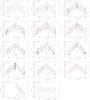 |
Fig. A.1 Same as Fig. 4, but for the remaining elliptical bins of M31. |
| In the text | |
Current usage metrics show cumulative count of Article Views (full-text article views including HTML views, PDF and ePub downloads, according to the available data) and Abstracts Views on Vision4Press platform.
Data correspond to usage on the plateform after 2015. The current usage metrics is available 48-96 hours after online publication and is updated daily on week days.
Initial download of the metrics may take a while.