| Issue |
A&A
Volume 587, March 2016
|
|
|---|---|---|
| Article Number | A39 | |
| Number of page(s) | 28 | |
| Section | Atomic, molecular, and nuclear data | |
| DOI | https://doi.org/10.1051/0004-6361/201527324 | |
| Published online | 15 February 2016 | |
Stellar laboratories
VI. New Mo iv–vii oscillator strengths and the molybdenum abundance in the hot white dwarfs G191−B2B and RE 0503−289⋆,⋆⋆,⋆⋆⋆
1 Institute for Astronomy and Astrophysics, Kepler Center for Astro and Particle Physics, Eberhard Karls University, Sand 1, 72076 Tübingen, Germany
e-mail: This email address is being protected from spambots. You need JavaScript enabled to view it.
2 Physique Atomique et Astrophysique, Université de Mons – UMONS, 7000 Mons, Belgium
3 IPNAS, Université de Liège, Sart Tilman, 4000 Liège, Belgium
4 Astronomisches Rechen-Institut, Zentrum für Astronomie, Ruprecht Karls University, Mönchhofstraße 12-14, 69120 Heidelberg, Germany
5 NASA Goddard Space Flight Center, Greenbelt, MD 20771, USA
Received: 8 September 2015
Accepted: 13 December 2015
Abstract
Context. For the spectral analysis of high-resolution and high signal-to-noise (S/N) spectra of hot stars, state-of-the-art non-local thermodynamic equilibrium (NLTE) model atmospheres are mandatory. These are strongly dependent on the reliability of the atomic data that is used for their calculation.
Aims. To identify molybdenum lines in the ultraviolet (UV) spectra of the DA-type white dwarf G191−B2B and the DO-type white dwarf RE 0503−289 and, to determine their photospheric Mo abundances, reliable Mo iv–vii oscillator strengths are used.
Methods. We newly calculated Mo iv–vii oscillator strengths to consider their radiative and collisional bound-bound transitions in detail in our NLTE stellar-atmosphere models for the analysis of Mo lines exhibited in high-resolution and high S/N UV observations of RE 0503−289.
Results. We identified 12 Mo v and 9 Mo vi lines in the UV spectrum of RE 0503−289 and measured a photospheric Mo abundance of 1.2−3.0 × 10⁻⁴ (mass fraction, 22 500−56 400 times the solar abundance). In addition, from the As v and Sn iv resonance lines, we measured mass fractions of arsenic (0.5−1.3 × 10⁻⁵, about 300−1200 times solar) and tin (1.3−3.2 × 10⁻⁴, about 14 300−35 200 times solar). For G191−B2B, upper limits were determined for the abundances of Mo (5.3 × 10⁻⁷, 100 times solar) and, in addition, for Kr (1.1 × 10⁻⁶, 10 times solar) and Xe (1.7 × 10⁻⁷, 10 times solar). The arsenic abundance was determined (2.3−5.9 × 10⁻⁷, about 21−53 times solar). A new, registered German Astrophysical Virtual Observatory (GAVO) service, TOSS, has been constructed to provide weighted oscillator strengths and transition probabilities.
Conclusions. Reliable measurements and calculations of atomic data are a prerequisite for stellar-atmosphere modeling. Observed Mo v-vi line profiles in the UV spectrum of the white dwarf RE 0503−289 were well reproduced with our newly calculated oscillator strengths. For the first time, this allowed the photospheric Mo abundance in a white dwarf to be determined.
Key words: atomic data / line: identification / stars: abundances / stars: individual: G191-B2B / stars: individual: RE0503-289 / virtual observatory tools
Based on observations with the NASA/ESA Hubble Space Telescope, obtained at the Space Telescope Science Institute, which is operated by the Association of Universities for Research in Astronomy, Inc., under NASA contract NAS5-26666.
Based on observations made with the NASA-CNES-CSA Far Ultraviolet Spectroscopic Explorer.
Tables A.10–A.13 are only available via the German Astrophysical Virtual Observatory (GAVO) service TOSS (http://dc.g-vo.org/TOSS).
© ESO, 2016
1. Introduction
RE 0503−289 (WD 0501−289, McCook & Sion 1999a,b) is a hot, helium-rich, DO-type white dwarf (WD, effective temperature Teff = 70 000 K, surface gravity log (g/ cm/s2) = 7.5, Dreizler & Werner 1996), that exhibits lines of at least ten trans-iron elements in its far-ultraviolet (FUV) spectrum (Werner et al. 2012b). The abundance analysis of these species is hampered by the lack of atomic data for their higher ionization stages, i.e., iv-vii. While Werner et al. (2012b) could measure only the Kr and Xe abundances, further abundance determinations (Zn, Ge, Ga, Xe, and Ba by Rauch et al. 2014a, 2012, 2014b, 2015b,a, respectively) were always initiated by new calculations of reliable transition probabilities.
G191−B2B (WD 0501+527, McCook & Sion 1999a,b) is a hot, hydrogen-rich, DA-type white dwarf that was recently analyzed by Rauch et al. (2013, Teff = 60 000 K, log g = 7.6. Based on this model, Rauch et al. (2014a,b, 2015b) measured the abundances of Zn, Ba, and Ga.
Molybdenum is another trans-iron element (atomic number Z = 42). It was discovered for the first time in a WD (in the spectrum of RE 0503−289) by Werner et al. (2012b, four Mo vi . To identify more lines of Mo and to determine its abundance, we calculated new transition probabilities for Mo iv–vii.
In this paper, we first describe the available observations (Sect. 2), our stellar-atmosphere models (Sect. 3), and the computation of the new transition probabilities (Sect. 4). A new Virtual Observatory (VO) service that provides access to transition probabilities is presented in Sect. 5.
To use the most elaborated models of G191−B2B and RE 0503−289 for our Mo abundance analysis, we start with an incorporation and an abundance determination of arsenic (Sect. 6.1, both stars) and tin (Sect. 6.2, RE 0503−289). Then, we assess the Mo photospheric abundances in RE 0503−289 and G191−B2B (Sect. 6.3). In Sect. 6.5, we determine upper abundance limits of krypton and xenon in G191−B2B. To understand the abundance patterns of trans-iron elements, we investigate on the efficiency of radiative levitation acting on the elements Zn, Ga, Ge, As, Kr, Mo, Sn, Xe, and Ba in both stars’ atmospheres (Sect. 7). We summarize our results and conclude in Sect. 8.
2. Observations
G191−B2B.
We used the spectra obtained with the Far Ultraviolet Spectroscopic Explorer (FUSE, 910 Å <λ< 1190 Å, resolving power R = λ/ Δλ ≈ 20 000, for details see Rauch et al. 2013) and the Hubble Space Telescope/Space Telescope Imaging Spectrograph (HST/STIS, 1145 Å <λ< 3145 Å, resolution of ≈3 km s-1, see Rauch et al. 20131).
RE 0503−289.
We analyzed its FUSE (described in detail by Werner et al. 2012b) and HST/STIS observations (1144 Å <λ< 3073 Å). The latter was co-added from two observations with grating E140M (exposure times 2493 s and 3001 s, 1144−1709 Å, R ≈ 45 800), and two observations with grating E230M (1338 s, 1690−2366 Å and 1338 s, 2277−3073 Å, R ≈ 30 000). These STIS observations are retrievable from the Barbara A. Mikulski Archive for Space Telescopes (MAST).
3. Model atmospheres and atomic data
We employed the Tübingen NLTE2 Model Atmosphere Package (TMAP3, Werner et al. 2003, 2012a) to calculate plane-parallel, chemically homogeneous model-atmospheres in hydrostatic and radiative equilibrium. Model atoms were taken from the Tübingen Model Atom Database (TMAD4, Rauch & Deetjen 2003) that has been constructed as part of the Tübingen contribution to the German Astrophysical Virtual Observatory (GAVO5). For our Mo model atoms, we follow Rauch et al. (2015b) and used a statistical approach to calculate so-called super levels and super lines with our Iron Opacity and Interface (IrOnIc6, Rauch & Deetjen 2003). We transferred our new Mo data into Kurucz-formatted files7 that were then ingested and processed by IrOnIc. The statistics of our Mo model atom is summarized in Table 1.
Statistics of Mo iv - vii atomic levels and line transitions from Tables A.10–A.13, respectively.
For Mo and all other species, level dissolution (pressure ionization) following Hummer & Mihalas (1988) and Hubeny et al. (1994) is accounted for. Broadening for all Mo lines that are due to the quadratic Stark effect is calculated using approximate formulae by Cowley (1970, 1971).
4. Atomic structure and radiative data calculation
New calculations of oscillator strengths for a large number of transitions of molybdenum ions that are considered in the present work were carried out using the pseudo-relativistic Hartree-Fock (HFR) method (Cowan 1981), including core-polarization corrections (see, e.g., Quinet et al. 1999, 2002).
For Mo iv, the configuration interaction was considered among the configurations 4d3, 4d25s, 4d26s, 4d25d, 4d26d, 4d4f2, 4d5s2, 4d5p2, 4d5d2, 4d5s5d, 4d5p4f, 4d5p5f, and 4d4f5f for the even parity and 4d25p, 4d26p, 4d24f, 4d25f, 4d5s5p, 4d5s4f, 4d5s5f, 4d5p5d, 4d4f5d, and 4d5d5f for the odd parity. The core-polarization parameters were the dipole polarizability of a Mo vii ionic core reported by Fraga et al. (1976), i.e., αd = 1.82 au, and the cut-off radius corresponding to the HFR mean value ⟨r⟩ of the outermost core orbital (4p), i.e., rc = 1.20 au. Using the experimental energy levels reported by Sugar & Musgrove (1988) and Cabeza et al. (1989), the radial integrals (average energy, Slater, spin-orbit and effective interaction parameters) of 4d3, 4d25s, 4d26s, 4d25d, and 4d25p configurations were adjusted by a well-established least-squares fitting process that minimizes the differences between computed and experimental energies.
For Mo v, the configurations retained in the HFR model were 4d2, 4d5s, 4d6s, 4d5d, 4d6d, 4d5g, 5s2, 5p2, 5d2, 4f2, 5s5d, 5s6s, 5p4f, 5p5f, 4p54d24f, 4p54d25f, and 4p54d25p for the even parity and 4d5p, 4d6p, 4d4f, 4d5f, 4d6f, 4d7f, 4d8f, 4d9f, 5s5p, 5p5d, 5s4f, 5s5f, 4f5d, 4p54d3, 4p54d25s, and 4p54d25d for the odd parity. In this ion, the semi-empirical process was performed to optimize the radial integrals corresponding to 4d2, 4d5s, 4d6s, 4d5d, 4d5g, 5s2, 5p2, 5s5d, 5s6s, 4d5p, 4d6p, 4d4f, 4d5f, 4d6f, 4d7f, 4d8f, 4d9f, 5s5p, 5s4f, and 4p54d3 configurations, which use the experimental energy levels reported by Reader & Tauheed (2015). Core-polarization effects were estimated using a dipole polarizability value corresponding to a Mo viii ionic core taken from Fraga et al. (1976), i.e., αd = 1.48 au, and a cut-off radius equal to 1.20 au.
In the case of Mo vi, the 4d, 5d, 6d, 7d, 8d, 5s, 6s, 7s, 8s, 5g, 6g, 7g, 8g, 7i, 8i, 4p54d5p, 4p54d4f, and 4p54d5f even configurations and the 5p, 6p, 7p, 8p, 9p, 10p, 11p, 4f, 5f, 6f, 7f, 8f, 9f, 6h, 7h, 8h, 8k, 4p54d2, 4p54d5s, and 4p54d5d odd configurations were explicitly included in the HFR model with the same core-polarization parameters as those considered for Mo v. The semi-empirical optimization process was carried out to fit the radial parameters in the nd (n = 4−8), ns (n = 5−8), ng (n = 5−8), ni (n = 7−8), np (n = 5−11), nf (n = 4−9), nh (n = 6−8), 8k, 4p54d2, and 4p54d5s configurations using the experimental energy levels published by Reader (2010).
Finally, for Mo vii, the HFR multiconfiguration expansions included the 4p6, 4p55p, 4p56p, 4p54f, 4p55f, 4p56f, 4s4p64d, 4s4p65d, 4s4p66d, 4s4p65s, 4s4p66s, 4p44d2, 4p44d5s, and 4p45s2 even configurations and the 4p54d, 4p55d, 4p56d, 4p55s, 4p56s, 4p57s, 4p58s, 4p59s, 4p510s, 4p55g, 4p56g, 4s4p65p, 4s4p66p, 4s4p64f, 4s4p65f, 4s4p66f, 4p44d5p, and 4p44d4f odd configurations. Here, because some configurations with open 4s and 4p orbitals were explicitly included in the physical model, the core-polarization effects were estimated by considering a Mo xv ionic core with the corresponding dipole polarizability value taken from Johnson et al. (1983), i.e., αd = 0.058 au, and a cut-off radius equal to 0.41 a.u, which corresponds to the HFR mean value ⟨r⟩ of the 3d subshell. The fitting process was then carried out with the experimental energy levels classified by Sugar & Musgrove (1988) and Shirai et al. (2000) to adjust the radial parameters that characterize the 4p6, 4p55p, 4p54f, 4p55f, 4s4p64d, 4p44d2, 4p54d, 4p55d, 4p5ns (n = 5−10), 4p55g, and 4s4p65p configurations. The parameters adopted in our computations are summarized in Tables A.1−A.4 and computed and available experimental energies are compared in Tables A.5−A.8, for Mo iv–vii, respectively.
Tables A.10–A.13 give the weighted HFR oscillator strengths (log gf) and transition probabilities (gA, in s-1) for Mo iv–vii, respectively, and the numerical values (in cm-1) of lower and upper energy levels and the corresponding wavelengths (in Å). In the last column of each table, we also give the absolute value of the cancellation factor CF, as defined by Cowan (1981). We note that very low values of this factor (typically <0.05) indicate strong cancellation effects in the calculation of line strengths. In these cases, the corresponding gf and gA values could be very inaccurate and, therefore, need to be considered with some care. However, very few of the transitions that appear in Tables A.10–A.13 are affected. These tables are provided via the newly developed GAVO Tübingen Oscillator Strengths Service TOSS8 that is briefly described in Sect. 5.
Oscillator strengths were published by Reader & Tauheed (2015) for 923 lines of Mo v and by Reader (2010) for 245 lines of Mo vi. We compared log gf values and wavelengths of those lines whose positions agree with those of our lines within Δλ ≤ 0.02 Å (these are 921 lines of Mo v, 178 lines of Mo vi) (Figs.1 and 2). In general, we find a rather good agreement, although our new log gf-values seem to be, on average, smaller than those previously published. This can be explained by the fact that our calculations explicitly include a larger set of interacting configurations, in particular with an open 4p subshell, as well as a pseudo-potential modeling of the remaining core-valence electronic correlations. For the Mo v and Mo vi lines that were identified in RE 0503−289 (Table A.9, Fig. 12) and were used for the abundance determination, the log gf-values are almost identical.
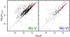 |
Fig. 1 Comparison of our weighted oscillator strengths to those of Reader & Tauheed (2015) for Mo v (left) and of Reader (2010) for Mo vi (right). The larger, red symbols refer to the lines identified in RE 0503−289 (Table A.9). |
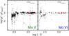 |
Fig. 2 Ratio of our weighted oscillator strengths and those of Reader & Tauheed (2015) for Mo v (left) and of Reader (2010) for Mo vi (right). The wavelength ranges of our FUSE and HST/STIS spectra are marked. The larger, red symbols refer to the lines identified in RE 0503−289 (Table A.9). |
5. The GAVO service TOSS
In the framework of the GAVO project, we developed the new, registered VO service TOSS. It is designed to provide easy access to calculated oscillator strengths and transition probabilities of any kind in VO-compliant format.
Line data is stored in terms of the Spectral Line Data Model (Osuna et al. 2010) and is accessible through a web browser interface, via the Simple Line Access Protocol SLAP (Salgado et al. 2010), and via the Table Access Protocol TAP (Dowler et al. 2010). The browser-based interface offers a web form, which allows conventional queries by wavelength, element, ionisation stage, etc., exporting to various tabular formats and also directly into user programs via SAMP9.
The SLAP interface can be used from specialized programs (“SLAP clients”) like VOSpec (Osuna et al. 2005); this is normally transparent to the user; in a server selector, the service will typically appear under its short name TOSS SLAP.
The TAP interface allows database queries against the line database, including comparisons with user-provided data (“uploads”). In the TAP dialogs of applications like TOPCAT, the user should look for “GAVO DC” or manually enter the access URL10. As the discussion of TAP’s possibilities is beyond the scope of this paper, see on-line examples for TOSS service usage11.
6. Photospheric abundances
To improve the simulation of the background opacity, we included As in our calculations for G191−B2B and RE 0503−289 and determined its abundance from these models (Sect. 6.1). Then, we included Sn for RE 0503−289 (Sect. 6.2) because our new HST/STIS observation provides access to Sn iv lines that are necessary for an abundance analysis. Based on these extended models, we considered Mo and determined its abundances for RE 0503−289 (Sect. 6.3) and G191−B2B (Sect. 6.4).
6.1. G191-B2B and RE 0503-289: Arsenic (Z = 33)
In the FUSE observation of RE 0503−289, Werner et al. (2012b) discovered As vλλ 987.65,1029.48,1051.6,1056.7 Å. For As v, lifetimes were measured with the beam-foil technique (Pinnington et al. 1981). The multiplet f-value (0.78 ± 0.06) of the As v resonance transition was determined with the help of arbitrarily normalized decay curve (ANDC) analyses, which were confirmed by calculations of Fischer (1977), Migdalek & Baylis (1979), and Curtis & Theodosiou (1989). Morton (2000) lists both components in his compilation, λ 987.65 Å (4s 2S1/2–4p 2P , f = 0.528) and λ 1029.48 Å (4s 2S1/2–4p 2P
 , f = 0.253). These were used by Chayer et al. (2015) to determine arsenic mass fractions. They found 6.3 × 10⁻⁸ (6 times solar) and 1.6 × 10⁻⁵ (1450 times solar) in G191−B2B and RE 0503−289, respectively.
As vλλ 1051.6,1056.7 Å belong to the 4d 2D−4f 2F° multiplet (λλ1050.67,1051.64,1055.60,1056.58) but no oscillator strengths have been calculated so far.
We included the TMAD As iv-viii model atom in our model-atmosphere calculations. As vi is the dominant ion in the line-forming region in both stars (Figs. 3 and 4). We reproduced the observed As vλλ 987.65,1029.48 Å line profiles well in the FUSE spectra of G191−B2B and RE 0503−289 at mass fractions of 3.7 × 10⁻⁷ (29 times solar) and 8.3 × 10⁻⁶ (760 times solar), respectively (Fig. 5). Our abundances deviate by factors of 6 and 0.5 for G191−B2B and RE 0503−289, respectively, from those of Chayer et al. (2015), who made an LTE assumption because of lack of atomic data. Both stars are out of the validity domain for LTE modeling (e.g., Rauch 2012), which is corroborated by an inspection of the departure coefficients (ratio of NLTE to LTE occupation numbers) of the five lowest As v levels in our models for G191−B2B and RE 0503−289 that deviate from unity (Fig. 6 and 7, respectively). Therefore, the results of an LTE analysis may be afflicted by a large systematic error.
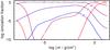 |
Fig. 3 Arsenic ionization fractions in our RE 0503−289 model. m is the column mass, measured from the outer boundary of the model atmosphere. |
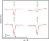 |
Fig. 5 Sections of our FUSE observations of G191−B2B (top row) and RE 0503−289 (bottom row) around As vλ 987.65 Å (left column) and As vλ 1029.48 Å (right column). The thick red and thin green lines show a comparison with theoretical spectra of two models, with and without As, respectively. |
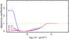 |
Fig. 7 As for Fig. 6, for RE 0503−289. |
Figure 8 shows a comparison of theoretical profiles of As vλλ 987.65,1029.48 Å that are calculated from our NLTE model and an LTE model (calculated by TMAD based on the temperature and density stratification of the NLTE model, LTE occupation numbers of the atomic levels are enforced by an artificial increase of all collisional rates by a factor of 1020). In the case of G191−B2B, the LTE profiles are too strong and, thus, the abundance had to be reduced to 1.0 × 10⁻⁷ to match the observation. For RE 0503−289, they are too weak and, thus, a higher abundance of 1.7 × 10⁻⁵ is needed to reproduce the observation. This may explain, in part, the deviation of our As abundances from those of Chayer et al. (2015).
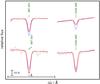 |
Fig. 8 As for Fig. 5, the thick red and dashed blue lines show a comparison with theoretical spectra of NLTE and LTE models, respectively. |
However, a precise abundance analysis by means of NLTE model-atmosphere techniques requires reliable oscillator strengths, not only for the lines employed in the abundance determination, but for the complete model atom that is considered in the model-atmosphere and spectral-energy-distribution calculations. Once these oscillator strengths become available for a large number of As v-vii lines, it will be possible to construct much more complete As model ions and a new determination of the As abundance will be more precise.
6.2. RE 0503-289: Tin (Z = 50)
Rauch et al. (2013) measured the Sn abundance in G191−B2B (3.53 × 10⁻⁷, 37 times solar). They used the lines of the resonance doublet, namely, Sn ivλ 1314.537 Å (5s 2S1/2–5p 2P, f = 0.637) and λ 1437.525 Å (5s 2S1/2–5p 2P, f = 0.240). Their f-values were calculated by Morton (2000) based on energy levels provided by Moore (1958). These lines are visible in our HST/STIS spectrum of RE 0503−289 as well. To determine the Sn abundance, we used the same model atom like Rauch et al. (2013) and reproduced the observed line profiles of both lines (Fig. 9) well at a mass fraction of 2.04 × 10⁻⁴ (about 22 500 times solar). This Sn abundance analysis will also be improved, as soon as reliable transition probabilities for Sn iv-vi are published.
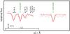 |
Fig. 9 Sections of our HST/STIS observations of RE 0503−289 around Sn ivλ 1314.537 Å (left) and Sn ivλ 1427.525 Å (right). The thick, red and thin, green lines show a comparison with theoretical spectra of two models with and without Sn, respectively. |
6.3. RE 0503-289: Molybdenum
Our RE 0503−289 model (Teff = 70 000 K, log g = 7.5) includes opacities of H, He, C, N, O, Si, P, S, Ca, Sc, Ti, V, Cr, Mn, Fe, Co, Ni, Zn, Ga, Ge, As, Kr, Mo, Xe, and Ba. Figure 10 shows the Mo ionization fractions in this model. Mo vi+vii are the dominating ionization stages in the line-forming region (−4.0 ≲ log m ≲ 0.5). The element abundances are given in Table 2. In general, their uncertainty is about 0.2 dex. This includes the error propagation due to the error ranges of Teff (cf., e.g., Vennes & Lanz 2001), log g, and the background opacity.
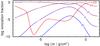 |
Fig. 10 Molybdenum ionization fractions in our RE 0503−289 model. |
Photospheric abundances of RE 0503−289.
Figure 11 shows the relative line strengths (normalized to that of Mo viλ 1038.642 Å) of the Mo lines in the synthetic spectrum of RE 0503−289. We note that these strengths reduce if the spectrum is convolved with a Gaussian to match the instruments’ resolutions (Sect. 2).
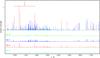 |
Fig. 11 Relative strengths of Mo lines calculated from our stellar-atmosphere model of RE 0503−289. Top graph: Mo iv–vii lines, the four most prominent are Mo vi lines that were identified by Werner et al. (2012b) are marked. Graphs 2 to 5 (from top to bottom): lines of individual Mo iv–vii ions (intensities reduced by a factor of 0.22 compared to the top graph), respectively. |
In the FUSE and HST/STIS observations, we identified 12 Mo v and nine Mo vi lines (Fig. 12). Their strengths were well reproduced at a Mo abundance of 1.88 × 10⁻⁴ (mass fraction), which is 35 400 times the solar value (Grevesse et al. 2015). Many more weak Mo v and Mo vi lines are visible in the synthetic spectrum but they fade in the noise of the presently available observations. The search for the strongest Mo iv and Mo vii lines (Fig. 11) was not successful. This was not unexpected, given the predicted weakness of the lines and the S/N of the data. Figure 13 shows the two strongest Mo vii lines of our model. We note that Ba viiλ 1255.520 Å dominates the observed absorption around λ1255.5 Å (Fig. 13).
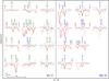 |
Fig. 12 Mo v lines (left panel, marked with their wavelengths from Table A.11 in Å, green) and Mo vi lines (right panel, marked blue, wavelengths from Table A.12) in the FUSE (for lines at λ< 1188 Å) and HST/STIS (λ> 1188 Å) observations of RE 0503−289. The synthetic spectra are convolved with a Gaussian (full width at half maximum = FWHM = 0.06 Å) to simulate the instruments’ resolutions. Other identified photospheric lines are marked in black. The thick red and thin green lines show a comparison with theoretical spectra of two models with and without Mo, respectively. The vertical bar indicates 10% of the continuum flux. |
The identification of Mo lines in the wavelength region λ ≳ 1700 Å was strongly hampered by the lower signal-to-noise (S/N) and resolution (only a fourth of the exposure time and 66% of the resolving power of the spectrum, compared to the region at λ ≲ 1700 Å, see Sect. 2). An example is shown in Fig. 14. Mo vλ 1718.088 Å appears at comparable strengths of other lines that were identified (Fig. 12). However, it is within the noise level of the observation and has to be judged uncertain. Mo viλ 1718.238 Å is weaker but a better observation would allow an identification.
6.4. G191-B2B: Molybdenum
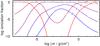
We added Mo into our atmosphere model (Teff = 60 000 K, log g = 7.6) for G191−B2B, which considers H, He, C, N, O, Al, Si, P, S, Ca, Sc, Ti, V, Cr, Mn, Fe, Co, Ni, Zn, Ga, Ge, As, Mo, Sn, and Ba. The abundances are given in Table 3. Mo vi+vii are the dominating ionization fractions in the line-forming region (Fig. 15).
We performed a search for Mo lines in the observed spectra of G191−B2B, analogous to that in Sect. 6.3. However, we did not identify any. Figure 16 shows a comparison of our synthetic spectra to the observations. Since the HST/STIS spectrum of G191−B2B (Sect. 2) is of excellent quality, Mo viλ 1469.168 Å gives a stringent upper abundance limit of 5.3 × 10⁻⁷ by mass (about 100 times solar, Grevesse et al. 2015).
6.5. G191-B2B: Krypton (Z = 36) and Xenon (Z = 54)
For G191−B2B, we have determined a relatively high upper abundance limit (about 100 times solar) for Mo (Sect. 6.4). This is well in agreement with a factor of about 100−1000 between the trans-iron element abundances in RE 0503−289 and G191−B2B. Like Mo, Kr, and Xe exhibit prominent lines in the UV spectra of RE 0503−289, but not in those of G191−B2B. To investigate on their abundances, we individually included Kr and Xe in our G191−B2B models and calculated theoretical profiles for all Kr and Xe lines that were identified in RE 0503−289 (Werner et al. 2012b; Rauch et al. 2015a). An upper Kr abundance limit of 10 times solar (1.09 × 10⁻⁶ by mass) is determined from lines of Kr vi-vii simultaneously (Fig. 17). In the case of Xe, the intersystem lines Xe viiλ 995.51 Å (5s2 1S−5s5p 3P°) and
Xe viiλ 1077.12 Å (5s5p 1P°–5p2 1D) are very strong (Fig. 17) and require an upper Xe abundance limit of solar to fade in the noise of the observation. However, this may be strongly underestimated because of the rudimentary Xe vii model atom presently provided by TMAD. In that, only two Xe vii lines with reliable oscillator strengths are known, namely, 0.245 for Xe viiλ 995.51 Å (Kernahan et al. 1980) and 0.810 for Xe viiλ 1077.12 Å (Biémont et al. 2007). Since, for the calculation of accurate NLTE occupation numbers of the atomic levels of an specific model ion, reliable transition probabilities are mandatory for the complete ion, the Xe vii upper limit is regarded as uncertain. This issue is out of the scope of this paper but will be investigated in detail immediately after new Xe iv-vii transition probabilities become available. However, from the Xe vi lines alone, we achieve an upper limit of 1.7 × 10⁻⁷ (10 times the solar value, Fig. 17).
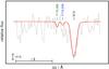 |
Fig. 14 Section of our HST/STIS observations of RE 0503−289 around N ivλ 1718.55 Å. The thick red and thin green lines show a comparison with theoretical spectra of two models with and without Mo, respectively. Mo vλ 1718.088 Å and Mo viλ 1718.238 Å are marked. |
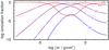 |
Fig. 15 Same as Fig. 10 for G191−B2B. For comparison, the dashed lines show the Mo vi+vii ionization fractions in the RE 0503−289 model. |
7. Impact of diffusion on trans-iron elements
At almost the same log g, RE 0503−289 has a significantly higher Teff compared to that of G191−B2B (Teff = 70 000 K, log g = 7.5 vs. Teff = 60 000 K, log g = 7.6, respectively). Thus, the much stronger enrichment of the trans-iron elements in RE 0503−289 (Fig. 18) may be the result of a more efficient radiative levitation. Therefore, we used the NGRT12 code (Dreizler & Wolff 1999; Schuh et al. 2002) to calculate diffusion models for both stars, using exactly the same model atoms for H, He, C, N, O, Ca, Sc, Ti, V, Cr, Mn, Fe, Co, Ni, Zn, Ga, Ge, As, Kr, Mo, Sn, Xe, and Ba, which were used for our chemically homogeneous TMAP models. For RE 0503−289, H was formally included in the calculation, but its abundance was fixed to 1.0 × 10⁻²⁰. Therefore, its contribution to the background opacity is negligible. Disregarding the fixed H abundance in RE 0503−289, the diffusion models differ only in Teff and log g.
The TMAD model atoms for As and Sn are presently rather rudimentary, especially as only a very few oscillator strengths are known. Restricting the radiative levitation calculation to include transitions with known oscillator strengths thus leads to an unrealistically small effect. We follow Rauch et al. (2013) and add all allowed line transitions in our As and Sn model atoms, using default f-values of 1. Therefore, the results of our diffusion models for these elements should be regarded as preliminary.
Figure 19 shows the calculated depth-dependent abundance profiles for Zn, Ga, Ge, As, Kr, Mo, Sn, Xe, and Ba. All these are strongly overabundant in the line-forming regions (Fig. 19). The predicted abundance profiles suggest abundance enhancements in RE 0503−289 relative to G191−B2B. This is qualitatively in agreement with the abundance patterns in Fig. 18, which were determined from our static TMAP models. However, whether it is possible to reach 2−3 dex should be demonstrated with advanced line-profile calculations in diffusive equilibrium. These would provide stringent constraints for suggested weak stellar winds (Chayer et al. 2005) and thin convective zones at the stellar surface (Chayer et al. 2015), which might impact the interplay of radiative levitation and gravitational settling.
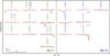 |
Fig. 16 Like Fig. 12 for G191−B2B. The thick red and thin blue spectra are calculated from models with photospheric Mo abundances of 5.3 × 10⁻⁶ and 5.3 × 10⁻⁷ (mass fractions, about 1000 and 100 times the solar value), respectively. |
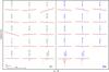 |
Fig. 17 Theoretical line profiles of Kr (left panel, 14 Kr vi lines and 1 Kr vii line) and Xe (right panel, 12 Xe vi and 2 Xe vii lines) compared to the observations of G191−B2B. The spectra are calculated from models with photospheric abundances (mass fractions) of Kr: 1.1 × 10⁻⁵ (thick red, 100 times solar) and 1.1 × 10⁻⁶ (thin blue, 10 times solar) and of Xe: 1.7 × 10⁻⁶ (dashed black, 100 times solar), 1.7 × 10⁻⁷ (thick red, 10 times solar), and 1.7 × 10⁻⁸ (thin blue, solar). |
8. Results and conclusions
With our NLTE model-atmosphere package TMAP, we calculated new models for the DO-type white dwarf RE 0503−289 with molybdenum in addition. The Mo model atoms were constructed with newly calculated Mo iv–vii oscillator strengths. We have unambiguously identified 12 Mo v and nine Mo vi lines in the observed high-resolution UV spectra of RE 0503−289. The Mo v/Mo vi ionization equilibrium is well reproduced (Fig. 12). We determined a photospheric abundance of log Mo = −3.73 ± 0.2 (mass fraction 1.2−3.0 × 10⁻⁴, 22 500−56 400 times the solar abundance). In addition, we determined the arsenic and tin abundances and derived log As = −5.08 ± 0.2 (0.5−1.3 × 10⁻⁵, about 300−1200 times solar) and log Sn = −3.69 ± 0.2 (1.3−3.2 × 10⁻⁴, about 14 300−35 200 times solar). These highly supersolar As, Mo, and Sn abundances agree well with the high abundances of other trans-iron elements in RE 0503−289 (Fig. 18).
G191−B2B does not exhibit Kr, Mo, and Xe lines in its UV spectrum. We investigated the strongest lines in the model and found upper limits for the abundances of Kr (1.1 × 10⁻⁶, 10 times solar), Mo (5.3 × 10⁻⁷, 100 times solar), and Xe (1.7 × 10⁻⁷, 10 times solar). Whether radiative levitation yields abundances of these elements that are consistent with observations should be demonstrated with advanced line-profile calculations in diffusive equilibrium, as depicted in Fig. 19. In addition, we determined the arsenic abundance and derived log As = −6.43 ± 0.2 (2.3−5.9 × 10⁻⁷, about 21−53 times solar).
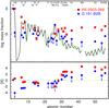 |
Fig. 18 Solar abundances (Asplund et al. 2009; Scott et al. 2015b,a; Grevesse et al. 2015, thick line; the dashed green lines connect the elements with even and with odd atomic number) compared with the determined photospheric abundances of G191−B2B (blue circles, Rauch et al. 2013) and RE 0503−289 (red squares, Dreizler & Werner 1996; Werner et al. 2012b; Rauch et al. 2013, 2014a,b, 2015a,b, and this work). Top panel: abundances given as logarithmic mass fractions. Arrows indicate upper limits. Bottom panel: abundance ratios to respective solar values, [X] denotes log (fraction/solar fraction) of species X. The dashed green line indicates solar abundances. |
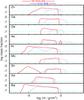 |
Fig. 19 Abundance profiles in our diffusion models for G191−B2B (thin blue) and RE 0503−289 (thick red). The dashed, horizontal lines indicate solar abundance values. The formation regions of UV lines in both models are indicated at the top. |
The computation of reliable transition probabilities for Mo iv–vii was a prerequisite for the identification of Mo lines and the subsequent abundance determination. The hitherto known abundance pattern of RE 0503−289 (Fig. 18) indicates that other yet unidentified species should be detectable. Therefore, the precise evaluation of their laboratory spectra, i.e., the measurement of line wavelengths and strengths, as well as the determination of level energies and the subsequent calculation of transition probabilities are absolutely essential.
The example of the arsenic abundance determination (Sect. 6.1) had demonstrated that state-of-the-art NLTE stellar-atmosphere models are mandatory for the precise spectral analysis of hot stars.
Available at http://www.stsci.edu/hst/observatory/cdbs/calspec.html
Non-local thermodynamic equilibrium.
GFxxyy.GAM, GFxxyy.LIN, and GFxxyy.POS files with xx = element number, yy = element charge, http://kurucz.harvard.edu/atoms.html
The Simple Application Messaging Protocol is a VO-defined standard protocol facilitating seamless and fast data exchange on user desktops.
New Generation Radiative Transport.
Acknowledgments
T.R. and D H. are supported by the German Aerospace Center (DLR, grants 05 OR 1402 and 50 OR 1501, respectively). The GAVO project had been supported by the Federal Ministry of Education and Research (BMBF) at Tübingen (05 AC 6 VTB, 05 AC 11 VTB) and is funded at Heidelberg (05 AC 11 VH3). Financial support from the Belgian FRS-FNRS is also acknowledged. P.Q. is research director of this organization. We thank our referee, Stéphane Vennes, for constructive criticism. Some of the data presented in this paper were obtained from the Mikulski Archive for Space Telescopes (MAST). STScI is operated by the Association of Universities for Research in Astronomy, Inc., under NASA contract NAS5-26555. Support for MAST for non-HST data is provided by the NASA Office of Space Science via grant NNX09AF08G and by other grants and contracts. This research has made use of NASA’s Astrophysics Data System and the SIMBAD database, operated at CDS, Strasbourg, France. The TOSS service (http://dc.g-vo.org/TOSS) that provides weighted oscillator strengths and transition probabilities was constructed as part of the activities of the German Astrophysical Virtual Observatory.
References
- Asplund, M., Grevesse, N., Sauval, A. J., & Scott, P. 2009, ARA&A, 47, 481 [NASA ADS] [CrossRef] [Google Scholar]
- Biémont, É., Clar, M., Fivet, V., et al. 2007, Eur. Phys. J. D, 44, 23 [NASA ADS] [CrossRef] [EDP Sciences] [Google Scholar]
- Cabeza, M. I., Iglesias, L., Rico, F. R., & Kaufman, V. 1989, Phys. Scr, 40, 457 [NASA ADS] [CrossRef] [Google Scholar]
- Chayer, P., Vennes, S., Dupuis, J., & Kruk, J. W. 2005, ApJ, 630, L169 [NASA ADS] [CrossRef] [Google Scholar]
- Chayer, P., Dupuis, J., & Kruk, J. W. 2015, in 19th European Workshop on White Dwarfs, eds. P. Dufour, P. Bergeron, & G. Fontaine, ASP Conf. Ser., 493, 3 [Google Scholar]
- Cowan, R. D. 1981, The theory of atomic structure and spectra (Berkeley, CA: University of California Press) [Google Scholar]
- Cowley, C. R. 1970, The theory of stellar spectra (New York: Gordon & Breach) [Google Scholar]
- Cowley, C. R. 1971, The Observatory, 91, 139 [NASA ADS] [Google Scholar]
- Curtis, L. J., & Theodosiou, C. E. 1989, Phys. Rev. A, 39, 605 [NASA ADS] [CrossRef] [PubMed] [Google Scholar]
- Dowler, P., Rixon, G., & Tody, D. 2010, Table Access Protocol Version 1.0, IVOA Recommendation [Google Scholar]
- Dreizler, S., & Werner, K. 1996, A&A, 314, 217 [NASA ADS] [Google Scholar]
- Dreizler, S., & Wolff, B. 1999, A&A, 348, 189 [NASA ADS] [Google Scholar]
- Fischer, C. F. 1977, J. Phys. B, 10, 1241 [Google Scholar]
- Fraga, S., Karwowski, J., & Saxena, K. M. S. 1976, Handbook of Atomic Data (Amsterdam: Elsevier) [Google Scholar]
- Grevesse, N., Scott, P., Asplund, M., & Sauval, A. J. 2015, A&A, 573, A27 [NASA ADS] [CrossRef] [EDP Sciences] [Google Scholar]
- Hubeny, I., Hummer, D. G., & Lanz, T. 1994, A&A, 282, 151 [NASA ADS] [Google Scholar]
- Hummer, D. G., & Mihalas, D. 1988, ApJ, 331, 794 [NASA ADS] [CrossRef] [Google Scholar]
- Johnson, W. R., Kolb, D., & Huang, K.-N. 1983, Atomic Data and Nuclear Data Tables, 28, 333 [Google Scholar]
- Kernahan, J. A., Pinnington, E. H., O’Neill, J. A., Bahr, J. L., & Donnelly, K. E. 1980, J. Opt. Soc. Am., 70, 1126 [NASA ADS] [CrossRef] [Google Scholar]
- McCook, G. P., & Sion, E. M. 1999a, ApJS, 121, 1 [NASA ADS] [CrossRef] [Google Scholar]
- McCook, G. P., & Sion, E. M. 1999b, VizieR Online Data Catalog: III/210 [Google Scholar]
- Migdalek, J., & Baylis, W. E. 1979, J. Phys. B, 12, 1113 [NASA ADS] [CrossRef] [Google Scholar]
- Moore, C. E. 1958, Atomic Energy Levels as Derived from the Analysis of Optical Spectra Molybdenum through Lanthanum and Hafnium through Actinium (NIST) [Google Scholar]
- Morton, D. C. 2000, ApJS, 130, 403 [NASA ADS] [CrossRef] [MathSciNet] [Google Scholar]
- Osuna, P., Barbarisi, I., Salgado, J., & Arviset, C. 2005, in Astronomical Data Analysis Software and Systems XIV, eds. P. Shopbell, M. Britton, & R. Ebert, ASP Conf. Ser., 347, 198 [Google Scholar]
- Osuna, P., Guainazzi, M., Salgado, J., Dubernet, M.-L., & Roueff, E. 2010, Simple Spectral Lines Data Model, IVOA Recommendation 2 Dec [Google Scholar]
- Pinnington, E. H., Bahr, J. L., Kernahan, J. A., & Irwin, D. J. G. 1981, J. Phys. B, 14, 1291 [Google Scholar]
- Quinet, P., Palmeri, P., Biémont, E., et al. 1999, MNRAS, 307, 934 [NASA ADS] [CrossRef] [EDP Sciences] [Google Scholar]
- Quinet, P., Palmeri, P., Biémont, E., et al. 2002, J. Alloys Comp., 344, 255 [CrossRef] [Google Scholar]
- Rauch, T. 2012, ArXiv e-prints [arXiv:1210.7636] [Google Scholar]
- Rauch, T., & Deetjen, J. L. 2003, in Stellar Atmosphere Modeling, eds. I. Hubeny, D. Mihalas, & K. Werner, ASP Conf. Ser., 288, 103 [Google Scholar]
- Rauch, T., Werner, K., Biémont, É., Quinet, P., & Kruk, J. W. 2012, A&A, 546, A55 [NASA ADS] [CrossRef] [EDP Sciences] [Google Scholar]
- Rauch, T., Werner, K., Bohlin, R., & Kruk, J. W. 2013, A&A, 560, A106 [NASA ADS] [CrossRef] [EDP Sciences] [Google Scholar]
- Rauch, T., Werner, K., Quinet, P., & Kruk, J. W. 2014a, A&A, 564, A41 [NASA ADS] [CrossRef] [EDP Sciences] [Google Scholar]
- Rauch, T., Werner, K., Quinet, P., & Kruk, J. W. 2014b, A&A, 566, A10 [NASA ADS] [CrossRef] [EDP Sciences] [Google Scholar]
- Rauch, T., Hoyer, D., Quinet, P., Gallardo, M., & Raineri, M. 2015a, A&A, 577, A88 [NASA ADS] [CrossRef] [EDP Sciences] [Google Scholar]
- Rauch, T., Werner, K., Quinet, P., & Kruk, J. W. 2015b, A&A, 577, A6 [NASA ADS] [CrossRef] [EDP Sciences] [Google Scholar]
- Reader, J. 2010, J. Phys. B, 43, 074024 [NASA ADS] [CrossRef] [Google Scholar]
- Reader, J., & Tauheed, A. 2015, J. Phys B, 48, 144001 [NASA ADS] [CrossRef] [Google Scholar]
- Salgado, J., Osuna, P., Guainazzi, M., et al. 2010, Simple Line Access Protocol, IVOA http://www.ivoa.net/documents/SLAP/ [Google Scholar]
- Schuh, S. L., Dreizler, S., & Wolff, B. 2002, A&A, 382, 164 [NASA ADS] [CrossRef] [EDP Sciences] [Google Scholar]
- Scott, P., Asplund, M., Grevesse, N., Bergemann, M., & Sauval, A. J. 2015a, A&A, 573, A26 [NASA ADS] [CrossRef] [EDP Sciences] [Google Scholar]
- Scott, P., Grevesse, N., Asplund, M., et al. 2015b, A&A, 573, A25 [NASA ADS] [CrossRef] [EDP Sciences] [Google Scholar]
- Shirai, T., Sugar, J., Musgrove, A., & Wiese, W. L. 2000, Spectral Data for Highly Ionized Atoms: Ti, V, Cr, Mn, Fe, Co, Ni, Cu, Kr, and Mo (AIP) [Google Scholar]
- Sugar, J., & Musgrove, A. 1988, J. Phys. Chem. Ref. Data, 17, 155 [Google Scholar]
- Vennes, S., & Lanz, T. 2001, ApJ, 553, 399 [NASA ADS] [CrossRef] [Google Scholar]
- Werner, K., Deetjen, J. L., Dreizler, S., et al. 2003, in Stellar Atmosphere Modeling, eds. I. Hubeny, D. Mihalas, & K. Werner, ASP Conf. Ser., 288, 31 [Google Scholar]
- Werner, K., Dreizler, S., & Rauch, T. 2012a, TMAP: Tübingen NLTE Model-Atmosphere Package (Astrophysics Source Code Library) [Google Scholar]
- Werner, K., Rauch, T., Ringat, E., & Kruk, J. W. 2012b, ApJ, 753, L7 [NASA ADS] [CrossRef] [Google Scholar]
Appendix A: Additional tables
Radial parameters (in cm-1) adopted for the calculations in Mo iv.
Radial parameters (in cm-1) adopted for the calculations in Mo v.
Radial parameters (in cm-1) adopted for the calculations in Mo vi.
Radial parameters (in cm-1) adopted for the calculations in Mo vii.
Comparison between available experimental and calculated energy levels in Mo iv. Energies are given in cm-1.
Comparison between available experimental and calculated energy levels in Mo v. Energies are given in cm-1.
Comparison between available experimental and calculated energy levels in Mo vi. Energies are given in cm-1.
Comparison between available experimental and calculated energy levels in Mo vii. Energies are given in cm-1.
Comparison of wavelengths and log gf values of the identified Mo v and Mo vi lines to literature values.
All Tables
Statistics of Mo iv - vii atomic levels and line transitions from Tables A.10–A.13, respectively.
Comparison between available experimental and calculated energy levels in Mo iv. Energies are given in cm-1.
Comparison between available experimental and calculated energy levels in Mo v. Energies are given in cm-1.
Comparison between available experimental and calculated energy levels in Mo vi. Energies are given in cm-1.
Comparison between available experimental and calculated energy levels in Mo vii. Energies are given in cm-1.
Comparison of wavelengths and log gf values of the identified Mo v and Mo vi lines to literature values.
All Figures
|
Fig. 1 Comparison of our weighted oscillator strengths to those of Reader & Tauheed (2015) for Mo v (left) and of Reader (2010) for Mo vi (right). The larger, red symbols refer to the lines identified in RE 0503−289 (Table A.9). |
| In the text | |
|
Fig. 2 Ratio of our weighted oscillator strengths and those of Reader & Tauheed (2015) for Mo v (left) and of Reader (2010) for Mo vi (right). The wavelength ranges of our FUSE and HST/STIS spectra are marked. The larger, red symbols refer to the lines identified in RE 0503−289 (Table A.9). |
| In the text | |
|
Fig. 3 Arsenic ionization fractions in our RE 0503−289 model. m is the column mass, measured from the outer boundary of the model atmosphere. |
| In the text | |
|
Fig. 5 Sections of our FUSE observations of G191−B2B (top row) and RE 0503−289 (bottom row) around As vλ 987.65 Å (left column) and As vλ 1029.48 Å (right column). The thick red and thin green lines show a comparison with theoretical spectra of two models, with and without As, respectively. |
| In the text | |
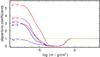 |
Fig. 6 Departure coefficients of the five lowest As v levels in the model for G191−B2B. |
| In the text | |
|
Fig. 7 As for Fig. 6, for RE 0503−289. |
| In the text | |
|
Fig. 8 As for Fig. 5, the thick red and dashed blue lines show a comparison with theoretical spectra of NLTE and LTE models, respectively. |
| In the text | |
|
Fig. 9 Sections of our HST/STIS observations of RE 0503−289 around Sn ivλ 1314.537 Å (left) and Sn ivλ 1427.525 Å (right). The thick, red and thin, green lines show a comparison with theoretical spectra of two models with and without Sn, respectively. |
| In the text | |
|
Fig. 10 Molybdenum ionization fractions in our RE 0503−289 model. |
| In the text | |
|
Fig. 11 Relative strengths of Mo lines calculated from our stellar-atmosphere model of RE 0503−289. Top graph: Mo iv–vii lines, the four most prominent are Mo vi lines that were identified by Werner et al. (2012b) are marked. Graphs 2 to 5 (from top to bottom): lines of individual Mo iv–vii ions (intensities reduced by a factor of 0.22 compared to the top graph), respectively. |
| In the text | |
|
Fig. 12 Mo v lines (left panel, marked with their wavelengths from Table A.11 in Å, green) and Mo vi lines (right panel, marked blue, wavelengths from Table A.12) in the FUSE (for lines at λ< 1188 Å) and HST/STIS (λ> 1188 Å) observations of RE 0503−289. The synthetic spectra are convolved with a Gaussian (full width at half maximum = FWHM = 0.06 Å) to simulate the instruments’ resolutions. Other identified photospheric lines are marked in black. The thick red and thin green lines show a comparison with theoretical spectra of two models with and without Mo, respectively. The vertical bar indicates 10% of the continuum flux. |
| In the text | |
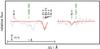 |
Fig. 13 Same as Fig. 12, for two Mo vii lines. |
| In the text | |
|
Fig. 14 Section of our HST/STIS observations of RE 0503−289 around N ivλ 1718.55 Å. The thick red and thin green lines show a comparison with theoretical spectra of two models with and without Mo, respectively. Mo vλ 1718.088 Å and Mo viλ 1718.238 Å are marked. |
| In the text | |
|
Fig. 15 Same as Fig. 10 for G191−B2B. For comparison, the dashed lines show the Mo vi+vii ionization fractions in the RE 0503−289 model. |
| In the text | |
|
Fig. 16 Like Fig. 12 for G191−B2B. The thick red and thin blue spectra are calculated from models with photospheric Mo abundances of 5.3 × 10⁻⁶ and 5.3 × 10⁻⁷ (mass fractions, about 1000 and 100 times the solar value), respectively. |
| In the text | |
|
Fig. 17 Theoretical line profiles of Kr (left panel, 14 Kr vi lines and 1 Kr vii line) and Xe (right panel, 12 Xe vi and 2 Xe vii lines) compared to the observations of G191−B2B. The spectra are calculated from models with photospheric abundances (mass fractions) of Kr: 1.1 × 10⁻⁵ (thick red, 100 times solar) and 1.1 × 10⁻⁶ (thin blue, 10 times solar) and of Xe: 1.7 × 10⁻⁶ (dashed black, 100 times solar), 1.7 × 10⁻⁷ (thick red, 10 times solar), and 1.7 × 10⁻⁸ (thin blue, solar). |
| In the text | |
|
Fig. 18 Solar abundances (Asplund et al. 2009; Scott et al. 2015b,a; Grevesse et al. 2015, thick line; the dashed green lines connect the elements with even and with odd atomic number) compared with the determined photospheric abundances of G191−B2B (blue circles, Rauch et al. 2013) and RE 0503−289 (red squares, Dreizler & Werner 1996; Werner et al. 2012b; Rauch et al. 2013, 2014a,b, 2015a,b, and this work). Top panel: abundances given as logarithmic mass fractions. Arrows indicate upper limits. Bottom panel: abundance ratios to respective solar values, [X] denotes log (fraction/solar fraction) of species X. The dashed green line indicates solar abundances. |
| In the text | |
|
Fig. 19 Abundance profiles in our diffusion models for G191−B2B (thin blue) and RE 0503−289 (thick red). The dashed, horizontal lines indicate solar abundance values. The formation regions of UV lines in both models are indicated at the top. |
| In the text | |
Current usage metrics show cumulative count of Article Views (full-text article views including HTML views, PDF and ePub downloads, according to the available data) and Abstracts Views on Vision4Press platform.
Data correspond to usage on the plateform after 2015. The current usage metrics is available 48-96 hours after online publication and is updated daily on week days.
Initial download of the metrics may take a while.