| Issue |
A&A
Volume 587, March 2016
|
|
|---|---|---|
| Article Number | A75 | |
| Number of page(s) | 17 | |
| Section | Interstellar and circumstellar matter | |
| DOI | https://doi.org/10.1051/0004-6361/201526532 | |
| Published online | 19 February 2016 | |
Proper motions of embedded protostellar jets in Serpens⋆
1
Nordic Optical Telescope, Rambla José Ana Fernández Pérez, 7,
38711
Breña Baja,
Spain
e-mail:
This email address is being protected from spambots. You need JavaScript enabled to view it.
2
Tartu Observatory, 61602
Tõravere,
Estonia
e-mail:
This email address is being protected from spambots. You need JavaScript enabled to view it.
3
Institute of Physics, University of Tartu,
Ravila 14c, 50411
Tartu,
Estonia
4 SOFIA Science Center, NASA Ames Research Center, 94035
Moffett Field, USA
e-mail:
This email address is being protected from spambots. You need JavaScript enabled to view it.
5
Deutsches SOFIA Institut (DSI), University of
Stuttgart, 70569
Stuttgart,
Germany
6
Institute of Astronomy, University of Latvia,
Raina bulv. 19, Riga,
LV
1586,
Latvia
7
School of Maths & Physics, University of
Tasmania, 7001
Hobart,
Australia
e-mail:
This email address is being protected from spambots. You need JavaScript enabled to view it.
8
Niels Bohr Institute, University of Copenhagen,
Juliane Maries Vej 30,
2100
Copenhagen,
Denmark
Received: 14 May 2015
Accepted: 18 December 2015
Abstract
Aims. We determine the proper motion of protostellar jets around Class 0 and Class I sources in an active star forming region in Serpens.
Methods. Multi-epoch deep images in the 2.122 μm line of molecular hydrogen, v = 1−0 S(1), obtained with the near-infrared instrument NOTCam on a timescale of 10 years, are used to determine the proper motion of knots and jets. K-band spectroscopy of the brighter knots is used to supply radial velocities, estimate extinction, excitation temperature, and H2 column densities towards these knots.
Results. We measure the proper motion of 31 knots on different timescales (2, 4, 6, 8, and 10 years). The typical tangential velocity is around 50 km s-1 for the 10-year baseline, but for shorter timescales, a maximum tangential velocity up to 300 km s-1 is found for a few knots. Based on morphology, velocity information, and the locations of known protostars, we argue for the existence of at least three partly overlapping and deeply embedded flows, one Class 0 flow and two Class I flows. The multi-epoch proper motion results indicate time-variable velocities of the knots, for the first time directly measured for a Class 0 jet. We find in general higher velocities for the Class 0 jet than for the two Class I jets. While the bolometric luminosites of the three driving sources are about equal, the derived mass flow rate Ṁout is two orders of magnitude higher in the Class 0 flow than in the two Class I flows.
Key words: stars: formation / ISM: jets and outflows / Herbig-Haro objects / ISM: kinematics and dynamics
Based on observations made with the Nordic Optical Telescope, operated on the island of La Palma jointly by Denmark, Finland, Iceland, Norway, and Sweden, in the Spanish Observatorio del Roque de los Muchachos of the Instituto de Astrofisica de Canarias.
© ESO, 2016
1. Introduction
Protostellar jets are spectacular manifestations of the birth of a star. Supersonic and collimated jets drive bipolar outflows of molecular gas, removing angular momentum from and allowing accretion onto the protostar. The origin of the jets is poorly understood, but a tight relation between the accretion disk and the jet is evident in magneto-hydro-dynamic models. For a recent review of jets and outflows, see Frank et al. (2014). The power carried by the jet is expected to be proportional to the accretion luminosity of the central star, suggesting that protostellar jets from the youngest protostars have higher velocities. As shown by Bontemps et al. (1996), the youngest Class 0 sources (ages from a few 103 to a few 104 yr) have more energetic CO outflows than the more evolved Class I protostars. Studies of shocked molecular hydrogen in the jets have shown an empirical relation between the H2 jet luminosity and the bolometric luminosity of the driving source, but found no clear distinction between Class 0 and Class I sources (Caratti o Garatti et al. 2006).
Plasma is ejected in the form of a jet that interacts with the circumstellar medium via radiative shocks, giving rise to observable emission in various lines over a broad spectral range (Reipurth & Bally 2001; Bacciotti et al. 2011). The near-infrared emission from such shocks is mainly in lines of [Fe II] and the ro-vibrational lines of molecular hydrogen. The observed features of the latter are referred to as molecular hydrogen emission-line objects (MHOs). In particular, the v = 1−0 S(1) H2 line at 2.122 μm is a good tracer of shock excited emission in low-velocity shocks, and the 2 μm region suffers less from extinction than optical lines and makes it possible to observe the most embedded flows, which potentially are the very youngest jets.
Protostellar jets are often complex morphological structures composed of a multitude of knots and features, and the school-book example of a symmetric bi-polar jet is rarely observed. In regions of dense star formation, one frequently finds asymmetric flows, jets without counter jets, variable ejection, colliding knots, precession, or two jets that are interacting. Mapping the kinematics of the individual knots will facilitate identification of whole entities of jets and make it possible to separate individual flows in crowded regions. This is required for studying the kinematic and physical properties of the jets and their driving sources.
Two-epoch proper motions will give the average tangential velocities between the two epochs, while multi-epoch imaging will allow us to investigate how velocities may vary. Recent multi-epoch (>2 epochs) measurements in the optical, as well as the near-IR of nearby jets in Taurus and Chamaeleon, have revealed time-variable proper motions and even interaction among knots (Bonito et al. 2008; Caratti o Garatti et al. 2009). To determine the velocities of protostellar jets, we need to identify the individual flows and their driving sources. To do this we need both proper motion and radial velocity information.
In this paper we study the dynamics of the individual knots of embedded protostellar jets in the Serpens NH3 cloud, also referred to as the Serpens/G3-G6 region or Serpens Cluster B (see Eiroa et al. 2008, for a review of the region). These jets were first presented in Djupvik et al. (2006), along with new protostar candidates discovered from a near-IR, mid-IR, submm, and radio study of the region. Based on morphology alone, we tentatively identified the driving sources to be the new Class 0 candidate MMS3 for the N-S oriented jet, and a double Class I for the NE-SW-oriented jet. MMS3 was confirmed by Enoch et al. (2009) in their extensive protostar survey (where it is named Ser-emb-1) to be an early Class 0 of very low temperature. While being presumably the youngest protostar in Serpens, it has already developed a protostellar disk (Enoch et al. 2011). Studying these jets allows for a comparison between Class 0 and Class I jets in the same region.
The large cloud extinction to this embedded cluster means that these jets are not detected in the optical. No extended emission is found in deep Hα imaging except for the faint Herbig-Haro object HH 476, discovered in an optical [SII] survey by Ziener & Eislöffel (1999), and for some emission around the association of bright TTauri stars named Serpens/G3-G6 (Cohen & Kuhi 1979).
We obtained deep H2 line imaging in four epochs over ten years. The first epoch of data (2003) was already published in Djupvik et al. (2006), and the second epoch (2009) was taken during the Nordic-Baltic Summer School in Turku, Finland1. Preliminary results, carried out as a student project during the course showed that proper motions indeed could be measured between 2003 and 2009. The data is again reduced here, and in addition, we obtained two more epochs (2011 and 2013), as well as K-band spectroscopy of selected knots, all obtained with NOTCam at the Nordic Optical Telescope (Djupvik & Andersen 2010).
Section 2 describes the target field, observations, and data reduction; Sect. 3 presents the proper motion, fluxes, and radial velocity measurements of the knots, as well as the identification of three distinct flows and their velocities; Sect. 4 describes the derivation of physical parameters for the three flows; and Sect. 5 gives our summary and conclusions.
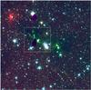 |
Fig. 1 Overview of the Serpens/G3-G6 region (also called Serpens Cluster B and the Serpens NH3 cloud) as seen by IRAC/Spitzer in 3.6 μm (blue), 4.5 μm (green), and 8 μm (red). N up, E left. Total FOV ≈ 15′ × 15′. The jets are mainly enhanced in the 4.5 μm band. The ≈4′ field monitored with NOTCam for proper motions is marked white and shown in Fig. 2. The white arrows point to two bow-shock shaped features outside our monitored field to the N and NE and two jet-like features in the SW region. |
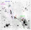 |
Fig. 2 Deep H2 + continuum (2.122 μm) narrowband NOTCam image of the ≈4′ field observed in this multi-epoch study. N up, E left. Naming of jet structures according to the MHO Catalogue is sketched: MHO 2233 (magenta), MHO 2234 (blue), and MHO 2235 (green). The previously known HH 476 is labelled. Red circles show the positions of Class 0 and Class I protostars, the ID number according to designations by Enoch et al. (2009); for instance, 1 refers to the Class 0 source Ser-emb-1, which is named MMS3 in Djupvik et al. (2006). Only a few knots are identified with letters here, and the majority are identified in zoomed-in regions in the following figures. |
2. Target field, observations, and data reductions
2.1. Target field
The Spitzer/IRAC image in Fig. 1 showing the 3.6 μm (blue), 4.5 μm (green), and 8 μm (red) bands gives an overview of the Serpens NH3 region, also called Serpens Cluster B. It is centred on a group of four optically visible and very bright TTauri stars Ser/G3-G6 (Cohen & Kuhi 1979). Two NH3 cores are located to either side, one to the NE and another to the SW, where active star formation takes place and a number of Class 0 and Class I objects are found (Djupvik et al. 2006; Harvey et al. 2006, 2007). The multi-epoch H2 line imaging with NOTCam was obtained in the region outlined by the white box. The jets stand out in the 4.5 μm band emission (green), and apparently they extend beyond the field covered by NOTCam. In Fig. 2 the jets are outlined by the H2 line emission at 2.122 μm. With a narrow-band continuum image centred at 2.087 μm obtained in 2003 the line emission knots were easily distinguished from the continuum (Djupvik et al. 2006). In the MHOs catalogue (Davis et al. 2010), the objects studied in this paper are numbered MHO 2233, MHO 2234, and MHO 2235, with their positions sketched in Fig. 2. Judging from the Spitzer image, it seems that MHO 2233 extends further to the NE, and possibly MHO 2235 to the SW. MHO 2234 extends further to the N, and our 2009 observations confirm 2.122 μm emission in the northernmost bow-shaped feature seen in the IRAC image in Fig. 1, but we have only one epoch of data for it.
Each of the MHO objects are composed of a number of smaller knots, which we identified and named according to the guidelines established in Davis et al. (2010). It is not clear from the 2D morphology, however, which knot belongs to which jet and how many jets there are. Based on proper motions and radial velocities, we show in the following that we find three jets driven by three protostars.
2.2. Imaging
The Nordic Optical Telescope’s near-IR Camera/Spectrograph, NOTCam2, was used to obtain deep multi-epoch narrow-band images in the H2v = 1−0 S(1) line at 2.122 μm (NOT filter #218) to measure proper motions. Four epochs, hereafter referred to as ep1, ep2, ep3, and ep4, are sampled in the years 2003, 2009, 2011, and 2013. The four deep images were obtained with the same instrument, but ep1 was imaged with the NOTCam engineering grade array, while the science array was used for the other three epochs. The wide-field camera of NOTCam has a pixel scale of 0.234′′/pix and a 4′ × 4′ field of view. The deep imaging of the extended emission was mostly performed in beam-switch mode to correctly estimate the sky. In these cases the template NOTCam observing script “notcam.beamswitch” was used to obtain a nine-point grid with small-step dithering both ON target and in the OFF field, going alternatingly between the ON and OFF regions. The OFF field was chosen either to the E, the W, or the N of the central field, the W field being the optimal choice, since it contained no bright disturbing stars whose persistency would affect the background estimate. In the N field we found an additional bow-shaped feature emission line object in 2009. In the 2003 epoch no beamswitch was applied, only small-step dithering around the target field. All narrow-band images were obtained with the ramp-sampling readout mode, where the detector is read a number of times during the integration, typically using 60 s integrations with ten equally spaced readouts. A linear regression analysis is performed pixel by pixel through all reads to obtain the final image.
Table 1 lists the various observations and filters used. The filter ID numbers are according to the internal NOT ID numbers, where 218 refers to the filter centred on the v = 1−0 S(1) line at 2.122 μm, while 210 and 230 refer to narrow-band filters representing the continuum emission at 2.267 and 2.087 μm, respectively. For all filters, differential twilight flats were obtained every night. For flux calibration, two standard star fields were observed before and after the target on the photometric night of May 25, 2013, our reference epoch.
Observing log for NOTCam imaging used in this paper.
The images were reduced using IRAF3 and a set of scripts in an external IRAF package notcam.cl v2.6, made for NOTCam image reductions. All individual raw images were corrected for zero-valued bad pixels and hot pixels by interpolation and then divided by the master flats obtained from typically eight differential twilight flats per filter per night. By using differential flats, the thermal and dark emission is eliminated from the flats. The individual target frames were then sky-subtracted using the off fields obtained in beam-switch mode or the dithered target images themselves. After this step all individual images were corrected for the internal camera distortion. For data from 2009 and onwards we used the distortion model for the KS-band available on the NOTCam calibration web page. For the 2003 data set, a different distortion model was developed based on data from the same night. After distortion correction, all dithered images were registered and combined to form one deep image per epoch.
For flux calibration we used the zeropoint offset between the KS and the H2 line filter (#218) found from eight standard stars in photometric conditions in epoch 4 to be 2.56 ± 0.01 mag, giving a zeropoint for the H2 line filter of 19.94 mag (for 1 ADU/s, Vega magnitudes). Assuming the standards have equal flux at 2.12 and 2.14 (KS) μm, we used the relation for a zeroth magnitude star at 2.121 μm: Fλ = 4.57 × 10⁻¹⁰ W m-2μm-1 (Tokunaga & Vacca 2005), and the FWHM of the filter (0.032 μm), to arrive at a flux conversion of 1.54 × 10⁻¹⁶ erg s-1 cm-2 for 1 ADU/s. The standard deviation of the background in the 2350 s deep image of epoch 4 is 1.5 × 10⁻¹⁶ erg s-1 cm-2 arcsec-2, and the brightest knot, MHO 2235-B, peaks at 1.65 × 10⁻¹⁴ erg s-1 cm-2 arcsec-2.
 |
Fig. 3 Relative position accuracy between epochs checked on stars after the final registration (panels ΔX and ΔY) and flux matching accuracy checked after seeing and flux matching (lower panels). The ΔX and ΔY values are the offsets in X and Y (in pixels) between the measured epoch and the reference epoch (i.e. epoch 4). Epoch 1 is shown to the left, epoch 2 in the centre, and epoch 3 to the right, all plotted with respect to reference X-pixel. In the lower panels we show the flux ratio for the same stars. Black dots indicate all stars, red crosses show stars rejected due to large FWHM and/or high flux ratio, and blue circles indicate stars used for the accuracy calculations. |
In addition, we obtained broad-band JHKs images to illustrate the extinction in the region, with the filters and exposure times listed in Table 1. We also used archive Spitzer data to complement our near-IR imaging with the mid-IR bands of IRAC (Fazio et al. 2004). An RGB colour-coded IRAC image using the 3.6 μm (blue), the 4.5 μm (green), and the 8 μm (red) bands is presented in Fig. 1. The jet clearly stands out in green by enhancing the cuts for the emission in the 4.5 μm band, a wavelength region with many H2 lines. Central parts of both jets have masked out areas in both the 3.6 and 4.5 μm bands. The IRAC imaging was obtained in 2004.
2.3. Spectroscopy
K-band spectroscopy was obtained with NOTCam on October 12, 2011 and March 16 and 17, 2014, in most cases including several knots in the slit for each pointing. The instrument setup was grism #1, the 128 μm slit (a longslit of width 0.6′′ or 2.6 pixels), and the K-band filter #208 used to sort the orders. This covers the range from 1.95 to 2.37 μm with a dispersion of 4.1 Å/pix, giving a spectral resolution λ/ Δλ of about 2100 for the slit used. The slit acquisition was obtained with a previously set rotation angle, calculated from the deep images, and using fiducial stars for alignment. Before acquiring the target on slit, the exact position of the slit was measured. The spectra were obtained by dithering along the slit in an A-B-B-A pattern while auto-guiding the telescope. The integration time was 600 s per slit position, reading out the array every 60 s while sampling up the ramp. Argon and halogen lamps were obtained while pointing to target to minimize effects of instrument flexure and to improve fringe correction. To correct the spectra for atmospheric features, we used either HIP 92904 (B2 V), HIP 91322 (A2 V), or HIP 92386 (A1 V) as telluric standards and observed them right after the targets. Darks were obtained with the same exposure time and readout mode as the target spectra, mainly for constructing a hot pixel mask.
For each night hot pixel masks were constructed from darks taken with the same integration time and readout mode as the target spectra. Zero pixels and hot pixels were corrected for by interpolation in all images. The individual A-B-B-A spectra were sky-subtracted using the nearest offset for each, and the four sky-subtracted images were aligned, shifted, and combined. This worked well for target MHO 2235-B where the offset between the A and B components was small, but for MHO 2234, where several knots could be aligned in the slit, the A-B offset was large, and each spectrum was extracted and wavelength-calibrated separately and then combined. The IRAF task apall was used to extract one-dimensional spectra, and the telluric standard was used as a reference for the trace for the target spectra, since these have no continuum emission. For the knots MHO 2234-D, MHO 2234-A, and MHO 2234-I, the B position spectra turned out to be too noisy, and only the two A-position spectra were combined and used in the analysis.
The target spectra were corrected for telluric features using the IRAF task telluric after interpolating over the stellar absorption lines in the telluric standard star spectra. (For B2, A1, and A2 dwarfs, this concerns Br γ at 2.166 μm.) After division by the telluric standard, the spectra were multiplied by a black-body corresponding to the standard spectral type to correct the spectral slope. We used the narrow-band imaging of the H2 v = 1−0 S(1) line from epoch 4 and an effective aperture corresponding to the slit aperture to approximately flux calibrate the spectra. The spectral v = 1−0 S(1) line flux for MHO 2235-B was thus estimated to be 1.4 × 10⁻¹⁴ erg s-1 cm-2.
We took argon and xenon arc lamp exposures while pointing to target, but decided to instead use the night sky OH lines at the location of each knot, for a far more precise wavelength calibration. Typically 30 lines were used to fit a wavelength solution, using as reference the OH line list by Oliva et al. (2013). Thus, at the slit position of each knot, we extracted the OH line spectrum from the raw images and made individual wavelength solutions. The typical rms in the fit was 0.3 Å or 4 km s-1. The instrument profile has a Gaussian FWHM of 2.3−2.4 pixels, corresponding to 10 Å or 140 km s-1.
3. Identifying the flows kinematically
3.1. Proper motion measurements
We used the four epochs of deep H2 line imaging from year 2003 (ep1), 2009 (ep2), 2011 (ep3), and 2013 (ep4) to measure proper motions of the knots. Particular attention was paid to the image registration. The combined deep image from each epoch was registered to the reference frame (ep4) using geomap and geotran in IRAF with a Legendre polynomial of third order and 30−50 reference stars. The rms of the fits were 0.20 pix for ep1, 0.17 pix for ep2, and 0.23 pix for ep3. After registering ep1, ep2, and ep3 to the same plate scale as ep4, the positional accuracy was again checked by measuring the centroids of all the stars in the field. Figure 3 shows the individual offsets ΔX and ΔY relative to the ep4 X positions. These offsets may include any potential proper motion of the stars, but because we use a large number of stars, we find it appropriate to adopt the average standard deviation as an estimate of the global positional error. The average of all offsets is 0.28 pixels. Excluding the ΔX of ep3, we get an average of 0.26 pixels or 0.06′′. This value is used to derive the uncertainty in our proper motion measurements.
We first tried to define the knots’ positions and apertures using contours at a 5σ detection level, but owing to very different intensity levels and diffuse inter-knot emission, we decided not to use a general signal-to-noise limit for knot definition but identified them by visual inspection, compared them to the deep narrow-band continuum image from 2003, and used the constraint that the peak emission is well above 5σ. To determine the knot positions, a Gaussian fit was used to find the central X and Y coordinates for each detected knot in every epoch’s deep image. Measurements were done on the registered images before seeing and flux matching to keep the resolution. For two knots we decided to bin the images in order to derive reliable estimates of the knot centres. The accuracy with which we can determine the knot position varies with each knot, depending on its actual morphology, but we estimate that this centering error in most cases is much smaller than the global positional matching error of 0.26 pixels, which we adopt as our error.
In total we have identified 57 knots, and for 31 of these we can reliably measure the knot positions. These are listed in Table 2. The J2000 positions are given for epoch 4 (2013), using 46 stars from the 2MASS point source catalogue (Skrutskie et al. 2006) to calculate the plate solution with an rms of 0.06′′ both in RA and Dec. The proper motions (PM) are calculated in milli-arc seconds per year (mas/yr) for each of the six baselines. The length of the PM vectors are given in Table 2 as PMij. The baselines are indicated by the sub-indices ij, referring to motion from epoch i to epoch j. The position angles of the PM vectors are given as PAij, measured positively from N and eastwards from epoch i to epoch j. The errors in the proper motion speed (in mas/yr) are calculated for each baseline, using the positional error of 0.26 pixels adopted above. The proper motion speed errors are thus estimated to be: ePM12 = 10, ePM23 = 28, ePM13 = 7, ePM24 = 15, ePM34 = 35, and ePM14 = 6 mas yr-1. The errors in the position angles of the PM vectors are estimated as 180/π × atan2(ePM / PM). The measurements presented in Table 2 list proper motions whenever larger than 2σ. We note that knot MHO 2234-A1 has emerged over the course of our observations from being hardly noted in epoch 1 to becoming roughly as bright as its close neighbour A2 in epoch 4. No proper motion could be calculated for it.
 |
Fig. 4 Central 50′′ field comprising the MHO 2235 NE part. N up, E left. Left: epoch 4 image overlaid with knot identification and slit position for K-band spectroscopy. Right: Ep4 image with proper motion vectors, amplified by a factor 20 for clarity. The color coding of the pm vectors is as follows: PM14 (blue), PM12 (red), PM13 (green), PM24 (cyan), PM23 (yellow), PM34 (magenta). Protostars are shown with red circles. Ser-emb-11 E and W (a binary Class I) and Ser-emb-17 are strong candidate driving sources. Magenta circles denote YSO candidates from Harvey et al. (2006). The maser refers to an H2O maser position from Brand et al. (1994). |
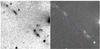 |
Fig. 5 The 40′′ field around the fastest moving knot, MHO 2235-E. See text and the caption of Fig. 4 for details. |
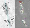 |
Fig. 6 Southern part of MHO 2234. See text and the caption of Fig. 4 for details. The Class 0 protostar MMS3 (aka Ser-emb-1, red circle) is probably the driving source. The yellow circle shows the location of another red YSO from Harvey & Dunham (2009). |
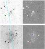 |
Fig. 7 Northern parts of MHO 2234, lower panels show the field included in the NOTCam monitoring field, while the upper panels show the new knot MHO 2234-J further to the north, imaged only once in 2009. The green cross is an artefact. See text and the caption of Fig. 4 for details. |
Proper motion measurements of the 31 brightest knots in the jets.
The multi-epoch proper motion vectors are overlaid in colours on the zoomed images shown in Figs. 4 to 10. Each figure is a zoom-in of a sub-region and shows the H2 line (+continuum) image with knot identification and slit position for K-band spectra in the left panel, and the inverse greyscale with the proper motion vectors overlaid in the right panel. The PM vector length is amplified by a factor 20 for clarity, and every baseline is colour-coded as explained in the caption of Fig. 4.
Multiple PM vectors for the same knot follow more or less the same direction (approximately within the errors of the position angles) from baseline to baseline, for instance knots A1, B, C1 in Fig. 4, knots A2, B1, D1+D2, H1, in Fig. 6, knot I1 in Fig. 7, and knot M4 in Fig. 10. For several knots, however, there is a large directional scatter, such as for knots D, E, and F2 in Figs. 5, and knots G1, H3, H4, H8, in Fig. 6. In these cases the maximum spread of the multi-epoch vectors for one and the same knot can be 90 degrees or more. Most of these are relatively faint or elongated knots, and it could be that we have underestimated the positional uncertainty because of a more difficult centering. Thus, it is unclear whether this scatter is real or if it merely reflects a larger measurement error for these knots.
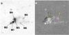 |
Fig. 10 Zoom-in on the HH 476 region (20′′ field), the SW part of MHO 2235 in the NOTCam field. See text and the caption of Fig. 4 for details. The black contours show the Hα emission from 2009 of the previously known Herbig-Haro object HH 476. |
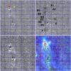 |
Fig. 11 Difference images for part of the MHO 2234 flow including the position of the Class 0 source MMS3 or Ser-emb-1 (red circle) and a not classified YSO from Harvey & Dunham (2009; yellow circle). The image shifts are in the sense: ep2-ep1 (upper left), ep3-ep2 (upper right), and ep4-ep1 (lower left), bright regions showing positive flux. The IRAC/Spitzer 4.5 μm (blue), 5.8 μm (green), and 8 μm (red) is shown with the H2v = 1−0 S(1) line emission in black contours (lower right). |
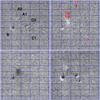 |
Fig. 12 Difference images for part of the MHO 2235 flow including the position of the Class I sources Ser-emb-17 and Ser-emb-11 E and W (red circles) and two YSO candidates from Harvey et al. (2006; magenta circles), cf. Fig. 4. The image shifts are in the direction: ep2-ep1 (upper left), ep3-ep2 (upper right), ep4-ep3 (lower left), and ep4-ep1 (lower right), bright regions showing positive flux. The brightening near knot A1 appeared in the 2011 image and had disappeared again in the 2013 image. |
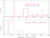 |
Fig. 13 Number distribution of the measured tangential velocities (in km s-1, assuming d = 415 pc). The average velocities over a 10-year timespan from 2003 to 2013 (lower panel) are compared to the more “instantaneous” velocities measured on the shortest timescales of about 2 years (upper panel), the 2011−2013 period (bold red) and the 2009−2011 period (blue). Only knots with proper motion velocities above 2σ (vertical dashed lines) are included. |
In addition to the PM measurements, we made difference images between epochs using the seeing- matched and flux-matched images. Figure 11 shows part of the S arm of the MHO 2234 jet, including knots A1, A2, B1, B2, B3, C, D1, D2, E, and F (cf. Fig. 6), and Fig. 12 shows the same region as that in Fig. 4. When a knot has moved, it shows up as a negative shadow next to a positive peak of emission, although, difference images are also highly sensitive to slight changes in the knot morphology and/or flux. Figure 12 demonstrates the brightening around knot MHO 2235-A1 that appeared some time between 2009 and 2011 and disappeared again some time before the 2013 observations, a clear example of rapid changes in protostellar jets. In general, there is agreement between the PM vectors and the shifts in the difference images.
3.2. Tangential velocities
There has been a discrepancy in the distance estimates to Serpens between the VLBI parallax measurement of EC95 giving a distance of 415 ± 5 pc for the Serpens Main Cluster (Dzib et al. 2010), a neighbouring cloud located <1° to the N, and extinction studies looking at the global properties of the Serpens-Aquila cloud complex, which find smaller distances; 225 ± 55 pc according to Straižys et al. (2003) and 203 ± 7 pc according to Knude (2011). The extinction map of the Serpens-Aquila region shown in Bontemps et al. (2010) and the discussions in Maury et al. (2011) suggest that the N part of the complex, comprising Serpens Main and NH3, is a separate entity from the rest of the complex and located at a larger distance. In this paper we follow this reasoning and adopt 415 pc as the distance. For the longest baseline of about ten years, the uncertainty in the tangential velocity is 12 km s-1, while for the shortest baseline of less than two years, it is 67 km s-1 (see Table 3). The highest velocity measured over the longest baseline is 190 km s-1 for knot MHO 2235-E (see Fig. 5). This scales down to roughly half the value if we apply the 220 ± 80 pc distance estimate (Straižys et al. 2003).
The highest tangential velocities are found for the four knots MHO 2235-E, MHO 2234-A2, MHO 2234-B1, and MHO 2234-D1+D2, but there is an all-over large variation in speed (see Sect. 3.6 for a discussion of time-variable velocities). The median velocities over the longest timescale of ten years are about 50 km s-1, but the scatter is large from 30 to 190 km s-1. These are based on the measurements of only 17 knots, about one-third of all identified knots and about 60% of the knots we were able to measure. Histograms over the velocity distributions are shown in Fig. 13. For the shorter timescales, we are not able to measure the lowest velocities owing to the larger error bar, but it is clear that some knots show high velocities on short timescales, while it averages out on longer timescales. This is evidence of time-variable velocities that shows that knots speed up and slow down.
Six different baselines.
3.3. H2 v = 1–0 S(1) line fluxes
For flux measurements, the images are first seeing-matched using the IRAF task Gauss, which convolves the images with a Gaussian function. All images were matched against the “worst seeing” image using ~50 stars. Secondly, flux matching with respect to ep4 (2013) was performed using the stellar fluxes. The flux-matching error is around 6%; i.e., this is how much the stellar fluxes scatter. We note that many of these stars are young stellar objects (YSOs) currently forming in the region (Djupvik et al. 2006; Harvey et al. 2006, 2007), and YSOs are known to be variable. While a few highly variable stars were discarded before flux matching, low level variability in the stellar sample still might have artificially increased this scatter.
The individual knot fluxes were measured in their apertures using the IRAF task phot. The aperture radii varied from five pixels (1.17′′) for the smallest and faintest to 30 pixels (7′′) for the largest and most diffuse knot, but stayed mostly between five and nine pixels. For elongated knots we used large radii and checked manually that nearby knots did not contaminate the aperture. For each knot the aperture radius was fixed for all epochs, and only its position was redefined. The sky annuli were selected depending on the crowding to minimize contamination.
The flux for the same knot is found to be overall fairly constant in all the four epochs (see Table 4). To search for variability, we calculate the maximum flux variation, i.e. the difference between the lowest and highest flux measured for the same knot. A knot is defined to have flux variability if the maximum flux deviation is larger than three times the standard deviation of the sky background σsky in the deep image of ep4, which is 1.5 × 10⁻¹⁶ erg s-1 cm-2. As shown in Fig. 14, we find flux variability for 13 out of 29 knots. There is no apparent general correlation between flux variability and proper motion.
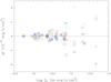 |
Fig. 14 Flux variability detected in 13 of the 29 knots. The deviations from average flux is plotted versus the logarithm of the average flux for each of the knots. Epoch 1 (black circles), epoch 2 (red triangles), epoch 3 (green squares), and epoch 4 (blue stars). Variability is detected whenever the maximum deviation between epochs is greater than 3σ, where σ is the standard deviation of the sky background in the epoch 4 image. The dotted line shows 3σ from average. |
H2v = 1−0 S(1) fluxes of the knots for each of the four epochs.
3.4. Radial velocities
Since the H2 emission is spatially resolved and the emission lines have narrow, essentially Gaussian line profiles, we can use profile fitting to obtain a radial velocity resolution that is much higher than the intrinsic resolution of the observations of 140 km s-1. For each knot we measure the radial velocities from the available H2 lines using the IRAF tasks rvidlines and rvcorrect to obtain the local-standard-of-rest radial velocities (vLSR). The accuracy in the wavelength calibration of our spectra is 0.3 Å or 4 km s-1 (see Sect. 2.3), and since the calibration is done on sky lines in the same spectrum, we do not expect any shifts. The reference wavelengths for the H2 lines are taken from the vacuum wavenumbers provided by Black & van Dishoeck (1987). The number of available lines vary from one to six, depending on the brightness of the knots.
The measured radial velocities are very similar for all lines in the same knot. The adopted error listed in Table 5 is taken to be the rms scatter in the radial velocity measurements line by line rather than the mean error. The Serpens NH3 NE cloud core itself has a mean radial velocity vLSR = 8.5 km s-1 according to Tobin et al. (2011), whose measurement is centred on the Class 0 source MMS3. According to Levshakov et al. (2013), who refer to this cloud core as Do279P6, it is 7.986 km s-1. We apply 8 km s-1 when correcting for the systemic velocity. We assume that the protostar that gives rise to the jet follows the cloud motion so correct for it to find the knot’s radial velocity with respect to the driving source. The radial velocities given in Table 7, with their uncertainties and the number of lines used in the measurement, are thus the LSR velocities corrected for the systemic velocity of the cloud.
The negative radial velocities in the southern MHO 2234 jet and the positive radial velocity for one measurable knot in the northern jet, gives the orientation of the jet along the line of sight. The small number of detected northern knots is likely due to the northern jet moving away from us and into the cloud. The only northern knot that has measurable radial velocity is MHO 2234-J, a bow-shock-shaped feature outside our H2 imaging field, for which we have no proper motion measurements. The knot MHO 2234-A1, for which we have no proper motion because it was too faint in all epochs except for epoch 4, was bright by the time the spectrum was taken and was included in the slit, thus its vrad was obtained together with the one of knot A2. These two knots have the highest measured radial velocity. The radial velocity of MHO 2235-B is very low, but positive, thus the spatial velocity of this knot is towards the SE and away from us.
Radial velocities vrad obtained from the available emission lines, corrected for the systemic velocity of the cloud core of vLSR = 8 km s-1, and the number of lines used to measure vrad.
3.5. Identification of flows and their driving sources
Combining the tangential velocities derived from the proper motions with the radial velocities, available for a subset of the knots, we obtain the space velocities. We use the space velocities, the morphology, and the locations of known protostars listed in Table 6 to evaluate the best candidate driving source for each jet and also to distinguish between separate jet flows and determine which knots belong to which flow. We find at least three separate jet flows, partly overlapping, in the field of view studied.
It should be noted that there are several emission line features that cannot be easily attributed to any of these flows, because they have no velocity information and/or because their location and morphology are difficult to interpret. This concerns in particular the features named Q, R, S, and T in Fig. 2.
Driving source candidates.
3.5.1. Flow 1 and MMS3 (Ser-emb-1)
What we call Flow 1 essentially coincides with the MHO 2234 flow as depicted in Fig. 2. In Djupvik et al. (2006), we suggested that the driving source is the Class 0 source MMS3, also called Ser-emb-1 by Enoch et al. (2009, 2011), who found it to be a single compact source and an early Class 0, probably the least evolved of all protostars in Serpens. The present study confirms that the jet has a bipolar structure with a southern flow (Fig. 6) coming towards us and a northern (Fig. 7) going away from us. From the spatial velocities of the two knots A2 and H1 in the southern arm we estimate an inclination angle of 10−15 degrees with respect to the plane of the sky. This agrees with the VLA velocity maps of Tobin et al. (2011), although their axis of the outflow in the plane of the sky is directly N-S, while both the morphology of the jet, as seen in near- and mid-IR images, as well as the proper motions of the H2 knots, indicate a sky position angle of about ten degrees.
In the S arm we find a spectacular morphology of at least three main structures, each of which consists of curvy whisps of knots that look like fragmented bow shocks, headed by the B knots at ~9′′ from the driving source, the F knots at ~35′′ and the H knots at ~60′′. We speculate that these multiple bow shocks are the result of several bursts of outflow along the jet axis in the recent past, produced by a time-variable jet-ejection mechanism. We do not see a strong bi-polar symmetry though, probably because the northern arm moves slightly into or behind the cloud and is detected at two microns only in two locations: 1) a bubbly and faint multi-knot feature around the I1-2 knots, at (~37′′) from the exciting source; and 2) the clear bow-shock-shaped feature named J, which is at ~120′′ from the driving source. In the 4.5 μm IRAC image, however, there is also extended emission just to the N of the exciting source, most likely the northern component of the bipolar flow moving into the cloud. It is very reddened and not detected at two microns (cf. Fig. 11).
From the velocity information, we find it likely that the southernmost part of the MHO 2234 jet, containing the H1-H8 knots, is indeed part of the N-S going Flow 1 (MHO 2234) and not part of the MHO 2233 structure. Knot H8 apparently moves in the reverse direction, though.
The space velocity of the knots decreases with distance from the originating source, the faster knot being MHO 2234-A2 at a space velocity of 125 km s-1. Its close neighbour A1 is very faint in ep1, and becomes gradually brighter to allow its position to be measured only in epoch 4, but both A1 and A2 are included in the flux measurement aperture and in the slit spectroscopy. As shown in Sect. 9 where we calculate the dynamical ages, the jet from the least evolved protostar shows higher knot velocities than the jet from the more evolved protostars. This is in line with Bontemps et al. (1996), who found roughly an order-of-magnitude higher mechanical-to-bolometric luminosity ratio for outflows from Class 0s compared to Class Is.
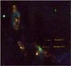 |
Fig. 15 Central part (FOV ≈ 90′′) of the jets colour-coded H2 line filter (red), K-band filter (green), and H-band (blue). N up, E left. |
3.5.2. Flow 2 and Ser-emb-11 binary, E and W
What we call Flow 2 is the longest structure in our 4′ field of view, a NE-SW oriented flow composed of parts of both MHO 2233 (clearly N and P, and probably O) and MHO 2235 (clearly C1, D, E, F, and probably C2, I1, I2, I3). The previously known HH object HH 476, which practically coincides with our group of M knots, is located at an extension of this line, but the proper motion of knot MHO 2235-M4 has a consistent reverse movement, and it is unclear if this group of knots belongs to Flow 2. We also note that the knots MHO 2235-G, H,J, and K could be related to Ser-emb-34, in which case it would be a strongly deflected flow, with no detectable counterjet, but this speculation awaits proper motion measurements. As seen in Fig. 1 and also as noted in the MHO Catalogue (Davis et al. 2010), MHO 2235 may be extending further towards the SW far outside the NOTCam field. Whether this is an extension of Flow 2 or an independent flow is not clear, since we have no velocity information, but no known protostars are found close to these features. The morphology suggests a possible connection, but if both structures to the SW are part of the same flow, this indicates a strong deflection of the jet axis. Thus, Flow 2 could be a parsec-scale flow, with parts of it completely void of emitting knots indicating periods of quiescence in the jet ejection.
Considering the field we have monitored, the knots flowing towards the SW have very clear proper motions and include MHO 2235-E moving at 190 km s-1, the fastest knot in this study. The flow towards NE is more difficult to measure, and only MHO 2233-N has a clear proper motion towards the NE. From the morphology and tangential velocities, we suggest that this flow originates in Ser-emb-11 or in either of the two components of this 2.14′′ separation Class I binary.
After inspecting our supplementary deep JHKS imaging taken simultaneously with H2 line imaging and a narrow-band K continuum filter, we found evidence that our knot MHO 2235-A2, which almost coincides with the protostar Ser-emb-11E, indeed has emission both in the red continuum filter and in the H2 line filter. This source is the easternmost and the fainter of the two Class Is that form the 890 au separation protostar binary Ser-emb-11, which is found by Enoch et al. (2011) to have very extended envelopes and compact disk components. In our images MHO 2235-A2 has a roundish shape, but its psf in the best quality images, where stars have a FWHM of 0.5−0.6′′, is substantially broader. The positions disagree by 0.4′′. The binary companion Ser-emb-11W, which is the brighter of the two in submm wavelengths, is not detected in any near-IR filter. We find no measurable proper motion from MHO 2235-A2. On the other hand, we detect a gradual brightening in flux over the ten years of monitoring in the H2 line filter (see Tables 2 and 4). Thus, what we refer to as knot MHO 2235-A2 may be a mix of continuum emission from the YSO itself (Ser-emb-11E) and some extended line emission.
As shown in Fig. 15 there is a cone of faint emission extending southwards from Ser-emb-11E (at about 5 o’clock) in the K continuum filter and in the H-band. This emission is barely noticeable in the J-band, probably because of high extinction. Such cones of scattered light are usually interpreted as cavities in the envelope carved out by a precessing jet. The part of Flow 2 that we have monitored is a long chain of knots with a slightly S-shaped morphology. This point symmetry is usually interpreted as due to a precessing jet axis. As shown by Fendt & Zinnecker (1998), this is most likely caused by orbital motion of the jet source in a binary (or multiple) system.
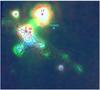 |
Fig. 16 Central ≈45′′ zoom-in of IRAC/Spitzer image shown in Fig. 1. Protostars are marked and labelled. The black contours refer to the 2.1218 μm H2 line emission. |
Measured H2 line fluxes and line ratios.
3.5.3. Flow 3 and Ser-emb-17
Proper motion and radial velocity data show that MHO 2235-B, the brightest of all knots in the images, is moving towards the SE and slightly away from us. From the radial velocity component we determine the inclination angle with respect to the plane of the sky to be 11°. Knot MHO 2235-A1 has a similar proper motion vector, within the errors. These two knots seem to form a separate flow approximately orthogonal to Flow 2 described above. The Class I binary Ser-emb-11 is situated approximately where the two flows cross each other in the plane of the sky. Thus, it is likely that the Flow 3 going SE is either driven by one of the components of the Class I binary Ser-emb-11 or by Ser-emb-17, the proper motion vectors being consistent with both. The Class I source Ser-emb-17 (Enoch et al. 2009, 2011) is located only 12′′ to the NW of the binary Ser-emb-11 and is detected as a faint point source only in the K-continuum and the Ks broad band filters (see Fig. 15). Careful inspection of the IRAC image in Fig. 16 reveals a bridge of H2 emission (green colour gives an emphasis to the 4.5 micron band) between Ser-emb-17 and Ser-emb-11, suggesting a flow in the direction towards MHO 2235-B. The non-detection of this extended emission at two microns is probably due to very high extinction. Ser-emb-17 is located in the densest core in the region according to the N2H+ map of Tobin et al. (2011). Extinction may also explain why we detect no bipolar lobe towards the NW. Based on this and the morphology and velocity of MHO 2235-B, we propose that Ser-emb-17 is the driving source of the jet flowing SE.
Based on jet lengths alone, one would wrongly interpret Flow 3 as the youngest jet in the region. When including the velocity information, however, we find that the furthest away knots in the longer Flow 1 from the Class 0 source have approximately the same dynamical ages (see Sect. 9). A recent study by Giannini et al. (2013) finds a clear correlation of jet length with stellar age, but there were no Class 0 YSOs in their sample of driving sources.
3.6. Time variable velocities
It is evident from the multi-epoch proper motion results presented in Table 2 that the proper motions are not constant over time. Translated to tangential velocities using 415 pc for the distance, the most typical velocity, averaged over ten years, is around 50 km s-1, and the highest velocity is 190 km s-1 as shown in Fig. 13, but short-term proper motions over around two years reveal transient velocities of up to 300 km s-1, such as MHO 2234-B1 from 2009 to 2011 and MHO 2235-E from 2011 to 2013. These are knots that have sped up but move in the same direction as for the other periods. Thus, the H2 knots accelerate and decelerate.
The observable knots are shocks, probably produced by supersonic velocity jumps, for which a natural origin is believed to be a time variable jet ejection speed. Reipurth (1989) suggested that observed knotty jet structures can be explained by episodically pulsed jets, again driven by non-steady accretion in the form of bursts. This was modeled by Raga et al. (1990), and strong evidence for this mechanism was found in the highly symmetric knots in the HH 212 bipolar jet by Zinnecker et al. (1998). The morphology and the knot spacings indirectly point towards time-variable velocities. Direct measurements of time-variability in jet velocities, however, are scarce. This has been detected from multi-epoch studies of a Class II jet in HH 30 (Hartigan & Morse 2007), a Class I binary jet in the L1551 (Bonito et al. 2008), and Class II and Class I jets in the Chamaeleon II star formation region (Caratti o Garatti et al. 2009). It is suggested that Class 0 jets have similar variability behaviour, based on observed knot spacings, but to our knowledge, the present study in Serpens is the first that finds time-variable velocities in a Class 0 jet.
Ejecta at different velocities propagating in a strongly inhomogeneous medium give rise to rather complex interactions and possibly deflections. The jets in Serpens NH3 (Serpens Cluster B) are partly overlapping, and it is not simple to interpret which knot belongs to which flow, considering reverse motion and deflections.
It is believed that faster ejecta may overtake slower ones and potentially change their velocity vectors. Models of randomly pulsed jets by Bonito et al. (2010) predict distinct individual knot velocities, single fast-moving knots, reverse shocks, as well as oblique shocks, the last being produced by reflection at the cocoon surrounding the jet. Our velocity data for the knots in these jets suggest that there are several of these features. The distinct individual knot velocities are clearly demonstrated by our proper motion results. An example of a single fast-moving knot is MHO 2235-E. Possible examples of reversing knots are MHO 2235-M4 and MHO 2234-H8.
Whether a variable jet ejection mechanism is needed to produce the observed time variability in the knot velocities is not enirely clear, and Yirak et al. (2009, 2012) suggest that shocks can be produced by clumps in the jet that collide and merge. If the shocks are due to merging or interacting knots, one would expect variability in the fluxes, as well. The fast-moving elongated knot MHO 2235-E experiences both velocity and flux variability, but in general we find no clear correlation between flux variability and velocity variability or between flux variability and speed.
4. Physical conditions
The knots for which we have K-band spectra are listed with their line fluxes or flux ratios in Table 7. The slit positions are shown overlaid on images in Figs. 4, 6, 7, and 8. All the knots have pure emission line spectra with narrow line profiles, the Gaussian widths being close to the instrument profile, around 10 Å or 140 km s-1. Up to six or seven H2 lines are typically detected in the spectra. There are no other lines or continuum emission. Figure 17 shows knot MHO 2235-B as an example. For all knots the brightest line is the v = 1−0 S(1) line at 2.1218 μm, which contributes on average 59 ± 17% of the total emission in the K band.
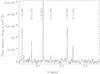 |
Fig. 17 NOTCam K-band (R = 2100) spectrum (slightly smoothed) of the brightest knot MHO 2235-B with the H2 lines marked. Flux density in units of erg s-1 cm-2 Å-1. |
4.1. Extinction
There is substantial cloud extinction in the Serpens NH3 core where these jets are located, and the region is practically opaque in the optical. Even in the K band there is a pronounced decrease in the number of background stars over the region where the jets are located. A lower estimate of AV ~ 20 mag was deduced from the J − H/H − K colour diagram of stars in the surrounding region (Djupvik et al. 2006), which agrees with the extinction map of Bontemps et al. (2010), but these methods “saturate” for the densest regions. There is no emission from the knots in the J and H bands. Deep H-band imaging shows some faint extended emission between some the knots, which we interpret as due to scattered light.
Assuming thermalized gas at a single temperature, we can use the pair of lines originating in the same upper level that are most separated in wavelength, λλ 2.0338 and 2.2233 μm, in order to determine the colour excess between these two wavelengths. We then apply the extinction law Aλ ∝ λ-1.7 to deduce the extinction in terms of visual magnitudes. We have in this manner estimated the extinction to the knots (Table 7) to be in the range 7 <AV< 58 mag. These values are obtained over a narrow wavelength range, however, and their uncertainty may be large. The highest estimate (AV = 58 mag) was found for the knot closest to the Class 0 exciting source. Such high values are rarely found in the literature and, above all, difficult to measure. Davis et al. (2011) compared various techniques to measure the extinction towards molecular hydrogen emission line regions around protostars using integral field spectroscopy and found values reaching up to AV ~ 80 mag close to the protostellar jet sources. In another study of knots from protostellar jets by Caratti o Garatti et al. (2015), an extinction of AV = 50 mag is reported for one of the knots. Knot emission seen through 50 visual magnitudes of extinction (~5 mag at two microns) is weakened by a factor of 100 and must be intrinsically bright.
With this high extinction, one could expect that some knots would be extinguished at 2.1 μm microns, but become observable at 4.5 μm where the extinction is lower; for instance, Flaherty et al. (2007) find that A[ 4.5 ] = 0.53AK. When comparing the areas covered by H2 line imaging with the IRAC images, we conclude that practically all knots found in the mid-IR images are also visible in the near-IR 2.122 μm images, except for two important cases where we believe the extinction is very high: 1) just to the N of the Class 0 exciting source and 2) between MHO2235-B, and its presumably driving source Ser-emb-17. Otherwise, the practically one-to-one correspondence between IRAC and ground-based 2.122 μm images is also in line with what Giannini et al. (2013) finds for the Vela-D molecular cloud, and this suggests that even for relatively high extinction regions, such as in Serpens NH3, near-IR H2 line mapping is able to pick up most of these emission line objects.
4.2. Excitation mechanism
The excitation mechanism of H2 in molecular jets from young stars is mainly due to collisions with other H2 molecules or with H atoms, where typically the lower vibrational levels of the molecule in its ground state get populated. If UV photons are present, however, the higher vibrational levels can also be populated through radiation pumping of H2 into a higher electronic state, followed by a subsequent decay that populates all the vibrational levels of the ground state. A frequently used rule of thumb is that when the ratio v = 2−1 S(1)/v = 1−0 S(1) (2.1477/2.1218) is ≲1/10 and there is an absence of v ≥ 3 lines, the excitation mechanism of H2 is from collisions in a hot gas (Wolfire & Konigl 1991), i.e. due to shocks.
To estimate the excitation temperature and the column densities of H2 in the knots, we construct the Boltzmann diagrams as described in Nisini (2008), where we depart from the Boltzmann distribution that describes a gas in thermal equilibrium 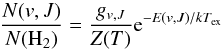 (1)to obtain the result that the natural logarithm of N(v,J) /gv,J, where gv,J are the statistical weights from the selection rules of the transitions, equals −E(v,J) /kTex. Thus, when plotting ln(N(v,J) /gv,J) versus E(v,J), a thermalized gas will give a linear relation, where the slope is the inverse of the excitation temperature Tex. Here, Z(T) is the partition function, and the ro-vibrational energies E(v,J) are taken from Dabrowski (1984). To calculate the relative column densities N(v,J) for a given vibrational and rotational level (v,J), we use the relation N(v,J) = 4πI(v,J) / (hνg(v,J)A(v,J)), where I(v,J) are the measured line intensities obtained from the line fluxes given in Table 7, corrected for extinction using the derived extinction for each knot, and given in units of erg s-1 cm-2 sr-1 using that the spectra cover an area of 0.6″ × 1.9″ across each source. The Einstein coefficients Av,J are from Turner et al. (1977). We fitted a line through the points for each knot, as shown in Fig. 18, and the resulting Tex values and errors are listed in Table 7. Since both the v = 1 and v = 2 vibration levels can be fitted with the same slope, this suggests that the gas is in LTE, and the excitation mechanism is through collisions. The average excitation temperature Tex is 2200 ± 350 K, which is within the typical range of gas temperatures in post-shock regions of protostellar jets (2000−4000 K).
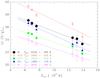 |
Fig. 18 Excitation diagram for the knots listed in Table 7. The entries for each knot are indicated with different symbols and colours and are calculated from the de-reddened line intensities in units of erg s-1 cm-2 sr-1 according to the relation given in the text. Linear fits are made to the points for each knot. Column densities N(v,J) are in the units of cm-2. |
4.3. Ortho-to-para ratio
When H2 molecules are formed, their nuclear spins can either be aligned (ortho) or opposed (para). The ortho-to-para ratio of H2, which refers to these two possible spin states, has been estimated for the vibrationally excited state v = 1 using the line ratios v = 1−0 S(1)/v = 1−0 S(0) and v = 1−0 S(1)/v = 1−0 S(2) following the method of Smith et al. (1997). For each knot we applied the individual extinction estimates as found above, though extinction has a marginal effect on the results. Our values for the ortho-to-para ratios are listed in Table 7 and vary from 2.9 to 4.1 with an average value of 3.3, which is consistent with the expected ratio of 3:1 based on the statistical weights. This very ratio is found in many regions of Herbig-Haro flows. The interpretation could be either 1) that the molecules formed on grains at high temperature according to the statistical weights, and there has been no conversion since; or 2) that collisions with H atoms in the shocked gas has thermalized the level populations and produced this ratio. According to Smith et al. (1997), the latter is the more likely explanation.
4.4. H2 column densities
For the five knots that have spectra taken, we derive the column densities of H2 from the already constructed Boltzmann diagram in Fig. 18. We obtained the values of ln(NH2/Z(T)) by reading off the intercept of each slope at zero Ev,J. The partition function of molecular hydrogen was calculated as Z(T) = 0.024Tex/ (1−e− 6000. /Tex) as given in Smith & Mac Low (1997).
For the remaining knots, we have no spectra and are limited to flux measurements obtained from H2 narrowband imaging in the λ = 2.1218 μm line. We follow the method of Davis et al. (2001) consisting in using this line intensity, together with an assumption on the excitation temperature and the extinction for each knot. We use the average of the four flux measurements given in Table 4. The excitation temperature varies from 1800 to 2620 K among the five knots studied with spectra, and we apply the average value of Tex = 2200 K for all other knots. The extinction apparently varies strongly on small spatial scales and will be the main source of uncertainty using this method. We have estimated the extinction for each knot from a rough spatial interpolation relative to positions for which AV is already measured with spectroscopy as described in Sect. 4.1. This is the best we can do with the available data, and we caution that an error of ten magnitudes in the extinction estimate would lead to an uncertainty factor of 2.8 in the dereddened line intensities and subsequently in the column densities and the luminosities.
The surface area for each knot was estimated individually owing to their different morphologies, and for this we use the deep image from epoch 4. After having subtracted a smoothed version using a 13 × 13 pixel median of the image, for each knot we count those pixels that have fluxes above 3.4 × 10⁻¹⁶ erg s-1 cm-2 arcsec-2, which is 2.3 times the standard deviation of the background. The resulting surface areas for the 29 knots are in the range 1.3 to 10.9 square arc seconds, translating to the range from 5 × 1031 to 4 × 1032 cm2 at 415 pc distance with a median value at 1.3 × 1032 cm2.
We now have dereddened intensities per steradian in the v = 1−0 S(1) line, which is used to calculate the column densities as described in Davis et al. (2001). These are listed in Table 8 in units of H2 molecules per cm-2. The knots are grouped by flows, the first block containing the Flow 1 knots, the second block the Flow 2 knots, and the third block the Flow 3 knots. For the purpose of comparison, we list the results obtained by both methods for those five knots that have spectra, marking the results from spectra with an asterisk. The NH2 obtained from imaging compare reasonably well to the more accurate estimates from spectroscopy, and the column densities are typically within a factor of 2−3, except for knot MHO 2234-A1+A2 where they differ by a factor of five. Thus, the results for knots where we have no spectra should be regarded as approximate and accurate only to within an order of magnitude. The H2 column densities listed in Table 8 compare well with the range of values found in similar studies of knots in protostellar flows. Caratti o Garatti et al. (2015) found H2 column densities from 1017 to 2 × 1020 cm-2 for a sample of 65 knots in flows around 14 sources.
Molecular hydrogen column densities as measured using K-band spectra (5 knots) and narrow-band H2 line imaging (29 knots).
The number densities of molecular hydrogen, nH2, are estimated from the column densities by assuming that the knots’ dimension in the radial direction is equal to their narrowest side seen in the images and measured to be 1.4″ on average. The knots typically have an elongated shape, mainly along the flow direction, which is roughly the orientation of the slits, as well. As learned from the relatively low radial velocities, these jets are flowing practically in the plane of the sky. Thus, applying 1.4″ translates to a jet diameter of 580 au. The derived densities nH2 for each knot are in the range 30−17 000 cm-3 with a median value around 400 cm-3. These densities are very low and indicate either that a low percentage of the jet is molecular or that the jets are lighter than the ambient medium.
4.5. Dynamical ages
On the assumption that velocities are constant, one can calculate the time it has taken for (a part of) a jet to move to its current displacement from the originating source by dividing jet length by velocity. This represents a dynamical age for the observed feature. When velocities slow down with time, the ages are upper limits. We take the jet lengths to be the straight line projections from knot to driving source, corrected for line-of-sight inclinations, but not for any possible deflections. We use the average tangential velocities over ten years coupled with the radial velocities (whenever measurements exist) to get an approximation of the current space velocities of the various parts of the jets. Where we have no radial velocity information, we use the projected length. Table 9 lists our dynamical age estimates for a few features in each of the three flows and demonstrates how recent the jet activity in this region is.
4.6. Mass loss rates
From the column densities, NH2, we can estimate the mass of the H2 gas involved in the emission through the relation  (2)where μ is the mean atomic weight, mH the proton weight, and aknot the area of the emitting region (Nisini et al. 2005). The slit width is substantially narrower than the FWHM of the intensity profiles across the knots. We assume that the knots emit uniformly over their entire surface and use the surface areas derived for each knot as described in the previous section. Thus, we arrive at H2 gas masses in the range from 2 × 10⁻⁸ to 7 × 10⁻⁵M⊙ for the knots (see Table 8). The total mass of H2 gas in each flow is obtained by summing up all the measured knots, and they are listed in Table 10. These estimates are a lower limit to the total H2 gas mass. There are a number of weaker knots for which we do not have reliable flux measurements. It is clear, however, that there is an order of magnitude more mass in the H2 knots of the Class 0 jet (Flow 1) compared to the two Class I jets.
To estimate the H2 mass-loss rates we use the dynamical age, tdyn, derived from the spatial velocities and the separation of each knot to its putative driving source in Table 9 and find Ṁout(H2) = MH2/tdyn per knot. For the 24 knots where we have no radial velocity, we used the average tangential velocities, which for all jets are the dominating vectors of the space velocities, since these all flow practically in the plane of the sky. In this way we obtain the mass flux carried by each knot. As shown in Table 8 the derived mass loss rates per knot are in the range 4 × 10-12M⊙ yr-1<Ṁout(H2) < 10-6M⊙ yr-1. Except for the lowest rates, these values compare well with the mass flow rates estimated for knots in HH 52, HH 53, and HH 54 (Caratti o Garatti et al. 2009). They also compare well to the mass loss rates of 6 × 10⁻¹⁰ to 2 × 10⁻⁶M⊙ yr-1 obtained for nine embedded Class I outflow sources by Davis et al. (2001), although these values are derived in the vicinity of the driving sources. Likewise, Caratti o Garatti et al. (2012) find an average Ṁout(H2) of 3.4 × 10⁻⁹M⊙ yr-1 for five Class Is and six very young YSOs. We have summed up individual knot values to arrive at total values for each flow in Table 10.
Dynamical ages of the knots based on their jet lengths, i.e. separation from the candidate driving source, and their current velocities, v, where we adopt the space velocities when available, and otherwise the tangential velocities on the longest timescale available.
Estimates of total H2 luminosity, mass, mass flow rate, and momentum flux in each flow, as obtained by summing over the individual knots.
The derived mass loss rate is two to three orders of magnitude larger for the Class 0 jet (Flow 1) than for the two Class I jets. This is a combination of the higher mass in the ejecta and the higher knot velocities measured for the Class 0 jet. The momentum flux Ṗ = Ṁvspace for the Class 0 jet (Flow 1) is 1.3 × 10⁻⁴M⊙ km s-1 yr-1, which is almost three orders of magnitude more than the momentum flux in the Class I jets. We note that the three driving sources have a similar bolometric luminosity Lbol ~ 4 L⊙ (Enoch et al. 2011). Thus, among three YSOs with a similar Lbol, the Class 0 jet has significantly higher Ṁout(H2) and Ṗout(H2), suggesting that the difference is due to the earlier evolutionary stage. This is in line with the results of Bontemps et al. (1996), who found a stronger CO outflow momentum from Class 0s than from Class Is and attributed it to a decrease in the mass accretion rate with increasing age of the star. Studies of a larger sample of 23 Class 0 and Class Is by Caratti o Garatti et al. (2006), on the other hand, found no clear distinction between the two YSO classes when examining outflow H2 luminosity versus Lbol. For comparison, we estimate the outflow H2 luminosity from the dereddened flux in the 2.12 μm line, and get L2.12 values of 0.025, 0.0016, and 0.0034 L⊙ for Flow 1, Flow 2, and Flow 3, respectively. The correction factor to apply to L2.12 in order to get LH2 is ~12 when assuming LTE and an average temperature of 2200 K (Caratti o Garatti et al. 2006) and give the values listed in Table 10.
As discussed in Sect. 3.6, our multi-epoch proper motions show that the velocities are time-variable. Thus, all discussions of mass flux here is based on the use of an average velocity over a ten-year time-span for each knot. Within the Class 0 flow, there is a large variation in the estimated mass flow rates of the individual knots. Above all others, MHO 2234-A1+A2, which is the knot nearest to the Class 0 driving source (at a projected distance of ~1800 au), stands out as particularly massive and fast-moving. This double knot alone carries a mass flux of almost 1 × 10⁻⁶M⊙ yr-1 and is the main contributor to the relatively high Ṁout in this flow. It is probably the result of a recent burst of mass accretion, because these mechanisms are believed to be closely coupled.
Still, according to observed relations between the bolometric luminosity of Class 0/Class I sources and their mass flow rate from CO measurements (Shepherd & Churchwell 1996), the expected Ṁout for a 4 L⊙ Class 0 source should be around 10-5M⊙ yr-1. This discrepancy is probably explained by our estimates dealing with only that part of the gas that is involved in the H2 line emission, which is the warm molecular gas component. From these H2 data alone, we have no information about the presence and contribution to the mass-flow rate of a colder molecular gas component or an atomic gas component. Although our deep imaging finds no emission from the knots in the H band where strong [FeII] lines are located, this could be due to high extinction. As shown by Nisini et al. (2005) and Davis et al. (2011), Ṁout of the molecular gas component can be 10 to 1000 times lower than Ṁout from the atomic component.
The ratio of mass outflow to mass accretion, Ṁout/Ṁacc, is typically found to be of the order of 1/10 for Classical T Tauri stars, while there is a large scatter in the measured ratios for younger YSOs from 0.01 to 0.9 depending on tracers used (Antoniucci et al. 2008), while Caratti o Garatti et al. (2012) find an average ratio of 0.01 for Class I and very young YSOs when using Ṁout(H2). If we can assume that the same holds here, we are witnessing a burst of mass accretion about 70 years ago with a mass accretion rate Ṁacc ~ 10-4M⊙ yr-1.
If the velocities were constant, the Ṁout found for a knot would provide a measure of the instantaneous mass flow rate at a given time in the past, and hence give an idea about the accretion history. Although we know from the multi-epoch proper motions that the velocities of many H2 emitting knots may vary with time, we take as a first approximation the average velocities (over 10 years) at face value, as also done when discussing dynamical age. We note the tendency for the space velocities to decrease with distance from the driving source, in particular for the southern arm of the Class 0 jet (Flow 1). Whether this is due to a slowing down of the jets, which could be expected as these shocks travel in a dense medium and may interact with the surrounding gas (entrainment), or it reflects a real variation in ejection speed remains unclear. Also, as mentioned above, it is not clear what percentage of the total mass flux is traced by the shocked molecular hydrogen.
The three protostellar flows studied here are located in the same star forming core, so at the same distance from us, presumably in very similar physical conditions, and in addition, the three driving sources are of similar bolometric luminosities. The knots in the Class 0 jet are both faster and more massive than the knots in the two Class I jets, suggesting a clear difference between the two evolutionary stages and supporting the idea that accretion and ejection is stronger during the Class 0 stage, as suggested by Bontemps et al. (1996). Nevertheless, in view of the emerging picture of the episodic nature of the accretion/ejection phenomenon, which is also supported by our time-variable velocities, we cannot exclude that the observed difference between the Class 0 and the two Class Is presented here is also time-variable. Thus, it could be that we by chance study these sources at a moment dominated by the effects of a recent massive accretion burst in the Class 0 source.
5. Summary and conclusions
We measured proper motions for 31 (out of 57 detected) knots in protostellar jets in the Serpens NH3 region (aka Serpens cluster B), using multi-epoch near-IR H2 line imaging (2.122 μm) with the same telescope/instrument setup over the period 2003 to 2013. Tangential velocities on the timescales: ten years, eight years, six years, four years, and two years were obtained for most of these knots. Radial velocities were obtained for the knots for which we have K-band spectra, using all the available and sufficiently strong H2 lines (typically 4−5 lines), thereby yielding the space velocities. Column densities of H2 were obtained from the dereddened line intensities. For 24 knots without spectra, we estimated column densities through the v = 1−0 S(1) line intensity. The dynamical ages of different parts of these flows were estimated, based on their separations from the driving source and their current velocities, and finally the mass loss rates in the knots were derived. Our results and conclusions are as follows:
-
1.
Based on the knot velocities, the morphology, and published data on protostars in the region, we interpreted our data to show at least three different jet flows in the field we monitored, where two are bipolar. The three driving sources are suggested to be MMS3 (Ser-emb-1), a low luminosity Class 0 source, Ser-emb-11, a binary Class I, and Ser-emb-17, another Class I source, all deeply embedded and previously studied from mid-IR to longer wavelengths.
-
2.
The ten-year baseline proper motions give typical velocities around 50 km s-1 and a maximum velocity of 190 km s-1. While these can be viewed as the average velocities over ten years, the shorter baselines show evidence of time-variable velocities.
-
3.
The knot fluxes over the four measured epochs are relatively stable, and flux variability is detected for 45% of the knots, but only a few vary by as much as 30% or more in their flux. We find no correlation between flux variability and velocity variability, or between flux variability and speed.
-
4.
There was a burst in brightness around MHO 2235-A1 in 2011 as compared to 2009 with a disappearance again in 2013, a clear piece of evidence of the episodic nature of the jets.
-
5.
The deduced dynamical ages are all <5000 yr, and the youngest features <100 yr.
-
6.
Time-variable velocities have been found in the ejecta from a Class 0 source for the first time. We also found that the Class 0 jet has higher measured velocities than the two Class I jets.
-
7.
From the K-band spectra obtained for a subset of the brighter knots, we estimated the excitation temperatures, the average value being Tex = 2200 ± 350 K, which is typical of ro-vibrational states of H2 in post-shock layers. Towards these knots we have also made a rough estimate of the extinction using the H2 lines, and found values as high as AV = 58 mag.
-
8.
We find that Ṁout for the Class 0 jet is about two orders of magnitude higher than Ṁout for the two Class I jets while the Lbol of the driving sources are all practically the same.
Nordic-Baltic Optical/NIR and Radio Astronomy Summer School: “Star Formation in the Milky Way and Nearby Galaxies”, 8−18 June 2009, Turku, Finland. See URL http://www.not.iac.es/tuorla2009/local/
NOTCam is documented in detail on the URL http://www.not.iac.es/instruments/notcam/
IRAF is distributed by the National Optical Astronomy Observatory, which is operated by the Association of Universities for Research in Astronomy (AURA) under cooperative agreement with the National Science Foundation.
Acknowledgments
We thank the anonymous referee for suggestions that led to a substantial improvement of the article. A.A.D. thanks A.J. Delgado and G. Gahm for fruitful discussions. This work was initiated as one of the student projects during the Nordic-Baltic Optical/NIR and Radio Astronomy Summer School held in the Tuorla Observatory, Turku, Finland on 8−18th June 2009, where the financial support from NordForsk is greatly acknowledged. We have made extensive use of SAOImage DS9, developed by Smithsonian Astrophysical Observatory. This work made use of EURO-VO software TOPCAT, which is funded by the European Commission through contracts RI031675 (DCA) and 011892 (VO-TECH) under the 6th Framework Programme and contracts 212104 (AIDA) and 261541 (VO-ICE) under the 7th Framework Programme. T.L. acknowledges the support of the Estonian Ministry for Education and Science, as well as European Social Fund’s Doctoral Studies and Internationalisation Programme DoRa and Kristjan Jaak Scholarship, which are carried out by Foundation Archimedes. This work is partly based on observations made with the Spitzer Space Telescope, which is operated by the Jet Propulsion Laboratory, California Institute of Technology under a contract with NASA.
References
- Antoniucci, S., Nisini, B., Giannini, T., & Lorenzetti, D. 2008, A&A, 479, 503 [NASA ADS] [CrossRef] [EDP Sciences] [Google Scholar]
- Bacciotti, F., Whelan, E. T., Alcalá, J. M., et al. 2011, ApJ, 737, L26 [NASA ADS] [CrossRef] [Google Scholar]
- Black, J. H., & van Dishoeck, E. F. 1987, ApJ, 322, 412 [NASA ADS] [CrossRef] [Google Scholar]
- Bonito, R., Fridlund, C. V. M., Favata, F., et al. 2008, A&A, 484, 389 [NASA ADS] [CrossRef] [EDP Sciences] [Google Scholar]
- Bonito, R., Orlando, S., Peres, G., et al. 2010, A&A, 511, A42 [NASA ADS] [CrossRef] [EDP Sciences] [Google Scholar]
- Bontemps, S., Andre, P., Terebey, S., & Cabrit, S. 1996, A&A, 311, 858 [NASA ADS] [Google Scholar]
- Bontemps, S., André, P., Könyves, V., et al. 2010, A&A, 518, L85 [NASA ADS] [CrossRef] [EDP Sciences] [Google Scholar]
- Brand, J., Cesaroni, R., Caselli, P., et al. 1994, A&AS, 103, 541 [NASA ADS] [Google Scholar]
- Caratti o Garatti, A., Giannini, T., Nisini, B., & Lorenzetti, D. 2006, A&A, 449, 1077 [NASA ADS] [CrossRef] [EDP Sciences] [Google Scholar]
- Caratti o Garatti, A., Eislöffel, J., Froebrich, D., et al. 2009, A&A, 502, 579 [NASA ADS] [CrossRef] [EDP Sciences] [Google Scholar]
- Caratti o Garatti, A., Garcia Lopez, R., Antoniucci, S., et al. 2012, A&A, 538, A64 [NASA ADS] [CrossRef] [EDP Sciences] [Google Scholar]
- Caratti o Garatti, A., Stecklum, B., Linz, H., Garcia Lopez, R., & Sanna, A. 2015, A&A, 573, A82 [NASA ADS] [CrossRef] [EDP Sciences] [Google Scholar]
- Cohen, M., & Kuhi, L. V. 1979, ApJS, 41, 743 [NASA ADS] [CrossRef] [Google Scholar]
- Dabrowski, I. 1984, Can. J. Phys., 62, 1639 [NASA ADS] [CrossRef] [Google Scholar]
- Davis, C. J., Ray, T. P., Desroches, L., & Aspin, C. 2001, MNRAS, 326, 524 [NASA ADS] [CrossRef] [Google Scholar]
- Davis, C. J., Gell, R., Khanzadyan, T., Smith, M. D., & Jenness, T. 2010, A&A, 511, A24 [NASA ADS] [CrossRef] [EDP Sciences] [Google Scholar]
- Davis, C. J., Cervantes, B., Nisini, B., et al. 2011, A&A, 528, A3 [NASA ADS] [CrossRef] [EDP Sciences] [Google Scholar]
- Djupvik, A. A., & Andersen, J. 2010, in Highlights of Spanish Astrophysics V, eds. J. M. Diego, L. J. Goicoechea, J. I. González-Serrano, & J. Gorgas, 211 [Google Scholar]
- Djupvik, A. A., André, P., Bontemps, S., et al. 2006, A&A, 458, 789 [NASA ADS] [CrossRef] [EDP Sciences] [Google Scholar]
- Dzib, S., Loinard, L., Mioduszewski, A. J., et al. 2010, ApJ, 718, 610 [NASA ADS] [CrossRef] [Google Scholar]
- Eiroa, C., Djupvik, A. A., & Casali, M. M. 2008, in Handbook of Star Forming Regions, Vol. II, ed. B. Reipurth, 693 [Google Scholar]
- Enoch, M. L., Evans, II, N. J., Sargent, A. I., & Glenn, J. 2009, ApJ, 692, 973 [NASA ADS] [CrossRef] [Google Scholar]
- Enoch, M. L., Corder, S., Duchêne, G., et al. 2011, ApJS, 195, 21 [NASA ADS] [CrossRef] [Google Scholar]
- Fazio, G. G., Hora, J. L., Allen, L. E., et al. 2004, ApJS, 154, 10 [NASA ADS] [CrossRef] [Google Scholar]
- Fendt, C., & Zinnecker, H. 1998, A&A, 334, 750 [NASA ADS] [Google Scholar]
- Flaherty, K. M., Pipher, J. L., Megeath, S. T., et al. 2007, ApJ, 663, 1069 [CrossRef] [Google Scholar]
- Frank, A., Ray, T. P., Cabrit, S., et al. 2014, in Protostars and Planets VI, eds. H. Beuther, R. S. Klessen, C. P. Dullemond, & T. Henning (Tucson: University of Arizona Press), 451 [Google Scholar]
- Giannini, T., Lorenzetti, D., De Luca, M., et al. 2013, ApJ, 767, 147 [NASA ADS] [CrossRef] [Google Scholar]
- Hartigan, P., & Morse, J. 2007, ApJ, 660, 426 [NASA ADS] [CrossRef] [Google Scholar]
- Harvey, P., & Dunham, M. M. 2009, ApJ, 695, 1495 [NASA ADS] [CrossRef] [Google Scholar]
- Harvey, P. M., Chapman, N., Lai, S.-P., et al. 2006, ApJ, 644, 307 [NASA ADS] [CrossRef] [Google Scholar]
- Harvey, P., Merín, B., Huard, T. L., et al. 2007, ApJ, 663, 1149 [NASA ADS] [CrossRef] [Google Scholar]
- Knude, J. 2011, ArXiv e-prints [arXiv:1103.0455] [Google Scholar]
- Levshakov, S. A., Henkel, C., Reimers, D., et al. 2013, A&A, 553, A58 [NASA ADS] [CrossRef] [EDP Sciences] [Google Scholar]
- Maury, A. J., André, P., Men’shchikov, A., Könyves, V., & Bontemps, S. 2011, A&A, 535, A77 [Google Scholar]
- Nisini, B. 2008, in Jets from Young Stars II, eds. F. Bacciotti, L. Testi, & E. Whelan (Berlin: Springer Verlag), Lect. Notes Phys., 742, 79 [Google Scholar]
- Nisini, B., Bacciotti, F., Giannini, T., et al. 2005, A&A, 441, 159 [NASA ADS] [CrossRef] [EDP Sciences] [Google Scholar]
- Oliva, E., Origlia, L., Maiolino, R., et al. 2013, A&A, 555, A78 [NASA ADS] [CrossRef] [EDP Sciences] [Google Scholar]
- Raga, A. C., Binette, L., Canto, J., & Calvet, N. 1990, ApJ, 364, 601 [NASA ADS] [CrossRef] [Google Scholar]
- Reipurth, B. 1989, Nature, 340, 42 [NASA ADS] [CrossRef] [Google Scholar]
- Reipurth, B., & Bally, J. 2001, ARA&A, 39, 403 [NASA ADS] [CrossRef] [Google Scholar]
- Shepherd, D. S., & Churchwell, E. 1996, ApJ, 472, 225 [NASA ADS] [CrossRef] [Google Scholar]
- Skrutskie, M. F., Cutri, R. M., Stiening, R., et al. 2006, AJ, 131, 1163 [NASA ADS] [CrossRef] [Google Scholar]
- Smith, M. D., & Mac Low, M.-M. 1997, A&A, 326, 801 [NASA ADS] [Google Scholar]
- Smith, M. D., Davis, C. J., & Lioure, A. 1997, A&A, 327, 1206 [NASA ADS] [Google Scholar]
- Straižys, V., Černis, K., & Bartašiūtė, S. 2003, A&A, 405, 585 [NASA ADS] [CrossRef] [EDP Sciences] [Google Scholar]
- Tobin, J. J., Hartmann, L., Chiang, H.-F., et al. 2011, ApJ, 740, 45 [NASA ADS] [CrossRef] [Google Scholar]
- Tokunaga, A. T., & Vacca, W. D. 2005, PASP, 117, 421 [NASA ADS] [CrossRef] [Google Scholar]
- Turner, J., Kirby-Docken, K., & Dalgarno, A. 1977, ApJS, 35, 281 [Google Scholar]
- Wolfire, M. G., & Konigl, A. 1991, ApJ, 383, 205 [NASA ADS] [CrossRef] [Google Scholar]
- Yirak, K., Frank, A., Cunningham, A. J., & Mitran, S. 2009, ApJ, 695, 999 [NASA ADS] [CrossRef] [Google Scholar]
- Yirak, K., Schroeder, E., Frank, A., & Cunningham, A. J. 2012, ApJ, 746, 133 [NASA ADS] [CrossRef] [Google Scholar]
- Ziener, R., & Eislöffel, J. 1999, A&A, 347, 565 [NASA ADS] [Google Scholar]
- Zinnecker, H., McCaughrean, M. J., & Rayner, J. T. 1998, Nature, 394, 862 [NASA ADS] [CrossRef] [PubMed] [Google Scholar]
All Tables
Radial velocities vrad obtained from the available emission lines, corrected for the systemic velocity of the cloud core of vLSR = 8 km s-1, and the number of lines used to measure vrad.
Molecular hydrogen column densities as measured using K-band spectra (5 knots) and narrow-band H2 line imaging (29 knots).
Dynamical ages of the knots based on their jet lengths, i.e. separation from the candidate driving source, and their current velocities, v, where we adopt the space velocities when available, and otherwise the tangential velocities on the longest timescale available.
Estimates of total H2 luminosity, mass, mass flow rate, and momentum flux in each flow, as obtained by summing over the individual knots.
All Figures
|
Fig. 1 Overview of the Serpens/G3-G6 region (also called Serpens Cluster B and the Serpens NH3 cloud) as seen by IRAC/Spitzer in 3.6 μm (blue), 4.5 μm (green), and 8 μm (red). N up, E left. Total FOV ≈ 15′ × 15′. The jets are mainly enhanced in the 4.5 μm band. The ≈4′ field monitored with NOTCam for proper motions is marked white and shown in Fig. 2. The white arrows point to two bow-shock shaped features outside our monitored field to the N and NE and two jet-like features in the SW region. |
| In the text | |
|
Fig. 2 Deep H2 + continuum (2.122 μm) narrowband NOTCam image of the ≈4′ field observed in this multi-epoch study. N up, E left. Naming of jet structures according to the MHO Catalogue is sketched: MHO 2233 (magenta), MHO 2234 (blue), and MHO 2235 (green). The previously known HH 476 is labelled. Red circles show the positions of Class 0 and Class I protostars, the ID number according to designations by Enoch et al. (2009); for instance, 1 refers to the Class 0 source Ser-emb-1, which is named MMS3 in Djupvik et al. (2006). Only a few knots are identified with letters here, and the majority are identified in zoomed-in regions in the following figures. |
| In the text | |
|
Fig. 3 Relative position accuracy between epochs checked on stars after the final registration (panels ΔX and ΔY) and flux matching accuracy checked after seeing and flux matching (lower panels). The ΔX and ΔY values are the offsets in X and Y (in pixels) between the measured epoch and the reference epoch (i.e. epoch 4). Epoch 1 is shown to the left, epoch 2 in the centre, and epoch 3 to the right, all plotted with respect to reference X-pixel. In the lower panels we show the flux ratio for the same stars. Black dots indicate all stars, red crosses show stars rejected due to large FWHM and/or high flux ratio, and blue circles indicate stars used for the accuracy calculations. |
| In the text | |
|
Fig. 4 Central 50′′ field comprising the MHO 2235 NE part. N up, E left. Left: epoch 4 image overlaid with knot identification and slit position for K-band spectroscopy. Right: Ep4 image with proper motion vectors, amplified by a factor 20 for clarity. The color coding of the pm vectors is as follows: PM14 (blue), PM12 (red), PM13 (green), PM24 (cyan), PM23 (yellow), PM34 (magenta). Protostars are shown with red circles. Ser-emb-11 E and W (a binary Class I) and Ser-emb-17 are strong candidate driving sources. Magenta circles denote YSO candidates from Harvey et al. (2006). The maser refers to an H2O maser position from Brand et al. (1994). |
| In the text | |
|
Fig. 5 The 40′′ field around the fastest moving knot, MHO 2235-E. See text and the caption of Fig. 4 for details. |
| In the text | |
|
Fig. 6 Southern part of MHO 2234. See text and the caption of Fig. 4 for details. The Class 0 protostar MMS3 (aka Ser-emb-1, red circle) is probably the driving source. The yellow circle shows the location of another red YSO from Harvey & Dunham (2009). |
| In the text | |
|
Fig. 7 Northern parts of MHO 2234, lower panels show the field included in the NOTCam monitoring field, while the upper panels show the new knot MHO 2234-J further to the north, imaged only once in 2009. The green cross is an artefact. See text and the caption of Fig. 4 for details. |
| In the text | |
 |
Fig. 8 North-eastern part of MHO 2233 (37′′ field). See text and the caption of Fig. 4 for details. |
| In the text | |
 |
Fig. 9 SW part of MHO 2235 (47′′ field). See text and the caption of Fig. 4 for details. |
| In the text | |
|
Fig. 10 Zoom-in on the HH 476 region (20′′ field), the SW part of MHO 2235 in the NOTCam field. See text and the caption of Fig. 4 for details. The black contours show the Hα emission from 2009 of the previously known Herbig-Haro object HH 476. |
| In the text | |
|
Fig. 11 Difference images for part of the MHO 2234 flow including the position of the Class 0 source MMS3 or Ser-emb-1 (red circle) and a not classified YSO from Harvey & Dunham (2009; yellow circle). The image shifts are in the sense: ep2-ep1 (upper left), ep3-ep2 (upper right), and ep4-ep1 (lower left), bright regions showing positive flux. The IRAC/Spitzer 4.5 μm (blue), 5.8 μm (green), and 8 μm (red) is shown with the H2v = 1−0 S(1) line emission in black contours (lower right). |
| In the text | |
|
Fig. 12 Difference images for part of the MHO 2235 flow including the position of the Class I sources Ser-emb-17 and Ser-emb-11 E and W (red circles) and two YSO candidates from Harvey et al. (2006; magenta circles), cf. Fig. 4. The image shifts are in the direction: ep2-ep1 (upper left), ep3-ep2 (upper right), ep4-ep3 (lower left), and ep4-ep1 (lower right), bright regions showing positive flux. The brightening near knot A1 appeared in the 2011 image and had disappeared again in the 2013 image. |
| In the text | |
|
Fig. 13 Number distribution of the measured tangential velocities (in km s-1, assuming d = 415 pc). The average velocities over a 10-year timespan from 2003 to 2013 (lower panel) are compared to the more “instantaneous” velocities measured on the shortest timescales of about 2 years (upper panel), the 2011−2013 period (bold red) and the 2009−2011 period (blue). Only knots with proper motion velocities above 2σ (vertical dashed lines) are included. |
| In the text | |
|
Fig. 14 Flux variability detected in 13 of the 29 knots. The deviations from average flux is plotted versus the logarithm of the average flux for each of the knots. Epoch 1 (black circles), epoch 2 (red triangles), epoch 3 (green squares), and epoch 4 (blue stars). Variability is detected whenever the maximum deviation between epochs is greater than 3σ, where σ is the standard deviation of the sky background in the epoch 4 image. The dotted line shows 3σ from average. |
| In the text | |
|
Fig. 15 Central part (FOV ≈ 90′′) of the jets colour-coded H2 line filter (red), K-band filter (green), and H-band (blue). N up, E left. |
| In the text | |
|
Fig. 16 Central ≈45′′ zoom-in of IRAC/Spitzer image shown in Fig. 1. Protostars are marked and labelled. The black contours refer to the 2.1218 μm H2 line emission. |
| In the text | |
|
Fig. 17 NOTCam K-band (R = 2100) spectrum (slightly smoothed) of the brightest knot MHO 2235-B with the H2 lines marked. Flux density in units of erg s-1 cm-2 Å-1. |
| In the text | |
|
Fig. 18 Excitation diagram for the knots listed in Table 7. The entries for each knot are indicated with different symbols and colours and are calculated from the de-reddened line intensities in units of erg s-1 cm-2 sr-1 according to the relation given in the text. Linear fits are made to the points for each knot. Column densities N(v,J) are in the units of cm-2. |
| In the text | |
Current usage metrics show cumulative count of Article Views (full-text article views including HTML views, PDF and ePub downloads, according to the available data) and Abstracts Views on Vision4Press platform.
Data correspond to usage on the plateform after 2015. The current usage metrics is available 48-96 hours after online publication and is updated daily on week days.
Initial download of the metrics may take a while.