| Issue |
A&A
Volume 586, February 2016
|
|
|---|---|---|
| Article Number | A8 | |
| Number of page(s) | 15 | |
| Section | Extragalactic astronomy | |
| DOI | https://doi.org/10.1051/0004-6361/201526950 | |
| Published online | 19 January 2016 | |
Halo dust detection around NGC 891⋆
1 INAF–Osservatorio Astrofisico di
Arcetri, Largo Enrico Fermi 5 50125 Firenze Italy
e-mail: This email address is being protected from spambots. You need JavaScript enabled to view it.
2 INAF–Osservatorio Astronomico di
Roma, via di Frascati 33, 00040
Monteporzio,
Italy
Received: 13 July 2015
Accepted: 23 September 2015
Abstract
Context. Observations of edge-on galaxies allow us to investigate the vertical extent and properties of dust, gas and stellar distributions. NGC 891 has been studied for decades and represents one of the best studied cases of an edge-on galaxy.
Aims. We use deep Photoconductor Array Camera and Spectrometer (PACS) data together with Infrared Array Camera (IRAC), Multiband Imaging Photometer for Spitzer (MIPS) and Spectral and Photometric Imaging Receiver (SPIRE) data to study the vertical extent of dust emission around NGC 891. We also test for the presence of a more extended, thick dust component.
Methods. By performing a convolution of an intrinsic vertical profile emission with each instrument point spread function (PSF) and comparing it with observations we derived the scale height of a thin and thick dust-disc component.
Results. The emission is best fit with the sum of a thin and a thick dust component for all wavelengths considered. The scale height of both dust components shows a gradient goes from 70 μm to 250 μm. This could be due either to a drop in dust heating (and thus the dust’s temperature) with the distance from the plane, or to a sizable contribution (~15–80%) of an unresolved thin disc of hotter dust to the observed surface brightness at shorter wavelengths. The scale height of the thick dust component, using observations from 70 μm to 250 μm, has been estimated at (1.44 ± 0.12) kpc, which is consistent with previous estimates (i.e. extinction and scattering in optical bands and mid-infrared (MIR) emission). The amount of dust mass at distances greater than ~2 kpc from the midplane represents 2–3.3% of the total galactic dust mass, and the abundance of small grains relative to large grains is almost halved compared to levels in the midplane.
Conclusions. The paucity of small grains high above the midplane might indicate that dust is hit by interstellar shocks or galactic fountains and entrained together with gas. The halo dust component is likely to be embedded in an atomic/molecular gas and heated by a thick stellar disc.
Key words: galaxies: structure / galaxies: individual: NGC 891 / galaxies: spiral / dust, extinction / submillimeter: galaxies / infrared: galaxies
Herschel is an ESA space observatory with science instruments provided by European-led Principal Investigator consortia and with important participation from NASA.
© ESO, 2016
1. Introduction
Nearby edge-on spiral galaxies offer a special opportunity to learn about the vertical structure and properties of dust, gas, and stellar distributions that extend out from the galaxy midplane. Several galaxies of this class have been observed in optical bands and show many common properties. The high inclination of these galaxies makes them particularly well-suited to multi-wavelength studies of the vertical structure of their disc. Fitting optical images with radiative transfer models allows information on the dust and stellar distributions to be obtained. Stars and dust are found to follow an exponential distribution, both radially and vertically: the dust radial scale length is ~1.4 times larger than that of the stellar distribution while its vertical scale height is about half of that of stars (Kylafis & Bahcall 1987; Xilouris et al. 1997, 1998, 1999; Alton et al. 2004; Bianchi 2007; Baes et al. 2010; De Looze et al. 2012; De Geyter et al. 2014).
Extending studies further out to galactic haloes, there is increasing evidence of dusty clouds up to a few kpc from the galactic disc that seem to be related to the disc-halo cycle (e.g. Howk 2012). Direct optical imaging of edge-on galaxies often shows extraplanar filaments of dense clouds backlit by stars (Howk & Savage 1997, 1999, 2000; Rossa et al. 2004; Thompson et al. 2004; Howk 2005). An estimate of the mass of dust contained in these clouds indicate that a relevant percentage of dust can be lifted to these vertical distances without being destroyed (Howk 2005).
Moving even further from the galaxy main body, Zaritsky (1994) observed dust extinction up to 200 kpc out in the galactic haloes of two nearby galaxies, NGC 2835 and NGC 3521. This result was supported by Ménard et al. (2010) who measured the extinction of background quasars that correlate to local galaxies and found evidence for dust in the intergalactic medium (IGM) up to 1 Mpc from galactic centres.
GALEX and Swift observations in UV bands by Hodges-Kluck & Bregman (2014) reveal diffuse UV light around late-type galaxies out to 5–20 kpc from the galactic disc. The emission is rather blue and not consistent with light from extraplanar stars; the favoured hypothesis is that this emission escapes from the galactic disc and scatters off dust in the halo. This finding is consistent with the extinction measurements from Ménard et al. (2010), therefore corroborating the evidence for dust in galactic haloes.
With the advent of Spitzer, and more recently of Herschel (Pilbratt et al. 2010), we have the necessary sensitivity to observe extraplanar dust thermal emission directly. Aromatic bands have been observed as far as 6 kpc above the disc of NGC 5907 (Irwin & Madden 2006) and in galactic winds around several nearby sources (McCormick et al. 2013). Continuum dust emission up to a similar height was found in NGC 891 by Burgdorf et al. (2007).
In this paper we focus on the vertical dust distribution in the well-known edge-on galaxy, NGC 891. This galaxy is 9.6 Mpc (e.g. Strickland et al. 2004) from Earth and it has an inclination of ≃89.7° (Xilouris et al. 1999). The dust distribution follows an exponential profile with a scale length of hd ~ 8 kpc and a scale height of zd ~ 0.3 kpc, thinner than the stellar distribution but more radially extended (Xilouris et al. 1999). Radiative transfer models by Bianchi (2008) and Popescu et al. (2000a, 2011), starting with models by Xilouris et al. (1999), are able to reproduce the dust spectral energy distribution (SED); thus the radiation field across the galaxy is reliably modelled. The galactic stellar distribution comprises the two classical components, an old stellar bulge and an old stellar disc, with the addition of a clumpy component that is confined in a very thin region at the centre of the main disc. Bianchi & Xilouris (2011), using the results from the 3D radiative transfer model from Bianchi (2008) are able to reproduce most of the characteristics of far-infrared (FIR) and sub-mm images obtained with the SPIRE instrument onboard Herschel.
 |
Fig. 1 From top to bottom: IRAC 8 μm (after stellar
subtraction), MIPS 24 μm, PACS 70 μm (left
column) and PACS 100 and 160 μm and SPIRE 250 μm (right
column) images of NGC 891. Each panel shows an area of ~14′ × 7′ centred on the galaxy’s
radio continuum coordinates α = 2h22m33 |


Optical broadband observations obtained by Howk & Savage (1997) with the WIYN 3.5-m telescope revealed a complex dusty structure above the galactic plane up to a distance of z ≲ 2 kpc. Dust emission was later directly detected by Burgdorf et al. (2007) with the Infrared Spectrograph aboard Spitzer at 16 and 22 μm. In particular, the surface brightness at 22 μm drops following an exponential decay with a scaleheight of 1.3 ± 0.3 kpc, which is consistent with the optical measurements by Howk & Savage (1997). Furthermore, Kamphuis et al. (2007), using MIPS 24 μm observations, detect dust emission up to ~2 kpc from the galactic plane and Whaley et al. (2009), using multi-wavelength observations, find extraplanar dust emission and aromatic features up to a vertical distance of z ≳ 2.5 kpc. However, Kamphuis et al. (2007) and Whaley et al. (2009) do not consider the effects of the instruments point spread function (PSF) in detail and, therefore, their measurements are to be considered qualitative.
More recently, Seon & Witt (2012) have reported on the discovery of a UV halo due to the diffuse dust present above the galactic plane of NGC 891 and Seon et al. (2014), using a 3D radiative transfer model, have found that the UV halo is well reproduced by a model with two exponential dust discs, one with a scaleheight of 0.2–0.25 kpc and a wider component with a scaleheight of 1.2–2.0 kpc.
In this work, we use Spitzer and Herschel data (from 8 to 250 μm) to study the extent of dust emission above the galactic plane, taking a particular care in the analysis of the effects of the instruments PSF. We then compare the derived dust distribution to the extinction and emission measurements from the literature. This paper is organised as follows: Sect. 2 presents the observations and the data reduction used to retrieve the data; Sect. 3 shows the dust emission profile as measured by Spitzer and Herschel instruments. In Sect. 4 we highlight the variability of the vertical profile along the major axis of the galaxy; Sect. 5 shows measurements of the dust SED, temperature and optical depth at different vertical distances. In Sect. 6 we discuss our results, and in Sect. 7 we draw our conclusions.
2. Observations and data reduction
Herschel Photoconductor Array Camera and Spectrometer (PACS, Poglitsch et al. 2010) photometric observations were
taken at 70, 100 and 160 μm as part of the Herschel EDGE-on
galaxy Survey (HEDGES; PI: E. Murphy). The 70 and 100 μm data consist of two
cross-scans at a 20′′
s-1 scan speed (Obs
IDs: 1342261790, 1342261792 for 70 μm and Obs IDs: 1342261791, 1342261793 for 100
μm), while
160 μm
observations consist of four cross-scans at 20′′ s-1 scan speed (Obs IDs: 1342261790, 1342261791, 1342261792,
1342261793). The Herschel interactive processing environment (HIPE,
v.12.1.0; Ott 2010) was first used to bring the raw
Level-0 data to Level-1 using the PACS calibration tree PACS_CAL_65_0. Maps were then
produced using Scanamorphos (v.24.0, Roussel 2013).
Images were produced with pixel sizes of  , 2′′, and 3′′, respectively (Fig. 1). We compared these observations with the less deep observations that
were obtained as part of the guaranteed time key project Very Nearby Galaxy Survey (VNGS;
KPGT_cwilso01_1; PI: C. D. Wilson) and find agreement between the two datasets. In addition,
deeper observations are available from the Open Time program, OT1_sveilleu_2 (PI: S.
Veilleux). However, the field of view is too narrow and border effects would be introduced
in the vertical profile; consequently, we therefore decided not to use this dataset.
, 2′′, and 3′′, respectively (Fig. 1). We compared these observations with the less deep observations that
were obtained as part of the guaranteed time key project Very Nearby Galaxy Survey (VNGS;
KPGT_cwilso01_1; PI: C. D. Wilson) and find agreement between the two datasets. In addition,
deeper observations are available from the Open Time program, OT1_sveilleu_2 (PI: S.
Veilleux). However, the field of view is too narrow and border effects would be introduced
in the vertical profile; consequently, we therefore decided not to use this dataset.
Herschel SPIRE (Griffin et al. 2010) photometric observations at 250 μm were obtained as part of the VNGS (Obs ID: 1342189430). The galaxy was observed in large map mode, covering an area of 20′ × 20′ centred on the object with two cross-scans, using a 30 s-1 scan rate. Data were reduced with HIPE using the SPIRE calibration tree SPIRE_CAL_12_3 and the standard pipeline destriper to remove baselines. The map was then produced using the naïve map-making procedure within HIPE. The resulting image has a uniform background and pixel size of 6′′ (Fig. 1). In-beam flux densities are converted to surface brightness, assuming an effective beam solid angle Ω = 465 arcsec2 (SPIRE Handbook, 20141). SPIRE observations at 350 and 500 μm were also obtained as part of the VNGS, but these were not used here since the instrument resolution at these wavelengths is too low for our purposes.
Spitzer IRAC individual Basic Calibrated Data (BCD) frames were taken from
the combined observations (eight Astronomical Observing Requests) acquired by G. Fazio
(Spitzer Cycle 1, PID 3), and processed with version 18.25.0 of the SSC
pipeline. The data were acquired in high dynamic range (HDR) mode, so that each frame
consists of one short integration and two long integrations. The 442 long-integration time
BCDs were combined into a single mosaic with MOPEX (Makovoz
& Marleau 2005). Bad pixels, i.e. pixels masked in the data collection event
(DCE) status files and in the static masks (pmasks), were ignored. Additional inconsistent
pixels were removed by means of the MOPEX outlier rejection algorithms. We relied on both
the box and the dual outlier techniques, together with the multiframe reject algorithm. The
frames were corrected for geometrical distortion and projected on to a north-east coordinate
system with pixel sizes of  , roughly half the size of the original
pixels. The final mosaics were then obtained with standard linear interpolation. The same
was done for the uncertainty images, i.e. the maps for the standard deviations of the data
frames. After experimenting with various HDR correction algorithms, we neglected this
correction as it resulted in inferior final mosaics. Despite several attempts at image
reduction, the IRAC Channel 4 image (see Fig. 1) still
shows a residual column bleed, which is visible towards the southwest part of the image.
However, these artefacts do not affect our analysis as they are masked out when necessary.
To obtain the “dust map” at 8 μm we subtract the stellar component following the
prescription by Helou et al. (2004): we scale the
IRAC 3.6 μm map
by 0.232 and we subtract it from the observed IRAC 8 μm map on a pixel-by-pixel
basis.
, roughly half the size of the original
pixels. The final mosaics were then obtained with standard linear interpolation. The same
was done for the uncertainty images, i.e. the maps for the standard deviations of the data
frames. After experimenting with various HDR correction algorithms, we neglected this
correction as it resulted in inferior final mosaics. Despite several attempts at image
reduction, the IRAC Channel 4 image (see Fig. 1) still
shows a residual column bleed, which is visible towards the southwest part of the image.
However, these artefacts do not affect our analysis as they are masked out when necessary.
To obtain the “dust map” at 8 μm we subtract the stellar component following the
prescription by Helou et al. (2004): we scale the
IRAC 3.6 μm map
by 0.232 and we subtract it from the observed IRAC 8 μm map on a pixel-by-pixel
basis.
Spitzer MIPS data at 24 μm were processed by Bendo et al. (2012) and the final image has a pixel size of
(Fig. 1).
PACS and SPIRE images were created on a grid rotated at an angle equal to the galaxy’s position angle (PA = 22.9, as estimated by PA fitting performed by Bianchi & Xilouris 2011 and Hughes et al. 2014) to have the galactic disc on the horizontal direction. IRAC and MIPS data were rotated by the same angle in post-processing after data reduction. For each image, the mean sky flux, estimated from different background apertures, was subtracted.
3. Dust emission profile
To test the possibility to quantify emission from both a thin dusty disc and from a thicker
halo dust component we consider a general vertical profile of the form: 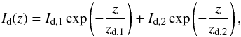 (1)where Id,1 +
Id,2 is the dust surface brightness at the
galactic midplane, and zd,1 and zd,2 are the scale
heights of two dust components. We then convolved this general vertical profile with the PSF
of each instrument used in our analysis and compared the resulting profiles with
observations.
(1)where Id,1 +
Id,2 is the dust surface brightness at the
galactic midplane, and zd,1 and zd,2 are the scale
heights of two dust components. We then convolved this general vertical profile with the PSF
of each instrument used in our analysis and compared the resulting profiles with
observations.
3.1. Point and “line” spread functions
For an extended object, the observed surface brightness distribution, g(i,j), is
the result of the convolution of an intrinsic surface brightness distribution,
f(i,j), with the instrument
PSF(i,j),
\nonumber\\[3mm] & =& \sum_{s \,=\, -N_i/2}^{N_i/2} \sum_{t \,=\, -N_j/2}^{N_j/2} f(s,t) \,{\rm PSF}(i-s,j-t), \end{eqnarray}](/articles/aa/full_html/2016/02/aa26950-15/aa26950-15-eq45.png) (2)where i and j are two perpendicular
directions and Ni and
Nj are the number of
pixels along these two directions, respectively. A (resolved) edge-on galaxy is a
particular case of extended emission source, where the surface brightness has a smooth
gradient along the galactic disc compared to the perpendicular direction (here defined as
i and
j
directions, respectively). Assuming that the intrinsic emission is constant along
i and
infinitely extended (or at least much more extended than the considered region), so that
(2)where i and j are two perpendicular
directions and Ni and
Nj are the number of
pixels along these two directions, respectively. A (resolved) edge-on galaxy is a
particular case of extended emission source, where the surface brightness has a smooth
gradient along the galactic disc compared to the perpendicular direction (here defined as
i and
j
directions, respectively). Assuming that the intrinsic emission is constant along
i and
infinitely extended (or at least much more extended than the considered region), so that
 , with
 any position along i, we can write:
![Mathematical equation: \begin{eqnarray} \label{eq:conv2} g(\overline{\imath},j) & = &\sum_{t \, = \, -N_j/2}^{N_j/2} f(t) \left[ \sum_{s \, =\, -N_i/2}^{N_i/2} {\rm PSF}(\overline{\imath}-s,j-t) \right]\nonumber\\[3mm] & =& \sum_{t \, =\, -N_j/2}^{N_j/2} f(t)\, {\rm LSF}(j-t) \end{eqnarray}](/articles/aa/full_html/2016/02/aa26950-15/aa26950-15-eq52.png) (3)where the “line” spread function (LSF)
(3)where the “line” spread function (LSF)
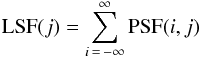 represents a vertical cut of the
two-dimensional image that results from the convolution of the instrument PSF with an
infinitely thin line. Based on the above assumptions (see Appendix A for a test on the assumed geometrical model), a vertical profile
that was extracted from the image at a position can be compared equivalently to
represents a vertical cut of the
two-dimensional image that results from the convolution of the instrument PSF with an
infinitely thin line. Based on the above assumptions (see Appendix A for a test on the assumed geometrical model), a vertical profile
that was extracted from the image at a position can be compared equivalently to
-
a profile,
 , extracted from a modelled image
obtained from the convolution of the two-dimensional intrinsic surface brightness
distribution, f(i,j), with the PSF (Eq.
(2));
, extracted from a modelled image
obtained from the convolution of the two-dimensional intrinsic surface brightness
distribution, f(i,j), with the PSF (Eq.
(2)); -
a one-dimensional model, f(j), convolved with the LSF (Eq. (3)).
The first approach was used by Bianchi & Xilouris (2011), while the second by Verstappen et al. (2013) and Hughes et al. (2014) (though without a formal demonstration of its validity). In this work we use the latter.
3.2. Spitzer and Herschel PSFs
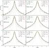 |
Fig. 2 Normalised vertical profiles for observations (black solid lines). The green dashed lines are the result of the convolution of the one-component dust emission profile with the instrument LSF while the red dashed lines are the result of convolution of the two-component dust emission profile. Normalisation values are 82.03, 48.17, 1119.47, 2023.22, 1798.00, 630.58 MJy/sr for IRAC 8, MIPS 24, PACS 70, 100, 160 and SPIRE 250 μm observed profiles, respectively. Fit results are indicated in the green and red boxes, respectively (scaleheights expressed in kpc and the intrinsic surface brightness in MJy/sr). LSF and PSF vertical profiles are illustrated with blue and orange dotted lines, respectively. |
Knowing the PSF of an instrument with a good precision is key to performing convolution (or deconvolution) operations on images, and we, therefore, carefully consider several details to have the best estimate of each PSF. In particular, the vertical profile of this source is resolved but its extent is comparable to the FWHM of the PSF, which therefore maks the choice of the right set of PSFs a critical issue.
Theoretical Herschel PACS PSFs are released by the PACS Instrument
Control Centre (ICC) assuming a spectral slope α = −4 in Fλ, which corresponds to
the ideal PSF that would have a point source with a very high temperature and that emits
with a blackbody spectrum, Bν(T)
(we will refer to these PSFs as A(std)). However, dust emits with a modified blackbody
spectrum,  , where β is the spectral index and
Bν(T)
is a blackbody radiation for an equilibrium temperature T. Dust in galaxies is
expected to be in thermal equilibrium at an average temperature T ~ 20 K and a
spectral index β ~
2, leading to a modification of the effective PSF. We therefore
modified the A(std) PSFs according to the dust spectrum assuming T = 20 K and
β = 2 (see
Appendix B.1 for a detailed description of the
method used). We will refer to these PSFs as A(mod).
, where β is the spectral index and
Bν(T)
is a blackbody radiation for an equilibrium temperature T. Dust in galaxies is
expected to be in thermal equilibrium at an average temperature T ~ 20 K and a
spectral index β ~
2, leading to a modification of the effective PSF. We therefore
modified the A(std) PSFs according to the dust spectrum assuming T = 20 K and
β = 2 (see
Appendix B.1 for a detailed description of the
method used). We will refer to these PSFs as A(mod).
We compared both the standard and modified PACS PSFs with observations of Vesta and Mars (point-like sources in PACS bands) and we noted relevant differences in the emission profile. For this reason, we combined these observations to have a better estimate of the observed PSF (B(std), see Appendix B.2 for details). As for the theoretical PSFs from the ICC, we modified the observed PSFs according to the dust spectrum, assuming the same temperature and β values (B(mod)).
Herschel SPIRE PSFs are released by the ICC and are obtained from scan-map data of Neptune and therefore represent empirical beam maps, A(std). Using the same method as for the PACS PSFs, we modified them according to the dust spectrum and assumed the same temperature and β values (see Appendix B.1 for details, A(mod)).
The IRAC Instrument Support Team noted that IRAC PSFs were undersampled and so they developed point response functions (PRFs) that combine the PSF information and the detector sampling. The PRFs were generated from models refined with in-flight calibration test data, which involves, a bright calibration star observed at several epochs, thus making them good estimates of the observed beam2.
Theoretical PSFs for the Spitzer MIPS camera were generated by Aniano et al. (2011), using the software STinyTim3. They assumed a blackbody source at T = 25 K and used a pixel size of 0.5′′ (we will refer to the MIPS 24 μm PSF as A(std)). As the optics are very smooth, the PSFs generated in this way match the observed PSFs with sufficient precision (MIPS Instrument Handbook).
After several tests, we define our best estimate of PSFs as A(std) for IRAC and MIPS, B(mod) for PACS, and A(mod) for SPIRE. All these PSFs cover a large dynamic range (≳106) and are defined up to large radii from the centre (>3 arcmin); thus they should not miss any faint point-source extended emission.
None of the PSFs described above were circularised so the relative orientation between PSF and image needs to be taken into account. This is achieved by rotating the PSF image so that the direction of the spacecraft Z-axis aligns with the direction of the spacecraft Z-axis on NGC 891 images (indicated by the white arrow for all images in Fig. 1). Subsequently, to obtain the LSF, for each vertical distance, pixels are summed along the direction of the galactic major axis. The LSF is always broader than the PSF because of the integrated contribution of the PSF Airy rings off the main beam (PSF and LSF would have the same FWHM, instead, if the PSF were Gaussian and circular). However, some positions along the major axis of an edge-on galaxy might be dominated by the emission of unresolved sources (such as bright star-forming regions), rather than from a more diffuse disc. The vertical profile above those regions would then appear narrower. We will discuss the impact of this issue on our analysis in Sect. 4. A vertical cut of LSFs and PSFs for all the considered instruments are shown in Fig. 2 with blue and orange dotted lines, respectively.
3.3. Vertical profile extraction and error estimation
To extract vertical profiles from observations we consider strips of (−7,+7) kpc parallel to the major axis of the
galaxy (corresponding to −2.5′,+
2.5′) from the centre of the galaxy (α = 2h22m33 0, δ = 42°20′57
 2,
J2000.0, blue cross in Fig. 1), where the radial
profile along the midplane is relatively constant (emission always larger than
~1 / 10 of the peak, see Fig. 4) in all bands that we considered. For each distance
from the midplane (the vertical step is one pixel) we then calculate the median emission
over all the pixels in the row within the specified area. Vertical profiles are normalised
to unity and shown in Fig. 2 with black solid lines.
2,
J2000.0, blue cross in Fig. 1), where the radial
profile along the midplane is relatively constant (emission always larger than
~1 / 10 of the peak, see Fig. 4) in all bands that we considered. For each distance
from the midplane (the vertical step is one pixel) we then calculate the median emission
over all the pixels in the row within the specified area. Vertical profiles are normalised
to unity and shown in Fig. 2 with black solid lines.
Dust emission scale heights (for thin and thick discs) as measured using IRAC, MIPS, PACS, and SPIRE instruments.
A careful estimation of the uncertainties is needed to make a comparison of the convolved
dust emission profile with observations. Following Ciesla
et al. (2012), Roussel (2013) and Cortese et al. (2014), we identified two main sources
of uncertainties. The first source is the instrumental noise, σinstr, based on
the error map. This noise depends on the number of scans crossing a pixel and can be
estimated using the sum in quadrature of the error map pixels in the measurement region.
The second source is from background noise, σsky, and can be estimated as
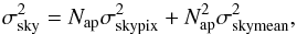 (4)where σskypix is the
rms of the fluxes in the chosen aperture4,
Nap is the number of pixels in the
aperture, and σskymean is the standard deviation of
the mean value of the sky measured in different apertures far from the galaxy. For each
vertical distance, the aperture is defined as the row of pixels upon which we calculate
the median emission (in this case from −7 kpc to +7 kpc from the galactic centre).
(4)where σskypix is the
rms of the fluxes in the chosen aperture4,
Nap is the number of pixels in the
aperture, and σskymean is the standard deviation of
the mean value of the sky measured in different apertures far from the galaxy. For each
vertical distance, the aperture is defined as the row of pixels upon which we calculate
the median emission (in this case from −7 kpc to +7 kpc from the galactic centre).
We then obtain the total uncertainty, σtot, as
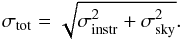 (5)We note that, since we are not comparing
images directly at different wavelengths, calibration errors are not considered here, but
will be in Sect. 5.
(5)We note that, since we are not comparing
images directly at different wavelengths, calibration errors are not considered here, but
will be in Sect. 5.
3.4. Fitting results
We consider two possibilities, a single dust component (1c), for which Id,2 = 0 in Eq.
(1) or two separated dust components
(2c). We then convolve the intrinsic vertical profile to the corresponding instrument LSF
(we use our best set of PSFs here) and used a χ2-minimisation routine to fit the
observed vertical profiles. The resulting convolved vertical profiles are shown in Fig.
2 in green (1c) and red (2c) dashed lines,
normalised to unity at the galactic midplane. Fitting parameters are indicated for the two
cases5, the intrinsic dust surface brightness is
expressed in MJy/sr, and scale heights in kpc. Both visually and from fitting parameters,
we note that the two dust component case best fit the observations for all considered
instruments. In particular,  for the two dust component case is
≲5 (with the exception of
IRAC 8 μm
data where
for the two dust component case is
≲5 (with the exception of
IRAC 8 μm
data where  ), while for the case of a single dust
component is always ≳5 times
larger. Using different sets of PSFs, the assumption of two dust components always leads
to a better fit to observations for all the considered wavelengths.
), while for the case of a single dust
component is always ≳5 times
larger. Using different sets of PSFs, the assumption of two dust components always leads
to a better fit to observations for all the considered wavelengths.
Hereafter we therefore only consider the case of two dust components. We have convolved the intrinsic vertical profile with all the PSFs described earlier, and we report the scaleheights of the thin and thick components for different PSFs and for all the considered instruments in Table 1. The errors indicated in this table result from the χ2-minimisation technique. Region X refers to a particular region in NGC 891, at a projected radial distance of hX ~ 5.6 kpc SSW from the galactic centre, where the influence from unresolved sources was estimated to be lower (see Sect. 4). Scale heights for this region are only illustrated for our best estimates of the PSFs.
While the use of standard (std) or modified (mod) PSFs does not affect the scale heights, a substantial change is achieved using A or B PSFs for PACS (see Appendix B.3 for more details). Moreover, scale heights for Region X are always greater (by more than a factor of two in some cases) than estimates integrated over the global (± 7 kpc) strip as described in Sect. 3.3.
Figure 3 shows the two scale heights (black and red symbols for thin and thick components, respectively) for our best set of PSFs. Error bars indicate the errors resulting from the χ2-minimisation technique. Results from fitting optical/NIR images with radiative transfer models are shown with green triangles (Xilouris et al. 1999). Red and black dots represent the dust scale heights for Region X.
Scale heights obtained from observations at galactic scale show a wavelength gradient for
 m for both the
thin and thick components. However, estimates from Region X show a smoother gradient for
the scale height of the thin component and an almost constant scale height for the thick
component with variations of ≲30%. The observed gradient in the scale height of the thin component
may indicate that (see discussion in Sect. 6)
m for both the
thin and thick components. However, estimates from Region X show a smoother gradient for
the scale height of the thin component and an almost constant scale height for the thick
component with variations of ≲30%. The observed gradient in the scale height of the thin component
may indicate that (see discussion in Sect. 6)
-
1.
the dust temperature quickly drops within its scale height, which leads to the dimming of the FIR emission or
-
2.
region X is also affected by the emission of point-like sources, which emit at relatively warm temperatures, and which therefore tend to reduce the effective scale height depending on the relative wavelength.
Furthermore, the scale heights of the thin component obtained from 8 and 24-μm emissions are very similar both for measurements at galactic scale and in Region X. This indicates that these estimates are affected by the presence of point sources to the same degree. On the other hand, the thick component at 24 μm is ~1.6 times more extended than at 8 μm.
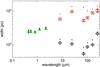 |
Fig. 3 Scale heights of the thin (black diamonds) and thick (red squares) dust components. Green triangles represent the dust scale heights as estimated by Xilouris et al. (1999). Black and red dots represent the scale heights as measured in Region X (see Sect. 4). Our best set of PSFs is used for convolution. |
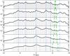 |
Fig. 4 Radial profiles for IRAC 8 μm, MIPS 24 μm, PACS 70, 100 and 160 μm and SPIRE 250 μm (from top to bottom). The position of the main peaks in emission (blue dotted lines) and the Region X (green dashed lines) are indicated. |
4. Vertical profile variation
To inspect the variability of the vertical profile across the galaxy, we subdivided the midplane into radial regions. Each region was chosen to have a radial width that is twice as large as the FWHM of the instrument PSF. Radial profiles for all considered wavelengths are shown in Fig. 4, and shaded regions indicate the radial portions into which the midplane has been divided. The position of the main peaks in emission is highlighted by the blue dotted lines.
We define Region X as the vertical strip cutting the midplane at a projected distance hX SSW from the galaxy centre. This region has been chosen as having a radial width that is twice as large as the FWHM of the instrument PSF and not to comprise any of the main emission peaks for all the wavelengths we considered. Furthermore, the continuum-subtracted Hα emission-line image of this galaxy (Fig. 10 in Howk & Savage 2000) shows that most of the galactic disc is bright in Hα, indicating the presence of several large Hii regions. However, at the position corresponding to our Region X, the Hα emission is the lowest observed in the midplane, therefore suggesting a low contamination by bright and hot dust emission from Hii regions, and make this region unique in this source. In Fig. 4 we indicate Region X with green dashed lines.
We extract the vertical profile for each of the considered regions and for all the considered wavelengths. In Fig. 5 we show the vertical profiles for PACS 100 μm as an example. The intensity of the shades of grey indicates the surface brightness of dust emission (black being the brightest region). A vertical cut of the PSF and the LSF are indicated by orange and blue lines, respectively. The convolved vertical profile obtained from fitting the observed vertical profile of the whole galaxy (−7 kpc to 7 kpc from the centre) is shown with a red dotted line, while the green dashed line indicates the convolved vertical profile that is obtained from fitting observations in Region X.
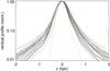 |
Fig. 5 Vertical profiles at 100 μm as measured in different radial regions. A vertical cut of the PSF (orange) and of the LSF (blue) is indicated. The vertical profile for the whole galaxy and for Region X are shown in red and green, respectively. |
Our analysis shows that there is some variation in the vertical profiles. Bright regions have a narrower vertical profile, which indicates that these regions might be dominated by isolated point sources or by a very thin disc that is not resolved in the vertical profile (see Appendix A for further details). On the contrary, in Region X, where the radial profile in the midplane is rather flat, the extracted vertical profile is close to the widest observed vertical profile. Region X is therefore affected to a low degree by the emission of unresolved sources, and for this reason, the vertical profile extracted in this region represents a better estimate of the real extent of extra-planar dust with respect to the vertical profile that is extracted at galactic scale. Scale heights of the thin and thick discs retrieved from fitting observations in Region X are indicated in Fig. 3 (see the black and red dots, respectively) and listed in Table 1.
5. Dust spectral energy distributions
By fitting the median vertical profiles of Region X for each wavelength, we can construct dust spectral energy distributions (SED) of dust for each vertical distance from the galaxy midplane. We computed the uncertainties on the surface brightness in this way: considering the parameters for Region X that are listed in Table 1, we randomly generated a large number of profiles following a Gaussian distribution centred at zd,1 and zd,2 and with the standard deviation given by the error on parameters. For each vertical distance we then computed the mean intensity and the standard deviation of the distribution, which will represent the error on the mean intensity. Furthermore, since we are comparing fluxes in different bands, we need to include the calibration errors, σcal, which are added in quadrature to the errors computed earlier. We consider a calibration uncertainty of 3% (IRAC Instrument Handbook), 4% (Bendo et al. 2012), 7% (Balog et al. 2014), and 7% (SPIRE Handbook Version 2.5) for IRAC, MIPS, PACS, and SPIRE data, respectively.
5.1. Dust modelling
For each vertical distance we fit the intrinsic spectrum from 8 μm to 250 μm using the Jones et al. (2013) dust model and the DustEM code6 to compute the dust SED. During this procedure we use the standard Mathis et al. (1983) interstellar radiation field and allow the following parameters to vary:
-
G0, a parameter that indicates the intensity of the radiation field;
-
amin, the minimum size of small grains in the model;
-
mSG/mLG, the ratio between the mass of small grains and that of large grains.
In this way we can constrain the radiation field intensity and the fraction of small grains.
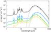 |
Fig. 6 Spectra for z = 0, 0.6, 1.5, 2.5 kpc (top to bottom). The fit using the Jones et al. (2013) dust model, is indicated with solid lines. Spectra from 70 μm to 250 μm are fit with modified blackbody radiation with fixed β = 2 (dotted lines). |
Furthermore, to have information on the average dust temperature and on its opacity, we
fit the SED from 70 μm to 250 μm to a single-temperature modified blackbody
radiation (MBB), 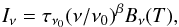 (6)where τν0 is the
optical depth at a frequency ν0 corresponding to 100 μm, β is the spectral index at
ν0 and Bν(T)
is a blackbody radiation for an equilibrium temperature T.
(6)where τν0 is the
optical depth at a frequency ν0 corresponding to 100 μm, β is the spectral index at
ν0 and Bν(T)
is a blackbody radiation for an equilibrium temperature T.
Figure 6 shows the spectra at vertical distances z = 0,0.6,1.5,2.5 kpc (from top to bottom). Solid lines represent the dust SED obtained from fitting the dust model, while dotted lines represent the fit to a modified blackbody, where fixed β = 2. The emission intensity decreases with increasing z, and the modified blackbody peak position does not follow a clear trend.
Furthermore, we find that the value of amin goes from amin = (0.40 ± 0.05) nm at the galactic disc to amin = (0.70 ± 0.05) nm at 2.5 kpc above the disc. Consequently, the mass of small grains is reduced from mSG/mLG = (6.2 ± 0.1) × 10-2 to mSG/mLG = (3.9 ± 0.1) × 10-2. This indicates that small grains are partly destroyed when moving from the galactic disc up to 2.5 kpc above it. This could suggest that dust is entrained by interstellar shocks or galactic fountains and that during coupling to the gas, small grains are partly eroded because of the high relative velocity with the gas. Similar results have been observed in supernova remnants in the LMC (Borkowski et al. 2006; Williams et al. 2006) and obtained from theoretical modelling (Micelotta et al. 2010; Bocchio et al. 2014).
As further analysis, we include collisional heating of dust because of the presence of
the hot halo gas, with an updated version of the DustEM code as described by Bocchio et al. (2013). From deep Chandra
data, Hodges-Kluck & Bregman (2013)
found hot halo gas at a temperature Tgas ~ 0.2 keV following a vertical
exponential distribution  (7)where n0 ~ 6 ×
10-3 cm-3 and zhg = 5 ± 2 kpc. Large grains are not
affected by this extra source of heating and their temperature is completely determined by
the intensity of the radiation field. On the other hand, small grains reach high
temperatures and will emit more than if only heated by the radiation field. This leads to
amin = (0.90 ±
0.05) nm and mSG/mLG = (3.3 ± 0.1) ×
10-2 at 2.5 kpc above the disc, which supports the idea
that small grains are partly eroded when moving from the galactic plane to 2.5 kpc above
it.
(7)where n0 ~ 6 ×
10-3 cm-3 and zhg = 5 ± 2 kpc. Large grains are not
affected by this extra source of heating and their temperature is completely determined by
the intensity of the radiation field. On the other hand, small grains reach high
temperatures and will emit more than if only heated by the radiation field. This leads to
amin = (0.90 ±
0.05) nm and mSG/mLG = (3.3 ± 0.1) ×
10-2 at 2.5 kpc above the disc, which supports the idea
that small grains are partly eroded when moving from the galactic plane to 2.5 kpc above
it.
5.2. Dust temperature estimation
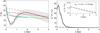 |
Fig. 7 Temperature (left panel) and
|


One of the main parameters that we obtain from fitting data to an MBB is the luminosity-weighted mean dust temperature at each vertical distance, which is shown in the left-hand panel of Fig. 7 with a black solid line. We also show the dust temperature for the thin and thick disc separately with dotted and dashed lines, respectively. The dust temperature in the thin disc drops off rapidly while the dust temperature in the thick disc stays more elevated further away from the midplane. However, the dust temperature estimation depends greatly on the scale heights obtained for the two dust components. In particular, the steep gradient in the scale height of the thin component might be affected by emission from a thin, unresolved, disc and this effect would be reflected in the temperature estimation for z ≲ 1 kpc (see discussion in Sect. 6.1).
As a comparison, exploiting the results from radiative transfer models and assuming a dust model, it is possible to calculate the resulting dust temperature. We assumed the dust optical properties and size distributions from Jones et al. (2013) and, we use different radiation fields, specific for this galaxy, which were obtained from radiative transfer models from the literature:
-
Bocchio et al. (2012), RT3.
Using the DustEM code we then compute the dust SED and, fitting it to an MBB for λ ≳ 70 μm, we estimate the average temperature of the large grains.
The resulting dust temperature profiles are shown in Fig. 7 for RT1 (blue line), RT2 (red line) and RT3 (green line). It should be noted that, using the Draine & Li (2007) dust model (as originally used in RT1 and RT2) instead of the one by Jones et al. (2013), the temperature is systematically higher, but the difference between the two estimates is never higher than ~1 K, and that temperature profiles follow the same trends.
The dust temperature profile given by our fit follows the same trend as that estimated using only radiative transfer models for z ≳ 1.5 kpc, where the dust temperature is dominated by the thick dust component. On the contrary, the dust temperature of the thin dust component drops off more quickly than expected, reaching T ~ 16 K at ~0.5 kpc from the galactic plane. In the case of Region X not being affected by the emission of unresolved sources, this discrepancy would require the presence of two distinct heating sources for the two dust component (see Sect. 6.2).
5.3. Optical depth estimation
The other main parameter, obtained from the fitting procedure, is the optical depth at
100 μm at
projected radial distance hX,
 . To compare this parameter with the
face-on central optical depth in the B-band,
. To compare this parameter with the
face-on central optical depth in the B-band,  , from the three radiative transfer models
cited above (i.e. RT1, RT2, and RT3) we first convert τ100 in
τB using the
τ100/τB ≃
7.5 × 10⁻⁴ from Jones et al.
(2013) dust model. A similar ratio, τ100/τB ≃
1.0 × 10⁻³, is assumed by the Draine & Li (2007) dust model. The profile of
, from the three radiative transfer models
cited above (i.e. RT1, RT2, and RT3) we first convert τ100 in
τB using the
τ100/τB ≃
7.5 × 10⁻⁴ from Jones et al.
(2013) dust model. A similar ratio, τ100/τB ≃
1.0 × 10⁻³, is assumed by the Draine & Li (2007) dust model. The profile of
 (h = hX) is shown in
the right-hand panel of Fig. 7 with black lines, and
contributions from the thin and thick dust components are indicated with dotted and dashed
lines, respectively. A zoom of the thick component is illustrated in the inset.
(h = hX) is shown in
the right-hand panel of Fig. 7 with black lines, and
contributions from the thin and thick dust components are indicated with dotted and dashed
lines, respectively. A zoom of the thick component is illustrated in the inset.
Then, following Kylafis & Bahcall (1987), the
conversion between the τe(h =
hX) and τf,c is given by
 (8)We see from Fig. 7 that
  at the midplane. Using the conversion
factor from Eq. (8) we then obtain
at the midplane. Using the conversion
factor from Eq. (8) we then obtain
 . The typical values of
 for radiative transfer models of this
galaxy are about a factor two higher:
for radiative transfer models of this
galaxy are about a factor two higher:  for Seon
et al. (2014) and Bianchi & Xilouris
(2011) and
for Seon
et al. (2014) and Bianchi & Xilouris
(2011) and  for Popescu et al. (2011).
We also performed a fit of the optical depth profile to an exponential function of the
form:  (9)This fit gives a scale height of
zd,2 = (1.44 ±
0.12) kpc, corresponding to the thick dust component, which is in good
agreement with both the estimate by Burgdorf et al.
(2007), zd,2 = (1.3 ± 0.3) kpc and with that by
Seon et al. (2014), zd,2 ~ [ 1.2−2.0
] kpc. Also, we calculated that ~2–3.3% of the mass of dust is present
further than 2 kpc from the midplane, which is consistent with the estimates by Seon et al. (2014).
(9)This fit gives a scale height of
zd,2 = (1.44 ±
0.12) kpc, corresponding to the thick dust component, which is in good
agreement with both the estimate by Burgdorf et al.
(2007), zd,2 = (1.3 ± 0.3) kpc and with that by
Seon et al. (2014), zd,2 ~ [ 1.2−2.0
] kpc. Also, we calculated that ~2–3.3% of the mass of dust is present
further than 2 kpc from the midplane, which is consistent with the estimates by Seon et al. (2014).
Finally, we compare the value of AV as a function of the vertical distance with the average value observed by Ménard et al. (2010) from halo extinction measurements towards distant quasars. From our observations we find AV = 0.28,0.13, and 0.064 at z = 1,2 and 3 kpc, respectively, in good agreement with values extrapolated from results by Ménard et al. (2010): AV = 0.20,0.11, and 0.076 at these three distances.
6. Discussion
As seen in Sect. 3.4, the data for NGC 891 require the presence of two dust components; this result does not depend on the choice of the PSF used in the convolution process. Furthermore, to limit the contamination from isolated point sources or from an unresolved disc, we chose to focus on Region X for the estimation of the vertical profile. Figure 3 shows that the scale height of the thick dust disc in Region X is almost constant and undergoes wavelength variations of ≲30%, while the scale height of the thin disc is always smaller than estimates by Xilouris et al. (1999), presents a gradient in wavelength, and thickens by a factor of ~4 from 70 μm to 250 μm. A similar trend is seen for all the considered PSFs (see Appendix B.3) and is therefore independent of this choice.
6.1. Thin dust component
The observed gradient in the scale height of the thin component has strong consequences on the estimation of dust temperature. The dust temperature of the thin component drops off very quickly within the first 0.5 kpc from the midplane making the optical depth estimation more difficult (see, for example, the fit to the SED at z = 0.6 kpc in Fig. 6). Furthermore, the retrieved dust temperature for z ~ 0.1−0.8 kpc is significantly lower than the dust temperature estimated from radiative transfer models.
Although our estimates of scale heights are based on observations of Region X, which is the region least affected by the presence of point sources or of an unresolved disc, even this region might suffer contamination from the emission of unresolved sources. This would result in a narrower vertical profile and this effect is likely to be wavelength-dependent, possibly leading to a gradient in scale heights similar to the one we observed.
To test this hypothesis, we add to the standard two-component intrinsic vertical profile an unresolved super-thin disc with a scale height that is fixed as equal to half of the observed image pixel size (13−45 pc). We then convolve the intrinsic vertical profile to the instrument LSF and fit the resulting profile to the observed vertical profile in Region X.
Our fits show that the relative contribution of the super-thin disc, with respect to the thin and thick components is wavelength-dependent and becomes less important going from 70 μm to 250 μm; the relative contribution of the super thin disc to the observed midplane emission ranges from ~80% at 70 μm to ~15% at 250 μm. This indicates that the spectrum of the unresolved emission from the midplane is not grey, but it peaks at wavelengths ≲70 μm, which corresponds to a dust temperature ≳40 K, consistent with the expected temperature range of dust heated by nearby hot stars. The super thin disc could thus represent the collective emission from dust heated by nearby hot stars in star-forming regions, e.g. the clumpy component of the Popescu et al. (2000a, 2011) models. Heating from star-forming regions in the galactic plane of NGC 891 was indeed found to be dominant in the shorter far-infrared (FIR) bands (Hughes et al. 2014).
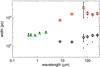 |
Fig. 8 Scale heights of the thin (black diamonds) and thick (red squares) dust components as obtained from fitting observations in Region X including the super-thin component. Green triangles represent the dust scaleheights as estimated by Xilouris et al. (1999). Black and red dots represent the scale heights as retrieved in Region X using our standard two-component model. |
In Fig. 8 we show the scale heights of the thin (black diamonds) and thick (red squares) components, obtained by fitting observations in Region X with this three-component model and comparing them with the scale heights obtained using the standard two-component model (black and red dots). The addition of the super thin component leads to a milder gradient in the scale height of the thin component for wavelengths in the range 70−250 μm. This has consequences on the estimation of dust temperature leading to a flatter temperature profile as a function of the vertical height above the midplane, which is more similar to a profile expected from RT models.
On the other hand, we find that the 8 and 24 μm data are best fit with a null contribution from the super thin disc, thus not leading to any changes in the scale height of the thin and thick components. If we admit that 70−250 μm data are affected by unresolved emission even in Region X while 8 and 24 μm data are not (or to a low extent), then the estimate of the fraction of small grains destroyed at high galactic latitudes (~2.5 kpc above the galactic disc) given in Sect. 5.1 will represent a lower limit.
However, the inclusion of a super thin disc to the standard two-component vertical profile adds complexity to the model and leads to overfitting the data. In fact, the resolution of available instruments is insufficient for probing scales of tens of parsecs at the distance of this galaxy. We therefore present the results only qualitatively from fitting a three-component model to show the consequences of the presence of unresolved sources in the midplane.
6.2. Heating sources
In the case where Region X was not highly affected by unresolved emission the big difference in dust temperature between the thin and thick components requires two different heating sources. The thin component is probably heated by the galactic radiation field, which would drop off much more quickly than expected by radiative transfer models. On the other hand, the thick dust component might be heated by the presence of a hot halo gas or from strong radiation from nearby hot evolved stars.
Assuming that the hot halo gas is distributed, as observed by Hodges-Kluck & Bregman (2013) and following the method by Bocchio et al. (2013) we computed the dust emission only in the case of collisional heating. We obtained a dust temperature Tdust = 19,18.2, and 17.4 K at z = 1,2, and 3 kpc from the midplane, respectively, which is not enough to explain the observed high dust temperature.
Another possibility comes from the strong radiation field from evolved stars present in the halo. In fact, accordingly to the model by Flores-Fajardo et al. (2011), hot low-mass evolved stars are present in the halo of NGC 891 and dominate the ionisation of the halo gas, which could possibly heat nearby dust to high temperatures. A similar source of heat was considered by Burgdorf et al. (2007) to explain the observed emission from halo dust. This model is also consistent with HST observations from Ibata et al. (2009), which show a thick stellar component with a vertical scaleheight zs = (1.44 ± 0.03) kpc.
Furthermore, observations of the Hi gas distribution from Oosterloo et al. (2007) show the presence of an Hi halo that
extends out to about 14 kpc from the midplane in the northeast, southeast, and southwest
quadrants, while a flare extending out to ~22 kpc is observed in the northwest quadrant. A few years later
Yim et al. (2011), using Very Large Array
observations, detected thin and thick Hi components. They modelled the thick
distribution with a Gaussian function with a FWHM of ~2 kpc which roughly translates into an
exponential decay with a scale height of ~1.4 kpc. Moreover, this galaxy has been mapped in the
J = 2–1 and
1–0 lines of 12CO
with the IRAM 30-m telescope by Garcia-Burillo et al.
(1992) and in the J =
1–0 line with the Nobeyama 45-m telescope by Sofue & Nakai (1993). These two teams detected a “halo” of
molecular gas  7 kpc
in radius and 2−3 kpc thick.
This component is very weak in the 1–0 line and seems to be relatively hot and not too
optically thick. This means that dust, Hi gas, molecular gas and stars follow a
similar distribution in the halo and that dust might be embedded in atomic/molecular gas
and then heated by this secondary distribution of stars.
7 kpc
in radius and 2−3 kpc thick.
This component is very weak in the 1–0 line and seems to be relatively hot and not too
optically thick. This means that dust, Hi gas, molecular gas and stars follow a
similar distribution in the halo and that dust might be embedded in atomic/molecular gas
and then heated by this secondary distribution of stars.
On the contrary, if we admit that, even in Region X there might be some contamination that results from the presence of a super-thin disc (as suggested by our three-component model analysis in Sect. 6.1), then the gradient in scale height of the thin component could be heavily smoothed. This would lead to a flatter profile in temperature, possibly similar to that of the thick component. Consequently, this scenario does not require two distinct sources of heating and the galactic radiation field, as modeled by various radiative transfer models would be sufficient to explain the high dust temperature in the halo of the galaxy.
6.3. The origin of extra-planar dust
We detected dust emission at  kpc from the galactic disc.
However, the evidence for extra-planar dust is not limited to NGC 891. Dusty clouds have
been observed in extinction up to z ~ 2 in the thick discs of the majority of
edge-on galaxies (Howk & Savage 1997, 1999, 2000;
Rossa et al. 2004; Thompson et al. 2004; Howk 2005,
2012). The optical images of these galaxies often
show filamentary structures that are perpendicular to the galactic disc, which link the
thin and thick discs. In addition, extended (up to ~6 kpc) mid-infrared aromatic feature
emission is seen around a number of galaxies (see e.g. Engelbracht et al. 2006; Irwin & Madden
2006; McCormick et al. 2013).
kpc from the galactic disc.
However, the evidence for extra-planar dust is not limited to NGC 891. Dusty clouds have
been observed in extinction up to z ~ 2 in the thick discs of the majority of
edge-on galaxies (Howk & Savage 1997, 1999, 2000;
Rossa et al. 2004; Thompson et al. 2004; Howk 2005,
2012). The optical images of these galaxies often
show filamentary structures that are perpendicular to the galactic disc, which link the
thin and thick discs. In addition, extended (up to ~6 kpc) mid-infrared aromatic feature
emission is seen around a number of galaxies (see e.g. Engelbracht et al. 2006; Irwin & Madden
2006; McCormick et al. 2013).
The presence of dust in galactic haloes can be the result of several important phenomena. We identified at least four mechanisms that possibly explain the presence of dust at these distances above the disc. 1) Dust can be expelled because of galactic fountains or stellar feedback (local winds). Observational and theoretical evidence show that small grains are partly destroyed during coupling with shocks and galactic fountains (Borkowski et al. 2006; Williams et al. 2006; Micelotta et al. 2010; Bocchio et al. 2014), in agreement with what we found. 2) Slow global winds (e.g. cosmic ray driven winds) could also explain the presence of dust in the galactic halo. These winds are slowly and continuously emitted by spiral galaxies pushing dust grains to high galactic latitudes. Also, the expansion of these winds leads to a rapid drop in the gas temperature, therefore reducing grain sputtering (Popescu et al. 2000b). 3) Another possibility comes from radiation pressure. In fact, Ferrara et al. (1991) show that this mechanism might displace dust up to several kpc from the galactic disc. 4) Finally, a significant contribution to the observed dust might come from dust formed in situ around AGB stars present in the halo (Howk 2012). However, this scenario is not very likely since it would not explain the grain erosion above the galactic midplane.
A significant amount of dust is observed even further out in the IGM around galaxies (Zaritsky 1994; Ménard et al. 2010). The thick dusty disc described here would be an interface from which dust is ejected into the IGM.
7. Summary
We have analysed deep PACS data, together with IRAC, MIPS, and SPIRE data and we detected dust emission from the halo of NGC 891. Our main findings are summarised here.
-
Dust emission at all wavelengths is best fit by a double exponential profile revealing the presence of two dust components: a thin and a thick disc.
-
The measured scale height of the thin disc shows a gradient through the FIR. It is possible to explain this by a dramatic drop in dust temperature within the thin disc scale height. Alternatively, contamination from a super thin disc may also produce this effect and reconcile the observations with standard RT models for this galaxy.
-
We obtain a precise measurement of the thick halo scaleheight, zd,2 = (1.44 ± 0.12) kpc, which agrees with previous estimates (Burgdorf et al. 2007; Kamphuis et al. 2007; Whaley et al. 2009; Seon et al. 2014).
-
We find that a non-negligible fraction (2−3.3%) of the mass of dust is located further than 2 kpc from the midplane, in accordanc with findings by Seon et al. (2014). Furthermore, the relative abundance of small grains with respect to large grains drops from mSG/mLG = (6.2 ± 0.1) × 10-2 in the galactic disc to mSG/mLG = (3.9 ± 0.1) × 10-2 at a height of ~2.5 kpc above the plane, which suggests that dust is hit by interstellar shocks or galactic fountains and entrained together with gas to a height of a few kpc from the midplane.
-
The detected halo dust component is found to have a similar extent of the atomic / molecular gas distribution and of the thick stellar disc described by Ibata et al. (2009). The thick stellar disc can therefore be a possible source of heating.
IRAC PRFs are available at http://irsa.ipac.caltech.edu/data/SPITZER/docs/irac/calibrationfiles/psfprf
MIPS PSF FITS files are available at http://www.astro.princeton.edu/~ganiano/Kernels.html
σskypix defined in this way includes not only the rms of the background sky but also possible variations of the flux because of the non-flatness of the radial profile of the galaxy at different distances from the midplane.
Hughes et al. (2014) also performed single component fits at 100, 160, and 250 μm, who find longer vertical scale lengths – by up to a few times those shown in Fig. 2 of this work. However, an inspection of the vertical profiles presented in Fig. 2 of their paper, and in particular of their LSF, suggests that the vertical scales have been accidentally multiplied by constant factors. If the factors were removed, their scalelengths would be 0.14, 0.15 and 0.23 kpc at 100, 160, and 250 μm, respectively. The values are in much better agreement with our estimates, if we also consider the different treatment of the PSF we perform in this work.
PACS and SPIRE filter transmission functions and bolometer response can be accessed from the HIPE environment.
Acknowledgments
M.B. wishes to acknowledge A. Abergel (IAS, France) and H. Roussel (IAP, France) for interesting discussions on the modelling of Herschel PSFs and in particular H. Roussel for having performed data reduction for the images of Vesta and Mars. We would like to thank the referee, C. C. Popescu, for her very helpful comments. The research leading to these results has received funding from the European Research Council under the European Union (FP/2007-2013)/ERC Grant Agreement No. 306476.
References
- Alton, P. B., Xilouris, E. M., Misiriotis, A., Dasyra, K. M., & Dumke, M. 2004, A&A, 425, 109 [NASA ADS] [CrossRef] [EDP Sciences] [Google Scholar]
- Aniano, G., Draine, B. T., Gordon, K. D., & Sandstrom, K. 2011, PASP, 123, 1218 [NASA ADS] [CrossRef] [Google Scholar]
- Baes, M., Fritz, J., Gadotti, D. A., et al. 2010, A&A, 518, L39 [NASA ADS] [CrossRef] [EDP Sciences] [Google Scholar]
- Balog, Z., Muzerolle, J., Flaherty, K., et al. 2014, ApJ, 789, L38 [NASA ADS] [CrossRef] [Google Scholar]
- Bendo, G. J., Galliano, F., & Madden, S. C. 2012, MNRAS, 423, 197 [NASA ADS] [CrossRef] [Google Scholar]
- Bianchi, S. 2007, A&A, 471, 765 [NASA ADS] [CrossRef] [EDP Sciences] [Google Scholar]
- Bianchi, S. 2008, A&A, 490, 461 [NASA ADS] [CrossRef] [EDP Sciences] [Google Scholar]
- Bianchi, S., & Xilouris, E. M. 2011, A&A, 531, L11 [NASA ADS] [CrossRef] [EDP Sciences] [Google Scholar]
- Bocchio, M. 2014, Ph.D. Thesis, Université Paris Sud [Google Scholar]
- Bocchio, M., Micelotta, E. R., Gautier, A.-L., & Jones, A. P. 2012, A&A, 545, A124 [NASA ADS] [CrossRef] [EDP Sciences] [Google Scholar]
- Bocchio, M., Jones, A. P., Verstraete, L., et al. 2013, A&A, 556, A6 [NASA ADS] [CrossRef] [EDP Sciences] [Google Scholar]
- Bocchio, M., Jones, A. P., & Slavin, J. D. 2014, A&A, 570, A32 [NASA ADS] [CrossRef] [EDP Sciences] [Google Scholar]
- Borkowski, K. J., Williams, B. J., Reynolds, S. P., et al. 2006, ApJ, 642, L141 [NASA ADS] [CrossRef] [Google Scholar]
- Burgdorf, M., Ashby, M. L. N., & Williams, R. 2007, ApJ, 668, 918 [NASA ADS] [CrossRef] [Google Scholar]
- Ciesla, L., Boselli, A., Smith, M. W. L., et al. 2012, A&A, 543, A161 [NASA ADS] [CrossRef] [EDP Sciences] [Google Scholar]
- Cortese, L., Fritz, J., Bianchi, S., et al. 2014, MNRAS, 440, 942 [NASA ADS] [CrossRef] [Google Scholar]
- De Geyter, G., Baes, M., Camps, P., et al. 2014, MNRAS, 441, 869 [NASA ADS] [CrossRef] [Google Scholar]
- De Looze, I., Baes, M., Bendo, G. J., et al. 2012, MNRAS, 427, 2797 [NASA ADS] [CrossRef] [Google Scholar]
- Draine, B. T., & Li, A. 2007, ApJ, 657, 810 [NASA ADS] [CrossRef] [Google Scholar]
- Ebert, D. S., Musgrave, F. K., Peachey, D., Perlin, K., & Worley, S. 2002, Texturing and Modeling, 3rd edn. (Morgan Kaufmann) [Google Scholar]
- Engelbracht, C. W., Kundurthy, P., Gordon, K. D., et al. 2006, ApJ, 642, L127 [NASA ADS] [CrossRef] [Google Scholar]
- Ferrara, A., Ferrini, F., Barsella, B., & Franco, J. 1991, ApJ, 381, 137 [NASA ADS] [CrossRef] [Google Scholar]
- Flores-Fajardo, N., Morisset, C., Stasińska, G., & Binette, L. 2011, MNRAS, 415, 2182 [NASA ADS] [CrossRef] [Google Scholar]
- Garcia-Burillo, S., Guelin, M., Cernicharo, J., & Dahlem, M. 1992, A&A, 266, 21 [NASA ADS] [Google Scholar]
- Griffin, M. J., Abergel, A., Abreu, A., et al. 2010, A&A, 518, L3 [Google Scholar]
- Helou, G., Roussel, H., Appleton, P., et al. 2004, ApJS, 154, 253 [NASA ADS] [CrossRef] [MathSciNet] [Google Scholar]
- Hodges-Kluck, E. J., & Bregman, J. N. 2013, ApJ, 762, 12 [NASA ADS] [CrossRef] [Google Scholar]
- Hodges-Kluck, E., & Bregman, J. N. 2014, ApJ, 789, 131 [NASA ADS] [CrossRef] [Google Scholar]
- Howk, J. C. 2005, in Extra-Planar Gas, ed. R. Braun, ASP Conf. Ser., 331, 287 [Google Scholar]
- Howk, J. C. 2012, in EAS Pub. Ser. 56, ed. M. A. de Avillez, 291 [Google Scholar]
- Howk, J. C., & Savage, B. D. 1997, AJ, 114, 2463 [NASA ADS] [CrossRef] [Google Scholar]
- Howk, J. C., & Savage, B. D. 1999, AJ, 117, 2077 [NASA ADS] [CrossRef] [Google Scholar]
- Howk, J. C., & Savage, B. D. 2000, AJ, 119, 644 [NASA ADS] [CrossRef] [Google Scholar]
- Hughes, T. M., Baes, M., Fritz, J., et al. 2014, A&A, 565, A4 [NASA ADS] [CrossRef] [EDP Sciences] [Google Scholar]
- Ibata, R., Mouhcine, M., & Rejkuba, M. 2009, MNRAS, 395, 126 [NASA ADS] [CrossRef] [Google Scholar]
- Irwin, J. A., & Madden, S. C. 2006, A&A, 445, 123 [NASA ADS] [CrossRef] [EDP Sciences] [MathSciNet] [Google Scholar]
- Jones, A. P., Fanciullo, L., Köhler, M., et al. 2013, A&A, 558, A62 [NASA ADS] [CrossRef] [EDP Sciences] [Google Scholar]
- Kamphuis, P., Holwerda, B. W., Allen, R. J., Peletier, R. F., & van der Kruit, P. C. 2007, A&A, 471, L1 [NASA ADS] [CrossRef] [EDP Sciences] [Google Scholar]
- Kylafis, N. D., & Bahcall, J. N. 1987, ApJ, 317, 637 [NASA ADS] [CrossRef] [Google Scholar]
- Makovoz, D., & Marleau, F. R. 2005, PASP, 117, 1113 [NASA ADS] [CrossRef] [Google Scholar]
- Mathis, J. S., Mezger, P. G., & Panagia, N. 1983, A&A, 128, 212 [NASA ADS] [Google Scholar]
- McCormick, A., Veilleux, S., & Rupke, D. S. N. 2013, ApJ, 774, 126 [NASA ADS] [CrossRef] [Google Scholar]
- Ménard, B., Scranton, R., Fukugita, M., & Richards, G. 2010, MNRAS, 405, 1025 [NASA ADS] [Google Scholar]
- Micelotta, E. R., Jones, A. P., & Tielens, A. G. G. M. 2010, A&A, 510, A36 [NASA ADS] [CrossRef] [EDP Sciences] [Google Scholar]
- Oosterloo, T., Fraternali, F., & Sancisi, R. 2007, AJ, 134, 1019 [NASA ADS] [CrossRef] [Google Scholar]
- Ott, S. 2010, in Astronomical Data Analysis Software and Systems XIX, eds. Y. Mizumoto, K.-I. Morita, & M. Ohishi, ASP Conf. Ser., 434, 139 [Google Scholar]
- Pilbratt, G. L., Riedinger, J. R., Passvogel, T., et al. 2010, A&A, 518, L1 [CrossRef] [EDP Sciences] [Google Scholar]
- Poglitsch, A., Waelkens, C., Geis, N., et al. 2010, A&A, 518, L2 [NASA ADS] [CrossRef] [EDP Sciences] [Google Scholar]
- Popescu, C. C., & Tuffs, R. J. 2013, MNRAS, 436, 1302 [NASA ADS] [CrossRef] [Google Scholar]
- Popescu, C. C., Misiriotis, A., Kylafis, N. D., Tuffs, R. J., & Fischera, J. 2000a, A&A, 362, 138 [NASA ADS] [Google Scholar]
- Popescu, C. C., Tuffs, R. J., Fischera, J., & Völk, H. 2000b, A&A, 354, 480 [NASA ADS] [Google Scholar]
- Popescu, C. C., Tuffs, R. J., Dopita, M. A., et al. 2011, A&A, 527, A109 [NASA ADS] [CrossRef] [EDP Sciences] [Google Scholar]
- Rossa, J., Dettmar, R.-J., Walterbos, R. A. M., & Norman, C. A. 2004, AJ, 128, 674 [NASA ADS] [CrossRef] [Google Scholar]
- Roussel, H. 2013, PASP, 125, 1126 [Google Scholar]
- Seon, K.-I., & Witt, A. N. 2012, in IAU Symp. 284, eds. R. J. Tuffs, & C. C. Popescu, 135 [Google Scholar]
- Seon, K.-i.,Witt, A. N., Shinn, J.-H., & Kim, I.-J. 2014, ApJ, 785, L18 [NASA ADS] [CrossRef] [Google Scholar]
- Sofue, Y., & Nakai, N. 1993, PASJ, 45, 139 [NASA ADS] [Google Scholar]
- Strickland, D. K., Heckman, T. M., Colbert, E. J. M., Hoopes, C. G., & Weaver, K. A. 2004, ApJS, 151, 193 [NASA ADS] [CrossRef] [Google Scholar]
- Thompson, T. W. J., Howk, J. C., & Savage, B. D. 2004, AJ, 128, 662 [NASA ADS] [CrossRef] [Google Scholar]
- Verstappen, J., Fritz, J., Baes, M., et al. 2013, A&A, 556, A54 [NASA ADS] [CrossRef] [EDP Sciences] [Google Scholar]
- Whaley, C. H., Irwin, J. A., Madden, S. C., Galliano, F., & Bendo, G. J. 2009, MNRAS, 395, 97 [NASA ADS] [CrossRef] [Google Scholar]
- Williams, B. J., Borkowski, K. J., Reynolds, S. P., et al. 2006, ApJ, 652, L33 [NASA ADS] [CrossRef] [Google Scholar]
- Xilouris, E. M., Kylafis, N. D., Papamastorakis, J., Paleologou, E. V., & Haerendel, G. 1997, A&A, 325, 135 [NASA ADS] [Google Scholar]
- Xilouris, E. M., Alton, P. B., Davies, J. I., et al. 1998, A&A, 331, 894 [NASA ADS] [Google Scholar]
- Xilouris, E. M., Byun, Y. I., Kylafis, N. D., Paleologou, E. V., & Papamastorakis, J. 1999, A&A, 344, 868 [NASA ADS] [Google Scholar]
- Yim, K., Wong, T., Howk, J. C., & van der Hulst, J. M. 2011, AJ, 141, 48 [NASA ADS] [CrossRef] [Google Scholar]
- Zaritsky, D. 1994, AJ, 108, 1619 [NASA ADS] [CrossRef] [Google Scholar]
Appendix A: A simple geometrical model
For our analysis we considered strips of −2.5′, + 2.5′ from the centre of the galaxy and parallel to its major axis. In this region the radial profile is relatively constant (emission always larger than ~1 / 10 of the peak) and we therefore considered the median emission to compute the vertical profile of the galaxy. In this appendix, we use a simple geometrical model to show the general validity of our approach and study the bias in the estimates induced by geometrical components that we did not account for in the fitting.
As an example, we consider PACS 100 μm data throughout this section. We construct an array with a pixel size equal to the corresponding instrument pixel size (i.e. 1′′) with flat null background. We perform a fit to the radial emission profile and assume it as the radial profile of the intrinsic emission distribution. We use the intrinsic vertical profile that was extracted in Region X (see Sect. 3.4, zd,1 = 0.114 kpc and zd,2 = 1.02 kpc) as an estimate of the real vertical profile and we added this to all the pixels around the midplane. The simple model constructed in this way is then smoothed to the instrument resolution, which convolves it to the corresponding PSF (the B(mod) PSF for PACS 100 μm), and adjusted to match the observed surface brightness.
We extract vertical profiles by averaging over the whole galactic disc and in Region X. In Fig. A.1 we show the vertical profile extracted in Region X from our model and compare it to the observed vertical profile from Region X. We then consider a two-component intrinsic exponential profile (Eq. (1)), convolve it with the instrument LSF and fit it to the vertical profile of the convolved model (as in Sect. 3.4). The resulting profile is illustrated by the green dashed line in Fig. A.1 and the parameters retrieved from the fit are reported as case α in Table A.1. The scale height of the thin and thick components for both regions are compatible with those used to construct our simple geometrical model. The compatibility between these results demonstrates that the assumption of a flat radial profile does not introduce any systematic error in the estimation of the vertical scale heights.
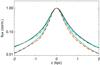 |
Fig. A.1 Normalised vertical profiles for PACS 100 μm. Blue and black solid lines refer to the observed profiles at galactic scale and for Region X, respectively. Cyan and orange solid lines represent the vertical profiles obtained from our simple geometrical model without (case α) and with (case β) a super thin disc included, respectively, while green and red dashed lines indicate the results of the fit in the two cases. |
Scale heights of the thin and thick components as extracted (at galactic scale and in Region X) from observations (obs.) and from our geometrical model.
However, this simple model is not able to reproduce the discrepancy in scale height fitting observations at galactic scale or when only considering Region X. This could be because of unresolved sources that were not accounted for in our fitting procedure (see Sects. 4 and 6.1). To test this hypothesis, we made two simple tests.
In the first test, we include a few (5) isolated point sources along the galactic plane, to simulate the main features in the observed surface brightness distribution. These features could represent inhomogeneities in the disc resulting from, for example, spiral arms seen in projection (see the discussion in Bianchi & Xilouris 2011). Being point-like, their vertical profile would follow that of a PSF, and this would make the average profile decline faster than in the case of two diffuse discs. The intensity of the point sources (modelled as bright pixels) and of the diffuse discs were scaled to match the observed average profile, and an average profile was extracted from the model as we have done before. Though the new profile (not shown) is narrower than the profile for Region X, it is very close to it and far from the observed averaged profile. Thus, isolated point sources are not likely to be the main cause of the discrepancy.
In a second test, we assume that half of the emission in the midplane comes from a very thin diffuse disc which is not resolved vertically (and thus has a vertical profile similar to that of the LSF). This is analogous to dividing the intrinsic profile by a factor two for all the pixels which are not in the midplane. An exception is made for the pixels around Region X where no bright source is added. We then convolve this model with the instrument PSF and adjust the normalisation to the observed surface brightness. The vertical profile at galactic scale of the convolved model is shown in Fig. A.1 and compared to the observed vertical profile at galactic scale. With the same method used above, the scale height of the thin and thick components are retrieved from fitting our convolved model. The resulting vertical profile is shown in Fig. A.1 and fitting parameters are reported in Table A.1 (case β). The inclusion of an unresolved disc reduces the scale height of both the thin and thick components, which leads to a good agreement between the convolved and observed vertical profiles at galactic scale. Thus, the presence of a super thin disc can explain the discrepancy between the vertical profiles extracted from observations at galactic scale and in Region X.
We note that the scale height of the thin and thick components retrieved from fitting our convolved model in Region X are not affected by the inclusion of unresolved sources along the midplane (see Table A.1; case β, Region X). However, this does not imply that we can exclude that part of the emission from the midplane of Region X, which is actually due to the presence of unresolved sources. In fact, this represents a scenario that we are unable to test with this simple geometrical model.
Appendix B: Beyond “standard” Herschel PSFs
In this work we attempt to take into account the major effects that could modify the PACS and SPIRE PSFs. In particular, we studied the variations induced by colour corrections (B.1), we derived a new set of “observed” PSFs for PACS (B.2), and finally tested the impact of these modifications on the derived vertical scale heights (B.3).
Appendix B.1: PSF modification according to the source spectrum
The effective frequency, νeff, of an instrument equipped with a narrowband filter corresponds to the frequency at the centre of the filter. For larger filters, νeff depends on the spectrum of the observed source and therefore the instrument PSF shrinks or stretches according to the source spectrum. In the latter case, a PSF estimated from observations of an astronomical object is only valid if the source that we observe has a similar spectrum to that of the object used for the PSF characterisation. However, the spectrum of an asteroid or a planet can be very different from the dust emission spectrum. For this reason we modified the PACS and SPIRE PSFs according to the typical dust temperature and β values.
Following the SPIRE Handbook (2014), a PSF depends on the frequency of the observed
source as 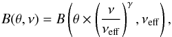 (B.1)where θ is the radial distance
from the centre, ν is the source frequency, νeff is the
effective frequency for which the PSF has been estimated, and γ is a parameter which
takes into account the slope of the spectrum within a given band (γ = −1 for an ideal
telescope).
(B.1)where θ is the radial distance
from the centre, ν is the source frequency, νeff is the
effective frequency for which the PSF has been estimated, and γ is a parameter which
takes into account the slope of the spectrum within a given band (γ = −1 for an ideal
telescope).
The SPIRE ICC provides values of γ and νeff for all SPIRE bands, in particular γ = −0.85 and νeff = 1215 GHz for SPIRE 250 μm.
For PACS bands we assume γ
= −1 and we estimate νeff from the spectrum of Vesta and
Mars as follows: 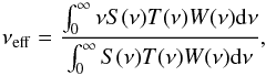 (B.2)where S(ν) is
the source of the object used for the estimation of the PSF, T(ν) is
the transmission function, and W(ν) the bolometer response7.
(B.2)where S(ν) is
the source of the object used for the estimation of the PSF, T(ν) is
the transmission function, and W(ν) the bolometer response7.
Finally we compute the PSF for a given spectrum, S′(ν) of
the object that we want to observe (i.e. dust typically at T = 20 K and
β ~
2): 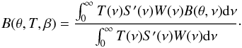 (B.3)For a more complete description of the
method used, see Bocchio (2014).
(B.3)For a more complete description of the
method used, see Bocchio (2014).
In Fig. B.1 we show PACS 70, 100, and 160 μm and SPIRE 250 μm PSFs for the standard case and modified according to the typical dust emission spectrum. Here, the “standard” PSFs for PACS are B (std), while for SPIRE these are A (std). We note that variations are never more relevant than 1% level for all wavelengths.
Given the lack of information on the IRAC and MIPS monochromatic PSFs, and given the low impact of the colour corrections for PACS and SPIRE PSFs, we do not perform this work for Spitzer PSFs.
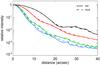 |
Fig. B.1 PACS 70, 100, and 160 μm (blue, green, and red lines, respectively) and SPIRE 250 μm (black lines) PSFs, standard and modified, assuming Tdust = 20 K and βdust = 2. |
Appendix B.2: PACS PSFs estimation from observations
To obtain a good estimate of an instrument PSF it is necessary to have information both on its core and on faint structures in the outskirts. However, this involves a wide range in intensity, and observations of a single object are often not sufficient to properly characterise a PSF.
The PACS ICC provides an optical model for the instrument PSF taking into account aberrations of the real telescope (“as built” PSF8).
We use observations of an asteroid, Vesta, and a planet, Mars, to compare the observed PSF with that modeled by the ICC. Vesta is a sufficiently faint object not to lead to any saturation or non-linear behaviour of the central pixels, which therefore allows for a good estimate of the core of the PSF. On the other hand, Mars is much brighter and leads to the complete saturation of the central pixels, but gives much more information on the PSF faint wings. The combination of these observations can thus lead to an accurate estimate of the PSF.
Observations of Vesta (ObsID: 1342195472, 1342195473 for 70 μm, 1342195476, 1342195477 for 100 μm and 1342195472, 1342195473, 1342195476, 1342195477 for 160 μm) and Mars (ObsID: 1342231157 – 1342231160 for 70 μm, 1342231161 – 1342231164 for 100 μm and 1342231157 – 1342231164 for 160 μm) were reduced following the same method as described in Sect. 2.
First, all the images have been rotated in such a way to obtain the Z-axis of the telescope during observations pointing upward. Then, we removed an average background flux for all the images that was computed in regions sufficiently far from the source. We normalised the images of Vesta to unity and rescaled the images of Mars to have the same flux in an intermediate region between the core and the outskirts of the PSF.
The average radial profiles of Vesta and Mars for PACS 70 μm are shown in Fig. B.2. The inset illustrates the ratio between the flux of Vesta and Mars as a function of the distance from the PSF centre. We note that in a region close to the centre (Region 1), the radial profile extracted from Mars does not follow that of Vesta because of saturation / non-linear issues, while at distances ≳70′′ (Region 3) the Vesta profile is not detected at a significant level. At intermediate distances (Region 2, from x1 ~ 20′′ to x2 ~ 50′′) the ratio is close to unity. As an estimate of the PSF we use Vesta observations in Region 1, Mars observations in Region 3 and the average value between the two for Region 2. We performed the same operation for PACS 100 and 160 μm, using x1 = 30 and x2 = 50 for PACS 100 μm and x1 = 40 and x2 = 70 for PACS 160 μm.
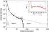 |
Fig. B.2 Radial profiles of Vesta (black solid line) and Mars (black dotted line) observations at 70 μm. In the inset, the ratio between the Vesta and Mars profiles is shown (red solid line). Regions are indicated (see text for details). |
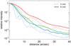 |
Fig. B.3 PSF radial profiles, as estimated from observations (solid lines) and modeled by the ICC (dotted lines) for PACS 70 μm (blue lines), 100 μm (green lines), and 160 μm (red lines). |
To obtain a smooth PSF in x1 and x2, we adopt
the following smooth step function (Ebert et al.
2002): 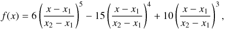 (B.4)which has zero first and second order
derivatives at the boundaries x1 and x2.
(B.4)which has zero first and second order
derivatives at the boundaries x1 and x2.
In Fig. B.3 we show radial profiles of the PACS PSFs as released by the ICC and obtained in this way. Differences are evident at all wavelengths and distances. In particular, ICC PSFs are systematically narrower than those we obtained from observations by 10–30%.
Appendix B.3: Scale heights assuming different PSFs
With the method described in Sect. 3 we estimated the scale height of the dust emission profile at different wavelengths. The instrument PSF plays a key role in this calculation. In Fig. B.4 we show the scale heights as retrieved from the fitting procedure using the different PSFs we considered in the main text. We note that the effect of modifying the PSF according to the observed source spectrum has no relevant effect on the estimation of the scale height, which reflects the weak effect on the PSF (see Sect. B.1). On the contrary, passing from the “as built” PACS PSF (A) to the one that is estimated from observations (B) affects the dust scale height significantly.
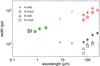 |
Fig. B.4 Scale heights of the thin (black symbols) and thick (red symbols) dust components, assuming different PSFs. Green squares represent the dust scaleheights as estimated by Xilouris et al. (1999). |
All Tables
Dust emission scale heights (for thin and thick discs) as measured using IRAC, MIPS, PACS, and SPIRE instruments.
Scale heights of the thin and thick components as extracted (at galactic scale and in Region X) from observations (obs.) and from our geometrical model.
All Figures
|
Fig. 1 From top to bottom: IRAC 8 μm (after stellar
subtraction), MIPS 24 μm, PACS 70 μm (left
column) and PACS 100 and 160 μm and SPIRE 250 μm (right
column) images of NGC 891. Each panel shows an area of ~14′ × 7′ centred on the galaxy’s
radio continuum coordinates α = 2h22m33 |
| In the text | |
|
Fig. 2 Normalised vertical profiles for observations (black solid lines). The green dashed lines are the result of the convolution of the one-component dust emission profile with the instrument LSF while the red dashed lines are the result of convolution of the two-component dust emission profile. Normalisation values are 82.03, 48.17, 1119.47, 2023.22, 1798.00, 630.58 MJy/sr for IRAC 8, MIPS 24, PACS 70, 100, 160 and SPIRE 250 μm observed profiles, respectively. Fit results are indicated in the green and red boxes, respectively (scaleheights expressed in kpc and the intrinsic surface brightness in MJy/sr). LSF and PSF vertical profiles are illustrated with blue and orange dotted lines, respectively. |
| In the text | |
|
Fig. 3 Scale heights of the thin (black diamonds) and thick (red squares) dust components. Green triangles represent the dust scale heights as estimated by Xilouris et al. (1999). Black and red dots represent the scale heights as measured in Region X (see Sect. 4). Our best set of PSFs is used for convolution. |
| In the text | |
|
Fig. 4 Radial profiles for IRAC 8 μm, MIPS 24 μm, PACS 70, 100 and 160 μm and SPIRE 250 μm (from top to bottom). The position of the main peaks in emission (blue dotted lines) and the Region X (green dashed lines) are indicated. |
| In the text | |
|
Fig. 5 Vertical profiles at 100 μm as measured in different radial regions. A vertical cut of the PSF (orange) and of the LSF (blue) is indicated. The vertical profile for the whole galaxy and for Region X are shown in red and green, respectively. |
| In the text | |
|
Fig. 6 Spectra for z = 0, 0.6, 1.5, 2.5 kpc (top to bottom). The fit using the Jones et al. (2013) dust model, is indicated with solid lines. Spectra from 70 μm to 250 μm are fit with modified blackbody radiation with fixed β = 2 (dotted lines). |
| In the text | |
|
Fig. 7 Temperature (left panel) and
|
| In the text | |
|
Fig. 8 Scale heights of the thin (black diamonds) and thick (red squares) dust components as obtained from fitting observations in Region X including the super-thin component. Green triangles represent the dust scaleheights as estimated by Xilouris et al. (1999). Black and red dots represent the scale heights as retrieved in Region X using our standard two-component model. |
| In the text | |
|
Fig. A.1 Normalised vertical profiles for PACS 100 μm. Blue and black solid lines refer to the observed profiles at galactic scale and for Region X, respectively. Cyan and orange solid lines represent the vertical profiles obtained from our simple geometrical model without (case α) and with (case β) a super thin disc included, respectively, while green and red dashed lines indicate the results of the fit in the two cases. |
| In the text | |
|
Fig. B.1 PACS 70, 100, and 160 μm (blue, green, and red lines, respectively) and SPIRE 250 μm (black lines) PSFs, standard and modified, assuming Tdust = 20 K and βdust = 2. |
| In the text | |
|
Fig. B.2 Radial profiles of Vesta (black solid line) and Mars (black dotted line) observations at 70 μm. In the inset, the ratio between the Vesta and Mars profiles is shown (red solid line). Regions are indicated (see text for details). |
| In the text | |
|
Fig. B.3 PSF radial profiles, as estimated from observations (solid lines) and modeled by the ICC (dotted lines) for PACS 70 μm (blue lines), 100 μm (green lines), and 160 μm (red lines). |
| In the text | |
|
Fig. B.4 Scale heights of the thin (black symbols) and thick (red symbols) dust components, assuming different PSFs. Green squares represent the dust scaleheights as estimated by Xilouris et al. (1999). |
| In the text | |
Current usage metrics show cumulative count of Article Views (full-text article views including HTML views, PDF and ePub downloads, according to the available data) and Abstracts Views on Vision4Press platform.
Data correspond to usage on the plateform after 2015. The current usage metrics is available 48-96 hours after online publication and is updated daily on week days.
Initial download of the metrics may take a while.