| Issue |
A&A
Volume 586, February 2016
|
|
|---|---|---|
| Article Number | A128 | |
| Number of page(s) | 20 | |
| Section | Interstellar and circumstellar matter | |
| DOI | https://doi.org/10.1051/0004-6361/201526781 | |
| Published online | 05 February 2016 | |
Ortho-to-para ratio of NH2
Herschel-HIFI observations of ortho- and para-NH2 rotational transitions towards W31C, W49N, W51, and G34.3+0.1⋆
1 Chalmers University of Technology, Department of Earth and Space Sciences, Onsala Space Observatory, 439 92 Onsala, Sweden
e-mail: carina.persson@chalmers.se
2 Department of Chemistry, University of Virginia, McCormick Road, Charlottesville, VA 22904, USA
3 Department of Physics & Astronomy, Siena College, Loudonville, NY 12211, USA
4 Université Grenoble Alpes and CNRS, IPAG, 38000 Grenoble, France
5 LERMA, Observatoire de Paris, PSL Research University, CNRS, Sorbonne Universités, UPMC Univ. Paris 06, École normale supérieure, 75005 Paris, France
6 LERMA, Observatoire de Paris, PSL Research University, CNRS, Sorbonne Universités, UPMC Univ. Paris 06, 75014 Paris, France
7 Max-Planck-Institut für Radioastronomie, Auf dem Hügel 69, 53121 Bonn, Germany
Received: 18 June 2015
Accepted: 30 November 2015
We have used the Herschel-HIFI instrument to observe the two nuclear spin symmetries of amidogen (NH2) towards the high-mass star-forming regions W31C (G10.6−0.4), W49N (G43.2−0.1), W51 (G49.5−0.4), and G34.3+0.1. The aim is to investigate the ratio of nuclear spin types, the ortho-to-para ratio (OPR) of NH2 in the translucent interstellar gas, where it is traced by the line-of-sight absorption, and in the envelopes that surround the hot cores. The HIFI instrument allows spectrally resolved observations of NH2 that show a complicated pattern of hyperfine structure components in all its rotational transitions. The excited NH2 transitions were used to construct radiative transfer models of the hot cores and surrounding envelopes to investigate the excitation and possible emission of the ground-state rotational transitions of ortho-NH2NKa,KcJ = 11,1 3/2–00,0 1/2 (953 GHz) and para-NH2 21,2 5/2–10,1 3/2 (1444 GHz) used in the OPR calculations. Our best estimate of the average OPR in the envelopes lie above the high-temperature limit of three for W49N, specifically 3.5 with formal errors of ±0.1, but for W31C, W51, and G34.3+0.1 we find lower values of 2.5 ± 0.1, 2.7 ± 0.1, and 2.3 ± 0.1, respectively. Values this low are strictly forbidden in thermodynamical equilibrium since the OPR is expected to increase above three at low temperatures. In the translucent interstellar gas towards W31C, where the excitation effects are low, we find similar values between 2.2 ± 0.2 and 2.9 ± 0.2. In contrast, we find an OPR of 3.4 ± 0.1 in the dense and cold filament connected to W51 and also two lower limits of ≳4.2 and ≳5.0 in two other translucent gas components towards W31C and W49N. At low temperatures (T ≲ 50 K) the OPR of H2 is <10-1, far lower than the terrestrial laboratory normal value of three. In this para-enriched H2 gas, our astrochemical models can reproduce the variations of the observed OPR, both below and above the thermodynamical equilibrium value, by considering nuclear-spin gas-phase chemistry. The models suggest that values below three arise in regions with temperatures ≳20−25 K, depending on time, and values above three at lower temperatures.
Key words: ISM: abundances / ISM: molecules / astrochemistry / line: formation / molecular processes / submillimeter: ISM
© ESO, 2016
1. Introduction
The amidogen (NH2) radical is an important species in the first steps of reaction chains in the nitrogen chemical network, and it is closely related to the widely observed ammonia (NH3) molecule. Observations of NH2 can be used for testing the production pathways of nitrogen-bearing molecules. Despite its importance, few observations have been performed of interstellar NH2, however, since most strong transitions fall at sub-mm wavelengths, which are difficult to observe using ground-based antennas.
Each rotational transition of NH2 has a complex fine and hyperfine structure. It is a light asymmetrical rotor with two symmetry forms, which are caused by the different relative orientations of the hydrogen nuclear spins. The symmetries are believed to behave like two distinct species: ortho-NH2 (H spins parallel) and para-NH2 (H spins anti-parallel). Its energy level diagram (Fig. A.1) is similar to that of water, with the difference that NH2 has exchanged ortho and para symmetries, that is, the lowest level (00,0) is ortho. The electronic ground state is  with a net unpaired electronic spin of 1/2, which splits each NKa,Kc level with J = N ± 1/2. The nitrogen nuclei further split all levels, and the ortho-transitions also have additional splitting that is due to the net proton spin. We note that the spin degeneracy (2I + 1) makes the ortho stronger than the para lines.
The first detection of interstellar NH2 was made by van Dishoeck et al. (1993) in absorption towards Sgr B2 (M). They detected the fundamental rotational transition NKa,Kc = 11,0−10,1 of para-NH2, with three fine-structure components at 461 to 469 GHz and partially resolved hyperfine structure. The Infrared Space Observatory (ISO) was later used by Cernicharo et al. (2000), Goicoechea et al. (2004), and Polehampton et al. (2007) to observe spectrally unresolved absorption lines of both ortho- and para-NH2 towards the same source. Goicoechea et al. (2004) inferred an NH2 ortho-to-para ratio (OPR) of 3 ± 1 towards the warm and low-density envelope around Sgr B2 (M) from the observation of ortho-NH222,0−11,1 and para-NH222,1−11,0 rotationally excited far-IR lines.
During its mission lifetime 2009−2013, the Herschel Space Observatory (Pilbratt et al. 2010), with the Heterodyne Instrument for the Far-Infrared (HIFI; de Graauw et al. 2010) offered unique capabilities for observations at very high sensitivity and high spectroscopic resolution of the fundamental rotational transitions of light hydrides at THz frequencies (0.48−1.25 THz and 1.41−1.91 THz). The PRISMAS key programme (PRobing InterStellar Molecules with Absorption line Studies) targeted absorption lines along the sight-lines towards eight bright sub-millimetre-wave continuum sources using Herschel-HIFI: W31C (G10.6−0.4), W49N (G43.2−0.1), W51 (G49.5−0.4), G34.3+0.1, DR21(OH), SgrA (+50 km s-1 cloud), W28A (G005.9−0.4), and W33A. With this technique, the interstellar gas along the sight-lines can be seen in absorption, simultaneously with the hot cores that are detected through emission and absorption.
The first results and analysis of absorption lines of nitrogen hydrides (NH, NH2, and NH3) along the sight-lines towards the massive star-forming regions W31C and W49N were presented in Persson et al. (paper I, 2010) and Persson et al. (paper II, 2012). Similar average abundances with respect to the total amount of hydrogen estimated along the whole line of sight towards W31C were found in paper I for all three species, ~6 × 10⁻⁹, 3 × 10⁻⁹, and 3 × 10⁻⁹ for NH, NH2, and NH3, respectively. These abundances were, however, estimated from the ortho NH2 and NH3 symmetries using the high-temperature OPR limits of 3 and 1, respectively. In paper II, absorptions along the sight-lines towards W31C and W49N were decomposed into different velocity components. Column densities and abundances with respect to molecular hydrogen were estimated in each velocity component, and a linear correlation of ortho-NH2 and ortho-NH3 was found with a ratio of ~1.5. We also found surprisingly low OPR ammonia values, ~0.5−0.7, below the strict high-temperature limit of unity. Values as low as this are strictly forbidden in thermodynamical equilibrium, since the OPR is expected to be unity at temperatures significantly higher than 22 K, the energy difference between ortho- and para-NH3, and increase above unity at low temperatures. As suggested by Faure et al. (2013) and further developed by Le Gal et al. (2014), a low OPR is a natural consequence of chemical gas-phase reaction pathways and is consistent with nuclear spin selection rules in a para-enriched H2 gas that drive the OPR of nitrogen hydrides to values lower than the statistical limits. Their prediction for NH2, which is directly chemically related to NH3, is an OPR of ~2.0−2.8 depending on physical conditions and initial abundances. This is in contrast to the expected increase above the high-temperature limit of 3 at low temperatures.
Our aim in this paper is to investigate the behaviour of the OPR of NH2 towards four of the PRISMAS sources: W31C, W49N, G34.3+0.1 (hereafter G34.3), and W51. To do this, we use PRISMAS data and observations of additional higher excitation transitions of NH2 from our programme OT1_cpersson_1 Investigation of the nitrogen chemistry in diffuse and dense interstellar gas.
2. Observations and data reduction
The observed high-mass star-forming regions and their properties are listed in Table 1, and the Herschel observational identifications (OBSIDs) can be found in Table B.1. Towards all four sources we have observed three ortho-NH2 and one para-NH2 line (Table 2). For the spectroscopy we consulted the Cologne Database for Molecular Spectroscopy1 (CDMS; Müller et al. 2001, 2005) based on spectroscopy by Müller et al. (1999). A fifth line, the ortho 1012 GHz line, was also detected towards W31C while searching for NH+ (Persson et al. 2012). Tables B.2−B.6 list the hyperfine structure (hfs) components of all observed transitions. The observations of the 11,1−00,0 953 GHz transition towards W31C and W49N have already been presented in Papers I and II.
Source sample properties.
Observed NH2 transitions towards W31C, W49N, W51, and G34.3+0.1, resulting continuum intensities, and noise levels.
We used the dual beam switch mode and the wide band spectrometer (WBS) with a bandwidth of 4 GHz for the lower bands, and 2.5 GHz for band 6, with an effective spectral resolution of 1.1 MHz. The corresponding velocity resolution is 0.51, 0.37, and 0.23 km s-1 at 649, 907, and 1444 GHz, respectively. Two orthogonal polarisations were used in all observations. The ortho lines were observed with three different frequency settings of the local oscillator (LO), and the para line with five settings, corresponding to a change of approximately 15 km s-1 to determine the sideband origin of the lines, since HIFI uses double-sideband (DSB) receivers. No contamination from the image sideband was detected except for several lines blended with the ortho 649 GHz line in all settings towards W49N, W51, and G34, which we were unable to remove. We use these observations as upper limits of the true 649 GHz line emission in our modelling in Sect. 3.1. The ortho 953 GHz absorption along the line-of-sight gas towards W49N is contaminated by an NO emission line from the source in the same sideband, which was removed before the analysis (described in Paper II).
The recommended values for half-power beam width of the telescope and the main beam-efficiencies are listed in Table 2 and taken from the HIFI release note 20142. The in-flight performance is described by Roelfsema et al. (2012) and the calibration uncertainties are ≲9% for band 3 and ≲11% for band 6.
The data were processed using the standard Herschel interactive processing environment (HIPE3Ott 2010), version 12.1, up to level 2 providing fully calibrated DSB spectra on the  antenna temperature intensity scale where the lines are calibrated to single sideband (SSB) and the continuum to DSB. The FITS files were then exported to the spectral line software package xs4, which was used in the subsequent data reduction. All LO-tunings and both polarisations were included in the averaged noise-weighted spectra, except for a few settings of para-NH2 which suffered from severe spikes (details in Table B.1). Absorption from HCl+ has been detected at lower velocities (~40−210 km s-1) close to our observed para-NH2 line (De Luca et al. 2012). This explains why the base line seems to present undulations at these frequencies. The averaged spectra were finally convolved from the original 0.5 MHz channel separation to the effective spectral resolution of 1.1 MHz. In order to derive the OPR, we resampled the para spectra to the velocity resolution of the ortho spectra, which allows comparison of column densities in individual velocity bins.
The resulting noise and SSB continuum levels (not corrected for beam efficiency), TC, as measured in line-free regions in the spectra, are found in Table 2. We note that since HIFI uses DSB receivers, the observed continuum has to be divided by two to obtain the SSB continuum. The sideband gain ratio is assumed to be unity throughout this paper. Unless otherwise specified, all spectra in this paper are shown in a SSB scale.
3. Results and modelling
The resulting spectra are shown in Figs. 1–4. The different line shapes reflect not only the different hyperfine structures (marked with blue arrows in the figures), but also the fact that they trace different regions within the beam. The more highly excited ortho-lines are detected in emission from the hot cores, while the lowest ortho- and para-NH2 lines at 953 and 1444 GHz show absorption lines close to the source systemic velocities from the envelopes surrounding the hot cores, and also in a wide range of velocities tracing the translucent line-of-sight gas towards W31C. The sight-line towards W49N shows absorption components in the ortho line, but no detection of the para line within the noise limits. Neither ortho nor para absorptions are detected towards W51 and G34.3+0.1 at VLSR ≲ 45 km s-1 and ≲50 km s-1, respectively. This is in contrast to many other species, for example, CH (Gerin et al. 2010), H2O (Flagey et al. 2013) and HF (Sonnentrucker et al. 2010), which trace lower density interstellar gas than NH2 (see e.g. chemical models for the nitrogen hydrides in different physical conditions in Persson et al. 2014). We did, however, find redshifted absorption in W51, at VLSR ~ 68 km s-1, tracing a dense clump in a filament interacting with W51, also detected in C3, HDO and NH3 (Mookerjea et al. 2014). The absence of emission from any of the rotational NH3 transitions in this component suggests a cold core.
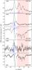 |
Fig. 1 Single-sideband spectra of NH2 towards W31C. The blue arrows mark the relative positions and intensities of the strongest hyperfine structure components (>10% of the main hfs). The dotted line shows the VLSR of the source and the red box the VLSR range for the line-of-sight interstellar gas. |
In summary, our approach to estimating the OPR is to compare the absorption of the lowest ortho and para lines at 953 GHz and 1444 GHz, respectively. We calculate the opacities in each velocity bin, and then convert this opacity ratio into a column density ratio. In this way, we find the OPR in different types of physical conditions traced by the absorption lines: the molecular envelopes surrounding the hot cores, the line-of-sight translucent gas, and one dense and cold core (the filament interacting with W51). For the hot cores themselves it is not possible to reliably estimate the OPR, however, since we only have one para line that mainly traces lower excitation gas in the envelopes.
However, before the above procedure was performed we addressed three problems: (i) The complex hyperfine structure of the different transitions that prevents a direct comparison of the spectra. This was solved by deconvolving the observed lines with respective hfs patterns. (The line blending prevents an independent calculation of the opacities from the observed hyperfine structure components). (ii) Emission from the hot cores that may be present at a low level in the 953 and 1444 GHz lines, although hidden by the strong absorption of the foreground molecular envelope. By assuming that the emission from the hot core is separated from the absorption of the foreground molecular envelope, we used the more highly excited transitions to construct a model of the hot core emission. The modelled emission line profiles of the 953 and 1444 GHz lines were then removed from the observed spectra. (iii) The excitation in the molecular envelopes themselves affects the absorption depths, and the derived opacities will be underestimated. Hence the excitation temperature cannot be neglected in these regions. This is, however, most likely not a major problem in the translucent interstellar gas, where the excitation is most likely low or completely negligible.
Below we describe the details of our analysis and modelling.
3.1. ALI modelling: hot core emission and excitation in the envelopes
To find the underlying emission line structure of the 953 GHz ortho and 1444 GHz para lines in the hot cores and to examine the excitation in the envelopes, we used a non-LTE, one-dimensional, radiative transfer model based on the accelerated lambda iteration (ALI) scheme (Rybicki & Hummer 1991) to solve the radiative transfer in a spherically symmetric model cloud. ALI has been tested and used, for example by Maercker et al. (2008) and Wirström et al. (2014). We also used this code in our current modelling of our Herschel-HIFI observations of seven rotational ammonia transitions in G34.3 (Hajigholi et al. 2016), and W31C, W49N and W51 (Persson et al., in prep.). Collision rates for neutral impact on NH2 were estimated based upon an assumed quenching rate coefficient of 5 × 10-11 cm3 s-1 and state-specific downward rates for radiatively allowed transitions that scale in proportion to radiative line strengths.
For our NH2 observations, we constructed a simple homogeneous spherical clump model for the hot core emission in all sources. This model was fitted to the excited emission lines that show no or very little evidence of self-absorption. In a second model, fitted to all lines seen in both emission and absorption, we added an outer envelope with lower density and temperature in an attempt to also reproduce the major features of the absorption, in order to derive an estimate of the excitation temperature in the outer envelopes. The best fits were found by varying the temperature and density until the modelled 649 GHz line matched the observed one. The relative strengths of the 649 and 907 GHz lines are sensitive to the source size and only weakly dependent on dust temperature; the 649 GHz line becomes weaker with respect to the 907 GHz line with increasing size. We then searched for a combination that produced the best agreement with the continuum levels for all transitions. The large number of hfs components makes the modelling very time-consuming, however. We acknowledge that we therefore have not fully explored the large parameter space, and other solutions that fit our observed data are thus certainly possible. For our purpose, however, other solutions only have a minor impact on the modelled emission line profiles for the 953 GHz line, shown in Figs. A.5−A.8, which were removed from the observed spectra together with the continuum in the normalisation (Sect. 3.4). The modelled emission from the hot cores in the para line is all below the noise levels and was therefore not removed from the observed spectra.
Our attempt to use a simple two-component model to reproduce the full line profiles was successful towards W31C, where our best-fit model to all lines is shown in Fig. 5. In this model, the ortho abundances in the hot core and envelope are 5 × 10⁻¹⁰ and 2 × 10⁻⁹, respectively, and the OPR in the envelope is 2.6. The excitation temperatures for the ortho and para line are 12.8 and 17.4 K, respectively.
The ortho 953 GHz line was much more difficult to model in the remaining sources – a more complex density, temperature, and velocity distributions are most likely required. Examples of (unsuccessful) models of both the emission and absorption towards W49N, W51 and G34.3 are shown in Figs. A.9−A.11. The ALI input parameters for all sources are listed in Table B.7, including the resulting excitation temperatures used in Sect. 3.2 to correct the opacities. Since we did not succeed to model the depth of the ortho absorption, we used the derived excitation temperatures as upper limits.
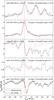 |
Fig. 5 W31C. A two-component ALI model of the hot core emission at VLSR = −3.5 km s-1 (marked with a vertical dashed line), and foreground envelope absorption at VLSR = 0 km s-1. The absorptions from interstellar gas along the sight-lines at VLSR = 11−50 km s-1 are not modelled. The relative difference of the modelled and observed continuum at the frequency of each line is given in the legend. The resulting ortho-to-para ratio for this model is 2.6 in the envelope. |
3.2. Excitation effect on the opacity
The optical depths per unit velocity interval, τν, are derived from  (1)where TMB and TC,MB are the observed antenna and continuum temperature, respectively, corrected for the beam efficiency, and
 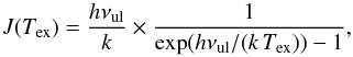 (2)where νul is the frequency of the transition, and Tex the excitation temperature. We here assume that the foreground absorbing material completely fills the beam and covers the continuum. This assumption is supported by the ALI modelling in Sect. 3.1.
Solving Eq. (1) for the opacity, we find 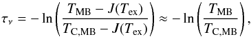 (3)where the last approximation is only valid when Tex ≪ hνul/k = 46 and 69 K for the ortho and para line, respectively. At low temperatures, the main influence of the excitation temperature is on the ortho line, since the quantity J(Tex) is a sensitive function of frequency and the excitation temperature, as shown in Fig. A.4. Taking into account the non-thermalised populations and thus different excitation temperatures for the ortho and para species, we find that when using the excitation temperatures derived with the ALI code (listed in Table B.7), where Tex for ortho is lower than for para, the differences in J(Tex) decrease to ~1−10%. However, the stronger continuum at the frequency of the para line reduces the effect of excitation on this line. Neglecting the excitation gives opacities of 0.6 and 0.27 of the main hyperfine components of the ortho and para lines, respectively, in the molecular envelope of W31C. Including the J(Tex) correction, the opacities in the respective lines increase to 0.9 and 0.31. However, for the other three sources, where the excitation temperature is higher, the effect on the OPR from the para line increases due to the rapid increase of J(Tex).
3.3. From opacities to column densities
Since we were unable to model all sources with ALI, we used the non-equilibrium homogeneous radiative transfer code RADEX5 (van der Tak et al. 2007) to convert opacities into column densities, taking into account both observed and unobserved levels. We used the same collision rates as for the ALI modelling. The principal input parameters are the molecular hydrogen density and kinetic temperature TK. The column density was varied until the integrated opacity was unity. The conversion factors were estimated in the ranges n(H2) = 500−3000 cm-3 and kinetic temperatures TK = 30−100 K for the translucent interstellar gas, and n(H2) = 104−106 cm-3 and TK = 15−70 K for the source molecular envelopes and the dense, cold clump in W51. The results are not very sensitive to changes in density or temperature because of the high critical densities of the NH2 transitions (ncrit = 108−109 cm-3). For the line-of-sight gas, we used the average Galactic background radiation in the solar neighbourhood plus the cosmic microwave background radiation as background radiation field, and for the source molecular clouds we included the respective observed spectral energy distribution. In translucent cloud conditions, the integrated opacity is 1.0 km s-1 for the 953 GHz and 1444 GHz transitions when N(ortho-NH2) = 3.6 × 1012 cm-2, and N(para-NH2) = 8.1 × 1012 cm-2, respectively. The ratio of the conversion factors is 2.25, which corresponds to a factor of 6.8 for an OPR of three. The ratio is similar to within ≲20% for all our investigated physical conditions.
3.4. Ortho-to-para results
The upper panels in Figs. 6–9 show the ortho 953 GHz and para 1444 GHz lines, where the intensities have been normalised to the continuum in a single sideband as  . The middle panels show the spectra after three corrective steps have been applied:
-
Emissions from the central sources were removed by addingmodelled emission profiles to the continuum levels that in turnwere used for the normalisation (emission is treated as a variationin the background continuum).
-
A deconvolution algorithm was applied to provide spectra that only contain the main hfs component. The assumption used is that in the optical depth domain, our spectra can be treated as a set of single-line velocity components that have been convolved with an hfs structure according to the expected LTE relative optical depths (Tables B.2–B.6).
-
We include correction for the excitation by applying our best estimate of Tex in a velocity range around the source velocity, meaning that in these ranges the normalisation is made through (TMB−J(Tex))/(TC,MB−J(Tex)). No corrections were made for the line-of-sight components.
In the lower panels, the left hand y-axis shows the optical depth ratios for the strongest hfs components. The corresponding column density ratios, summed over all hfs components (a correction factor of 4.5/2.25), are given by the right hand y-axis. To convert from opacity ratios into column density ratios, we used the conversion factors obtained with RADEX. We only included data points where the absorption depths of both ortho and para exceeded five times the thermal root mean square (rms), as measured in line-free regions of the baseline. In a few cases we show lower limits, where only the ortho line satisfies this condition. Assuming that the OPR is constant across the line profile in each velocity component, we show the equally weighted averages of ratios over velocity ranges in magenta. All the resulting OPR averages are listed in Table 3.
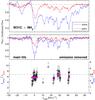 |
Fig. 6 W31C. Upper: normalised spectra of the ortho 953 GHz and para 1444 GHz lines. Middle: deconvolved spectra where the strongest hfs component is plotted for both transitions. The hot core VLSR is marked with a dotted vertical line. Lower: the optical depth and column density ratios of the convolved spectra as functions of VLSR for absorptions larger than 5σ. The horizontal dashed line marks the high-temperature OPR limit of three. (Details are found in Sect. 3.4.) |
In summary, we find a value above the statistical limit in the molecular envelope of W49N, 3.5 ± 0.1 (formal errors), while for the other three molecular envelopes we find values slightly below three, in the range (2.3−2.7) ± 0.1. In the translucent interstellar gas towards W31C we find similar values of (2.2−2.9) ± 0.2. However, we also obtain values above three in the translucent gas; towards W31C we find one component with ≳4.2, and, similarly, towards W49N one component with ≳5.0. In addition, we find an OPR of 3.4 ± 0.1 in the redshifted dense and cold filament interacting with W51 at VLSR ~ 68 km s-1.
3.5. Uncertainties
The 1σ errors shown in Figs. 6–9 and given in Table 3 correspond to quadratically summed uncertainties that are due to thermal noise and and calibration, including uncertainties in the gain ratios of upper and lower sidebands. The variation within the dynamical velocity components seems to be somewhat larger than the formal errors when averaging over components. We do not know at this time if this is a real chemical effect or a symptom of imperfections in our approach or data.
Additional uncertainties, much more difficult to estimate accurately, consist of errors in the deconvolution, emission from the background hot cores, and the excitation. The deconvolution was checked by comparison of the main hfs component of the respective line obtained from the deconvolution with the results from Gaussian fits with good agreements. Examples are shown for W31C in Figs. A.2, A.3, where we have used the results from the Gaussian fitting performed in paper II. The emission of the ortho line from the background hot core has a minor impact on the derived OPR. For example, in W31C we obtain an OPR of 1.6 without any of the emission or correction for excitation. Adding the removal of emission the mean OPR increases to 1.8.
Resulting average OPRs, observed temperatures, TK, and the temperature ranges in which the OPRs are reproduced by model b, Tmod, for a density of nH = 2 × 104 cm-3 (Fig. 10) in the molecular envelopes and the dense core associated with W51, and nH = 1 × 103 cm-3 for the translucent gas (Fig. A.12).
The largest uncertainty in the derived OPR is the excitation, as shown in Fig. A.4. Using Eq. (3), we find upper limits to the excitation temperatures as follows: Tex(ortho) ≲ 15.1 K, ≲17.0 K, ≲17.4 K, and ≲10.5 K, and Tex(para) ≲ 29 K, ≲34 K, ≲33 K, and ≲26 K, in the W31C, W49N, W51, and G34.3 molecular envelopes, respectively. Applying the correction from the ALI modelling in W31C, Tex(ortho) = 12.8 K and Tex(para) = 17.4 K, we find that the mean OPR increases from 1.8 to 2.5. It is clear that if the excitation temperatures are underestimated, the derived OPRs will also be underestimated and could reach, or exceed, the thermal equilibrium value. However, the opposite is also true. The OPRs will be overestimated if we apply too high excitation temperatures. The result in the W31C molecular envelope, OPR = 2.5 ± 0.1, can, however, be compared to the ALI model, where we find a similar value of 2.6 (Fig. 5), in support of an OPR below three. Towards G34.3, we used an ortho excitation temperature that equals the upper limit obtained from the observed almost saturated line, which supports a mean OPR below three in this source as well, even though the para excitation may also play a role. For W49N and W51 the excitation temperature is more difficult to pinpoint, since we were not able to find good ALI models, and the upper limits are rather high. The OPR in these sources may in fact have been overestimated since we have used the Tex derived from the ALI models that did not reproduce the depth of the ortho absorptions, partly because the excitation temperature was too high.
Assuming that the excitation along the sight-line gas is low, the OPR in these components is not affected and hence can be considered as more robust than the results in the molecular envelopes. However, Emprechtinger et al. (2013) showed that the assumption that all population of water is in the ground state is not valid in the foreground gas towards NGC 6334I. The ortho-NH2 953 GHz line is less affected by the excitation than the ortho-H2O 557 GHz line, however. Flagey et al. (2013) studied the water OPR along the same sight-lines as analysed in this paper and found from analysing the two ortho ground-state transitions at 557 GHz and 1 669 GHz that Tex ≈ 5 K. Assuming that NH2 and NH3 co-exist, we checked in addition our ammonia data along the same sight-lines as reported in this paper. We observed ammonia JK = 10–00, 20–10, 30–20, 21–11, 31–21, and 32–22 lines and find no signs of absorptions, except for the lines connecting to the lowest ground states. This suggests that the excitation is also negligible in the 953 GHz and 1444 GHz NH2 lines (see Hajigholi et al. 2016, for ALI modelling of ammonia in G34.3).
4. Chemistry and ortho-to-para relation of NH2
In this section we apply a gas-phase chemistry model that takes the nuclear-spin symmetries of molecular hydrogen and the nitrogen hydrides into account. The model was developed for cold and dense gas conditions, however, which are representative of our molecular envelopes, and it therefore cannot fully exploit the chemistry in the translucent line-of-sight gas. Work is in progress to include photodissociation and photoionisation reactions and the effect of variation in AV, as well as surface chemistry.
4.1. OPR in equilibrium
The OPR can be expressed as the ratio of the sum of the populations of the energy levels of ortho-NH2 to those of para-NH2. If interconversion between ortho and para states is possible and efficient, at local thermodynamical equilibrium (LTE), the populations of the energy levels follow a Boltzmann distribution. The OPR is then computed by the ratio of partition functions of the ortho and para forms as 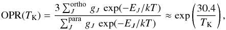 (4)where EJ stands for the energy of the rotational levels (even though rotation is handled by the three quantum numbers J, Ka, Kc in an asymmetric top). The fine-structure and hyperfine-structure contributions to the energy are omitted for simplicity. The rotational degeneracy is denoted by gJ. The approximation is valid for low temperatures (T ≲ 20 K), where only the ground states are populated and the partition functions are reduced to the degeneracies of the lowest rotational state in each form, which are equal (ignoring the fine and hyperfine structure splitting). The energy difference between the two ground spin states is 30.4 K (see Fig. A.1). As illustrated in Fig. 10, the OPR in thermal equilibrium increases with decreasing temperature.
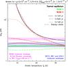 |
Fig. 10 OPR of NH2 computed as a function of kinetic temperature for a density of nH = 2 × 104 cm-3: (i) at thermal equilibrium (black solid line); (ii) with model a (green, Sect. 4.2); and (iii) with model b (red, corresponding to model a plus the NH2 + H reaction, Sect. 4.3). The OPR is plotted at four different times for both models: 1 × 10⁴ yr (solid lines), 5 × 10⁵ yr (dashed lines), 106 yr (dotted lines), and steady-state (dashed-dotted lines). The hatched boxes represent our best estimates of the average OPR, including formal error bars. In blue we show the W31C, W51, and G34.3 molecular envelopes, and in pink the filament connected to W51 at VLSR ~ 68 km s-1 and the W49N molecular envelope. |
4.2. Deviation from thermodynamical equilibrium
The pink hatched box in Fig. 10 shows the range of observed OPR values, including their formal errors, in the molecular envelope of W49N and the cold and dense filament connected to W51 at VLSR ~ 68 km s-1. Both OPR values lie above three, while the blue hatched box shows the range of observed OPR values in the molecular envelopes of W31C, W51, and G34.3. These values lie below three. Measurements of an OPR lower than its thermal equilibrium value in the molecular envelopes can be due to the non-LTE OPR of H2 pertaining at the low temperatures of these environments. Studies of the OPR of H2 in dense and cold gas (Le Bourlot 1991, 2000; Takahashi 2001; Flower et al. 2006; Pagani et al. 2009) have indeed shown that at low temperatures (<20 K) the OPR is controlled by kinetic and not by thermodynamical considerations. At 10 K, model estimates predict an OPR of about 10-3 (Le Bourlot 1991; Flower et al. 2006), far higher than the equilibrium value of 3 × 10⁻⁷. Moreover, recent observations of multi-hydrogenated species such as NH3 (Persson et al. 2012) and H (Crabtree et al. 2011) show values that significantly depart from thermal equilibrium. Several measurements of the water OPR have been made, and most indicate values close to the LTE value of three (Emprechtinger et al. 2013; Flagey et al. 2013), although exceptions have been observed. Lis et al. (2013) found an average OPR along the sight-line towards Sgr B2 (N) of 2.34 ± 0.25, indicating a spin temperature of 24-32 K in thermal equilibrium. Flagey et al. (2013) found values of 2.3 ± 0.1 and 2.4 ± 0.2 in the +40 and +60 km s-1 components towards W49N, respectively, indicating a spin temperature of ~25 K. Other species show OPRs consistent with LTE values, for example H2O+ (Schilke et al. 2013; Gerin et al. 2013) and H2Cl+ (Gerin et al. 2013; Neufeld et al. 2015) within the error bars.
The OPR of H2 has a major impact on the key reaction initiating the nitrogen hydride synthesis in cold gas conditions, N+ + H2 → NH+ + H, which possesses a small endoergicity of the order of the energy difference between the lowest rotational fundamental states of ortho- and para-H2 (~170 K, Gerlich 2008). A succession of hydrogenations of the NH ions (with n = 1−3) follows, leading to the formation of the ion ammonium (NH
 ). Once formed, NH undergoes dissociative recombination with electrons resulting in the production of NH3 and NH2 (see Fig. 3 in Persson et al. 2014). NH2 can also form through the dissociative recombination of NH. This pathway, which is not the dominant one for dense and cold gas, will be more efficient for diffuse and translucent gas, where the electron fraction can be relatively higher, and hence the OPR of NH2 will directly depend on the OPR of NH in these environments. However, since NH
 is itself formed through NH + H2, directly or indirectly, the OPR of NH2 will always depend on that of NH.
Considering that the electron recombination rates are equal for the different nuclear spin species, it is thus the proportion of each form of NH (para (I = 0), ortho (I = 1), and meta (I = 2)), and also to a lesser extent each form of NH (depending on the properties of the gas considered), that will impact the OPR of NH2. In the cold interstellar medium, the gas-phase production of NH2 therefore mainly proceeds from NH, while it is destroyed by atomic carbon and oxygen. Since the destruction rates for the ortho and para forms are considered to be equal, the OPR of NH2 is mainly determined by the nuclear spin branching ratios in the electron recombinations of the three spin configuration of NH (Rist et al. 2013; Le Gal et al. 2014) viz.,
  (5)Photodissociation of NH3 in diffuse and translucent gas can also form NH2, but this pathway is not expected to have a major impact on our results. The selection rules should, moreover, be the same as those for the reaction NH + e−. Thus, even if the photodissociation of NH3 pathway is the dominant one in the formation of NH2 in diffuse and translucent gas, the effect of the photodissociation of NH3 will be to enhance the NH + e− reaction formation pathway outcome in the production of the OPR of NH2.
To reproduce the observed OPRs presented in this paper, we used the astrochemical model developed in Le Gal et al. (2014), which is based on gas-phase nuclear-spin conservation chemistry of the nitrogen hydrides, considering nuclear-spin conservation and full scrambling selection rules for the multi-hydrogenated nitrogen molecules. This model6 (hereafter model a) can reproduce the observed OPRs below three in the molecular envelopes of the sources W31C, W51, and G34.3, mostly independently of temperature for 5 <TK< 35 K, for times between ~104 yr and ~106 yr, at a density of nH = 2 × 104 cm-3 and a cosmic-ray ionisation rate of 1.3 × 10⁻¹⁷ s-1. These results are represented in green in Fig. 10. In Fig. A.12 we show a model with a lower density, nH = 1 × 103 cm-3, and a cosmic-ray ionisation rate of 2 × 10-16 s-1, which is compared to our results in the translucent gas.
Model a cannot reproduce the OPR above three found in the filament associated with W51 at VLSR ~ 68 km s-1, however, or the limits ≳4.2 and ≳5.0 along two of the line-of-sight components and in the W49N molecular envelope.
4.3. Possible interconversion between o-NH2 and p-NH2
The ortho and para forms of NH2 can undergo a number of exchange collisions with other hydrogenated species such as atomic hydrogen, allowing interconversion between ortho- and para-NH2. Such processes will increase the OPR with decreasing temperature and lead to LTE for the OPR at steady-state. To explain the OPR values above three, the two following reactions were added to the Le Gal et al. (2014) model: 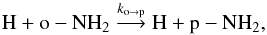 (6)
(6)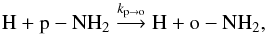 (7)with ko → p = kp → oexp(−30.4 /T). Since these radical-radical rate coefficients have not yet been measured or calculated, we chose for kp → o a typical rate coefficient of 10-10 cm-3 s-1. Whether or not the H-transfer reactions between H and NH2 proceed at a near collisional value is currently uncertain. Experimental evidence from the saturated three-body reaction to produce ammonia indicates at most a small barrier (Pagsberg et al. 1979), while theoretical calculations indicate a more substantial barrier and a conical intersection (McCarthy et al. 1987; Ma et al. 2012). New calculations and experiments are clearly needed.
Results from adding reactions (6) and (7) to our spin chemistry model, without changing any other parameters (hereafter model b), are represented by the red curves in Figs. 10 and A.12. Since model b produces OPRs below the equilibrium value of three for higher temperatures but approaches the LTE ratio with time for low temperatures, it can reproduce all observed OPRs, both below and above three. At early times, ~104 yr, the NH2-OPR in model b does not have time to thermalise and will therefore be close to model a. As shown in Fig. 10, the OPR towards the W49N molecular envelope and the filament connected to W51 (VLSR = + 68 km s-1) is reproduced within a temperature range of 5−13 K at a time equal to ~5 × 10⁵ yr. At later times, the OPR increases more quickly as the temperature decreases, reducing the range of agreement and driving it to higher temperatures. From 106 yr, the range remains constant at 23−25 K. The same model parameters can reproduce the OPR range of (2.3−2.7) ± 0.1 in the envelopes of W31C, W51, and G34.3 within a temperature range of 23−35 K at a time of ~5 × 10⁵ yr as long as the excited rotational levels of ortho and para NH2 have a negligible population. Finally, the lower limits derived in the translucent gas along the sight-lines towards W31C (≳4.2) and W49N (≳5) can be reproduced for temperatures of 17−21 K, and 14−19 K, respectively, depending on time, using nH = 1 × 103 cm-3 as shown in Fig. A.12.
The resulting temperatures at different times that can reproduce the observed OPRs are consistent with the observed temperatures in the different components (modelled and observed temperatures are listed in Table 3), except for the +17 km s-1 component towards W31C and the molecular envelope in W49N. The result in the latter component may suggest that we may have overestimated the OPR in W49N by using a too high excitation temperature. By using Tex(ortho) = 12 K instead of 14 K, for instance, the mean OPR decreases to 3.0.
We note that the resulting timescales are only indicative since our time-dependent models depend on many uncertain physical and chemical parameters. For model b, which reproduces the observed OPRs best, decreasing the density will lower the temperature ranges that reproduce the OPRs for specific timescales at which the thermal equilibrium is not yet reached. The initial chemical conditions can also play an important role in the chemistry. For a given density, increasing the ionisation rate will moreover have the effect of shortening the timescale so that steady-state will be reached faster. In addition, for a given time, the model will require higher temperatures to reproduce the observed OPRs.
If the exchange collisions between H and NH2 are sufficiently reduced in rate, the OPR should lie in between the initial OPR value, when it forms through exothermic dissociative electronic recombinations of NH, and the thermalised value depending upon time (cf. Neufeld et al. 2015). For the model including H-exchange reactions between H and NH2 model b in Figs. 10 and A.12), the ko → p rate coefficient used assumes that only the ground para and ortho states are populated (000 and 101 states). However, the first excited ortho (111) and para (110) levels lie only 45 K and 22 K above their respective ground levels, which implies that the two-level conversion rate is not accurate above ~20 K if the excited rotational states of ortho and para are significantly populated. As suggested in Herbst (2015), two points have to be examined. First, if the density is below the critical density, spontaneous emission dominates collisional effects. In that case, as can occur in diffuse gas where the rotational temperature can be quite low, the OPR is approximated by Eq. (4). Secondly, if chemical equilibrium is not reached, the OPR should be kinetically controlled (as in Eq. (5)). Once formed, the para and ortho NH2 relax towards lower rotational states for each nuclear spin state preserving the original OPR. If the relaxation occurs mainly by spontaneous emission, the lowest rotational states will be formed predominantly. Afterwards, a competition ensues between spin equilibration, which in model b mostly occurs via exchange collisions with H atoms, and destruction processes with a variety of radicals. If destruction dominates, the eventual OPR will be kinetically controlled.
As a comparison with the OPR observations of NH3 already published in Persson et al. (2012) and also to highlight the coherence of our ortho-para model, we present the results of models a and b for the OPR values of NH3 in Fig. A.13, where we have used the same physical parameters as for the lower density NH2-OPR model. The hatched box marks the observed NH3-OPR values along the sight-lines towards W31C and W49N (Persson et al. 2012). Our model can reproduce the observed OPRs depending on the physical conditions and timescales considered. Increasing the cosmic-ray ionisation rate or decreasing the density decreases the steady-state value of the NH3 OPR, which shortens the modelled timescales necessary to reproduce the observed OPR values.
Most of the NH2-OPR values derived from the observations presented in this paper are consistent with a gas-phase spin nitrogen chemistry including H-exchange reactions between H and NH2. We therefore did not include surface chemistry in our model, except for the formation of H2 and charge exchanges. Future development of our model will include the possibility of ortho-para conversion on cold grain surfaces, which may take place in molecular clouds with low temperature and high density where gas-phase species condense on the surface of grains (Tafalla et al. 2002). The efficiency of this phenomenon depends on the time the species reside on the grain, on the grain surface shape, and on the time of nuclear spin conversion. However, the characteristic nuclear-spin conversion times on grain surfaces are not yet well constrained (Le Bourlot 2000; Chehrouri et al. 2011; Hama & Watanabe 2013). Neither did we consider forbidden spontaneous emission (Tanaka et al. 2013) or state-specific formation and destruction in our models, which might also help to explain the OPR values above three. In diffuse gas, the UV radiation might also play a significant role in the nitrogen chemistry by photo-dissociation (Persson et al. 2012), although we do not expect that UV radiation significantly changes the OPR of nitrogen hydrides, which is mainly driven by proton transfer reactions.
5. Conclusions
We have derived ortho-to-para ratios of NH2 both above and below the statistical value of three. In the molecular envelopes surrounding three of our observed hot cores, we found average OPRs below three and similar values in the translucent interstellar gas. In contrast, we found an average OPR above three in the dense and cold filament interacting with W51, in addition to two velocity components along the sight-lines towards W31C and W49N and in the molecular envelope in W49N. The results in the line-of-sight interstellar gas are considered to be more robust than in the source molecular clouds because of the lower or completely negligible excitation. Using a non-LTE radiative transfer model based on the accelerated lambda iteration scheme, we successfully modelled the emission and absorption in the W31C molecular envelope supporting an OPR below three. The derived OPR below three in the G34.3 molecular envelope is also considered as more robust than the results in the W49N and W51 molecular envelopes, since we used the upper limit of the ortho excitation temperature when correcting the opacities for excitation.
Astrochemical models considering nuclear-spin gas-phase chemistry in a “para-enriched H2” gas can reproduce the variations of the observed ortho-to-para ratios of NH2 and NH3 below their statistical value of three and unity, respectively. The NH2 OPR values higher than three can be explained by including in these models the thermalisation reaction NH2 + H with efficient ortho-to-para and para-to-ortho rate coefficients and selected intervals of time.
Developed by Per Bergman at Onsala Space Observatory, Sweden; http://www.chalmers.se/rss/oso-en/observations/data-reduction-software
The model derived from Le Gal et al. (2014) used in this paper has been corrected for a typo in branching ratios for the NH + H2 reaction. This implies that the observed OPRs in the range 2.2 to 2.8, discussed in this paper, are no longer reproduced at steady-state, but at earlier times (see Fig. 10).
Acknowledgments
HIFI has been designed and built by a consortium of institutes and university departments from across Europe, Canada and the United States under the leadership of SRON Netherlands Institute for Space Research, Groningen, The Netherlands and with major contributions from Germany, France and the US. Consortium members are: Canada: CSA, U.Waterloo; France: CESR, LAB, LERMA, IRAM; Germany: KOSMA, MPIfR, MPS; Ireland, NUI Maynooth; Italy: ASI, IFSI-INAF, Osservatorio Astrofisico di Arcetri- INAF; Netherlands: SRON, TUD; Poland: CAMK, CBK; Spain: Observatorio Astronómico Nacional (IGN), Centro de Astrobiología (CSIC-INTA). Sweden: Chalmers University of Technology – MC2, RSS & GARD; Onsala Space Observatory; Swedish National Space Board, Stockholm University – Stockholm Observatory; Switzerland: ETH Zurich, FHNW; USA: Caltech, JPL, NHSC. Support for this work was provided by NASA through an award issued by JPL/Caltech. C.P., E.S. and M.O. acknowledge generous support from the Swedish National Space Board. R. L. and E. H. acknowledge support for this work provided by NASA through an award issued by JPL/Caltech. A.F. acknowledges support from the Agence Nationale de la Recherche (ANR-HYDRIDES), contract ANR-12-BS05-0011-01. M.G. and D.L. acknowledge support from Centre Nationale d’Etudes Spatiales (CNES) and the CNRS/INSU programme de physique et chimie du milieu interstellaire (PCMI).
References
- Cernicharo, J., Goicoechea, J. R., & Caux, E. 2000, ApJ, 534, L199 [NASA ADS] [CrossRef] [PubMed] [Google Scholar]
- Chehrouri, M., Fillion, J.-H., Chaabouni, H., et al. 2011, Phys. Chem. Chem. Phys. (Incorporating Faraday Transactions), 13, 2172 [NASA ADS] [CrossRef] [Google Scholar]
- Crabtree, K. N., Indriolo, N., Kreckel, H., Tom, B. A., & McCall, B. J. 2011, ApJ, 729, 15 [NASA ADS] [CrossRef] [Google Scholar]
- de Graauw, T., Helmich, F. P., Phillips, T. G., et al. 2010, A&A, 518, L4 [EDP Sciences] [Google Scholar]
- De Luca, M., Gupta, H., Neufeld, D., et al. 2012, ApJ, 751, L37 [NASA ADS] [CrossRef] [Google Scholar]
- Emprechtinger, M., Lis, D. C., Rolffs, R., et al. 2013, ApJ, 765, 61 [NASA ADS] [CrossRef] [Google Scholar]
- Faure, A., Hily-Blant, P., Le Gal, R., Rist, C., & Pineau des Forêts, G. 2013, ApJ, 770, L2 [NASA ADS] [CrossRef] [Google Scholar]
- Fazio, G. G., Lada, C. J., Kleinmann, D. E., et al. 1978, ApJ, 221, L77 [NASA ADS] [CrossRef] [Google Scholar]
- Flagey, N., Goldsmith, P. F., Lis, D. C., et al. 2013, ApJ, 762, 11 [NASA ADS] [CrossRef] [Google Scholar]
- Flower, D. R., Pineau Des Forêts, G., & Walmsley, C. M. 2006, A&A, 449, 621 [NASA ADS] [CrossRef] [EDP Sciences] [Google Scholar]
- Gerin, M., de Luca, M., Goicoechea, J. R., et al. 2010, A&A, 521, L16 [Google Scholar]
- Gerin, M., de Luca, M., Lis, D. C., et al. 2013, J. Phys. Chem. A, 117, 10018 [CrossRef] [Google Scholar]
- Gerin, M., Ruaud, M., Goicoechea, J. R., et al. 2015, A&A, 573, A30 [NASA ADS] [CrossRef] [EDP Sciences] [Google Scholar]
- Gerlich, D. 2008, in Low Temperatures and Cold Molecules (London: Imperial College Press), 121 [Google Scholar]
- Goicoechea, J. R., Rodríguez-Fernández, N. J., & Cernicharo, J. 2004, ApJ, 600, 214 [NASA ADS] [CrossRef] [Google Scholar]
- Hajigholi, M., Persson, C. M., Wirström, E. S., et al. 2016, A&A, 585, A158 [NASA ADS] [CrossRef] [EDP Sciences] [Google Scholar]
- Hama, T., & Watanabe, N. 2013, Chem. Rev., 113, 8783 [CrossRef] [Google Scholar]
- Herbst, E. 2015, in Web Conf., 84, 6002 [Google Scholar]
- Kurayama, T., Nakagawa, A., Sawada-Satoh, S., et al. 2011, PASJ, 63, 513 [NASA ADS] [Google Scholar]
- Le Bourlot, J. 1991, A&A, 242, 235 [NASA ADS] [Google Scholar]
- Le Bourlot, J. 2000, A&A, 360, 656 [Google Scholar]
- Le Gal, R., Hily-Blant, P., Faure, A., et al. 2014, A&A, 562, A83 [NASA ADS] [CrossRef] [EDP Sciences] [Google Scholar]
- Lis, D. C., Bergin, E. A., Schilke, P., & van Dishoeck, E. F. 2013, J. Phys. Chem. A, 117, 9661 [CrossRef] [Google Scholar]
- Ma, J., Zhu, X., Guo, H., & Yarkony, D. R. 2012, J. Chem. Phys., 137, 22A541 [Google Scholar]
- Maercker, M., Schöier, F. L., Olofsson, H., Bergman, P., & Ramstedt, S. 2008, A&A, 479, 779 [NASA ADS] [CrossRef] [EDP Sciences] [Google Scholar]
- McCarthy, M. I., Rosmus, P., Werner, H.-J., Botschwina, P., & Vaida, V. 1987, J. Chem. Phys., 86, 6693 [NASA ADS] [CrossRef] [Google Scholar]
- Mookerjea, B., Vastel, C., Hassel, G. E., et al. 2014, A&A, 566, A61 [NASA ADS] [CrossRef] [EDP Sciences] [Google Scholar]
- Müller, H. S. P., Klein, H., Belov, S. P., et al. 1999, J. Mol. Spectr., 195, 177 [NASA ADS] [CrossRef] [Google Scholar]
- Müller, H. S. P., Thorwirth, S., Roth, D. A., & Winnewisser, G. 2001, A&A, 370, L49 [NASA ADS] [CrossRef] [EDP Sciences] [Google Scholar]
- Müller, H. S. P., Schlöder, F., Stutzki, J., & Winnewisser, G. 2005,J. Mol. Struct., 742, 215 [Google Scholar]
- Mueller, K. E., Shirley, Y. L., Evans, II, N. J., & Jacobson, H. R. 2002, ApJS, 143, 469 [NASA ADS] [CrossRef] [Google Scholar]
- Neufeld, D. A., Black, J. H., Gerin, M., et al. 2015, ApJ, 807, 54 [NASA ADS] [CrossRef] [Google Scholar]
- Ott, S. 2010, in ASP Astronomical Data Analysis Software and Systems XIX, eds. Y. Mizumoto, K.-I. Morita, & M. Ohishi, Conf. Ser., 434, 139 [Google Scholar]
- Pagani, L., Daniel, F., & Dubernet, M.-L. 2009, A&A, 494, 719 [NASA ADS] [CrossRef] [EDP Sciences] [Google Scholar]
- Pagsberg, P. B., Eriksen, J., & Christensen, H. C. 1979, J. Phys. Chem., 83, 582 [CrossRef] [Google Scholar]
- Persson, C. M., Black, J. H., Cernicharo, J., et al. 2010, A&A, 521, L45 (Paper I) [NASA ADS] [CrossRef] [EDP Sciences] [Google Scholar]
- Persson, C. M., De Luca, M., Mookerjea, B., et al. 2012, A&A, 543, A145 (Paper II) [NASA ADS] [CrossRef] [EDP Sciences] [Google Scholar]
- Persson, C. M., Hajigholi, M., Hassel, G. E., et al. 2014, A&A, 567, A130 [NASA ADS] [CrossRef] [EDP Sciences] [Google Scholar]
- Pilbratt, G., Riedinger, J. R., Passvogel, T., et al. 2010, A&A, 518, L1 [CrossRef] [EDP Sciences] [Google Scholar]
- Polehampton, E. T., Baluteau, J., Swinyard, B. M., et al. 2007, MNRAS, 377, 1122 [NASA ADS] [CrossRef] [Google Scholar]
- Rist, C., Faure, A., Hily-Blant, P., & Le Gal, R. 2013, J. Phys. Chem. A, 117, 9800 [Google Scholar]
- Roelfsema, P. R., Helmich, F. P., Teyssier, D., et al. 2012, A&A, 537, A17 [NASA ADS] [CrossRef] [EDP Sciences] [Google Scholar]
- Rybicki, G. B., & Hummer, D. G. 1991, A&A, 245, 171 [NASA ADS] [Google Scholar]
- Sanna, A., Reid, M. J., Menten, K. M., et al. 2014, ApJ, 781, 108 [NASA ADS] [CrossRef] [Google Scholar]
- Sato, M., Reid, M. J., Brunthaler, A., & Menten, K. M. 2010,ApJ, 720, 1055 [Google Scholar]
- Schilke, P., Lis, D. C., Bergin, E. A., Higgins, R., & Comito, C. 2013, J. Phys. Chem. A, 117, 9766 [CrossRef] [PubMed] [Google Scholar]
- Sonnentrucker, P., Neufeld, D. A., Phillips, T. G., et al. 2010, A&A, 521, L12 [NASA ADS] [CrossRef] [EDP Sciences] [Google Scholar]
- Tafalla, M., Myers, P. C., Caselli, P., Walmsley, C. M., & Comito, C. 2002, ApJ, 569, 815 [NASA ADS] [CrossRef] [Google Scholar]
- Takahashi, J. 2001, ApJ, 561, 254 [NASA ADS] [CrossRef] [Google Scholar]
- Tanaka, K., Harada, K., & Oka, T. 2013, J. Phys. Chem. A, 117, 9584 [CrossRef] [Google Scholar]
- van der Tak, F. F. S., Black, J. H., Schöier, F. L., Jansen, D. J., & van Dishoeck, E. F. 2007, A&A, 468, 627 [NASA ADS] [CrossRef] [EDP Sciences] [Google Scholar]
- van der Tak, F. F. S., Chavarría, L., Herpin, F., et al. 2013, A&A, 554, A83 [NASA ADS] [CrossRef] [EDP Sciences] [Google Scholar]
- van Dishoeck, E. F., Jansen, D. J., Schilke, P., & Phillips, T. G. 1993, ApJ, 416, L83 [NASA ADS] [CrossRef] [Google Scholar]
- Vastel, C., Spaans, M., Ceccarelli, C., Tielens, A. G. G. M., & Caux, E. 2001, A&A, 376, 1064 [NASA ADS] [CrossRef] [EDP Sciences] [Google Scholar]
- Wirström, E. S., Charnley, S. B., Persson, C. M., et al. 2014, ApJ, 788, L32 [NASA ADS] [CrossRef] [Google Scholar]
- Zhang, B., Reid, M. J., Menten, K. M., et al. 2013, ApJ, 775, 79 [NASA ADS] [CrossRef] [Google Scholar]
Appendix A: Additional figures
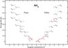 |
Fig. A.1 Energy level diagram of NH2. The observed transitions in this paper are marked in red. |
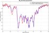 |
Fig. A.2 W31C. Red: original observations (channel separation 0.157 km s-1) with subtracted emission. Blue: Gaussian fits of all velocity (and hfs) components. Line widths and vLSR for each velocity component were taken from the results of the simultaneous Gaussian fitting of NH, ortho-NH2, and ortho-NH3 (method I, described in paper II). |
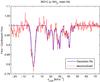 |
Fig. A.3 W31C. Red: the strongest hfs component of para-NH2 obtained from deconvolution. Blue: the strongest hfs component of para-NH2 obtained from Gaussian fits of the opacities. Line widths and vLSR for each velocity component were taken from the results of the simultaneous Gaussian fitting of NH, ortho-NH2, and ortho-NH3 (method I, described in Paper II). |
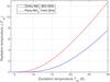 |
Fig. A.4 Radiation temperature J(Tex) as a function of the excitation temperature Tex of the ortho 11,13/2−00,01/2 (953 GHz) and para 21,25/2−10,13/2 (1444 GHz) lines. |
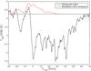 |
Fig. A.5 W31C. Modelled ortho emission from the hot core with the ALI code (parameters are listed in Table B.7). |
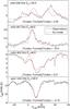 |
Fig. A.9 Example of a simple ALI model of the W49N hot core and the surrounding envelope (parameters are listed in Table B.7). The relative difference of the modelled and observed continuum at the frequency of each line is given in the respective legend. The 649 GHz line suffers from contamination from the image sideband and is used as an upper limit of its true intensity. |
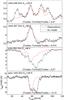 |
Fig. A.10 W51. Notation as in Fig. A.9. The foreground absorption centred at VLSR = 68 km s-1 is not modelled. |
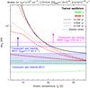 |
Fig. A.12 Calculated OPR of NH2 shown as a function of kinetic temperature for a density of nH = 1 × 103 cm-3: (i) at thermal equilibrium (black solid line), (ii) with model a (green, Sect. 4.2); and (iii) with model b (red, corresponding to model a plus the NH2 + H reaction, Sect. 4.3). The OPR is plotted for four different times for both models: 1 × 10⁴ yr (solid lines), 5 × 10⁴ yr (dashed lines), 105 yr (dotted lines), and steady-state (dashed-dotted lines). The hatched box represents our best estimates of the average OPR, including formal errors, for the translucent gas towards W31C at VLSR ~ 22,28 and 40 km s-1. The dotted horizontal lines with arrows mark the lower limits in the translucent gas towards W31C at VLSR ~ 17 km s-1 (blue) and W49N at VLSR ~ 39 km s-1 (pink). |
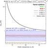 |
Fig. A.13 OPR of NH3 shown as a function of kinetic temperature for a density of nH = 1 × 103 cm-3: (i) at thermal equilibrium (black solid line); (ii) with model a (green) (details in Sect. 4.2); and (iii) with model b (red) (corresponding to model a plus the NH2 + H reaction, details in Sect. 4.3). The OPR is shown at four different times for both models: 1 × 10⁴ yr (solid lines), 5 × 10⁴ yr (dashed lines), 105 yr (dotted lines), and steady-state (dashed-dotted lines). The hatched box represents the OPR of NH3, including formal errors, in the translucent gas in the sight-lines towards W31C and W49N from (Persson et al. 2012). |
Appendix B: Additional tables
Herschel OBSIDs of the observed transitions.
Hyperfine structure components of o-NH2NKa,KcJ = 21,13/2−20,2 3/2.
Hyperfine structure components of o-NH2NKa,KcJ = 20,25/2−11,1 3/2.
Hyperfine structure components of o-NH2NKa,KcJ=11,1 3/2 – 00,0 1/2.
Hyperfine structure components of o-NH2NKa,KcJ = 42,2 9/2−41,3 9/2.
Hyperfine structure components of p-NH2NKa,KcJ = 21,2 5/2-10,1 3/2.
ALI model properties and resulting excitation temperatures.
All Tables
Observed NH2 transitions towards W31C, W49N, W51, and G34.3+0.1, resulting continuum intensities, and noise levels.
Resulting average OPRs, observed temperatures, TK, and the temperature ranges in which the OPRs are reproduced by model b, Tmod, for a density of nH = 2 × 104 cm-3 (Fig. 10) in the molecular envelopes and the dense core associated with W51, and nH = 1 × 103 cm-3 for the translucent gas (Fig. A.12).
All Figures
|
Fig. 1 Single-sideband spectra of NH2 towards W31C. The blue arrows mark the relative positions and intensities of the strongest hyperfine structure components (>10% of the main hfs). The dotted line shows the VLSR of the source and the red box the VLSR range for the line-of-sight interstellar gas. |
| In the text | |
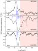 |
Fig. 2 W49N. Notation as in Fig. 1. |
| In the text | |
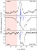 |
Fig. 3 W51. Notation as in Fig. 1. |
| In the text | |
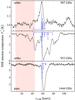 |
Fig. 4 G34.3+0.1. Notation as in Fig. 1. |
| In the text | |
|
Fig. 5 W31C. A two-component ALI model of the hot core emission at VLSR = −3.5 km s-1 (marked with a vertical dashed line), and foreground envelope absorption at VLSR = 0 km s-1. The absorptions from interstellar gas along the sight-lines at VLSR = 11−50 km s-1 are not modelled. The relative difference of the modelled and observed continuum at the frequency of each line is given in the legend. The resulting ortho-to-para ratio for this model is 2.6 in the envelope. |
| In the text | |
|
Fig. 6 W31C. Upper: normalised spectra of the ortho 953 GHz and para 1444 GHz lines. Middle: deconvolved spectra where the strongest hfs component is plotted for both transitions. The hot core VLSR is marked with a dotted vertical line. Lower: the optical depth and column density ratios of the convolved spectra as functions of VLSR for absorptions larger than 5σ. The horizontal dashed line marks the high-temperature OPR limit of three. (Details are found in Sect. 3.4.) |
| In the text | |
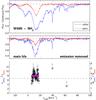 |
Fig. 7 W49N. Notation as in Fig. 6. |
| In the text | |
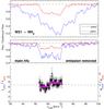 |
Fig. 8 W51. Notation as in Fig. 6. |
| In the text | |
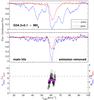 |
Fig. 9 G34.3+0.1. Notation as in Fig. 6. |
| In the text | |
|
Fig. 10 OPR of NH2 computed as a function of kinetic temperature for a density of nH = 2 × 104 cm-3: (i) at thermal equilibrium (black solid line); (ii) with model a (green, Sect. 4.2); and (iii) with model b (red, corresponding to model a plus the NH2 + H reaction, Sect. 4.3). The OPR is plotted at four different times for both models: 1 × 10⁴ yr (solid lines), 5 × 10⁵ yr (dashed lines), 106 yr (dotted lines), and steady-state (dashed-dotted lines). The hatched boxes represent our best estimates of the average OPR, including formal error bars. In blue we show the W31C, W51, and G34.3 molecular envelopes, and in pink the filament connected to W51 at VLSR ~ 68 km s-1 and the W49N molecular envelope. |
| In the text | |
|
Fig. A.1 Energy level diagram of NH2. The observed transitions in this paper are marked in red. |
| In the text | |
|
Fig. A.2 W31C. Red: original observations (channel separation 0.157 km s-1) with subtracted emission. Blue: Gaussian fits of all velocity (and hfs) components. Line widths and vLSR for each velocity component were taken from the results of the simultaneous Gaussian fitting of NH, ortho-NH2, and ortho-NH3 (method I, described in paper II). |
| In the text | |
|
Fig. A.3 W31C. Red: the strongest hfs component of para-NH2 obtained from deconvolution. Blue: the strongest hfs component of para-NH2 obtained from Gaussian fits of the opacities. Line widths and vLSR for each velocity component were taken from the results of the simultaneous Gaussian fitting of NH, ortho-NH2, and ortho-NH3 (method I, described in Paper II). |
| In the text | |
|
Fig. A.4 Radiation temperature J(Tex) as a function of the excitation temperature Tex of the ortho 11,13/2−00,01/2 (953 GHz) and para 21,25/2−10,13/2 (1444 GHz) lines. |
| In the text | |
|
Fig. A.5 W31C. Modelled ortho emission from the hot core with the ALI code (parameters are listed in Table B.7). |
| In the text | |
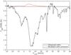 |
Fig. A.6 W49N. Notation as in Fig. A.5. |
| In the text | |
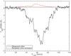 |
Fig. A.7 W51. Notation as in Fig. A.5. |
| In the text | |
 |
Fig. A.8 G34.3. Notation as in Fig. A.5. |
| In the text | |
|
Fig. A.9 Example of a simple ALI model of the W49N hot core and the surrounding envelope (parameters are listed in Table B.7). The relative difference of the modelled and observed continuum at the frequency of each line is given in the respective legend. The 649 GHz line suffers from contamination from the image sideband and is used as an upper limit of its true intensity. |
| In the text | |
|
Fig. A.10 W51. Notation as in Fig. A.9. The foreground absorption centred at VLSR = 68 km s-1 is not modelled. |
| In the text | |
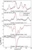 |
Fig. A.11 G34.3+0.1. Notation as in Fig. A.9. |
| In the text | |
|
Fig. A.12 Calculated OPR of NH2 shown as a function of kinetic temperature for a density of nH = 1 × 103 cm-3: (i) at thermal equilibrium (black solid line), (ii) with model a (green, Sect. 4.2); and (iii) with model b (red, corresponding to model a plus the NH2 + H reaction, Sect. 4.3). The OPR is plotted for four different times for both models: 1 × 10⁴ yr (solid lines), 5 × 10⁴ yr (dashed lines), 105 yr (dotted lines), and steady-state (dashed-dotted lines). The hatched box represents our best estimates of the average OPR, including formal errors, for the translucent gas towards W31C at VLSR ~ 22,28 and 40 km s-1. The dotted horizontal lines with arrows mark the lower limits in the translucent gas towards W31C at VLSR ~ 17 km s-1 (blue) and W49N at VLSR ~ 39 km s-1 (pink). |
| In the text | |
|
Fig. A.13 OPR of NH3 shown as a function of kinetic temperature for a density of nH = 1 × 103 cm-3: (i) at thermal equilibrium (black solid line); (ii) with model a (green) (details in Sect. 4.2); and (iii) with model b (red) (corresponding to model a plus the NH2 + H reaction, details in Sect. 4.3). The OPR is shown at four different times for both models: 1 × 10⁴ yr (solid lines), 5 × 10⁴ yr (dashed lines), 105 yr (dotted lines), and steady-state (dashed-dotted lines). The hatched box represents the OPR of NH3, including formal errors, in the translucent gas in the sight-lines towards W31C and W49N from (Persson et al. 2012). |
| In the text | |
Current usage metrics show cumulative count of Article Views (full-text article views including HTML views, PDF and ePub downloads, according to the available data) and Abstracts Views on Vision4Press platform.
Data correspond to usage on the plateform after 2015. The current usage metrics is available 48-96 hours after online publication and is updated daily on week days.
Initial download of the metrics may take a while.