| Issue |
A&A
Volume 585, January 2016
|
|
|---|---|---|
| Article Number | A129 | |
| Number of page(s) | 23 | |
| Section | Extragalactic astronomy | |
| DOI | https://doi.org/10.1051/0004-6361/201527353 | |
| Published online | 08 January 2016 | |
Pan-STARRS1 variability of XMM-COSMOS AGN
II. Physical correlations and power spectrum analysis
1
Max-Planck Institute for Extraterrestrial Physics,
Giessenbachstrasse, Postfach
1312, 85741
Garching, Germany
e-mail: tsimm@mpe.mpg.de
2
University Observatory Munich, Ludwig-Maximilians
Universitaet, Scheinerstrasse
1, 81679
Munich,
Germany
3
INAF–Osservatorio Astronomico di Bologna,
via Ranzani 1, 40127
Bologna,
Italy
4
Dipartimento di Fisica e Astronomia Università di
Bologna, viale Berti Pichat
6/2, 40127
Bologna,
Italy
5
Department of Physics, Institute of Astronomy,
ETH Zurich, Wolfgang-Pauli-Strasse
27, 8093
Zürich,
Switzerland
Received:
13
September
2015
Accepted:
20
October
2015
Aims. The goal of this work is to better understand the correlations between the rest-frame UV/optical variability amplitude of quasi-stellar objects (QSOs) and physical quantities such as redshift, luminosity, black hole mass, and Eddington ratio. Previous analyses of the same type found evidence for correlations between the variability amplitude and these active galactic nucleus (AGN) parameters. However, most of the relations exhibit considerable scatter, and the trends obtained by various authors are often contradictory. Moreover, the shape of the optical power spectral density (PSD) is currently available for only a handful of objects.
Methods. We searched for scaling relations between the fundamental AGN parameters and rest-frame UV/optical variability properties for a sample of ~90 X-ray selected AGNs covering a wide redshift range from the XMM-COSMOS survey, with optical light curves in four bands (gP1, rP1, iP1, zP1) provided by the Pan-STARRS1 (PS1) Medium Deep Field 04 survey. To estimate the variability amplitude, we used the normalized excess variance (σ2rms) and probed variability on rest-frame timescales of several months and years by calculating σ2rms from different parts of our light curves. In addition, we derived the rest-frame optical PSD for our sources using continuous-time autoregressive moving average (CARMA) models.
Results. We observe that the excess variance and the PSD amplitude are strongly anticorrelated with wavelength, bolometric luminosity, and Eddington ratio. There is no evidence for a dependency of the variability amplitude on black hole mass and redshift. These results suggest that the accretion rate is the fundamental physical quantity determining the rest-frame UV/optical variability amplitude of quasars on timescales of months and years. The optical PSD of all of our sources is consistent with a broken power law showing a characteristic bend at rest-frame timescales ranging between ~100 and ~300 days. The break timescale exhibits no significant correlation with any of the fundamental AGN parameters. The low-frequency slope of the PSD is consistent with a value of −1 for most of our objects, whereas the high-frequency slope is characterized by a broad distribution of values between ~–2 and ~–4. These findings unveil significant deviations from the simple damped random walk model that has frequently been used in previous optical variability studies. We find a weak tendency for AGNs with higher black hole mass to have steeper high-frequency PSD slopes.
Key words: accretion, accretion disks / methods: data analysis / black hole physics / galaxies: active / quasars: general / X-rays: galaxies
© ESO, 2016
1. Introduction
Albeit the question has been puzzled over for many decades, the physical origin of active galactic nucleus (AGN) variability is still unknown. Several mechanisms have been proposed to explain the notorious flux variations, but to date, there is no preferred model that is able to predict all the observed features of AGN variability in a self-consistent way (Cid Fernandes et al. 2000; Hawkins 2002; Pereyra et al. 2006). Unveiling the source of AGN variability promises better understanding of the physical processes that power these luminous objects. AGN variability is characterized by non-periodic random fluctuations in flux, which occur with different amplitudes on timescales of hours, days, months, years, and even decades (Gaskell & Klimek 2003). Very strong variability may also be present on much longer timescales of 105–106 yr (Hickox et al. 2014; Schawinski et al. 2015). The variability is observed across-wavelength and is particularly strong in the X-ray, UV/optical, and radio bands (Ulrich et al. 1997). The X-ray band shows very rapid variations, typically with larger amplitude than optical variability on short timescales of days to weeks. However, optical light curves exhibit larger variability amplitudes on longer timescales of months to years on the level of ~10−20% in flux (Gaskell & Klimek 2003; Uttley & Casella 2014). Optical variability of AGNs has been studied extensively in the last years, providing a useful tool for quasar selection as well as a probe for physical models describing AGNs (Kelly et al. 2009, 2011, 2013; Kozłowski et al. 2010, 2011, 2012, 2013; MacLeod et al. 2010, 2011, 2012; Schmidt et al. 2010, 2012; Palanque-Delabrouille et al. 2011; Butler & Bloom 2011; Kim et al. 2011; Ruan et al. 2012; Zuo et al. 2012; Andrae et al. 2013; Zu et al. 2013; Morganson et al. 2014; Graham et al. 2014; De Cicco et al. 2015; Falocco et al. 2015; Cartier et al. 2015).
Since the optical continuum radiation is believed to be predominantly produced by the accretion disk, it is very likely that optical variability originates from processes intrinsic to the disk. One possible mechanism may be fluctuations of the global mass accretion rate, providing a possible explanation for the observed large variability amplitudes (Pereyra et al. 2006; Li & Cao 2008; Sakata et al. 2011; Zuo et al. 2012; Gu & Li 2013). However, considering the comparably short timescales of optical variability, a superposition of several smaller, independently fluctuating zones of different temperature at various radii, associated with disk inhomogeneities that are propagating inward, may be a preferable alternative solution (Lyubarskii 1997; Kotov et al. 2001; Arévalo & Uttley 2006; Dexter & Agol 2011). Such localized temperature fluctuations are known to describe several characteristics of AGN optical variability (Meusinger & Weiss 2013; Ruan et al. 2014; Sun et al. 2014) and may arise from thermal or magnetorotational instabilities in a turbulent accretion flow, as suggested by modern numerical simulations (e.g., Hirose et al. 2009; Jiang et al. 2013).
The strong temporal correlation of optical and X-ray variability observed in simultaneous light curves on timescales of months to years indicates that inward-moving disk inhomogeneities may drive the long-term X-ray variability (Uttley et al. 2003; Arévalo et al. 2008, 2009; Breedt et al. 2009, 2010; Connolly et al. 2015). On the other hand, the short time lags of a few days between different optical bands (Wanders et al. 1997; Sergeev et al. 2005) are in favor of a model in which X-ray variability is driving the optical variability approximately on light travel times by irradiating and thereby heating the accretion disk (Cackett et al. 2007). Whichever mechanism actually dominates, it is important to compare the properties of optical and X-ray variability, because understanding their coupling provides a detailed view of the physical system at work that can hardly be obtained by other methods than timing analysis.
The power spectral density (PSD) states the variability power per temporal frequency ν. The X-ray PSDs of AGNs are observed to be well described by a broken power law  with γ = −2 for frequencies above the break frequency νbr and γ = −1 for frequencies below νbr (Lawrence & Papadakis 1993; Green et al. 1993; Nandra et al. 1997; Edelson & Nandra 1999; Uttley et al. 2002; Markowitz et al. 2003; Markowitz & Edelson 2004; McHardy et al. 2004; González-Martín & Vaughan 2012). Such PSDs are modeled by a stochastic process consisting of a series of independent superimposed events and are termed “red noise” or “flicker noise” PSDs, because low frequencies contribute the most variability power, whereas high-frequency variability is increasingly suppressed (Press 1978). The characteristic frequency νbr was found to scale inversely with the black hole mass and linearly with the accretion rate (McHardy et al. 2006). However, the actual dependency on the accretion rate is less clear and was not recovered by González-Martín & Vaughan (2012).
Because optical light curves are not continuous and generally suffer from irregular sampling, standard Fourier techniques used in the X-rays cannot be applied, and therefore the shape of the optical PSD of AGNs is not well known to date. But there is evidence that the optical PSD resembles a broken power law as well. For example, the high-frequency part of the optical PSD has been found to be described reasonably well by a power law of the form  (Giveon et al. 1999; Collier & Peterson 2001; Czerny et al. 2003; Kelly et al. 2009, 2013; Kozłowski et al. 2010; MacLeod et al. 2010; Andrae et al. 2013; Zu et al. 2013). However, recent PSD analyses performed using high-quality Kepler light curves suggest that the high-frequency optical PSD may be characterized by steeper slopes of between −2.5 and −4 (Mushotzky et al. 2011; Edelson et al. 2014; Kasliwal et al. 2015). Likewise, there is still confusion about the value of the low-frequency slope of the optical PSD. Using a sample of ~9000 spectroscopically confirmed quasars in SDSS Stripe 82, MacLeod et al. (2010) were unable to distinguish between γ = −1 and γ = 0 (“white noise”) for the low-frequency slope. Considering the optical break timescale, typical values between 10–100 days but even up to ~10 yr have been reported (Collier & Peterson 2001; Kelly et al. 2009). The spread in the characteristic variability timescale is thought to be connected with the fundamental AGN parameters driving the variability. The optical break timescale was observed to scale positively with black hole mass and luminosity (Collier & Peterson 2001; Kelly et al. 2009; MacLeod et al. 2010).
Alternatively to performing a PSD analysis, which in general requires well-sampled and uninterrupted light curves, it is customary to use simpler variability estimators that allow inferring certain properties of the PSD for large samples of objects and sparsely sampled light curves. Convenient variability tools are structure functions (e.g., Schmidt et al. 2010; MacLeod et al. 2010; Morganson et al. 2014) or the excess variance (e.g., Nandra et al. 1997; Ponti et al. 2012; Lanzuisi et al. 2014). On timescales shorter than the break timescale, the X-ray excess variance was found to be anticorrelated with the black hole mass and the X-ray luminosity, whereas there is currently no consensus regarding the correlation with the Eddington ratio (Nandra et al. 1997; Turner et al. 1999; Leighly 1999; George et al. 2000; Papadakis 2004; O’Neill et al. 2005; Nikołajuk et al. 2006; Miniutti et al. 2009; Zhou et al. 2010; González-Martín et al. 2011; Caballero-Garcia et al. 2012; Ponti et al. 2012; Lanzuisi et al. 2014; McHardy 2013). Considering the optical variability amplitude, an anticorrelation with luminosity and rest-frame wavelength is well established on timescales of ~years (Hook et al. 1994; Giveon et al. 1999; Vanden Berk et al. 2004; Wilhite et al. 2008; Bauer et al. 2009; Kelly et al. 2009; MacLeod et al. 2010; Zuo et al. 2012). Conflicting results have been obtained regarding a dependence of the optical variability amplitude on the black hole mass, because some authors found positive correlations, others negative correlations or almost no correlation, although they probed similar variability timescales (Wold et al. 2007; Wilhite et al. 2008; Kelly et al. 2009; MacLeod et al. 2010; Zuo et al. 2012). Finally, an anticorrelation between optical variability and the Eddington ratio has been reported by several authors on timescales of several months (Kelly et al. 2013) and several years (Wilhite et al. 2008; Bauer et al. 2009; Ai et al. 2010; MacLeod et al. 2010; Zuo et al. 2012; Meusinger & Weiss 2013). However, the observed trends with the AGN parameters show large scatter, with the derived slopes often suggesting a very weak dependence.
In this work we aim to investigate the correlations between the optical variability amplitude, quantified by the normalized excess variance, and the fundamental AGN physical properties by using a well-studied sample of X-ray selected AGNs from the XMM-COSMOS survey with optical light curves in five bands available from the Pan-STARRS1 Medium Deep Field 04 survey. In addition, we perform a PSD analysis of our optical light curves using the CARMA approach introduced by Kelly et al. (2014) to derive the optical PSD shape for a large sample of objects, including the characteristic break frequency, the PSD normalization, and the PSD slopes at high and low frequencies. The paper is organized as follows: in Sect. 2 we describe our sample of variable AGNs; the methods used to quantify the variability amplitude and to model the PSD are introduced in Sect. 3; the correlations between the variability amplitude and the AGN parameters are presented in Sect. 4; the results of the power spectrum analysis are depicted in Sect. 5; we discuss our findings in Sect. 6, and Sect. 7 summarizes the most important results. Additional information about the sample and the PSD fit results in different wavelength bands are provided in Appendices A and B, respectively.
2. Sample of variable AGNs
Throughout this work we use the same sample of variable AGNs as defined in Simm et al. (2015, hereafter S15). This sample is drawn from the catalog of Brusa et al. (2010), which presents the multiwavelength counterparts to the XMM-COSMOS sources (Hasinger et al. 2007; Cappelluti et al. 2009). We have selected the X-ray sources that have a pointlike and isolated counterpart in HST/ACS images and that are detected in single Pan-STARRS1 (PS1) exposures. In addition, we focused on the bands for which the observational data are of high quality and available for most of our objects. Thus, the sample comprises 184 (gP1), 181 (rP1), 162 (iP1), 131 (zP1) variable sources detected in the PS1 Medium Deep Field 04 (MDF04) survey. In the following we refer to this sample as the “total sample”. We note that this sample contains no upper limit detections of variability, and more than 97% of all sources having MDF04 light curves in a given PS1 band are identified as variable in this band (see Table 2 of S15 for detailed numbers in each PS1 band). More than 96% of our objects are classified as type 1 AGNs1 and 92% have a specified spectroscopic redshift (Trump et al. 2007; Lilly et al. 2009). The remaining sources only have photometric redshifts determined in Salvato et al. (2011). However, for the 92% with known spectroscopic redshifts, the accuracy of the photometric redshifts is σNMAD = 0.009 with a fraction of outliers of 5.9%. Therefore we do not distinguish between sources with spectroscopic and photometric redshifts in the following.
During the whole analysis we only consider the objects classified as type 1 AGN when investigating correlations between the physical AGN parameters and variability. Of the type 1 objects of the total sample, 95 (gP1), 97 (rP1), 90 (iP1), 75 (zP1) have known spectroscopic redshifts, SED-fitted bolometric luminosities Lbol (Lusso et al. 2012), and black hole masses MBH (Rosario et al. 2013). The black hole masses were all derived with the same method described in Trakhtenbrot & Netzer (2012) from the line width of broad emission lines (Hβ and MgIIλ2798 Å), using virial relations that were calibrated with reverberation mapping results of local AGNs. For the same sources we therefore also possess the Eddington ratio defined by λEdd = Lbol/LEdd, where LEdd is the Eddington luminosity. This sample, hereafter termed “MBH sample”, covers a redshift range from 0.3 to 2.5. We stress that this is a large sample of objects with homogeneously measured AGN parameters, spanning a wide redshift range, for which we can study the connection of rest-frame UV/optical variability with fundamental physical properties of AGNs in four wavelength bands. As detailed in Appendix A, our sample does not suffer from strong selection effects, which could significantly bias any detected correlation between variability and the AGN parameters. However, since our sample is drawn from a flux-limited X-ray parent sample, there is a tendency for higher redshift sources to be more luminous. We found that this effect has only negligible impact on the resulting correlations between variability and luminosity, however.
3. Method: variability amplitude and power spectrum model
3.1. Normalized excess variance
To quantify the variability amplitude we measured the normalized excess variance (Nandra et al. 1997) given by 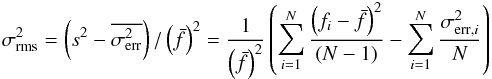 (1)from the light curve consisting of N measured fluxes fi with individual errors σerr,i and arithmetic mean
  . The normalized excess variance, or just excess variance, quotes the residual variance after subtracting the average statistical error
  from the sample variance s2 of the light-curve flux. The
  values calculated from the total light curves of our AGNs were used in S15 and are available at the CDS (see Appendix C of S15 for details). The error on the excess variance caused by Poisson noise alone (Vaughan et al. 2003) is well described by
  (2)where
  is the fractional variability (Edelson et al. 1990). As demonstrated by Allevato et al. (2013), there are additional error sources associated with the stochastic nature of AGN variability, red-noise leakage, the sampling pattern, and the signal-to-noise ratio of the light curves. In particular, these biases depend on the shape of the PSD (see e.g. Table 2 in Allevato et al. 2013), and therefore an excess variance measurement can systematically over- or underestimate the intrinsic variance of a light curve by a factor of a few (we refer to the discussion in Sect. 5.4).
Following the procedure in S15, we considered a source as variable in a given band if  (3)We emphasize that this is only a 1σ detection of variability. However, in this work we aim to investigate the relation of the amplitude of variability with AGN physical properties down to the lowest achievable level of variability. Using a more stringent variability threshold would dramatically limit the parameter space of MBH, Lbol and λEdd values we can probe. Finally, the quality of the measurements of our sample is generally high, as presented in Appendix A of S15.
The intrinsic variance of a light curve is defined to measure the integral of the PSD over the frequency range probed by the time series. Since the excess variance is an estimator of the fractional intrinsic variance, it is related to the PSD by  (4)with νmin = 1 /T and the Nyquist frequency νmax = 1/(2Δt) for a light curve of length T and bin size Δt, with the PSD normalized to the squared mean of the flux (Vaughan et al. 2003; González-Martín et al. 2011; Allevato et al. 2013).
3.2. Measuring  on different timescales
Although the excess variance is a variability estimator that is measured from the light-curve fluxes and the individual observing times do not appear explicitly in the calculation, the total temporal length and the sampling frequency of the light curve affect the resulting value. As described in the previous section, the excess variance estimates the integral of the variability power spectrum over the minimal and maximal temporal frequency covered by the light curve. Therefore we can probe different variability timescales by measuring the excess variance from different parts of the light curves. The total sample only contains values computed from the nightly averaged total light curves which typically consist of ~70–80 points and cover a period of aboutfour years. The light curves split into several segments with observations performed about every onetothreedays over a period of aboutthreetofourmonths, interrupted by gaps of aboutseventonine months without observations. Correspondingly, the shortest sampled timescale is on the order of a few days for the MDF04 survey, depending on weather constraints during the survey, whereas the longest timescale is aboutfour years. However, the sampling pattern of the MDF04 light curves additionally allows measuring the excess variance from the well-sampled individual segments of the light curves, consisting of typically 10–20 points that span a time interval of aboutthreetofourmonths. For each AGN we additionally calculated an excess variance value measured on timescales of months by averaging the values of the light-curve segments and propagating the  values of each considered segment. To avoid effects by sparsely sampled segments, which would lower the quality of the variability estimation, we included only the segments with more than ten observations in the averaging. The sample of variable type 1 AGNs with known physical parameters for this shorter timescale, that is, the MBH sample on timescales of months fulfilling
  , comprises 76 (gP1), 63 (rP1), 41 (iP1), and 43 (zP1) sources, respectively. The considerably smaller sample size follows from the fact that the light curve segments of many AGNs either have fewer than ten measurements or are almost flat, leading to very low and even negative values. We observe that the variability amplitude on timescales of years is on average about an order of magnitude larger than on timescales of months.
Although the observer-frame timescales covered by the light curves of our sample are very similar for each AGN, the wide redshift range encompassed by our sources leads to a variety of different rest-frame timescales. This is illustrated in Fig. 1, showing the distribution of the rest-frame observation length T of the total light curve and the average value of the light curve segments, obtained by dividing the observer-frame value by 1 + z to account for cosmological time dilation. The data of the MBH sample (gP1 band) on timescales of years and months are displayed. From this we note that the rest-frame length of the total light curve comprisesofaboutonetothreeyears for our sources, whereas the rest-frame length of the light-curve segments corresponds to timescales of aboutonetothreemonths. To reduce possible biases introduced by the spread in redshift, we additionally considered the sources of the MBH sample with redshifts between 1 <z ≤ 2 in our investigations, referred to as the “1z2_MBH sample”. On variability timescales of years, the 1z2_MBH sample contains 72 (gP1), 74 (rP1), 69 (iP1), and 56 (zP1) AGNs. The corresponding 1z2_MBH sample on timescales of months comprises 61 (gP1), 49 (rP1), 30 (iP1), and 31 (zP1) objects. In the following excess variance analysis (Sect. 4) we compare the variability properties of our sources as measured on timescales of years and months whenever applicable. For reference we display the properties of the various samples used throughout this work and how they are selected from the parent sample in Fig. 2.
 |
Fig. 1 Top panel: histogram of the rest-frame observation length of the total light curve for the year timescale MBH sample (gP1 band). Bottom panel: histogram of the rest-frame observation length (average value of the light-curve segments) for the month timescale MBH sample (gP1 band). |
 |
Fig. 2 Flowchart illustrating the selection of all samples considered in this work. Below the sample name (bold face) we list the sample size for each PS1 band in the order gP1, rP1, iP1, zP1. We also state the defining properties of each sample, such as objects with known AGN type, spectroscopic redshift (spec-z), black hole mass (MBH), bolometric luminosity (Lbol), or objects within a certain redshift range (see text for details). The two rightmost samples are introduced in Sect. 5.3. |
3.3. CARMA modeling of the power spectral density
Considering Eq. (4), modeling the PSD of a light curve provides more fundamental variability information than the integrated quantity. The shape of the PSD potentially allows gaining insight into the underlying physical processes connected to variability (Lyubarskii 1997; Titarchuk et al. 2007). To estimate the PSDs of our light curves, we applied the continuous-time autoregressive moving average (CARMA) model presented in Kelly et al. (2014). This stochastic variability model fully accounts for irregular sampling and Gaussian measurement errors. It also allows for interpolation and forecasting of light curves by modeling the latter as a continuous-time process.
A zero-mean CARMA(p,q) process for a time series  is defined as the solution of the stochastic differential equation
 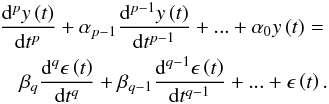 (5)It is assumed that the variability is driven by a Gaussian continuous-time white noise process
  with zero mean and variance σ2. Apart from σ2, the free parameters of the model are the autoregressive coefficients α0,..., αp − 1 and the moving average coefficients β1,..., βq. In practice, the mean of the time series μ is also a free parameter, and the likelihood function of the time series sampled from a CARMA process is calculated on the centered values
  for each light-curve point i.
The PSD of a CARMA(p,q) process is given by  (6)which forms a Fourier transform pair with the autocovariance function at time lag τ
![\begin{eqnarray} \label{eq:carmaacf} R\left(\tau\right)=\sigma^{2}\sum_{k=1}^{p}\frac{\left[\sum_{l=0}^{q}\beta_{l}r_{k}^{l}\right]\left[\sum_{l=0}^{q}\beta_{l}\left(-r_{k}\right)^{l}\right]\exp\left(r_{k}\tau\right)}{-2\mathrm{Re}\left(r_{k}\right)\prod_{l=1,l\neq k}^{p}\left(r_{l}-r_{k}\right)\left(r_{l}^{*}+r_{k}\right)}, \end{eqnarray}](/articles/aa/full_html/2016/01/aa27353-15/aa27353-15-eq71.png) (7)where
(7)where  is the complex conjugate and Re(rk) the real part of rk, respectively. The values r1,..., rp denote the roots of the autoregressive polynomial
  (8)The CARMA process is stationary if q<p and
  for all k. The autocovariance function of a CARMA process represents a weighted sum of exponential decays and exponentially damped sinusoidal functions. Since the autocovariance function is coupled to the PSD by a Fourier transform, the latter can be expressed as a weighted sum of Lorentzian functions, which are known to provide a good description of the PSDs of X-ray binaries and AGNs (Nowak 2000; Belloni et al. 2002; Belloni 2010; De Marco et al. 2013, 2015).
The CARMA model includes the Ornstein-Uhlenbeck process or the “damped random walk”, which is depicted in detail in Kelly et al. (2009) and was found to accurately describe quasar light curves in many subsequent works, as the special case of p = 1 and q = 0. Considering Eqs. (6) and (7), we note that CARMA models provide a flexible parametric form to estimate the PSDs and autocovariance functions of the stochastic light curves of AGNs. For further details on the computational methods, including the calculation of the likelihood function of a CARMA process and the Bayesian method to infer the probability distribution of the PSD given the measured light curve, we refer to Kelly et al. (2014) and the references therein.
 |
Fig. 3 Comparing the excess variance measured on timescales of years in the different PS1 bands. The data of all objects from the total sample with variability information in both considered bands are shown. The Spearman correlation coefficient and the respective p-value are reported in each subpanel. The redshift is given as a color bar. The black line corresponds to the one-to-one relation. The black error bars are the average values. |
4. Correlations of variability and AGN parameters
4.1. Wavelength dependence of the excess variance
The multiband PS1 observations of the MDF04 survey allow for an investigation of the chromatic nature of variability, that is, the dependence on the radiation wavelength. Figure 3 shows the excess variances of the total sample (variability timescale of years) for several filter pairs. The intersection of the objects with measured values in each of the two considered PS1 bands are plotted. Each subpanel displays the bluer band on the y-axis and the redder band on the x-axis, the redshift is given as a color bar. The values clearly are strongly correlated, which is also expressed by the Spearman rank order correlation coefficient ρS and the corresponding two-tailed p-value PS, giving the probability that a ρS value at least as high as the observed one could arise for an uncorrelated dataset. The ρS values quoted in each subpanel of Fig. 3 are all very close to + 1 and the respective PS values are essentially zero. However, we observe a systematic trend that the bluer bands exhibit larger variability amplitudes than the redder bands, as the respective values are shifted upward on the one-to-one relation. The offset increases when a specified blue band is compared with the series of bands with longer wavelength, that is, when comparing the pairs (gP1,rP1), (gP1,iP1) and (gP1,zP1). The variability amplitudes, however, seem to approach increasingly similar values toward the near-IR regime. The difference between the measurements of the iP1 and zP1 bands is less pronounced than the respective values of the pairs (gP1,rP1) and  . No evolution of the aforementioned wavelength dependence with redshift is observed because there are no regions that are predominantly occupied by high- or low-redshift sources in any subpanel. The same trends are observed when using the excess variance values measured on timescales of months. We emphasize that these findings agree with previous studies that observed local and high-redshift AGNs to be more variable at shorter wavelength (Edelson et al. 1990; Kinney et al. 1991; Paltani & Courvoisier 1994; di Clemente et al. 1996; Cid Fernandes et al. 1996; Vanden Berk et al. 2004; Kozłowski et al. 2010; MacLeod et al. 2010; Zuo et al. 2012).
4.2. Excess variance versus black hole mass
Determining accurate black hole masses for a large number of AGNs across the Universe is observationally expensive. However, recent works probing the high-frequency part of the PSD delivered black hole mass estimates with ~0.2–0.4 dex precision based on scaling relations of black hole mass and X-ray variability (Zhou et al. 2010; Ponti et al. 2012; Kelly et al. 2011, 2013). It is therefore important to know whether optical variability provides another independent tool for measuring black hole masses of AGNs, since massive time-domain optical surveys such as PS1 and LSST would then allow deriving black hole mass estimates for a very large number of quasars regardless of the AGN type.
In Fig. 4 we plot the gP1 band excess variance measured on timescales of years and months versus the black hole mass for the 1z2_MBH sample. Even though the estimated uncertainties of the black hole masses of our sample are large, typically ~0.25 dex, there is little evidence for any correlation between MBH and measured on timescales of years. At least for the gP1 band we observe a weak anticorrelation with MBH for variability measured on timescales of months with ρS = −0.31 and PS = 1.6 × 10⁻², but the scatter in the relation is quite large. Moreover, we do not find any significant anticorrelation relating MBH with the monthly timescale values of the remaining PS1 bands. The correlation coefficients and p-values of the 1z2_MBH sample are summarized in Table 1 for all considered PS1 bands and for both variability timescales. The correlation coefficients of the MBH sample are very similar, which is why we do not report them here. Therefore we conclude that there is no significant anticorrelation between optical variability and black hole mass for the probed variability timescales of our light curves. We stress that other optical variability studies found a correlation of variability and MBH using different variability estimators, but investigating variability timescales that are similar to those of our work. However, these results are inconsistent in the sense that several works state a positive correlation between the variability amplitude and MBH (e.g., Wold et al. 2007; Wilhite et al. 2008; MacLeod et al. 2010), whereas others report an anticorrelation with MBH (Kelly et al. 2009, 2013). Finally, we note that Fig. 4 shows no obvious dependence on redshift, and we do not observe any trend for the other PS1 bands. This is also the case for the MBH sample.
 |
Fig. 4 Excess variance (gP1 band) measured on timescales of years (top) and months (bottom) versus MBH in units of M⊙ for the 1z2_MBH sample. Spearman’s r and the respective p-value are reported in each subpanel. The redshift is given as a color bar. The black error bars correspond to the average values. |
Spearman correlation coefficient ρS and respective p-value PS of and MBH.
4.3. Excess variance versus luminosity
The existence of an anticorrelation between optical variability and luminosity has been recognized for many years, but it was often difficult to distinguish the relation from a dependency on redshift. We also observe a strong anticorrelation of the excess variance with bolometric luminosity in our dataset. The respective Spearman correlation coefficients are reported in Table 2. For the variability on timescales of years, the anticorrelation is highly significant in the gP1, rP1 and iP1 bands for the 1z2_MBH sample. On shorter variability timescales of months, the anticorrelation is even stronger and visible in all considered PS1 bands. Furthermore, we note that the anticorrelation is generally strongest for the gP1 band and is becoming less significant toward the redder bands. We stress that the anticorrelation is also detected with similar significance considering the MBH sample. Figure 5 presents the gP1 band excess variance as a function of bolometric luminosity for the 1z2_MBH sample. The figure clearly demonstrates that the anticorrelation with bolometric luminosity is apparent for both probed variability timescales and that the relation is much tighter for the shorter timescales of months.
 |
Fig. 5 Excess variance (gP1 band) measured on timescales of years (top) and months (bottom) versus Lbol in units of 1045 erg s-1 for the 1z2_MBH sample. The best-fit power law is plotted as a black solid line, the dashed lines show the 1σ errors on the fit parameters. The redshift is given as a color bar. The black error bars correspond to the average values. |
Spearman correlation coefficient ρS and respective p-value PS of and Lbol.
However, the stronger anticorrelation observed for shorter variability timescales might also be merely a selection effect, caused by considering a particular subsample of objects of the larger sample of AGNs that are varying on timescales of years. For this reason, we additionally searched for the anticorrelation with Lbol by selecting the same subsample of sources from the 1z2_MBH sample for both variability timescales. This test revealed that the observed difference in the strength of the anticorrelation for the two variability timescales is still present, with ρS = −0.45, PS = 7.2 × 10⁻⁴ (gP1 band) for variability on timescales of years, and ρS = −0.60, PS = 1.9 × 10⁻⁶ (gP1 band) for variability on timescales of months. This finding implies that regardless of the mechanism that causes the anticorrelation between the excess variance and the bolometric luminosity, it must be strongly dependent on the characteristic timescale of the variability.
To estimate the functional dependency of on Lbol, we used the Bayesian linear regression method of Kelly (2007), which considers the measurement uncertainties of the two related quantities. To do this, we fit the linear model  with Lbol,45 = Lbol/ 1045 erg s-1 to the dataset. In addition to the zeropoint β and the logarithmic slope α, this model also fits the intrinsic scatter ϵ inherent to the relation. Since the symmetric error of the excess variance given by Eq. (2) becomes asymmetric in log-space, we used a symmetrized error by taking the average of the upper and lower error. For the error of Lbol, Rosario et al. (2013) observed an rms scatter of 0.11 dex by comparing a subsample of 63 QSOs with spectra from two different datasets, whereas Lusso et al. (2011) found a 1σ dispersion of 0.2 dex for their SED-fitting method for a larger sample. In this work we performed all fits assuming a conservative average uncertainty of 0.15 dex for each AGN.
The fitted values for the 1z2_MBH sample are listed in Table 3 for each considered PS1 band, and the best-fitting model is also displayed in Fig. 5. We note that the model fits produce the same logarithmic slopes, at least within the 1σ errors, for all those PS1 bands showing a significant anticorrelation according to the ρS and PS values. A comparison of the two considered variability timescales shows that the determined slopes of the values measured on timescales of months are systematically steeper. However, within one or two standard deviations, the fitted slopes are consistent with a value of α ~ −1 for both variability timescales, indicating that the relation may be created by the same physical process2. We stress that the intrinsic scatter of the relation is only ~0.2–0.25 dex for variability on timescales of months, whereas the scatter is about a factor of two larger for variability on timescales of years. Fitting the linear model to the MBH sample, that is, including the full redshift range, results in very similar slopes for variability measured on timescales of months. But the presence of some high redshift outliers in the larger sample with measured on timescales of years drives the fitting routine toward much flatter slopes of α ~ −0.5. Finally, we tested that the anticorrelation between and Lbol is also recovered when applying a 3σ cut in the variability detection (see Eq. (3)). For the gP1 band 1z2_MBH sample, we then obtain ρS = −0.58 and PS = 1.3 × 10⁻⁷ with fitted parameters of α = −0.85 ± 0.16, β = −1.15 ± 0.12, and ϵ = 0.35 ± 0.04 for timescale variability of years. The corresponding values for timescale variability of months read ρS = −0.69 and PS = 2.2 × 10⁻⁵ with fitted parameters of α = −1.27 ± 0.22, β = −1.57 ± 0.14, and ϵ = 0.16 ± 0.06.
Scaling of with Lbol.
Several authors observed an anticorrelation of and luminosity and argued that this relation may be a byproduct of a more fundamental anticorrelation of and MBH seen at frequencies above νbr in X-ray studies, since the more luminous sources tend to be the more massive systems (e.g., Papadakis 2004; Ponti et al. 2012). This was also proposed by Lanzuisi et al. (2014), who studied the low-frequency part of the X-ray PSD, because of the very similar slopes they found for the anticorrelations of with MBH and X-ray luminosity. To determine whether there is a similar trend in our data, we display the black hole mass as color code in Fig. 6, which otherwise shows the same information as the upper panel of Fig. 5. The rough proportionality of Lbol and MBH is apparent in the color code as a weak trend that MBH increases in the x-axis direction. For the y-axis direction we observe low- and high-mass systems at the same level of variability amplitude. This is also the case for measured on timescales of months (not shown here). However, if the anticorrelation of and Lbol were caused by a hidden anticorrelation with MBH, then the less massive AGNs would predominantly occupy the upper region of the plot, and vice versa. Given that Lbol ∝ Ṁ, where Ṁ denotes the mass accretion rate, these findings suggest that the fundamental AGN parameter determining the optical variability amplitude is not the black hole mass, but the accretion rate.
4.4. Excess variance versus redshift
In the relations presented above we do not observe any strong evolution with redshift. By correlating the excess variance with the redshift of our AGNs, we find no significant dependency in any band; this is summarized in Table 4. However, we can predict the expected evolution of the variability amplitude with redshift in view of the scaling relations outlined in the previous sections.
Spearman correlation coefficient ρS and respective p-value PS of and z.
Since we observe our sources in passbands with a fixed wavelength range, the actual rest-frame wavelength probed by each filter is shifted to shorter wavelength for higher redshift. Towards higher redshift we therefore probe UV variability in the bluest PS1 bands, whereas the redder bands cover the rest-frame optical variability of the AGNs. But we showed in Sect. 4.1 that the variability amplitude generally decreases with increasing wavelength for our sources. Assuming that the intrinsic variability does not change dramatically from one AGN to another, we would therefore expect to observe a positive correlation of the excess variance with redshift for the same band. However, we found strong evidence that the intrinsic variability amplitude of AGNs is anticorrelated with bolometric luminosity. The weak selection effect apparent in Fig. A.1 shows that we actually observe the most luminous objects predominantly at higher redshift. From this selection effect alone we would expect an anticorrelation between the excess variance and redshift. The fact that we do not find a dependency of variability on redshift for our AGN sample is most likely the result of the superposition of the two aforementioned effects, which are acting in different directions. This explanation agrees with what we observe in Fig. 7, displaying the excess variance versus redshift and the bolometric luminosity as a color bar. The slight anticorrelation of with redshift is counterbalanced by a positive correlation, which is visible in various stripes of constant luminosity showing an increasing variability amplitude. The positive correlation of the variability amplitude with redshift as a result of the redshift-dependent wavelength probed by a given filter was also observed in earlier works (Cristiani et al. 1990, 1996; Hook et al. 1994; Cid Fernandes et al. 1996). Our results also agree with recent studies that did not find any significant evolution of variability with redshift or identified an observed correlation to be caused by the aforementioned selection effects (MacLeod et al. 2010; Zuo et al. 2012; Morganson et al. 2014). Finally, the low intrinsic scatter in the relation with Lbol suggests that biases due to the broad redshift distribution of our sample are negligible compared to the strong dependence on Lbol.
 |
Fig. 7 Excess variance (gP1 band) measured on timescales of months versus redshift for the MBH sample. The bolometric luminosity is given as a color bar. |
4.5. Excess variance versus Eddington ratio
The last fundamental AGN parameter for which we can probe correlations with variability is the Eddington ratio. The correlation coefficients and p-values suggest an anticorrelation between and λEdd with high significance for both studied variability timescales in the MBH and the 1z2_MBH sample. The values for the 1z2_MBH sample are quoted in Table 5. However, the relation is not as tight as the one with bolometric luminosity, but the uncertainty of λEdd is considerably larger because the errors of Lbol and MBH both contribute to its value. The 1σ dispersion of the black hole masses is 0.24 dex according to Rosario et al. (2013), but the actual uncertainty might be even larger due to systematic errors. The anticorrelation is apparent for all considered PS1 bands, although it is less robust for the zP1 band. Moreover, comparing the two variability timescales, we find the anticorrelation to be more significant for the values measured on timescales of years, in contrast to what is observed in the relation with Lbol. However, given the comparably large uncertainties of the λEdd values, this difference should not be overinterpreted. In addition, we checked that the ρS and PS values obtained for the same subsample of objects are very similar for both variability timescales.
Spearman correlation coefficient ρS and respective p-value PS of and λEdd.
We used the same fitting technique as described in Sect. 4.3 with a power-law model of the form  to find the scaling of with λEdd. For the error of λEdd we assumed Δlog Lbol = 0.15 and Δlog MBH = 0.25 for each AGN, added in quadrature3. The results are listed in Table 6, and we show the data with the fitted relation for the rP1 band in Fig. 8 for the 1z2_MBH sample. We note that owing to the large error bars of the Eddington ratio and the large scatter in the anticorrelation, the uncertainties of the fitted parameters are quite large. Considering those PS1 bands that exhibit a significant anticorrelation, that is, the gP1, rP1 and iP1 bands, we find logarithmic slopes very similar to those of the Lbol relation with α ~ −1 within the 1σ errors for both variability timescales. The intrinsic scatter of the relation between and λEdd is ~0.2–0.4 dex.
Scaling of with λEdd.
In contrast to the well-established anticorrelation of optical variability and luminosity, the actual dependency of the variability amplitude on the Eddington ratio is less clear, but evidence for an anticorrelation was detected in previous investigations (Wilhite et al. 2008; Bauer et al. 2009; Ai et al. 2010; MacLeod et al. 2010; Zuo et al. 2012; Kelly et al. 2013). The highly significant anticorrelations between and the quantities λEdd and Lbol reported in this work strongly support the idea that the accretion rate is the main driver of optical variability.
 |
Fig. 8 Excess variance (rP1 band) measured on timescales of years (top) and months (bottom) versus λEdd for the 1z2_MBH sample. The best-fit power law and other symbols are displayed as in Fig. 5. |
5. Power spectrum analysis
We did not correct our measurements for the range in redshift covered by our sources, but the excess variance depends on the rest-frame time intervals sampled by a light curve, therefore our results may be weakly biased, although we did not find any strong trend with redshift. Furthermore, the individual segments of the MDF04 light curves used in calculating the excess variance on timescales of months do not have the same length in general, introducing further biases on these timescales. However, we can independently verify our results by applying the CARMA modeling of variability described in Kelly et al. (2014), which does not suffer from the latter problems. What is more, this model allows an in-depth study of the PSDs of our light curves and therefore provides information about the part of the PSD that is predominantly integrated by our measurements.
5.1. Fitting the CARMA model
To model our light curves as a CARMA(p,q) process, we used the software package provided by Kelly et al. (2014), which includes an adaptive Metropolis MCMC sampler, routines for obtaining maximum-likelihood estimates of the CARMA parameters, and tools for analyzing the output of the MCMC samples. Finding the optimal order of the CARMA process for a given light curve can be difficult, and there are several ways to select p and q. Following Kelly et al. (2014), we chose the order of the CARMA model by invoking the corrected Akaike Information Criterion (AICc; Akaike 1973; Hurvich & Tsai 1989). The AICc for a time series of N values y = y1,...,yN is defined by  (9)with k the number of free parameters, p(y | θ) the likelihood function of the light curve, and θmle the maximum-likelihood estimate of the CARMA model parameters summarized by the symbol θ. The optimal CARMA model for a given light curve minimizes the AICc. For each pair (p,q) the CARMA software package of Kelly et al. (2014) finds the maximum-likelihood estimate θmle by running 100 optimizers with random initial sets of θ and then selects the order (p,q) that minimizes the AICc for the optimized θmle value.
Before applying the CARMA model, we transformed the light curve of each of our objects to the AGN rest-frame according to ti,rest = (ti,obs − t0,obs) /(1 + z), with t0,obs denoting the starting point of the light curve. For each source we then found the order (p,q) of the CARMA model by minimizing the AICc on the grid p = 1,...,7, q = 0,...,p − 1. With the optimal CARMA(p,q) model, we ran the MCMC sampler for 75 000 iterations with the first 25 000 discarded as burn-in to obtain the PSD of the CARMA process for each of our sources4. This procedure was performed for the flux light curves of the total sample in the four PS1 bands gP1, rP1, iP1 and zP1.
5.2. Quantifying the model fit
As outlined in Kelly et al. (2014), the accurateness of the CARMA model fit can be tested by investigating the properties of the standardized residuals χi. The latter are given by 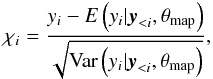 (10)where y<i = y1,...,yi − 1 and θmap is the maximum a posteriori value of the CARMA model parameters. The expectation value
  and variance Var
 of the light curve point yi given all previous values under the CARMA model are calculated using the Kalman filter (Jones & Ackerson 1990), see also Appendix A of Kelly et al. (2014). If the Gaussian CARMA model provides an adequate description of a light curve, then the χi should follow a normal distribution with zero mean and unit standard deviation. Moreover, the sequence of χ1,...,χN should resemble a Gaussian white noise sequence, that is, the autocorrelation function (ACF) at time lag τ of the sequence of residuals should be uncorrelated and be normally distributed with zero mean and variance 1 /N. Likewise, the sequence of
  should also be a Gaussian white noise sequence with an ACF distribution of zero mean and variance 1 /N.
 |
Fig. 9 In both subpanels starting from top left: a) gP1 band flux light curve (in units of 3631 Jy times 108) with the solid blue line and cyan regions corresponding to the modeled light curve and 1σ error bands given the measured data (black points). b) Standardized residuals (black points) and their histogram in blue, overplotted with the expected standard normal distribution (orange line). c) and d) autocorrelation functions (ACF) of the standardized residuals (bottom left) and their square (bottom right) with the shaded region displaying the 95% confidence intervals assuming a white noise process. The top four panels show the data of the AGN with XID 2391 that is best fit by a CARMA(3,0) process. The bottom four panels show data of the AGN with XID 30 that is best fit by a CARMA(2,0) process. |
 |
Fig. 10 Power spectral densities derived from CARMA model fits to the gP1 band flux light curves for four AGNs of our sample. The solid black line corresponds to the maximum-likelihood estimate of the PSD assuming the chosen CARMA model (selected by minimizing the AICc), the blue region shows the 95% confidence interval. The horizontal lines denote the approximate measurement noise level of the data, estimated by |
For each of our sources we visually inspected the three properties of the residuals. We found that more than 90% of the AGN light curves of our sample do not exhibit strong deviations from the expected distributions of the residuals in any of the four studied bands. We show the interpolated gP1 band flux light curve, the distribution of the residuals and the distributions of the ACF of the sequence of residuals and their square in Fig. 9 for two AGNs of our sample. The AGN with XID 2391 (upper panel of Fig. 9) is best modeled by a CARMA(3,0) process according to the minimization of the AICc. There is no evidence for a deviation from a Gaussian CARMA process because the residuals closely follow the expected normal distribution and the sample autocorrelations of the residuals and their square lie well within the 2σ interval for all but one time lag. In contrast, the AGN with XID 30 (lower panel of Fig. 9), which is best fit by a CARMA(2, 0) process, slightly deviates from the expected distribution. Since the histogram of the residuals is significantly narrower than the standard normal, a Gaussian process may not be the best description for this light curve. The light curve indicates weak periodic behavior, which may cause the difference from the normal distribution. However, the observed periodicity is probably a coincidence as a result of the irregular sampling pattern, and in fact the PSD of this source does not show any signature of a quasi-periodic oscillation (QPO). Nonetheless, the data suggest that the autocorrelation structure is correctly described by the CARMA model for this object.
In general, we observe that the CARMA model performs more poorly for the light curves of our sample that have fewer than ~40 data points. Additionally, light curves exhibiting a long-term trend of rising or falling fluxes that is not reversed within the total length of the observations also deviate somewhat from the Gaussian distribution of the residuals. In the following analysis we exclude sources revealing very strong deviations from a Gaussian white noise process. Finally, we also tested the CARMA model using the magnitude light curves of our AGNs, that is, modeling the log of the flux. We found, however, that in this case the residuals deviate more strongly from a Gaussian white noise process for many more sources than using the flux light curves. Therefore we only present the results obtained with fluxes throughout this work.
5.3. Optical PSD shape
Following the procedure described in Sects. 5.1 and 5.2, we derived the optical PSDs for the objects of the total sample in four PS1 bands, removing those sources from our sample that exhibit significant deviations from a Gaussian white noise process. The shape of the modeled PSDs resembles a broken power law for all of our sources. In Fig. 10 we display four representative gP1 band PSDs of our sample together with the error bounds containing 95% of the probability on the PSD. Since the modeled PSD should not be evaluated down to arbitrarily low variability amplitudes, we show two estimates of the level of measurement noise in our data. The gray line in Fig. 10 corresponds to the value of  , where ⟨ Δt ⟩ and
  are the average sampling timescale and measurement noise variance. Because of the large gaps between the well-sampled segments of our light curves, the median may give a better estimate, and the red line in Fig. 10 indicates the value of
  .
.
We find that most of our sources are best described by a CARMA(2,0) process (detailed fractions are given below for the final sample we consider for the remaining paper), meaning that the preferred model PSD is simply given by 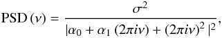 (11)which only depends on the variance of the driving Gaussian white noise process and the first two autoregressive coefficients. This PSD may be interpreted in terms of the equivalent expression of a sum of Lorentzian functions, where the roots rk of the autoregressive polynomial determine the widths and centroids of the individual Lorentzians (see Kelly et al. 2014 for details). However, in this work we aim to compare our results directly with previous studies parametrizing the PSD as a broken power law of the form
  (12)with some amplitude A, the break frequency νbr, a low-frequency slope γ1, and a high-frequency slope γ2. We fit this model to our derived PSDs using the Levenberg-Marquardt-Algorithm. For some of our objects the uncertainties on the PSD are so large that the broken power law fit is very poorly defined. Therefore we visually inspected every power-law fit and removed the sources from our sample for which the fit failed completely or was of low quality. During the fitting process we only considered the values above the noise level . In this way, we were able to determine the parameters of Eq. (12) with acceptable quality for 156 (gP1), 144 (rP1), 124 (iP1), and 93 (zP1) sources of the total sample, and in the following we refer to this sample as the “PSD sample”. For reference we show one of these model fits as a red dashed line in Fig. 11 for the AGN with XID 375.
With the chosen model order we find that 72% (gP1), 78% (rP1), 70% (iP1), and 65% (zP1) of the AGNs of the PSD sample are best fit by a CARMA(2,0) process. This may explain why many researchers found that the next-simpler model of a CARMA(1,0) process, corresponding to a damped random walk, provides a very accurate description of optical AGN light curves (Kelly et al. 2009; Kozłowski et al. 2010; MacLeod et al. 2010; Andrae et al. 2013). For 23% (gP1), 20% (rP1), 23% (iP1), and 30% (zP1) the order (3,0) minimized the AICc, and the few residual sources of the PSD sample are best described by higher orders of (3,1), (3,2), (4,1) or even (6,0), for example.
Of the objects in the PSD sample, 89 (gP1), 79 (rP1), 72 (iP1), 55 (zP1) have known black hole masses, bolometric luminosities, and Eddington ratios, hereafter termed “PSD_MBH sample”. Figure 2 summarizes these two samples, which are used throughout the PSD analysis.
 |
Fig. 11 Same as Fig. 10 in log–space for the AGN with XID 375. The red dashed line is the best-fit broken power law (Eq. (12)). Only the values above the red horizontal line were included in the fit. |
 |
Fig. 12 Distributions of the fitted break timescale (top panel), the low-frequency PSD slope γ1 (middle panel), and the high-frequency PSD slope γ2 (bottom panel). We show the data of the PSD sample, obtained with the gP1 band flux light curves. |
In Fig. 12 we present the distributions of the break timescale Tbr = 1 /νbr, the low-frequency slope γ1, and the high-frequency slope γ2 for the gP1 band objects of the PSD sample. The break timescale exhibits a distribution of timescales ranging from about ~100 days to ~300 days with a mean value of 175 days. We note that very similar characteristic timescales for optical quasar light curves have been reported by researchers using the damped random walk model (Kelly et al. 2009; MacLeod et al. 2010). However, the range of our Tbr values is quite narrow, whereas Kelly et al. (2009) and MacLeod et al. (2010) also observed characteristic timescales of several tens of days and several years for their objects. In addition, we find that the low-frequency slope γ1 is close to a value of −1 for most of our sources. The sample average is −1.08 (gP1), −1.11 (rP1), −1.17 (iP1), and −1.21 (zP1) with a sample standard deviation of 0.31 (gP1), 0.32 (rP1), 0.37 (iP1), and 0.33 (zP1). However, in order for the total variability power to stay finite, there must be a second break at lower frequencies after which the PSD flattens to γ1 = 0. A flat low-frequency PSD is still possible within the 2σ or 3σ regions of the maximum likelihood PSD for many of our objects. Furthermore, we observe a wide range of high-frequency slopes γ2 showing no clear preference with values between ~−2 and ~−4. This result suggests that optical PSDs of AGNs decrease considerably steeper than the corresponding X-ray PSDs at high frequencies, which are typically characterized by a slope of −2. This agrees with recent results obtained with high-quality optical Kepler light curves, yielding high-frequency slopes of −2.5, −3, or even −4 (Mushotzky et al. 2011; Edelson et al. 2014; Kasliwal et al. 2015). What is more, the distributions of γ1 and γ2 reveal significant deviations from the simple damped random walk model, which is characterized by a flat PSD at low frequencies and a slope of −2 at high frequencies. We emphasize that we fit very similar parameters of the broken power law in all four studied PS1 bands. This is consistent with the fact that our light curves vary approximately simultaneously in all PS1 bands, with time lags of a few days at most. The latter result is supported by a cross-correlation function (CCF) analysis we performed with our light curves using the standard interpolation CCF method (Gaskell & Sparke 1986; White & Peterson 1994). A comparison of the fitted parameters in the different PS1 bands is depicted in Appendix B.
5.4. Comparison of and the integrated PSD
The excess variance is defined to measure the integral of the PSD over the frequency range covered by a light curve (see Eq. (4)), therefore it is interesting to compare the measurement with the value of the integrated CARMA PSD for each object. This allows for a consistency test of the two variability methods.
We integrated each rest-frame PSD within the limits νmin = 1 /T and νmax = 1/(2median(Δt)), where T is the rest-frame light-curve length and median(Δt) the median rest-frame sampling timescale. First of all, we checked that integrating the maximum-likelihood estimate of the PSD (black curve in Fig. 11) and the fitted broken power law PSD (red dashed curve in Fig. 11) yield consistent results. Denoting the integral of the maximum-likelihood estimate of the PSD by  and the integral of the fitted broken power law PSD by
  , we find an average value of
  with a standard deviation of 1.2 × 10⁻⁴ for the 156 sources of the gP1 band PSD sample. In contrast, as displayed in Fig. 13, there is a systematic offset for the same objects upward of the one-to-one relation, with a slight tilt with respect to the latter comparing with the excess variance () calculated after Eq. (1). We observe that is on average a factor of ~2–3 larger than for our sources.
Part of this difference may be explained by noting that the CARMA model light-curve fits tend to omit outlier measurements in our light curves (see, e.g., Fig. 9), whereas all outliers contribute to the value of the excess variance. Moreover, as shown by Allevato et al. (2013), is a biased estimator of the intrinsic normalized source variance. The authors observed that an excess variance measurement of sparsely sampled light curves differs from the intrinsic normalized variance by a bias factor of 1.2, 1.0, 0.6, 0.3, and 0.14 for an underlying PSD with a power law slope of −1, −1.5, −2, −2.5, and −3, respectively5. However, they did not study the case of a broken power law PSD. All of our sources exhibit a broken power law PSD with a low-frequency slope of ~−1 and a high-frequency slope ranging between −2 and −4, which leads to expecting an average bias factor somewhere between ~0.3–1.0 for a value that is integrating the bend of the PSD for sparsely sampled light curves. This may be another reason for the factor of ~2–3 difference between our measurements and the values suggested by the CARMA PSDs. Finally, we point out that integrating the curve corresponding to the 2σ upper error bound of the PSD increases the integral by a factor of ~2 on average. Therefore the excess variance, which does not rely on any statistical property of the light curve, and the rather complex CARMA method yield consistent variability measurements at least within the 95% error on the PSD.
 |
Fig. 13 Comparison of the integral of the maximum-likelihood estimate of the PSD, |
5.5. Scaling of the optical break frequency
The shape of the optical PSD reported in the previous section shows that the break frequency is the most characteristic feature because it separates two very different variability regimes. For this reason, it may be possible to gain insight into the physical system at work, if this characteristic frequency scales with fundamental AGN physical properties.
Surprisingly, we do not find a statistically significant correlation of the measured break frequencies with any of the AGN parameters for the PSD_MBH sample. The Spearman rank order correlation coefficients of νbr and MBH are −0.05 (gP1), −0.24 (rP1), −0.08 (iP1), and −0.02 (zP1) with p-values of 0.61 (gP1), 0.03 (rP1), 0.52 (iP1), and 0.91 (zP1). Similarly, correlating νbr and Lbol gives ρS values of 0.23 (gP1), 0.06 (rP1), 0.10 (iP1), and 0.12 (zP1) with p-values of 0.03 (gP1), 0.61 (rP1), 0.39 (iP1), and 0.38 (zP1). Although the blue bands exhibit some evidence for a positive correlation between νbr and λEdd with large scatter, the correlation is not significant and not present considering the other bands with ρS values of 0.28 (gP1), 0.28 (rP1), 0.14 (iP1), and 0.20 (zP1) with p-values of 9.1 × 10⁻³ (gP1), 0.01 (rP1), 0.25 (iP1), and 0.15 (zP1). In Fig. 14 we plot the break frequency against these AGN parameters for the gP1 band PSD_MBH sample. Even though it is possible that there might be a hidden correlation within the large uncertainties of the involved quantities, the results obtained with the four PS1 bands suggest that such a correlation must be rather weak.
 |
Fig. 14 Optical break frequency (gP1 band PSD_MBH sample) versus MBH, color coded with Lbol (top) and λEdd, color coded with redshift (bottom). The black error bars are the average values. There is no significant evidence for a correlation with these AGN parameters. The dashed lines in the top panel correspond to the expected scaling of the orbital, thermal and viscous timescales at 10RS, see text for details. |
These findings are at odds with previous variability studies. It is well known, for example, that νbr scales inversely with MBH and may also be linearly correlated with λEdd in the X-ray bands (McHardy et al. 2006; González-Martín & Vaughan 2012). Furthermore, optical variability investigations found evidence that the characteristic timescale of the damped random walk model is correlated with MBH and luminosity (Kelly et al. 2009; MacLeod et al. 2010). Finally, if the break timescale is associated with a characteristic physical timescale of the system, we would expect a positive correlation with MBH. This follows from the fact that relevant timescales such as the light crossing time, the gas orbital timescale, and the thermal and viscous timescales of the accretion disk all increase with MBH (see, e.g. Treves et al. 1988). For reference, the dashed lines in the top panel of Fig. 14 show the frequency scaling with MBH for the orbital torb ~ 3.3(R/ 10RS)3/2(MBH/ 108M⊙), thermal tth = α-1torb, and viscous tvis = (H/R)2tth timescale assuming a viscosity parameter of α = 0.1 and a ratio of the disk scale height to radius of H/R = 0.1 at a distance of 10RS, where RS denotes the Schwarzschild radius. Although the derived Tbr values of our sample seem to be uncorrelated with MBH, the magnitude of the timescales are roughly consistent with tth at some 10RS (we recall that the gP1 band data shown in Fig. 14 are rest-frame UV data for the majority of objects). We stress, however, that the parameter space of our sample covers only a small range in frequencies, and it may be possible that a correlation appears for a much larger sample of objects spanning a wide range of values.
Scaling of PSDamp with Lbol and λEdd.
5.6. Scaling of the optical PSD amplitude
Another important characteristic of the PSD is its normalization, stating the amplitude of the PSD for each source. We tested for correlations of the PSD amplitude, which is given by PSDamp = Aνbr, with the fundamental AGN parameters MBH, Lbol and λEdd using the PSD_MBH sample. As was observed for our excess variance measurements, there is no significant correlation between the variability amplitude and the black hole mass. Spearman’s r for PSDamp and MBH reads −0.02 (gP1), 0.07 (rP1), 0.08 (iP1), and 0.00 (zP1) with p-values of 0.82 (gP1), 0.56 (rP1), 0.50 (iP1), and 1.0 (zP1). However, we find very significant evidence that PSDamp is anticorrelated with Lbol and λEdd for all of the four studied PS1 bands. The ρS and PS values of PSDamp and Lbol are −0.39 (gP1), −0.41 (rP1), −0.47 (iP1), and −0.41 (zP1) and 1.3 × 10⁻⁴ (gP1), 1.8 × 10⁻⁴ (rP1), 3.2 × 10⁻⁵ (iP1), and 2.1 × 10⁻³ (zP1), respectively. The anticorrelation is even more significant for PSDamp and λEdd with ρS values of −0.39 (gP1), −0.45 (rP1), −0.50 (iP1), −0.45 (zP1) and p-values of 1.5 × 10⁻⁴ (gP1), 2.7 × 10⁻⁵ (rP1), 7.5 × 10⁻⁶ (iP1), 6.5 × 10⁻⁴ (zP1). We point out that these results represent an entirely independent verification of the correlations we found using the excess variance as variability estimator.
In the same way as done for the excess variance, we performed a linear regression fit of the form log PSDamp = β + αlog x + ϵ for each PS1 band with x = Lbol,λEdd. The fitted values of the slope, zero-point, and intrinsic scatter are summarized in Table 7. The linear regressions obtained for the iP1 band are displayed in Fig. 15 together with the data. We note that our data suffer from few fatal outliers, showing significant deviations from the bulk of the data points. These are preferentially associated with high-redshift sources that may have low-quality Lbol and λEdd measurements or with objects whose residuals indicate some level of deviations from a Gaussian white noise process. However, we found that the presence of these few fatal outliers generally causes the slope of our fitted correlations to flatten. Therefore the slopes of the gP1, rP1 and zP1 band relations of PSDamp and Lbol listed in Table 7 are considerably shallower than the iP1 band slope, because the data of the latter are less affected by outliers. This is also true for the slopes of the gP1 and rP1 band considering the scaling of PSDamp with λEdd. After we removed the few fatal outliers from our sample, the fitted slopes are more similar for the different PS1 bands. The slopes then read −0.45 ± 0.13 (gP1), −0.73 ± 0.18 (rP1), −1.01 ± 0.23 (iP1), and −0.94 ± 0.31 (zP1) for the PSDamp–Lbol relation and −1.18 ± 0.35 (gP1), −1.27 ± 0.24 (rP1), −1.45 ± 0.35 (iP1), and −1.11 ± 0.38 (zP1) for the PSDamp–λEdd relation, respectively. We stress that these values are consistent with the slopes obtained by relating the excess variance with these quantities (see Tables 3 and 6) and suggest a common value of α ~ −1.
 |
Fig. 15 PSD amplitude (iP1 band PSD_MBH sample) versus λEdd (top) and Lbol (bottom). The redshift is given as a color bar. The best-fit power law and other symbols are displayed as in Fig. 5. |
5.7. Scaling of the high-frequency PSD slope
Finally, we observe a weak tendency for the high-frequency slope γ2 of the optical PSD to scale inversely with MBH and Lbol. This would imply that high-frequency variability is increasingly suppressed in higher mass systems. We show the scaling of the gP1 band slope γ2 with MBH in Fig. 16. Obviously, there are many outliers and the scatter in the relation is very large. Furthermore, these anticorrelations are statistically significant only in the blue PS1 bands and essentially disappear in the red PS1 bands. Spearman’s r of γ2 and MBH for the PSD_MBH sample is given by −0.42 (gP1), −0.36 (rP1), −0.30 (iP1), and −0.11 (zP1) with p-values of 3.4 × 10⁻⁵ (gP1), 1.1 × 10⁻³ (rP1), 1.1 × 10⁻² (iP1), and 0.42 (zP1). The corresponding values of ρS for γ2 and Lbol are −0.41 (gP1), −0.26 (rP1), −0.02 (iP1), and −0.10 (zP1) with p-values of 7.1 × 10⁻⁵ (gP1), 2.0 × 10⁻² (rP1), 0.85 (iP1), and 0.47 (zP1). We note that the high-frequency part of the PSD mostly covers low-variability amplitudes close to the estimated noise level. For this reason the uncertainty on the high-frequency PSD is quite large for many of our sources, leading to poorly defined γ2 values. Therefore it may well be that these anticorrelations are only a coincidence and are not present for a much larger sample.
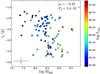 |
Fig. 16 High-frequency PSD slope γ2 (gP1 band PSD_MBH sample) versus black hole mass. The bolometric luminosity is given as a color bar. The black error bars are the average values. |
Nevertheless, the anticorrelation between γ2 and MBH is clearly apparent when we graphically compare the high-frequency PSD for three different bins of black hole mass, as shown in Fig. 17. This figure presents the median high-frequency PSD for each MBH bin after properly scaling the PSD to the value at νbr. In this way, the PSD of each object is mapped to the same unit scale, and we can take the median at every frequency to obtain a typical PSD for each black hole mass bin. As it can be seen from Fig. 17 the slope of the median PSD is systematically steeper for higher mass systems, as suggested by the distribution of the fitted slopes displayed in Fig. 16. Future studies, using much larger samples, may be able to validate the observed anticorrelation.
 |
Fig. 17 High-frequency PSD (gP1 band PSD_MBH sample) for three bins of black hole mass. We show the sample median for each MBH bin after normalizing the PSD to the values at νbr in order to transform the PSD of each AGN to the same unit scale. |
6. Discussion
The power spectrum analysis performed in this work indicates that the optical PSD of AGNs can be described by a broken power law with a low-frequency slope of γ1 ~ −1 and a high-frequency slope γ2 ranging from −2 to −4 with no preferred value. The characteristic bend in the PSD occurs at a break timescale between ~100 and ~300 days for our objects. We note that these values are higher than the expected X-ray break timescales of our sources. According to the scaling relation  reported by McHardy et al. (2006), the X-ray break timescales for the sample average of ⟨ λEdd ⟩ = 0.15 and log MBH = 7,8, and 9 are ~0.3, 3, and 30 days, whereas for the sample average mass ⟨ log MBH ⟩ = 8.5 and λEdd = 0.01, 0.1, and 1 they read ~120, 12, and 1.2 days, respectively. Furthermore, we observe that the PSD amplitude scales inversely with Lbol ∝ Ṁ with a logarithmic slope of ~−1. Assuming the power law PSD of Eq. (12), we can predict the expected scaling of the excess variance by performing the integral according to Eq. (4), giving three different cases depending on the integration limits
 ![\begin{eqnarray} \label{eq:rmspsd} \sigma_{\rm rms}^{2}\propto \begin{cases} \dot{M}^{-1}\frac{\nu_{\rm br}^{-\left(\gamma_{2}+1\right)}}{\gamma_{2}+1}\left(\nu_{\rm max}^{\gamma_{2}+1}-\nu_{\rm min}^{\gamma_{2}+1}\right), & \nu_{\rm min}>\nu_{\rm br} \\ \dot{M}^{-1}\left[\ln\left(\frac{\nu_{\rm br}}{\nu_{\rm min}}\right)\!+\!\frac{1}{\gamma_{2}\!+\!1}\left(\left(\frac{\nu_{\rm max}}{\nu_{\rm br}}\right)^{\gamma_{2}\!+\!1}\!-\!1\right)\right], & \nu_{\rm min}<\nu_{\rm br}<\nu_{\rm max} \\ \dot{M}^{-1}\ln\left(\frac{\nu_{\rm max}}{\nu_{\rm min}}\right), & \nu_{\rm max}<\nu_{\rm br}. \end{cases} \end{eqnarray}](/articles/aa/full_html/2016/01/aa27353-15/aa27353-15-eq349.png) (13)
(13)
Given the observed break timescales of our objects, this means that measuring on timescales of one to three years corresponds to the middle case of Eq. (13), whereas calculating on timescales of one to three months we are probing the high-frequency part of the PSD (upper case of Eq. (13)). We note that due to  , we expect an anticorrelation between and Lbol regardless of the frequencies sampled by the light curve. Moreover, since we do not find any significant correlation between νbr and the AGN parameters, the different scaling of with νbr for each of the three cases of Eq. (13) does not introduce further dependencies on MBH, Lbol or λEdd. Therefore the observed relations for the excess variance are consistent with the results obtained in our PSD analysis. These findings are very different from the results of previous X-ray variability studies, however, which suggested that the observed anticorrelation between the X-ray excess variance and MBH is introduced by the relation
  (McHardy et al. 2006). We stress, however, that Ponti et al. (2012) proposed PSDamp ∝ Ṁα with α ~ −0.8, remarkably similar to the value derived in this work, in order to explain their X-ray excess variance results. We note that directly comparing our findings with the results of X-ray variability studies requires assuming a strong temporal coupling between the variability of the two spectral regimes. A fair comparison would only be possible by analyzing simultaneous X-ray and UV/optical light curves.
Many researchers found correlations between the optical variability properties and physical parameters of AGNs that are similar to those we reported here. However, to date there is no self-consistent and physically motivated explanation for all the observed scalings. Although it is possible to predict correlations between the variability amplitude and the AGN parameters (also an anticorrelation with λEdd) within the standard α-disk prescription (Shakura & Sunyaev 1973) by assuming global fluctuations of Ṁ (e.g., Zuo et al. 2012; Meusinger & Weiss 2013), the resulting scaling relations are much flatter than the observed ones. What is more, the typical timescales of optical variability are much shorter than the time needed for global changes of the mass accretion rate in the entire disk, associated with the sound crossing or viscous timescale (Courvoisier & Clavel 1991; Uttley & Casella 2014; Ruan et al. 2014; Kokubo 2015). For this reason it is unlikely that global accretion rate changes are the sole driver of optical variability.
A promising alternative may be the strongly inhomogeneous disk model proposed by Dexter & Agol (2011) in which many independent local temperature fluctuations account for the flux variability. Within this toy model the accretion disk is subdivided into N varying regions that are allowed to fluctuate according to a damped random walk with an amplitude σT about the mean temperature of the standard geometrically thin optically thick accretion disk. The total variance is proportional to N-1, and Dexter & Agol (2011) were able to explain the observed 10−20% amplitudes of optical variability for N ~ 102–103 and σT ~ 0.35–0.5 dex. However, Kokubo (2015) argued that the inhomogeneous disk model can not adequately explain the tight inter-band flux-flux correlations of optical variability, which are also present in our light curves.
Although both global mass accretion rate changes and localized temperature fluctuations can not predict all characteristics of AGN variability, it may well be that both mechanisms act in parallel. Slowly changing values of Ṁ, occurring on timescales of thousands to millions of years, regulate the global long-term accretion state of an AGN, whereas a large number of localized disk inhomogeneities may account for the observed short-term variability. Disk inhomogeneities are likely to develop in a turbulent accretion flow due to the thermal, magnetorotational, or Parker instabilities. In addition, considering that our sources are luminous quasars, the accretion disks are probably radiation pressure dominated, and therefore the radiation pressure instability may also play an important role (Blaes 2014; Uttley & Casella 2014). We observed that the variability amplitude is anticorrelated with the bolometric luminosity and the Eddington ratio. These anti-correlations may be qualitatively explained by assuming that more luminous quasars with a higher mass accretion rate develop a greater number N of disk inhomogeneities due to an enhanced radiation pressure instability, leading to a smaller total variance in flux according to the inhomogeneous disk model.
The fundamental accretion disk timescales such as the orbital, thermal or viscous timescale all depend on MBH, which makes it somewhat surprising that the optical break timescale Tbr derived in this work seems to be uncorrelated with the latter and also with the other AGN physical parameters. For a standard thin α-disk the characteristic radius for emission at wavelength λ is governed by MBH and λEdd according to  (see Frank et al. 2002). Under the assumption that most of the variable flux of a given wavelength band is emitted at Rλ and associating Tbr with the thermal timescale
  at Rλ, for instance, we find
  . Obviously, the broad redshift distribution of our sample means that a variety of different radii contribute to the radiation in a fixed broadband filter, and an investigation of the scaling of Tbr is only meaningful considering small bins of MBH, λEdd and z. Otherwise any correlation can be smeared out by the range of parameters. However, our sample is not large enough to perform such a binning in an appropriate way. On the other hand, comparing the Tbr values derived in different PS1 bands, that is, at fixed MBH, λEdd and z for each source, a possible dependence on λ would be visible. But as we show in Appendix B, Tbr seems to be on average the same for each PS1 band. If quasar accretion disks indeed consist of many small localized regions of different temperature, then the radiation at a given rest-frame wavelength originates from a wide range of radii, naturally attenuating scalings with MBH, λEdd and λ. Therefore it remains unclear which physical process defines the characteristic optical break timescale. The tight correlation of the X-ray break timescale with MBH is generally interpreted to reflect the size scale of the X-ray emitting region (Kelly et al. 2011). Since most of the X-ray luminosity is probably released within a compact region of few gravitational radii in the close vicinity of the black hole, either in a roughly spherical optically thin hot corona or at the base of a relativistic jet, the effect outlined above that may smooth out a dependence of Tbr on the size scale in the optical is probably not an issue in the X-rays.
Considering the observed anticorrelation of the rms variability amplitude with Lbol and λEdd, it is tempting to interpret these results as a representation of different accretion states in AGNs. It is well known that black hole X-ray binary (BHXRB) systems undergo state changes that are believed to be connected to different accretion flow geometries. In states with high λEdd, an optically thick disk is thought to extend down close to the black hole, giving rise to a significant thermal component in the spectrum (soft state). The soft state is characterized by low rms variability amplitudes, typically lower than ~5%. In contrast, in states with low λEdd, the disk may be replaced by an optically thin hot medium at some truncation radius, generating the observed power law hard X-ray emission (hard state; Czerny 2004; Kelly et al. 2011). During the hard state the rms variability is large, with amplitudes of up to ~30−40% (Muñoz-Darias et al. 2011). In the transition region between these two canonical states the picture is less clear and different intermediate states have been defined, such as the very high state (VHS), exhibiting a spectrum of intermediate hardness and a very high X-ray flux (see, e.g., Belloni 2010, for a review). Since the timescales associated with state transitions are assumed to increase with black hole mass, a cycle through the states is expected to last thousands or millions of years for systems with supermassive black holes. For this reason, different states may only be visible for a large sample of objects, and to date it is unclear whether AGNs show the same accretion states as BHXRBs, but similarities have been observed (see, e.g., Körding et al. 2006). Interestingly, our sample contains AGNs showing high values of Lbol and λEdd with an rms amplitude of ~5%, but also sources with low values of Lbol and λEdd with an rms amplitude of ~30%. However, our objects are mostly luminous quasars characterized by a dominant disk component, and therefore it is unlikely that some of these are in a hard state, which may rather be associated with low-luminosity AGNs (Czerny 2004; Körding et al. 2006; Blaes 2014). Nevertheless, the trends observed in this work may indicate that the less variable AGNs populate a state similar to the soft state, whereas the highly variable AGNs may be in an intermediate state between the soft and hard state.
7. Conclusions
We studied correlations between the rest-frame UV/optical variability amplitude, expressed by the excess variance, and the fundamental AGN parameters for about 90 quasars covering a wide redshift range (0.3 to 2.5) from the XMM-COSMOS survey. The excess variance was measured from the multi-epoch light curves of the Pan-STARRS1 Medium Deep Field 04 survey in the four bands gP1, rP1, iP1, and zP1 and on two different timescales of on to three months and one to three years, depending on the redshift of each source. We searched for scalings of the excess variance computed on these two timescales with wavelength, redshift, black hole mass, bolometric luminosity, and Eddington ratio. Additionally, we performed a power spectrum analysis of our optical light curves in the AGN rest-frame by using the CARMA model prescription of the PSD introduced by Kelly et al. (2014). We also tested for relations between the derived PSD parameters and the aforementioned AGN physical properties. Our main results can be summarized as follows:
-
1.
The excess variances calculated in various PS1 bands are highly correlated. This agrees with the fact that our sources vary approximately simultaneously in the different bands. The variability amplitude is observed to generally decrease with wavelength, as found in many previous studies.
-
2.
We find no significant correlation between the variability amplitude and the black hole mass, neither on timescales of years nor on timescales of months. In contrast, we observe a very strong anticorrelation between the excess variance and the bolometric luminosity for the two probed variability timescales and in all PS1 bands. The logarithmic slope of the anticorrelation is consistent with a value of −1 for both variability timescales.
-
3.
The variability amplitude is also strongly anticorrelated with the Eddington ratio in all PS1 bands. The relation with λEdd exhibits the same logarithmic slope of −1 as observed for the bolometric luminosity.
-
4.
In all of these correlations there is no significant evolution with redshift. This is understood as the result of two counter-directed selection effects related to the wavelength dependence of the variability amplitude and the anticorrelation with luminosity.
-
5.
The optical PSD of all of our sources resembles a broken power law with break timescales of between ~100 and ~300 days. The break timescales seem to be uncorrelated with the black hole mass, the bolometric luminosity, the Eddington ratio, and the radiation wavelength. This lack of correlation indicates that the optical break timescale is not associated with any of the characteristic physical timescales of the accretion disk. The low-frequency slope of the PSD is roughly consistent with a value of −1, similar to the value observed in X-ray PSDs. However, the high-frequency slope exhibits a broad distribution of values between −2 and −4, generally steeper than the high-frequency slopes of X-ray PSDs. The observed shape of the optical PSD suggests significant deviations from the PSD of the damped random walk model. Finally, we observe a weak trend that the high-frequency optical PSD slope may decrease with increasing black hole mass.
-
6.
The PSD amplitude is anticorrelated with the bolometric luminosity and the Eddington ratio. The anticorrelations are seen in all PS1 bands, and the fitted slopes for the relations with Lbol and λEdd suggest a common value of −1 after fatal outliers are removed from the sample, as observed for the excess variance. We detect no correlation between the PSD amplitude and the black hole mass. Therefore the observed correlations between the excess variance and the AGN physical parameters are consistent with the relations found in the PSD analysis. The observed scalings favor the accretion rate as the fundamental AGN parameter driving the optical variability amplitude.
We found that the assumed x-axis error strongly affects the derived slope for our fitting routine. Performing test fits with the gP1 band data yielded slopes of −0.70,−0.84,−1.00, and −1.74 using Δlog Lbol = 0.01, 0.15, 0.2, and 0.3, respectively. Larger x-axis errors therefore systematically steepen the fitted slope, and this effect is particularly strong for large errors. However, the bulk of data points clearly suggests a value of ~–1.
We also performed the fits using larger uncertainties of Δlog MBH = 0.3–0.4. However, because of the systematic steepening of the derived slopes for larger x-axis errors we reported in Sect. 4.3, these errors lead to slopes that are much steeper than the overall distribution of the data implies.
The bias factor is defined by  , with the intrinsic band normalized variance
  (see Eq. (4) in Allevato et al. 2013). The average value
  is calculated from observing 5000 simulated light curves sampled from the underlying PSD. Therefore multiplying with b yields (on average) the unbiased estimate.
Acknowledgments
The Pan-STARRS1 Surveys (PS1) have been made possible through contributions of the Institute for Astronomy, the University of Hawaii, the Pan-STARRS Project Office, the Max-Planck Society and its participating institutes, the Max Planck Institute for Astronomy, Heidelberg and the Max Planck Institute for Extraterrestrial Physics, Garching, The Johns Hopkins University, Durham University, the University of Edinburgh, Queen’s University Belfast, the Harvard-Smithsonian Center for Astrophysics, the Las Cumbres Observatory Global Telescope Network Incorporated, the National Central University of Taiwan, the Space Telescope Science Institute, the National Aeronautics and Space Administration under Grant No. NNX08AR22G issued through the Planetary Science Division of the NASA Science Mission Directorate, the National Science Foundation under Grant No. AST-1238877, the University of Maryland, and Eotvos Lorand University (ELTE) and the Los Alamos National Laboratory. We thank the anonymous referee for very beneficial comments. T.S. thanks Andrea Merloni, Phil Uttley, Brandon Kelly, Jason Dexter, Simone Scaringi and Barbara De Marco for many helpful discussions and comments.
References
- Ai, Y. L., Yuan, W., Zhou, H. Y., et al. 2010, ApJ, 716, L31 [NASA ADS] [CrossRef] [Google Scholar]
- Akaike, H. 1973, in 2nd Int. Symp. Information Theory, eds. B. N. Petrov, & F. Csaki, 267 [Google Scholar]
- Allevato, V., Paolillo, M., Papadakis, I., & Pinto, C. 2013, ApJ, 771, 9 [NASA ADS] [CrossRef] [Google Scholar]
- Andrae, R., Kim, D.-W., & Bailer-Jones, C. A. L. 2013, A&A, 554, A137 [NASA ADS] [CrossRef] [EDP Sciences] [Google Scholar]
- Arévalo, P., & Uttley, P. 2006, MNRAS, 367, 801 [NASA ADS] [CrossRef] [Google Scholar]
- Arévalo, P., McHardy, I. M., Markowitz, A., et al. 2008, MNRAS, 387, 279 [NASA ADS] [CrossRef] [Google Scholar]
- Arévalo, P., Uttley, P., Lira, P., et al. 2009, MNRAS, 397, 2004 [NASA ADS] [CrossRef] [Google Scholar]
- Bauer, A., Baltay, C., Coppi, P., et al. 2009, ApJ, 696, 1241 [NASA ADS] [CrossRef] [Google Scholar]
- Belloni, T. 2010, The Jet Paradigm, Lect. Notes Phys. (Berlin: Springer Verlag), 794 [Google Scholar]
- Belloni, T., Psaltis, D., & van der Klis, M. 2002, ApJ, 572, 392 [NASA ADS] [CrossRef] [Google Scholar]
- Blaes, O. 2014, Space Sci. Rev., 183, 21 [NASA ADS] [CrossRef] [Google Scholar]
- Breedt, E., Arévalo, P., McHardy, I. M., et al. 2009, MNRAS, 394, 427 [NASA ADS] [CrossRef] [Google Scholar]
- Breedt, E., McHardy, I. M., Arévalo, P., et al. 2010, MNRAS, 403, 605 [NASA ADS] [CrossRef] [Google Scholar]
- Brusa, M., Civano, F., Comastri, A., et al. 2010, ApJ, 716, 348 [NASA ADS] [CrossRef] [Google Scholar]
- Butler, N. R., & Bloom, J. S. 2011, AJ, 141, 93 [NASA ADS] [CrossRef] [Google Scholar]
- Caballero-Garcia, M. D., Papadakis, I. E., Nicastro, F., & Ajello, M. 2012, A&A, 537, A87 [NASA ADS] [CrossRef] [EDP Sciences] [Google Scholar]
- Cackett, E. M., Horne, K., & Winkler, H. 2007, MNRAS, 380, 669 [NASA ADS] [CrossRef] [Google Scholar]
- Cappelluti, N., Brusa, M., Hasinger, G., et al. 2009, A&A, 497, 635 [NASA ADS] [CrossRef] [EDP Sciences] [Google Scholar]
- Cartier, R., Lira, P., Coppi, P., et al. 2015, ApJ, 810, 164 [NASA ADS] [CrossRef] [Google Scholar]
- Cid Fernandes, Jr., R., Aretxaga, I., & Terlevich, R. 1996, MNRAS, 282, 1191 [NASA ADS] [CrossRef] [Google Scholar]
- Cid Fernandes, R., Sodré, Jr., L., & Vieira da Silva, Jr., L. 2000, ApJ, 544, 123 [NASA ADS] [CrossRef] [Google Scholar]
- Collier, S., & Peterson, B. M. 2001, ApJ, 555, 775 [NASA ADS] [CrossRef] [Google Scholar]
- Connolly, S. D., McHardy, I. M., Cameron, D. T., et al. 2015, ArXiv e-prints [arXiv:1502.07502] [Google Scholar]
- Courvoisier, T. J.-L., & Clavel, J. 1991, A&A, 248, 389 [NASA ADS] [Google Scholar]
- Cristiani, S., Vio, R., & Andreani, P. 1990, AJ, 100, 56 [NASA ADS] [CrossRef] [Google Scholar]
- Cristiani, S., Trentini, S., La Franca, F., et al. 1996, A&A, 306, 395 [NASA ADS] [Google Scholar]
- Czerny, B. 2004, ArXiv e-prints [arXiv:astro-ph/0409254] [Google Scholar]
- Czerny, B., Doroshenko, V. T., Nikołajuk, M., et al. 2003, MNRAS, 342, 1222 [NASA ADS] [CrossRef] [Google Scholar]
- De Cicco, D., Paolillo, M., Covone, G., et al. 2015, A&A, 574, A112 [NASA ADS] [CrossRef] [EDP Sciences] [Google Scholar]
- De Marco, B., Ponti, G., Miniutti, G., et al. 2013, MNRAS, 436, 3782 [NASA ADS] [CrossRef] [Google Scholar]
- De Marco, B., Ponti, G., Muñoz-Darias, T., & Nandra, K. 2015, MNRAS, 454, 2360 [NASA ADS] [CrossRef] [Google Scholar]
- Dexter, J., & Agol, E. 2011, ApJ, 727, L24 [NASA ADS] [CrossRef] [Google Scholar]
- di Clemente, A., Giallongo, E., Natali, G., Trevese, D., & Vagnetti, F. 1996, ApJ, 463, 466 [NASA ADS] [CrossRef] [Google Scholar]
- Edelson, R., & Nandra, K. 1999, ApJ, 514, 682 [Google Scholar]
- Edelson, R. A., Krolik, J. H., & Pike, G. F. 1990, ApJ, 359, 86 [NASA ADS] [CrossRef] [Google Scholar]
- Edelson, R., Vaughan, S., Malkan, M., et al. 2014, ApJ, 795, 2 [NASA ADS] [CrossRef] [Google Scholar]
- Falocco, S., Paolillo, M., Covone, G., et al. 2015, A&A, 579, A115 [NASA ADS] [CrossRef] [EDP Sciences] [Google Scholar]
- Frank, J., King, A., & Raine, D. J. 2002, Accretion Power in Astrophysics: 3rd edn. (Cambridge, UK: Cambridge University Press), 398 [Google Scholar]
- Gaskell, C. M., & Klimek, E. S. 2003, Astron. Astrophys. Trans., 22, 661 [NASA ADS] [CrossRef] [Google Scholar]
- Gaskell, C. M., & Sparke, L. S. 1986, ApJ, 305, 175 [NASA ADS] [CrossRef] [Google Scholar]
- George, I. M., Turner, T. J., Yaqoob, T., et al. 2000, ApJ, 531, 52 [NASA ADS] [CrossRef] [Google Scholar]
- Giveon, U., Maoz, D., Kaspi, S., Netzer, H., & Smith, P. S. 1999, MNRAS, 306, 637 [NASA ADS] [CrossRef] [Google Scholar]
- González-Martín, O., & Vaughan, S. 2012, A&A, 544, A80 [NASA ADS] [CrossRef] [EDP Sciences] [Google Scholar]
- González-Martín, O., Papadakis, I., Reig, P., & Zezas, A. 2011, A&A, 526, A132 [NASA ADS] [CrossRef] [EDP Sciences] [Google Scholar]
- Graham, M. J., Djorgovski, S. G., Drake, A. J., et al. 2014, MNRAS, 439, 703 [NASA ADS] [CrossRef] [Google Scholar]
- Green, A. R., McHardy, I. M., & Lehto, H. J. 1993, MNRAS, 265, 664 [NASA ADS] [Google Scholar]
- Gu, M. F., & Li, S.-L. 2013, A&A, 554, A51 [NASA ADS] [CrossRef] [EDP Sciences] [Google Scholar]
- Hasinger, G., Cappelluti, N., Brunner, H., et al. 2007, ApJS, 172, 29 [NASA ADS] [CrossRef] [Google Scholar]
- Hawkins, M. R. S. 2002, MNRAS, 329, 76 [NASA ADS] [CrossRef] [Google Scholar]
- Hickox, R. C., Mullaney, J. R., Alexander, D. M., et al. 2014, ApJ, 782, 9 [NASA ADS] [CrossRef] [Google Scholar]
- Hirose, S., Krolik, J. H., & Blaes, O. 2009, ApJ, 691, 16 [NASA ADS] [CrossRef] [Google Scholar]
- Hook, I. M., McMahon, R. G., Boyle, B. J., & Irwin, M. J. 1994, MNRAS, 268, 305 [NASA ADS] [CrossRef] [Google Scholar]
- Hurvich, C. M., & Tsai, C.-L. 1989, Biometrika, 76, 297 [CrossRef] [MathSciNet] [Google Scholar]
- Ivezic, Z., Tyson, A. J., Strauss, M. A., et al. 2006, in BAAS, 38, 1017 [Google Scholar]
- Jiang, Y.-F., Stone, J. M., & Davis, S. W. 2013, ApJ, 767, 148 [NASA ADS] [CrossRef] [Google Scholar]
- Jones, R. H., & Ackerson, L. M. 1990, Biometrika, 77, 721 [CrossRef] [Google Scholar]
- Kasliwal, V. P., Vogeley, M. S., & Richards, G. T. 2015, MNRAS, 451, 4328 [NASA ADS] [CrossRef] [Google Scholar]
- Kelly, B. C. 2007, ApJ, 665, 1489 [NASA ADS] [CrossRef] [Google Scholar]
- Kelly, B. C., Bechtold, J., & Siemiginowska, A. 2009, ApJ, 698, 895 [Google Scholar]
- Kelly, B. C., Sobolewska, M., & Siemiginowska, A. 2011, ApJ, 730, 52 [NASA ADS] [CrossRef] [Google Scholar]
- Kelly, B. C., Treu, T., Malkan, M., Pancoast, A., & Woo, J.-H. 2013, ApJ, 779, 187 [NASA ADS] [CrossRef] [Google Scholar]
- Kelly, B. C., Becker, A. C., Sobolewska, M., Siemiginowska, A., & Uttley, P. 2014, ApJ, 788, 33 [NASA ADS] [CrossRef] [Google Scholar]
- Kim, D.-W., Protopapas, P., Byun, Y.-I., et al. 2011, ApJ, 735, 68 [NASA ADS] [CrossRef] [Google Scholar]
- Kinney, A. L., Bohlin, R. C., Blades, J. C., & York, D. G. 1991, ApJS, 75, 645 [NASA ADS] [CrossRef] [Google Scholar]
- Kokubo, M. 2015, MNRAS, 449, 94 [NASA ADS] [CrossRef] [Google Scholar]
- Körding, E. G., Jester, S., & Fender, R. 2006, MNRAS, 372, 1366 [NASA ADS] [CrossRef] [Google Scholar]
- Kotov, O., Churazov, E., & Gilfanov, M. 2001, MNRAS, 327, 799 [NASA ADS] [CrossRef] [Google Scholar]
- Kozłowski, S., Kochanek, C. S., Udalski, A., et al. 2010, ApJ, 708, 927 [NASA ADS] [CrossRef] [Google Scholar]
- Kozłowski, S., Kochanek, C. S., & Udalski, A. 2011, ApJS, 194, 22 [NASA ADS] [CrossRef] [Google Scholar]
- Kozłowski, S., Kochanek, C. S., Jacyszyn, A. M., et al. 2012, ApJ, 746, 27 [NASA ADS] [CrossRef] [Google Scholar]
- Kozłowski, S., Onken, C. A., Kochanek, C. S., et al. 2013, ApJ, 775, 92 [NASA ADS] [CrossRef] [Google Scholar]
- Lanzuisi, G., Ponti, G., Salvato, M., et al. 2014, ApJ, 781, 105 [NASA ADS] [CrossRef] [Google Scholar]
- Lawrence, A., & Papadakis, I. 1993, ApJ, 414, L85 [NASA ADS] [CrossRef] [Google Scholar]
- Leighly, K. M. 1999, ApJS, 125, 297 [NASA ADS] [CrossRef] [Google Scholar]
- Li, S.-L., & Cao, X. 2008, MNRAS, 387, L41 [NASA ADS] [CrossRef] [Google Scholar]
- Lilly, S. J., LeBrun, V., Maier, C., et al. 2009, ApJS, 184, 218 [Google Scholar]
- Lusso, E., Comastri, A., Vignali, C., et al. 2011, A&A, 534, A110 [NASA ADS] [CrossRef] [EDP Sciences] [Google Scholar]
- Lusso, E., Comastri, A., Simmons, B. D., et al. 2012, MNRAS, 425, 623 [NASA ADS] [CrossRef] [Google Scholar]
- Lyubarskii, Y. E. 1997, MNRAS, 292, 679 [NASA ADS] [CrossRef] [Google Scholar]
- MacLeod, C. L., Ivezić, Ž., Kochanek, C. S., et al. 2010, ApJ, 721, 1014 [NASA ADS] [CrossRef] [Google Scholar]
- MacLeod, C. L., Brooks, K., Ivezić, Ž., et al. 2011, ApJ, 728, 26 [NASA ADS] [CrossRef] [Google Scholar]
- MacLeod, C. L., Ivezić, Ž., Sesar, B., et al. 2012, ApJ, 753, 106 [NASA ADS] [CrossRef] [Google Scholar]
- Markowitz, A., & Edelson, R. 2004, ApJ, 617, 939 [NASA ADS] [CrossRef] [Google Scholar]
- Markowitz, A., Edelson, R., Vaughan, S., et al. 2003, ApJ, 593, 96 [NASA ADS] [CrossRef] [Google Scholar]
- McHardy, I. M. 2013, MNRAS, 430, L49 [NASA ADS] [CrossRef] [Google Scholar]
- McHardy, I. M., Papadakis, I. E., Uttley, P., Page, M. J., & Mason, K. O. 2004, MNRAS, 348, 783 [NASA ADS] [CrossRef] [Google Scholar]
- McHardy, I. M., Koerding, E., Knigge, C., Uttley, P., & Fender, R. P. 2006, Nature, 444, 730 [NASA ADS] [CrossRef] [PubMed] [Google Scholar]
- Meusinger, H., & Weiss, V. 2013, A&A, 560, A104 [NASA ADS] [CrossRef] [EDP Sciences] [Google Scholar]
- Miniutti, G., Ponti, G., Greene, J. E., et al. 2009, MNRAS, 394, 443 [NASA ADS] [CrossRef] [Google Scholar]
- Morganson, E., Burgett, W. S., Chambers, K. C., et al. 2014, ApJ, 784, 92 [NASA ADS] [CrossRef] [Google Scholar]
- Muñoz-Darias, T., Motta, S., & Belloni, T. M. 2011, MNRAS, 410, 679 [NASA ADS] [CrossRef] [Google Scholar]
- Mushotzky, R. F., Edelson, R., Baumgartner, W., & Gandhi, P. 2011, ApJ, 743, L12 [NASA ADS] [CrossRef] [Google Scholar]
- Nandra, K., George, I. M., Mushotzky, R. F., Turner, T. J., & Yaqoob, T. 1997, ApJ, 476, 70 [NASA ADS] [CrossRef] [Google Scholar]
- Nikołajuk, M., Czerny, B., Ziółkowski, J., & Gierliński, M. 2006, MNRAS, 370, 1534 [NASA ADS] [CrossRef] [Google Scholar]
- Nowak, M. A. 2000, MNRAS, 318, 361 [NASA ADS] [CrossRef] [Google Scholar]
- O’Neill, P. M., Nandra, K., Papadakis, I. E., & Turner, T. J. 2005, MNRAS, 358, 1405 [NASA ADS] [CrossRef] [Google Scholar]
- Palanque-Delabrouille, N., Yeche, C., Myers, A. D., et al. 2011, A&A, 530, A122 [NASA ADS] [CrossRef] [EDP Sciences] [Google Scholar]
- Paltani, S., & Courvoisier, T. J.-L. 1994, A&A, 291, 74 [NASA ADS] [Google Scholar]
- Papadakis, I. E. 2004, MNRAS, 348, 207 [NASA ADS] [CrossRef] [Google Scholar]
- Pereyra, N. A., Van den Berk, D. E., Turnshek, D. A., et al. 2006, ApJ, 642, 87 [NASA ADS] [CrossRef] [Google Scholar]
- Ponti, G., Papadakis, I., Bianchi, S., et al. 2012, A&A, 542, A83 [NASA ADS] [CrossRef] [EDP Sciences] [Google Scholar]
- Predehl, P., Andritschke, R., Bornemann, W., et al. 2007, in SPIE Conf. Ser., 6686, 17 [Google Scholar]
- Press, W. H. 1978, Comm. Astrophys., 7, 103 [Google Scholar]
- Rosario, D. J., Trakhtenbrot, B., Lutz, D., et al. 2013, A&A, 560, A72 [NASA ADS] [CrossRef] [EDP Sciences] [Google Scholar]
- Ruan, J. J., Anderson, S. F., MacLeod, C. L., et al. 2012, ApJ, 760, 51 [NASA ADS] [CrossRef] [Google Scholar]
- Ruan, J. J., Anderson, S. F., Dexter, J., & Agol, E. 2014, ApJ, 783, 105 [NASA ADS] [CrossRef] [Google Scholar]
- Sakata, Y., Morokuma, T., Minezaki, T., et al. 2011, ApJ, 731, 50 [NASA ADS] [CrossRef] [Google Scholar]
- Salvato, M., Ilbert, O., Hasinger, G., et al. 2011, ApJ, 742, 61 [NASA ADS] [CrossRef] [Google Scholar]
- Schawinski, K., Koss, M., Berney, S., & Sartori, L. F. 2015, MNRAS, 451, 2517 [NASA ADS] [CrossRef] [Google Scholar]
- Schmidt, K. B., Marshall, P. J., Rix, H.-W., et al. 2010, ApJ, 714, 1194 [NASA ADS] [CrossRef] [Google Scholar]
- Schmidt, K. B., Rix, H.-W., Shields, J. C., et al. 2012, ApJ, 744, 147 [NASA ADS] [CrossRef] [Google Scholar]
- Sergeev, S. G., Doroshenko, V. T., Golubinskiy, Y. V., Merkulova, N. I., & Sergeeva, E. A. 2005, ApJ, 622, 129 [NASA ADS] [CrossRef] [Google Scholar]
- Shakura, N. I., & Sunyaev, R. A. 1973, A&A, 24, 337 [NASA ADS] [Google Scholar]
- Simm, T., Saglia, R., Salvato, M., et al. 2015, A&A, 584, A106 [NASA ADS] [CrossRef] [EDP Sciences] [Google Scholar]
- Sun, Y.-H., Wang, J.-X., Chen, X.-Y., & Zheng, Z.-Y. 2014, ApJ, 792, 54 [NASA ADS] [CrossRef] [Google Scholar]
- Titarchuk, L., Shaposhnikov, N., & Arefiev, V. 2007, ApJ, 660, 556 [NASA ADS] [CrossRef] [Google Scholar]
- Trakhtenbrot, B., & Netzer, H. 2012, MNRAS, 427, 3081 [NASA ADS] [CrossRef] [Google Scholar]
- Treves, A., Maraschi, L., & Abramowicz, M. 1988, PASP, 100, 427 [NASA ADS] [CrossRef] [Google Scholar]
- Trump, J. R., Impey, C. D., McCarthy, P. J., et al. 2007, ApJS, 172, 383 [NASA ADS] [CrossRef] [Google Scholar]
- Turner, T. J., George, I. M., Nandra, K., & Turcan, D. 1999, ApJ, 524, 667 [NASA ADS] [CrossRef] [Google Scholar]
- Ulrich, M.-H., Maraschi, L., & Urry, C. M. 1997, ARA&A, 35, 445 [NASA ADS] [CrossRef] [Google Scholar]
- Uttley, P., & Casella, P. 2014, Space Sci. Rev., 183, 453 [NASA ADS] [CrossRef] [Google Scholar]
- Uttley, P., McHardy, I. M., & Papadakis, I. E. 2002, MNRAS, 332, 231 [NASA ADS] [CrossRef] [Google Scholar]
- Uttley, P., Edelson, R., McHardy, I. M., Peterson, B. M., & Markowitz, A. 2003, ApJ, 584, L53 [NASA ADS] [CrossRef] [Google Scholar]
- Van den Berk, D. E., Wilhite, B. C., Kron, R. G., et al. 2004, ApJ, 601, 692 [NASA ADS] [CrossRef] [Google Scholar]
- Vaughan, S., Edelson, R., Warwick, R. S., & Uttley, P. 2003, MNRAS, 345, 1271 [NASA ADS] [CrossRef] [Google Scholar]
- Wanders, I., Peterson, B. M., Alloin, D., et al. 1997, ApJS, 113, 69 [NASA ADS] [CrossRef] [Google Scholar]
- White, R. J., & Peterson, B. M. 1994, PASP, 106, 879 [NASA ADS] [CrossRef] [Google Scholar]
- Wilhite, B. C., Brunner, R. J., Grier, C. J., Schneider, D. P., & van den Berk, D. E. 2008, MNRAS, 383, 1232 [NASA ADS] [CrossRef] [Google Scholar]
- Wold, M., Brotherton, M. S., & Shang, Z. 2007, MNRAS, 375, 989 [NASA ADS] [CrossRef] [Google Scholar]
- Zhou, X.-L., Zhang, S.-N., Wang, D.-X., & Zhu, L. 2010, ApJ, 710, 16 [NASA ADS] [CrossRef] [Google Scholar]
- Zu, Y., Kochanek, C. S., Kozłowski, S., & Udalski, A. 2013, ApJ, 765, 106 [NASA ADS] [CrossRef] [Google Scholar]
- Zuo, W., Wu, X.-B., Liu, Y.-Q., & Jiao, C.-L. 2012, ApJ, 758, 104 [NASA ADS] [CrossRef] [Google Scholar]
Appendix A: Scaling of the AGN parameters in our sample
To characterize our sample in view of the AGN physical properties, Fig. A.1 shows the dependence of the fundamental AGN parameters on redshift and the relations between the physical properties for the MBH sample. The quantities Lbol, λEdd and MBH do not strongly depend on the redshift, meaning that our sample does not suffer from significant selection effects. There is only a weak trend that we preferentially select the more luminous objects at higher redshifts. We note that Lbol is roughly proportional to MBH, whereas there is only a very weak positive correlation with λEdd. The Eddington ratio itself is anticorrelated with MBH. However, all these dependencies show large scatter and resemble the trends also observed in other quasar samples used to study optical variability, for instance, MacLeod et al. (2010), Zuo et al. (2012). Therefore the considered sample is not strongly biased by selection effects and covers about two orders of magnitude in the AGN physical parameters.
 |
Fig. A.1 Dependence of the quantities Lbol, λEdd and MBH on redshift (left column) and scalings between the physical quantities (right column). The object data of the gP1 band MBH sample are shown. The dashed vertical lines in the left column enclose the sources of the 1z2_MBH sample. |
Appendix B: Comparing the PSD power-law fit parameters in various PS1 bands
We determined PSDs in different optical bands by modeling the gP1, rP1, iP1, and zP1 band flux light curves of our AGN sample with a CARMA(p,q) process. Fitting the derived PSDs with a broken power law according to Eq. (12), we obtained values for the amplitude A, the break frequency νbr, the low-frequency slope γ1, and the high-frequency slope γ2. We find that the optical PSDs for the different bands are generally very similar, reflecting the fact that our AGNs vary approximately simultaneously in these bands. The fitted parameters of the power law PSD are compared for the gP1, rP1, and iP1 bands in Fig. B.1. The parameters in the various bands clearly are highly correlated and very close to the one-to-one relation, except for the slope γ2. The break frequency and the low-frequency slope exhibit no dependency on the radiation wavelength. For the amplitude A we observe that the values are systematically shifted
upward of the one-to-one relation when comparing a bluer band on the y-axis with a redder band on the x-axis. This resembles the findings presented in Sect. 4.1 using the excess variance as variability estimator, and it therefore independently confirms the result that AGNs are more variable in the bluer bands. In contrast, the high-frequency slope γ2 significantly deviates in the fitted values for the different bands. This may either indicate that the PSD is wavelength dependent at high-variability frequencies or that our fitting method is significantly less robust in determining the high-frequency slope from the data at these low-variability amplitudes. The latter is clearly the case for many of the objects located far from the one-to-one relation. The large uncertainty on the PSD at low-variability amplitudes often does not allow a firm determination of the high-frequency slope, causing the different slopes for the various PS1 bands. These statements remain qualitatively the same when comparing the fitted parameters with those obtained in the zP1 band, which is why we do not show the results here.
 |
Fig. B.1 Comparison of the fit parameters of the broken power law PSD (Eq. (12)) in various PS1 bands. The data of all objects from the PSD sample with fit parameters in both considered bands are shown. The black line corresponds to the one-to-one relation. The Spearman correlation coefficient and respective p-value are shown in each panel. |
All Tables
All Figures
|
Fig. 1 Top panel: histogram of the rest-frame observation length of the total light curve for the year timescale MBH sample (gP1 band). Bottom panel: histogram of the rest-frame observation length (average value of the light-curve segments) for the month timescale MBH sample (gP1 band). |
| In the text | |
|
Fig. 2 Flowchart illustrating the selection of all samples considered in this work. Below the sample name (bold face) we list the sample size for each PS1 band in the order gP1, rP1, iP1, zP1. We also state the defining properties of each sample, such as objects with known AGN type, spectroscopic redshift (spec-z), black hole mass (MBH), bolometric luminosity (Lbol), or objects within a certain redshift range (see text for details). The two rightmost samples are introduced in Sect. 5.3. |
| In the text | |
|
Fig. 3 Comparing the excess variance measured on timescales of years in the different PS1 bands. The data of all objects from the total sample with variability information in both considered bands are shown. The Spearman correlation coefficient and the respective p-value are reported in each subpanel. The redshift is given as a color bar. The black line corresponds to the one-to-one relation. The black error bars are the average values. |
| In the text | |
|
Fig. 4 Excess variance (gP1 band) measured on timescales of years (top) and months (bottom) versus MBH in units of M⊙ for the 1z2_MBH sample. Spearman’s r and the respective p-value are reported in each subpanel. The redshift is given as a color bar. The black error bars correspond to the average values. |
| In the text | |
|
Fig. 5 Excess variance (gP1 band) measured on timescales of years (top) and months (bottom) versus Lbol in units of 1045 erg s-1 for the 1z2_MBH sample. The best-fit power law is plotted as a black solid line, the dashed lines show the 1σ errors on the fit parameters. The redshift is given as a color bar. The black error bars correspond to the average values. |
| In the text | |
 |
Fig. 6 Same as Fig. 5 for |
| In the text | |
|
Fig. 7 Excess variance (gP1 band) measured on timescales of months versus redshift for the MBH sample. The bolometric luminosity is given as a color bar. |
| In the text | |
|
Fig. 8 Excess variance (rP1 band) measured on timescales of years (top) and months (bottom) versus λEdd for the 1z2_MBH sample. The best-fit power law and other symbols are displayed as in Fig. 5. |
| In the text | |
|
Fig. 9 In both subpanels starting from top left: a) gP1 band flux light curve (in units of 3631 Jy times 108) with the solid blue line and cyan regions corresponding to the modeled light curve and 1σ error bands given the measured data (black points). b) Standardized residuals (black points) and their histogram in blue, overplotted with the expected standard normal distribution (orange line). c) and d) autocorrelation functions (ACF) of the standardized residuals (bottom left) and their square (bottom right) with the shaded region displaying the 95% confidence intervals assuming a white noise process. The top four panels show the data of the AGN with XID 2391 that is best fit by a CARMA(3,0) process. The bottom four panels show data of the AGN with XID 30 that is best fit by a CARMA(2,0) process. |
| In the text | |
|
Fig. 10 Power spectral densities derived from CARMA model fits to the gP1 band flux light curves for four AGNs of our sample. The solid black line corresponds to the maximum-likelihood estimate of the PSD assuming the chosen CARMA model (selected by minimizing the AICc), the blue region shows the 95% confidence interval. The horizontal lines denote the approximate measurement noise level of the data, estimated by |
| In the text | |
|
Fig. 11 Same as Fig. 10 in log–space for the AGN with XID 375. The red dashed line is the best-fit broken power law (Eq. (12)). Only the values above the red horizontal line were included in the fit. |
| In the text | |
|
Fig. 12 Distributions of the fitted break timescale (top panel), the low-frequency PSD slope γ1 (middle panel), and the high-frequency PSD slope γ2 (bottom panel). We show the data of the PSD sample, obtained with the gP1 band flux light curves. |
| In the text | |
|
Fig. 13 Comparison of the integral of the maximum-likelihood estimate of the PSD, |
| In the text | |
|
Fig. 14 Optical break frequency (gP1 band PSD_MBH sample) versus MBH, color coded with Lbol (top) and λEdd, color coded with redshift (bottom). The black error bars are the average values. There is no significant evidence for a correlation with these AGN parameters. The dashed lines in the top panel correspond to the expected scaling of the orbital, thermal and viscous timescales at 10RS, see text for details. |
| In the text | |
|
Fig. 15 PSD amplitude (iP1 band PSD_MBH sample) versus λEdd (top) and Lbol (bottom). The redshift is given as a color bar. The best-fit power law and other symbols are displayed as in Fig. 5. |
| In the text | |
|
Fig. 16 High-frequency PSD slope γ2 (gP1 band PSD_MBH sample) versus black hole mass. The bolometric luminosity is given as a color bar. The black error bars are the average values. |
| In the text | |
|
Fig. 17 High-frequency PSD (gP1 band PSD_MBH sample) for three bins of black hole mass. We show the sample median for each MBH bin after normalizing the PSD to the values at νbr in order to transform the PSD of each AGN to the same unit scale. |
| In the text | |
|
Fig. A.1 Dependence of the quantities Lbol, λEdd and MBH on redshift (left column) and scalings between the physical quantities (right column). The object data of the gP1 band MBH sample are shown. The dashed vertical lines in the left column enclose the sources of the 1z2_MBH sample. |
| In the text | |
|
Fig. B.1 Comparison of the fit parameters of the broken power law PSD (Eq. (12)) in various PS1 bands. The data of all objects from the PSD sample with fit parameters in both considered bands are shown. The black line corresponds to the one-to-one relation. The Spearman correlation coefficient and respective p-value are shown in each panel. |
| In the text | |
Current usage metrics show cumulative count of Article Views (full-text article views including HTML views, PDF and ePub downloads, according to the available data) and Abstracts Views on Vision4Press platform.
Data correspond to usage on the plateform after 2015. The current usage metrics is available 48-96 hours after online publication and is updated daily on week days.
Initial download of the metrics may take a while.