| Issue |
A&A
Volume 585, January 2016
|
|
|---|---|---|
| Article Number | A43 | |
| Number of page(s) | 12 | |
| Section | Extragalactic astronomy | |
| DOI | https://doi.org/10.1051/0004-6361/201527107 | |
| Published online | 16 December 2015 | |
The imprint of rapid star formation quenching on the spectral energy distributions of galaxies
1
University of CreteDepartment of Physics,
71003
Heraklion,
Greece
2
Institute for Astronomy, Astrophysics, Space Applications and
Remote Sensing, National Observatory of Athens, 15236
Penteli,
Greece
3
Laboratoire AIM-Paris-Saclay, CEA/DSM/Irfu – CNRS – Université
Paris Diderot, CEA-Saclay, 91191
Gif-sur-Yvette,
France
4
Aix-Marseille Université, CNRS, LAM (Laboratoire d’Astrophysique
de Marseille) UMR 7326, 13388
Marseille,
France
5
European Southern Observatory, Karl-Schwarzschild-Str. 2, 85748
Garching,
Germany
6
Sterrenkundig Observatorium, Universiteit Gent,
Krijgslaan 281 S9, 9000
Gent,
Belgium
7
Unidad de Astronomía, Fac. Cs. Básicas, Universidad de
Antofagasta, Avda. U. de
Antofagasta 02800
Antofagasta,
Chile
8
Institute of Astronomy, University of Cambridge,
Madingley Road, Cambridge
CB3 0HA,
UK
9
Department of Physics and Astronomy, University College
London, Gower
Street, London
WC1E 6BT,
UK
10
Istituto di Astrofisica e Planetologia Spaziali (INAF-IAPS), via
Fosso del Cavaliere 100, 00133
Roma,
Italy
11
Centro de Astronomia e Astrofísica da Universidade de Lisboa,
Observatório Astronómico de Lisboa, Tapada da Ajuda, 1349-018
Lisbon,
Portugal
Received: 3 August 2015
Accepted: 26 October 2015
Abstract
In high density environments, the gas content of galaxies is stripped, leading to a rapid quenching of their star formation activity. This dramatic environmental effect, which is not related to typical passive evolution, is generally not taken into account in the star formation histories (SFHs) usually assumed to perform spectral energy distribution (SED) fitting of these galaxies, yielding a poor fit of their stellar emission and, consequently, biased estimate of the star formation rate (SFR). In this work, we aim at reproducing this rapid quenching using a truncated delayed SFH that we implemented in the SED fitting code CIGALE. We show that the ratio between the instantaneous SFR and the SFR just before the quenching (rSFR) is well constrained as long as rest-frame UV data are available. This SED modeling is applied to the Herschel Reference Survey (HRS) containing isolated galaxies and sources falling in the dense environment of the Virgo cluster. The latter are Hi-deficient because of ram pressure stripping. We show that the truncated delayed SFH successfully reproduces their SED, while typical SFH assumptions fail. A good correlation is found between rSFR and Hi−def, the parameter that quantifies the gas deficiency of cluster galaxies, meaning that SED fitting results can be used to provide a tentative estimate of the gas deficiency of galaxies for which Hi observations are not available. The HRS galaxies are placed on the SFR-M∗ diagram showing that the Hi-deficient sources lie in the quiescent region, thus confirming previous studies. Using the rSFR parameter, we derive the SFR of these sources before quenching and show that they were previously on the main sequence relation. We show that the rSFR parameter is also recovered well for deeply obscured high redshift sources, as well as in the absence of IR data. SED fitting is thus a powerful tool for identifying galaxies that underwent a rapid star formation quenching.
Key words: galaxies: evolution / galaxies: fundamental parameters
© ESO, 2015
1. Introduction
At low redshifts, the bimodality of galaxies in the optical-to-ultraviolet (UV) color (proxy to the star formation history (SFH), e.g., Salim et al. 2005) versus stellar-mass plane is now established and has been interpreted as evidence of star formation quenching (e.g., Strateva et al. 2001; Baldry et al. 2004, 2006; Bell et al. 2004; Gil de Paz et al. 2007). However, the origin of this quenching is still open for debate. External processes linked to the environment have been proposed as one quenching mechanism from the observation that high density environments are occupied mainly by early-type galaxies (e.g., Dressler 1980). One example of environment-driven quenching is ram pressure stripping, a process expected to take place in the dense environment of clusters.
When a galaxy moves through the hot gas with a significant speed, its gas content is being stripped out (e.g., Gunn & Gott 1972; Mori & Burkert 2000; Quilis et al. 2000; Kronberger et al. 2008; Bekki 2009; Tonnesen & Bryan 2009). This mechanism is observed in galaxies of nearby clusters, such as the Virgo and the Coma clusters (e.g., Boselli & Gavazzi 2014,and references therein), and it is known that these objects lie in the green valley and are considered, in terms of star formation, intermediates between normal star-forming disks and passive early-type galaxies (e.g., Boselli et al. 2008; Hughes & Cortese 2009; Cortese & Hughes 2009). Recently, Boselli et al. (2014b) have shown that the molecular gas is also affected by ram pressure stripping, with the most affected galaxies having, on average, a factor of ~2 less molecular gas than similar objects in the field. Furthermore, Herschel observations have shown that the dust content of Hi-deficient galaxies is also affected by the cluster environment (Cortese et al. 2010, 2012b). Thus, because of ram pressure, both the Hi and the molecular gas are stripped out, leading to a quenching of the star formation activity.
Observational evidence shows that this quenching can be rapid because it can take ram pressure about several hundred Myr to produce a typical gas-deficient cluster galaxy and less than ~1.5 Gyr to completely remove the gas (Vollmer et al. 2004, 2008, 2012; Vollmer 2009; Boselli et al. 2006, 2014b; Roediger & Brüggen 2007; Crowl & Kenney 2008; Pappalardo et al. 2010). However, other studies based on simulations and observations suggest that ram pressure could act on longer timescales rather than instantaneously (e.g., McGee et al. 2009; Weinmann et al. 2010; Haines et al. 2013, 2015). Determining the timescales over which quenching mechanisms are efficient is thus critical.
The reduction of the star formation rate (SFR) of a galaxy, whether rapid or smooth, is translated in its SFH. Thus the quenching affects the shape of the UV-to-near-infrared (NIR) emission of its stellar population. Indeed, it is well established now that the near-UV (NUV)-r color is also an excellent tracer of gas content (Cortese et al. 2011; Fabello et al. 2011; Catinella et al. 2013; Brown et al. 2015). Consequently, fitting the observed UV to NIR emission of galaxies with stellar population models convolved by assumed SFHs allows us to place constraints on the true galaxy SFH. These methods have been widely applied in the literature to retrieve key physical properties of galaxies, such as their stellar masses and SFRs.
To model a galaxy SED, it is necessary to make some assumptions about its SFH. Galaxies typically form their bulk of stars through secular process with, in addition, variations in the SFR on different timescales, such as star formation bursts (e.g., Elbaz et al. 2011; Sparre et al. 2015). Simple functional forms are usually assumed in the literature, such as an exponentially decreasing or increasing SFR, two exponential decreasing SFRs with different e-folding times, a delayed SFH, a lognormal SFH, or an instantaneous burst (e.g., Ilbert et al. 2013; Pforr et al. 2012; Lee et al. 2009; Schaerer et al. 2013; Gladders et al. 2013). These simple assumptions reproduce only smooth variations in the SFH, even though it is possible to add one or several bursts of star formation. None of these SFHs, though, can model a rapid and quite sudden quenching of star formation.
In this work, we use a new SFH analytical function to model a rapid and sudden quenching of star formation in galaxies. To evaluate this approach, we need a sample of galaxies which have experienced this rapid quenching scenario. Nearby galaxies of the Virgo cluster are known to undergo ram pressure stripping and are thus good candidates for our study. Some of these galaxies are included in the Herschel Reference Survey (Boselli et al. 2010), which benefits from a wealth of ancillary data and contains galaxies from a wide range of environments. This stripping of the gas, observed in late-type cluster galaxies, can be quantified by the Hi-deficiency. This parameter is defined as the logarithmic difference between the average Hi mass of a reference sample of isolated galaxies of similar type (from Sa to Scd-Im-BCD) and linear dimension and the Hi mass actually observed in individual objects: Hi−def= log MHiref − log MHiobs. According to Haynes et al. (1984), log h2MHiref = c + dlog (h × diam)2, where c and d are weak functions of the Hubble type, diam (in kpc) is the linear diameter of the galaxy (see Gavazzi et al. 2005; Boselli & Gavazzi 2009), and h = H0/ 100. In the following, we define as “gas-rich” or “normal” those galaxies with Hi−def≤ 0.4, and “Hi-deficient” as those with Hi−def> 0.4, following Boselli et al. (2012). Although the HRS sample was first built to study the dust properties of galaxies with Herschel, the broad photometric coverage available for these sources from UV to submm wavelengths makes it ideal for testing a new SED modeling approach.
The paper is organized as follows. We present the Herschel Reference Survey in Sect. 2 and the SED fitting code CIGALE in Sect. 3. In Sect. 4, we present the truncated SFH included in CIGALE and study the constraints that we have on its free parameters. The results of the SED fitting are presented in Sect. 5 and are discussed in Sect. 6. SED fitting is performed assuming an IMF of Salpeter (1955), but the results of this work are found to be robust against IMF choice.
2. The Herschel Reference Survey sample
To examine the impact of rapid quenching on the SED of galaxies, we used the Herschel Reference Survey (HRS, Boselli et al. 2010). The HRS is a combined volume- and flux-limited sample composed of galaxies with a distance between 15 and 25 Mpc. The galaxies are then selected according to their K-band magnitude, a reliable proxy for the total stellar mass (Gavazzi et al. 1996). The sample contains 3221 galaxies: 62 early-type and 260 late-type. The HRS covers all morphological types, so we used the classification presented in Cortese et al. (2012a).
The Hi data available for the HRS galaxies are presented in Boselli et al. (2010). They are available for 96% of the late-type galaxies of the HRS. Hi deficiencies of the HRS galaxies were measured using the calibrations of Boselli & Gavazzi (2009). The HRS galaxies have Hi−def between −0.65 and 1.69. The gas-rich galaxies serve as a comparison element to identify possible trends linked to the gas deficiency. This reference sample benefits from a wealth of ancillary data, photometry from UV to radio (Bendo et al. 2012; Cortese et al. 2012a, 2014; Ciesla et al. 2012, 2014, and from the literature), as well as optical spectra (Boselli et al. 2013, 2014a, 2015).
In this work, we have selected the HRS galaxies defined as late-type (Sa and later types), which are also detected with GALEX in the FUV and NUV, since these observations are mandatory for our study, as we discuss in Sect. 4.3. Our subsample consists of 228 galaxies, which comprise 136 normal star-forming ones and 92 that are Hi-deficient. The photometric coverage of this subsample is presented in Table 1 and is thoroughly discussed in the associated papers. Even though a direct consequence of ram pressure stripping is evident through the observed UV to NIR emission, a complete modeling of the galaxy SED, using data from the UV to the submm, is essential to quantify the current stellar emission (e.g. Buat et al. 2014).
Broad-band filter set used in this paper.
3. Modeling and fitting galaxy SEDs with CIGALE
CIGALE2 (Code Investigating GALaxy Emission) is a SED modeling software package that has two functions: a SED modeling function and a SED fitting function (Roehlly et al. 2014; Burgarella et al., in prep.; Boquien et al., in prep.). Even though the philosophy of CIGALE, originally presented in Noll et al. (2009), remains, the code has been rewritten in Python and additions have been made in order to optimize its performance and broaden its scientific applications. The SED modeling function of CIGALE allows the building of galaxy SEDs from the UV to the radio by assuming a combination of modules that model the SFH of the galaxy, the stellar emission from stellar population models (Bruzual & Charlot 2003; Maraston 2005), the nebular lines, the attenuation by dust (e.g., Calzetti et al. 2000), the IR emission from dust (Draine & Li 2007; Casey 2012; Dale et al. 2014), the AGN contribution (Fritz et al. 2006), and the radio emission. CIGALE builds the SEDs while taking the balance between the energy absorbed by dust and reemitted in the IR into account.
These modeled SEDs are then integrated into a set of filters to be compared directly to the observations. For each parameter, a probability distribution function (PDF) analysis is done. The output value is the likelihood-weighted mean value of the PDF and the associated error is the likelihood-weighted standard deviation. We used CIGALE to derive the physical properties of galaxies, such as stellar masses, instantaneous SFRs, dust attenuation, IR luminosities, and dust masses, and took panchromatic information on the SED into account.
In CIGALE, the assumed SFH can be handled in two different ways. The first is to model it using simple analytic functions (e.g., exponential forms, delayed SFHs, etc.). The second is to provide more complex SFHs, such as those provided by semi-analytical models (SAM) and simulations (Boquien et al. 2014; Ciesla et al. 2015), an approach that we do not use in the present study.
4. Truncated SFH
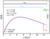 |
Fig. 1 Illustration of the truncated delayed SFH implemented in CIGALE. The purple dashed line represents a normal delayed SFH with τmain = 5 Gyr, without truncation. The red solid line is the truncated delayed SFH. |
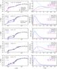 |
Fig. 2 Left column: examples of best fits obtained with CIGALE for one normal and four Hi-deficient HRS galaxies using three different SFHs assumptions: a delayed SFH (navy blue), a 2-exponentially decreasing SFH (cyan), and a truncated delayed SFH (red). Right column: for each galaxy, the output best fit SFH obtained for the three different assumptions made. |
4.1. The need for truncated SFH
Several studies have already shown that the delayed SFH matches observations, as well as SFHs obtained through SAM or hydrodynamical simulations (e.g., Boselli et al. 2001; Sparre et al. 2015; Ciesla et al. 2015). We thus base our work on the delayed SFH, which is represented with the following expression:  (1)where t is the time (t = 0 corresponds to the time when the first stars of the galaxy formed), and τmain is the e-folding time of the stellar population. As shown in Fig. 1, this SFH describes secular star formation but not any star formation burst. Stellar masses and SFR obtained through SED fitting using this SFH yield offsets less than 10%, comparable to the widely spread exponentially decreasing SFHs (with one or two stellar populations); furthermore, delayed SFH provides better estimates of the age of a galaxy unlike exponentially decreasing models, which underestimate this parameter (Maraston et al. 2010; Pforr et al. 2012; Ciesla et al. 2015)
Even though the SFH assumptions commonly used in the literature provide good fits of the stellar emission of normal galaxies, they fail to reproduce the stellar emission of rapidly quenched galaxies, such as the Hi-deficient galaxies of the HRS. Indeed, Fig. 2 shows the best fits obtained for one normal and four Hi-deficient galaxies using the delayed and, for comparison, the usual 2-exponentially decreasing SFH. The dynamical range of the parameters and their sampling are presented in Table 2.
These two models fit the data of the normal (gas-rich) galaxy (top panel) well. However, the delayed SFH model struggles to simultaneously reproduce the UV-optical observations linked to the young stellar population and the NIR data linked to the old stellar population. Furthermore, to be able to reproduce the optical-NIR data as well as the very low SFR, the delayed SFH obtained from the best fits have a low value of τmain overall (Fig. 2, right column). A delayed SFH with a low value of τmain is more characteristic of early-type passive galaxies with the creation of the bulk of the stars at early time and then a smooth decrease in the star formation activity. The 2-exponentially decreasing SFH model reproduces the UV emission better, but with the consequence of underestimating the optical data. We also explored leaving the age of the galaxy as a free parameter and do not find any change in the results shown in Fig. 2. Thus, the usually assumed SFHs fail to reproduce the peculiar UV-NIR SED of rapidly quenched galaxies such as the Hi-deficient objects.
4.2. Implementing a truncated SFH
To model the SFH of Hi-deficient galaxies, previous studies (e.g., Boselli et al. 2006; Fumagalli et al. 2011) proposed to use a delayed SFH that, at a given time, would lead to a strong decrease in the SFR. We thus include in CIGALE such a SFH, with the following expression:  (2)where ttrunc is the time when the star formation is quenched, and rSFR is the ratio between SFR(t>ttrunc) and SFR(t = ttrunc):
 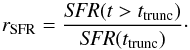 (3)Figure 1 shows an example of truncated SFH.
Galaxy parameters used in the SED fitting procedures.
The SFH is thus determined through four parameters, the age of the galaxy, the e-folding time of the main stellar population model, τmain, the age of the truncation, agetrunc, and rSFR. This model, which represents the effect of the cluster environment on galaxy SFH, is simple in order to limit the possible degeneracy that could arise from a more complex shape with additional free parameters. We discuss its validity in Sect. 6.
To understand the impact of the two parameters handling the truncation, agetrunc and rSFR on the shape of the SED, we show in Fig. 3 modeled UV-to-optical SEDs varying the truncation age (top panel) and the ratio between the SFR after and before the truncation (bottom panel). The truncation age, agetrunc, mainly affeccts the SED between 0.1 and 0.5 μm with a decrease in the emission in this range when agetrunc increases. The rSFR parameter affeccts the SED at wavelengths shorter than 0.5 μm. When the SFR after truncation is zero, the emission at λ< 0.1 μm drops significantly. Very low values of rSFR, 0.05 for instance, are sufficient to produce emission at λ< 0.1 μm, which increases with rSFR. From Fig. 3, it is clear that the GALEX filters are mandatory for constraining these two parameters, since both FUV and NUV filters probe the spectral range where they affect the SED.
 |
Fig. 3 Impact of the two parameters, agetrunc (upper panel) and rSFR (lower panel), on the SED considering a τmain of 10 Gyr. SEDs are color-coded according to the value of the free parameter. For clarity, we only show models with rSFR lower than 0.45 in this plot. At the bottom of each panel, we show the filters of GALEX (red), SDSS, and 2MASS. |
4.3. Evaluating the SFH parameters with a mock catalog
To examine if we can constrain these four parameters from broad-band SED fitting with CIGALE, as well as the accuracy and precision that we can expect, we built a mock galaxy catalog. This sort of catalog consists of theoretical SEDs, built here with CIGALE, for which we know the exact underlying physical parameters (i.e., galaxy age, complete SFH, etc.). Using our fitting procedure on this mock catalog allows us to compare the output results to the parameters used to build the mock catalog and to evaluate how well we constrain any given parameter. We used the modeling function of CIGALE to create a set of galaxy SEDs, following the method presented in Giovannoli et al. (2011). The stellar emission was computed by convolving the stellar population models of Bruzual & Charlot (2003) with the truncated delayed SFH presented in Sect. 4.2. We used the Calzetti et al. (2000) law to attenuate the stellar emission, while the IR emission was modeled with Dale et al. (2014) templates. The parameters used to compute the mock SEDs are presented in Table 2. The mock SEDs are integrated into a set of filters that correspond to the observations available for the HRS galaxies (Table 1). Following the method presented in Ciesla et al. (2015), we perturbed the mock flux densities, adding a noise randomly taken from a Gaussian distribution with σ = 0.1, and a photometric error of 15% was assumed for each flux density.
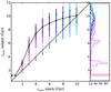 |
Fig. 4 Constraints on τmain as a result of the mock catalog analysis of the truncated SFH parameters. The dispersion of the output values are shown in blue, the mean and 64th percentile for each input values in black. The black solid line is the one-to-one relationship. The right panel shows the distribution of the points for each input value of τmain. |
We now have a set of mock SEDs for which we know the exact parameters, including the values of agetrunc and rSFR. Using the SED fitting function of CIGALE, we ran the code on the mock catalog in order to compare the output parameters to the ones we used to create the mock SEDs. The parameters used to perform the SED fitting are also presented in Table 2.
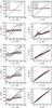 |
Fig. 5 Results of the mock catalog analysis for the two parameters agetrunc and rSFR. The five lefthand panels present the constraint on agetrunc for five different τmain (1, 3, 5, 7, and 10 Gyr). The colored lines correspond to different values of rSFR. The five right panels display the constraint on rSFR for the same five values of τmain (1, 3, 5, 7, and 10 Gyr), and the colored lines correspond to different agetrunc. In each panel, the black solid line is the one-to-one relationship. |
Figure 4 compares the output values of τmain with the true values, which were used to create the mock galaxy catalog. A perfectly recovered parameter would show a one-to-one relationship. Considering the known difficulty in recovering SFH parameters from SED fitting (e.g., Giovannoli et al. 2011), the constraint on τmain is relatively correct up to ~4 Gyr with an overestimate of a factor less than 2, but is degenerated for values higher than 4 Gyr for which the code will provide an estimate between 8 and 10 Gyr. Indeed, there is a flattening of the relation above 4 Gyr. For comparison, the mock analysis of τmain used in the delayed SFH shows slightly different behavior with values of τmain< 4 Gyr being very well constrained and higher values becoming overestimated up to 30%. It is, however, known that this parameter is difficult to constrain (e.g., Buat et al. 2014).
In a similar way to Fig. 4, Fig. 5 presents the results for agetrunc (top panels) and rSFR (bottom panels). The results are shown for different values of τmain (1, 3, 5, 7, and 10 Gyr). The agetrunc parameter is never constrained when τmain = 1 Gyr, and only for rSFR = 0 for higher values of τmain. Indeed, as shown in Fig. 3, the spectral range where agetrunc affects the SED is limited to 0.1−0.5 μm, where the rSFR also plays a role in shaping the SED. Without any additional information, it is thus difficult for the model to determine agetrunc precisely when rSFR> 0, as we can see directly in Fig. 5.
The rSFR parameter is estimated relatively well for true values of τmain ≥ 5 Gyr. However, the recovered value of τmain is biased toward higher values relative to the true value. As seen in Fig. 4, a true value of τmain ≥ 5 Gyr corresponds to a recovered value of ~8 Gyr. For low values, τmain = 1 Gyr, the results from the mock analysis show a flat relation, meaning that rSFR is not constrained. Indeed, delayed SFH with a small τmain of 1 Gyr corresponds to an early rise of the SFR at early cosmic time followed by a rapid but smooth decrease of the SFR that it is close to 0 at t = 13 Gyr. It is thus difficult to point out a rapid quenching of star formation in galaxies undergoing a smooth and long decrease of their star formation activity over several Gyr. For higher τmain, the estimate is relatively close to the true value, especially for low values of rSFR. For higher values of rSFR, the higher τmain, the better the constraint.
Thus, with the available set of filters, τmain and rSFR can be constrained relatively well for τmain ≥ 5 Gyr. To constrain agetrunc from SED fitting, additional information is needed, such as the Hα flux density. Indeed, the intensity of the Hα lines is directly linked to the number of Lyman continuum photons, and this could put a strong constraint on agetrunc as seen in the bottom panel of Fig. 3 (e.g., Lee et al. 2009; Weisz et al. 2012; Boselli et al. 2015). This is the topic of a forthcoming study (Boselli et al., in prep.).
5. Application to the HRS galaxies
5.1. Results from SED fitting
We ran CIGALE on the subsample of HRS late-type galaxies, including 136 normal and 92 Hi-deficient galaxies, and used the truncated delayed SFH for all of them. The fits are performed over the entire spectrum from the UV to the submm. Indeed, benefiting from the philosophy of CIGALE, which is based on an energy balance between UV-optical and IR, IR and submm data provide an additional constraint on the dust attenuation. The set of parameters used for the fit are presented in Table 2.
The mock analysis showed that the agetrunc parameter is not constrained from broad band photometry. Nevertheless, we performed a first run of CIGALE leaving this parameter free. The resulting distribution of agetrunc does indeed peak at the same value for both the normal and deficient subsamples and with a similar spread, confirming the difficulty of constraining this parameter (see Fig. A.1). We thus decided to fix its value to 350 Myr and performed a second run with this parameter fixed. From now on, we present and discuss the results of the run with fixed agetrunc.
Mean  obtained using the three SFHs mentioned in this work and for three bins of Hi−def.
For a normal galaxy, the quality of the fit in UV to optical is the same compared to a delayed SFH and a 2-exponentially decreasing SFH (Fig. 2, top panel). For the Hi-deficient galaxies, the truncated SFH results in better agreement between the modeled SEDs and the data. Both the FUV and NUV flux densities are reproduced by the model (Fig. 2), where other SFH assumptions failed to do so. In addition, the computed models are able to reproduce the emission of all the stellar populations, both young and old stars. Although it is complicated to compare different obtained from models with different degrees of freedom, we give in Table 3 the mean obtained for the three SFH mentioned in this work and for three bins of Hi−def. The mean obtained with normal SFHs is around three times higher for the Hi−def galaxies, whereas the truncated SFH provides consistent for all of three subsamples.
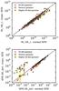 |
Fig. 6 Comparison between the stellar masses (top panel) and SFR (bottom panel) obtained using the truncated and normally delayed SFH. Normal galaxies are shown in gray, whereas Hi-deficient and highly deficient galaxies (with Hi−def≥ 1) are shown in red and yellow, respectively. The black solid lines represent the one-to-one relationship. |
The use of the truncated SFH compared to the normal delayed SFH mostly affects the UV and NIR, providing better fits (Fig. 2). Since these domains are crucial to determining the SFR and stellar mass of galaxies, we show in Fig. 6 the differences obtained on these parameters using the truncated and normal delayed SFH. For the normal galaxies, the comparison shows small scatter, but this is expected because different SFHs are used (e.g., Pforr et al. 2012; Buat et al. 2014; Ciesla et al. 2015). This small scatter increases when we consider the Hi-deficient galaxies, leading to lower stellar masses obtained with the truncated SFH and lower SFRs. The effect is more striking when considering the most deficient galaxies (with Hi−def≥ 1) where the stellar mass is overestimated by 30% and the SFR by a factor of ~15 on average when using a normal delayed SFH instead of the truncated SFH. The large difference observed in the SFR estimates can be understood from Fig. 2 where it is shown that the normal delayed SFH strongly underestimates the UV emission of the Hi-deficient galaxies. This emphasizes the importance of using an appropriate SFH to retrieve the physical parameters of galaxies.
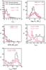 |
Fig. 7 Distribution of the output parameters obtained from the SED fitting procedure with CIGALE. The results for the normal galaxy sample are shown in gray while the results for the Hi-deficient sample are shown in red. |
The distribution of the χ2, M∗, SFR, rSFR, and τmain obtained from the SED fitting using the truncated SFH are presented in Fig. 7 for both normal and Hi-deficient galaxies. The χ2 distributions of the normal and Hi-deficient samples peak at different values, with a mean of 1.54 and 1.26, respectively. The distributions of the stellar mass of both subsamples are similar, peaking at log M∗ ≈ 9.9−10.0 and spreading from 8.5 to 11.2. However, the distribution of star formation rates of the Hi-deficient clearly shows that most of these galaxies have a very low, almost zero SFR, as expected for quenched galaxies. The distribution of the rSFR parameter shows two different behaviors for normal and deficient galaxies. The Hi-deficient subsample distribution shows lower values with 34 sources with rSFR< 0.15 out of 92 deficients galaxies. There is a second peak at 0.3 in the rSFR distribution with 16 galaxies. The rSFR distribution of normal galaxies is flat and shifted toward higher values, although not as close to one as one would expect. This can be explained from Fig. 5 where we see that, even for high values of τmain, rSFR values close to one tend to be underestimated by at least 10−20%. Finally the distribution of τmain shows that most of the sources have τmain ≥ 5 Gyr, the typical value above which the uncertainty on rSFR begins to reduce, as discussed in Sect. 4.3.
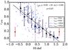 |
Fig. 8 Relation between rSFR and the Hi deficiency. Data points are color-coded according to the value of τmain obtained from the fit. The mean errors bars for each subsample are provided with the red star for the normal galaxy sample and with the red filled circle for the deficient galaxies. The Spearman correlation coefficient ρ of the relation is indicated. Black triangles are the median values in bins of ΔHi−def= 0.2, and the error bars are the standard deviation of the points in each bins. The black filled line is the best linear fit to the data. The black dotted line indicates the adopted threshold used to separate normal from deficient galaxies. |
5.2. Relation between the strength of the quenching and the HI-deficiency
To further examine the rSFR parameter, we show in Fig. 8 the relation between this parameter and Hi−def. With a Spearman correlation coefficient of −0.67, there is a good anti-correlation between these two parameters for which the best linear fit results in  (4)Indeed, galaxies with a high Hi−def parameter are the ones most affected by the cluster environment with a large portion of their gas content stripped. These sources are thus the most quenched and, consequently, have a very low rSFR value. In contrast, sources with negative values of Hi−def with no gas stripped show high values of rSFR. However, we would have expected values closer to one for normal galaxies and less dispersion. A value lower than one for the normal star-forming galaxies means that the assumption of a quasi constant SFR over the past few hundred Myr from the delayed SFH is too strong. Thus, although not equal to one, high values of rSFR may model a small decrease towards the end of the evolution in addition to the one obtained with the simple smooth, delayed SFH. From Fig. 8, we see that normal galaxies with the lowest rSFR also have a low value of τmain. From the results of the mock catalog analysis, low values of τmain lead to underestimating rSFR. To understand that the values lower than one obtained for the normal galaxies are due to underestimating high values of rSFR, as seen in the mock catalog results (Fig. 5), we derived rSFR corrections from the mock results and applied them to the rSFR values. The relation observed in Fig. 8 generally remains unchanged with a Spearman correlation coefficient of −0.66. This is because most of the sources have a τmain value higher than 5 Gyr and thus small corrections.
This relation between the two parameters can be useful because the Hi−def parameter, which quantifies the impact of the environment on the gas content of a galaxy, and even gas measurements are not available for a large number of sources, especially at high redshifts. The NUV-r color, an excellent proxy for gas content in galaxies, also shows a good correlation with Hi−def but slightly more dispersed, with a Spearman correlation coefficient of 0.61 (Fig. B.1). From SED fitting, with a wide photometric coverage, especially including the rest frame UV, it would be possible to obtain an estimate of this parameter. More generally, it means that broad band SED fitting can provide information on SFH that are recently perturbed, such as a rapid decrease in the star formation activity.
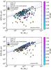 |
Fig. 9 Relation between the SFR and M∗ of the HRS subsamples. Black stars are the normal galaxies, filled circles are the Hi-deficient galaxies color-coded according to the Hi−def parameter. Yellow crosses point out the sources for which rSFR = 0. Main sequence relations found at z = 0 are shown in dashed lines: in blue the one from Ciesla et al. (2014), in red the relation of Peng et al. (2010), and the relation derived in this work is the black solid line. Top panel: observed relation obtained with CIGALE. Bottom panel: estimated positions of the Hi-deficient galaxies before interaction with the environment obtained after correcting their instantaneous SFR with the rSFR parameter. |
5.3. Position of the HI-deficient galaxies on the SFR–M∗ diagram
Recent studies of large samples of galaxies have shown that the majority of star-forming galaxies follow a SFR–M∗ correlation, which is called the main sequence (MS, Noeske et al. 2007; Elbaz et al. 2007; Peng et al. 2010; Speagle et al. 2014). Because the sample was selected in the K band to be complete in mass, the HRS galaxies are ideal to probe the MS at z = 0. In Fig. 9, we show the positions of our normal star-forming and Hi-deficient subsamples on the MS diagram. In this work, stellar masses and SFR are estimated through our SED fitting procedure. The normal galaxies are the same as those studied in Ciesla et al. (2014), who demonstrate that, using different estimates of SFRs and M∗, the gas rich late-type subsample of HRS galaxies lie on the MS derived by Peng et al. (2010), as shown in Fig. 9, but with a slightly flatter slope. The new estimates of the masses and SFRs now place the galaxies slightly lower than the MS derived in Ciesla et al. (2014) owing to the different methods employed to determine them. At lower masses, the HRS galaxies agree better with the relation determined by Peng et al. (2010), even though the slope of the MS is still flatter. With SFRs determined from new Hα imaging, Boselli et al. (2015) show that the best linear fit to their SFR-M∗ relation is closer to Ciesla et al. (2014), whereas the bisector of the relation is closer to the relation of Peng et al. (2010). Since the slope of the MS is sensitive to the methods and assumptions made to derive the SFRs and stellar masses, we do not discuss the different relations obtained by Peng et al. (2010), Ciesla et al. (2014), and Boselli et al. (2015) further because the results of this work are not linked to the MS slope.
In Fig. 9 (top panel), the galaxies with an Hi−def lower than ~1.00 seem to lie at the lowest part of the MS compared to the normal galaxies, and the most extreme deficient ones (Hi−def> 1.00) are off the MS with very low SFR compared to their stellar mass. Indeed, previous studies have shown that the Hi-deficient galaxies lie in the green valley and are considered as midway between star-forming disks and passive early-type objects (e.g., Boselli et al. 2008). Furthermore, Boselli et al. (2015) determined the SFR-M∗ relation for the normal and the Hi-deficient star-forming galaxies and find a shift of 0.65 dex between the two relations. However, using the observed SFR of these sources and the estimate of the rSFR parameter obtained from the SED fitting, we can have an estimate of the SFR of the galaxies before being affected by the dense environment of the Virgo cluster. In the bottom panel of Fig. 9, we show the positions of the Hi-deficient sources using their “corrected” SFR. After correction, almost all of the Hi-deficient galaxies lie on the MS formed by the normal star-forming galaxies of the HRS sample. Five deficient sources remain below the MS. These five sources have a rSFR equal to 0 and a very low SFR with SFR/error lower than 1.6. Given the definition of this parameter, it is not possible to obtain an estimate of the SFR of these sources before the truncation. The properties of the Hi-deficient galaxies before being affected by the cluster environment are thus consistent with those of isolated unperturbed star-forming galaxies.
6. Discussion
In this work, we modeled the SFH of galaxies undergoing a rapid quenching by allowing the possibility of a sudden truncation in the SFR. To limit the possible degeneracies that could occur between the parameters used to model the galaxy emission, we restricted ourselves to an instantaneous break in the SFH. This assumption is strong because, even if ram pressure affects the gaseous component of the galaxies in a few Myr, the time to completely remove the gas and stop the star formation activity depends on several parameters, such as the mass of the galaxy and its dynamics in the cluster, and is estimated by previous studies to be <1.5 Gyr. To test that the assumption of a smooth decrease in the SFR rather than an instantaneous one affects our results, we implemented in the SFH the possibility of an exponential decrease in the SFR after ttrunc for which the e-folding time, τtrunc, is a free parameter. In Fig. 10, we present the χ2 values obtained varying τtrunc for the five galaxies presented in Fig. 2. A high value of τtrunc corresponds to a normal delayed SFH without any truncation and low values of τtrunc to a rapid decrease in the SFH. For the four deficient sources, there is a strong decrease in the χ2 values at a specific range of τtrunc between ~200 and 500 Myr. In other words, the χ2 is almost constant and below 3, for τtrunc lower than 200−500 Myr, depending on the galaxy. In this 200−500 Myr range, the χ2 drops from values between 4 and 15 to be less than 3 for lower values of τtrunc. The results of this test implies that drastic star formation quenching occurring in ≤500 Myr can be modeled by an instantaneous drop in the star formation activity.
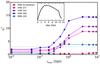 |
Fig. 10 Variations in the χ2 as a function of τtrunc for the five galaxies presented in Fig. 2. The horizontal dotted line shows a χ2 of 3 below which fits are usually considered as good. The insert panel shows the shape of the SFH considered in this test. |
In Sect. 5.3, we correct the SFR of the Hi-deficient galaxies to show that they were once on the main sequence relation. However, even unperturbed objects have rSFR that is not exactly equal to one but scattered in the 0.7−1 range. These high values of rSFR translate into a slow decrease in their SFR. We did not correct the SFR of these sources as we know from their Hi-deficiency that they did not undergo a rapid decrease in their star formation activity. As we discuss in Sect. 5.2, the Hi−def parameter is not available for a lot of sources and catalogs. Thus some other criteria and associated methodology should be applied in order to identify systems that underwent a rapid decrease in their star formation activity and estimate their SFR prior to quenching. As shown in Fig. 8, the mean value of rSFR at Hi−def = 0.4, the typical value separating the gas-rich from the Hi-deficient galaxies is 0.3. Thus one possibility is to consider them as quenched sources with rSFR ≤ 0.3. Another possibility is to decide an arbitrary cut in the ratio between the χ2 obtained for the delayed and truncated SFH to estimate which of the two SFH models the SED better.
The HRS galaxies benefit from a wealth of photometric data from UV-to-submm. However, at higher redshifts, IR observations are not always available, and the photometric coverage of these sources often stops with WISE or Spitzer/MIPS 22−24 μm data or even at Spitzer/IRAC wavelengths. We show in Fig. 11 the relation between the rSFR values obtained with a full photometric coverage and the values obtained stopping at 22 μm and then at 8 μm rest frame. There is a weak underestimate of the parameter in the absence of IR data, as well as an increase in the dispersion. However, the differences are still smaller than the error bars. We notice that the estimates of low rSFR (<0.2) values are consistent with the one obtained with the full coverage. The dispersion is, however, higher for higher rSFR values. We conclude from this test that the results of this work hold for source for which the IR domain is not well covered.
 |
Fig. 11 Impact of the photometric coverage on the derivation of the rSFR parameter. Pink points show the relation between the values obtained when the photometric coverage stops at 22 μm and the values obtained from a full coverage. The purple points show the relation when the photometric coverage stops at 8 μm. Mean error bars are shown for both subsets. |
We tested our method on local galaxies with a relatively low dust attenuation. However, in the redshift range z = 1−3, UV galaxy emission is deeply obscured by dust absorption. To evaluate the ability of our SED fitting method to identify star formation quenching at these redshifts, we followed the method presented in Sect. 4.3 to build a mock catalog of z = 2 galaxies. We assumed AFUV = 4 mag as a mean attenuation at redshift 2, determined by Buat et al. (2015). The results of the mock analysis are presented in Fig. 12. As for z = 0 galaxies, the agetrunc parameter is not constrained, regardless of the value of τmain. However, with small variations around the one-to-one relationship, the rSFR parameter is relatively well recovered. The main difference compared to the mock analysis of z = 0 sources is the good constraint on rSFR when τmain = 3 Gyr. The results of this test imply that the method proposed in this work can be applied to high redshift galaxies.
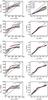 |
Fig. 12 Results of the z = 2 mock catalog analysis for the two parameters agetrunc and rSFR. The five left panels present the constraint on agetrunc for five different τmain (1, 3, 5, 7, and 10 Gyr). The colored lines corresponds to different values of rSFR. The five righthand panels display the constraint on rSFR for the same five values of τmain (1, 3, 5, 7, and 10 Gyr), the colored lines corresponding to different agetrunc. On each panel, the black solid line is the one-to-one relationship. |
In this study, we discuss ram pressure stripping as an example of rapid quenching because we have a sample of local galaxies with sufficient photometric coverage and ancillary data to test the effect of this mechanism on the SED of galaxies. However, even though we focused on one particular mechanism, the results of this work suggest than broad-band SED fitting is a powerful tool for identifying peculiar SFH of galaxies, such as rapid drop in the star formation activity. Indeed, SFH modelis of a recent burst in the star formation activity are widely used in the literature (e.g., Papovich et al. 2001; Borch et al. 2006; Gawiser et al. 2007; Lee et al. 2009; Buat et al. 2014), however we show in this work that a rapid decrease can also be identified.
7. Conclusions
We defined a truncated delayed SFH to model the SEDs of galaxies that underwent a rapid quenching of their star formation activity. Using the CIGALE SED fitting code, we showed that the ratio between the instantaneous SFR and the SFR just before the truncation of the SFH is well constrained as long as UV rest frame data are available.
This SED fitting procedure is applied to the Herschel Reference Survey (HRS) since it contains both isolated galaxies and sources lying in the dense environment of the Virgo cluster. These objects are Hi-deficient owing to ram pressure occurring in the cluster. We showed that the truncated delayed SFH manages to reproduce their UV-to-NIR SED, while the usual SFH assumptions fail. An anti-correlation is found between rSFR and Hi−def, which is the parameter quantifying the gas deficiency of the Virgo galaxies with a Spearman correlation coefficient of −0.67, implying that SED fitting can be used to provide a tentative estimate of the gas deficiency of galaxies for which Hi observations are not available. The HRS galaxies are placed on the SFR-M∗ diagram showing that the Hi-deficient sources lie in the quiescent region in agreement with what was found in previous studies. Using the rSFR parameter, we derive the SFR of these sources before quenching and show that they were initially on the galaxy main sequence relation.
We discussed the assumption made on an instantaneous break in the SFH and showed that it holds for quenching mechanisms affecting the star formation activity in less than 200−500 Myr. The estimate of rSFR in the absence of IR data is consistent with what has been obtained with a full photometric coverage within the error bars. Furthermore, the truncated SFH proposed in this work can also be used for deeply obscured (AFUV ≈ 4 mag) high redshift sources. SED fitting is thus a powerful tool for identifying galaxies that underwent a rapid star formation quenching and can provide a tentative estimate of their gas deficiency.
With respect to the original sample given in Boselli et al. (2010), the galaxy HRS 228 is removed from the complete sample because its updated redshift on NED indicates it is a background object.
The code is publicly available at: http://cigale.lam.fr/
Acknowledgments
We thank the referee for comments that helped improve this paper. L.C. warmly thanks M. Boquien, Y. Roehlly, and D. Burgarella for developing the new version of CIGALE on which the present work relies and L. Cortese for useful comments. L.C. benefited from the thales project 383549 that is jointly funded by the European Union and the Greek Government in the framework of the program “Education and lifelong learning”. The research leading to these results has received funding from the European Union Seventh Framework Program (FP7/2007-2013) under grant agreement no. 312725.
References
- Baldry, I. K., Glazebrook, K., Brinkmann, J., et al. 2004, ApJ, 600, 681 [NASA ADS] [CrossRef] [Google Scholar]
- Baldry, I. K., Balogh, M. L., Bower, R. G., et al. 2006, MNRAS, 373, 469 [NASA ADS] [CrossRef] [Google Scholar]
- Bekki, K. 2009, MNRAS, 399, 2221 [NASA ADS] [CrossRef] [Google Scholar]
- Bell, E. F., Wolf, C., Meisenheimer, K., et al. 2004, ApJ, 608, 752 [NASA ADS] [CrossRef] [Google Scholar]
- Bendo, G. J., Galliano, F., & Madden, S. C. 2012, MNRAS, 423, 197 [NASA ADS] [CrossRef] [Google Scholar]
- Boquien, M., Buat, V., & Perret, V. 2014, A&A, 571, A72 [NASA ADS] [CrossRef] [EDP Sciences] [Google Scholar]
- Borch, A., Meisenheimer, K., Bell, E. F., et al. 2006, A&A, 453, 869 [NASA ADS] [CrossRef] [EDP Sciences] [Google Scholar]
- Boselli, A., & Gavazzi, G. 2009, A&A, 508, 201 [NASA ADS] [CrossRef] [EDP Sciences] [Google Scholar]
- Boselli, A., & Gavazzi, G. 2014, A&ARv, 22, 74 [NASA ADS] [CrossRef] [Google Scholar]
- Boselli, A., Gavazzi, G., Donas, J., & Scodeggio, M. 2001, AJ, 121, 753 [NASA ADS] [CrossRef] [Google Scholar]
- Boselli, A., Boissier, S., Cortese, L., et al. 2006, ApJ, 651, 811 [NASA ADS] [CrossRef] [Google Scholar]
- Boselli, A., Boissier, S., Cortese, L., & Gavazzi, G. 2008, ApJ, 674, 742 [NASA ADS] [CrossRef] [Google Scholar]
- Boselli, A., Eales, S., Cortese, L., et al. 2010, PASP, 122, 261 [NASA ADS] [CrossRef] [Google Scholar]
- Boselli, A., Ciesla, L., Cortese, L., et al. 2012, A&A, 540, A54 [NASA ADS] [CrossRef] [EDP Sciences] [Google Scholar]
- Boselli, A., Hughes, T. M., Cortese, L., Gavazzi, G., & Buat, V. 2013, A&A, 550, A114 [NASA ADS] [CrossRef] [EDP Sciences] [Google Scholar]
- Boselli, A., Cortese, L., & Boquien, M. 2014a, A&A, 564, A65 [NASA ADS] [CrossRef] [EDP Sciences] [Google Scholar]
- Boselli, A., Cortese, L., Boquien, M., et al. 2014b, A&A, 564, A67 [NASA ADS] [CrossRef] [EDP Sciences] [Google Scholar]
- Boselli, A., Fossati, M., Gavazzi, G., et al. 2015, A&A, 579, A102 [NASA ADS] [CrossRef] [EDP Sciences] [Google Scholar]
- Brown, T., Catinella, B., Cortese, L., et al. 2015, MNRAS, 452, 2479 [NASA ADS] [CrossRef] [Google Scholar]
- Bruzual, G., & Charlot, S. 2003, MNRAS, 344, 1000 [NASA ADS] [CrossRef] [Google Scholar]
- Buat, V., Heinis, S., Boquien, M., et al. 2014, A&A, 561, A39 [NASA ADS] [CrossRef] [EDP Sciences] [Google Scholar]
- Buat, V., Oi, N., Heinis, S., et al. 2015, A&A, 577, A141 [NASA ADS] [CrossRef] [EDP Sciences] [Google Scholar]
- Calzetti, D., Armus, L., Bohlin, R. C., et al. 2000, ApJ, 533, 682 [NASA ADS] [CrossRef] [Google Scholar]
- Casey, C. M. 2012, MNRAS, 425, 3094 [Google Scholar]
- Catinella, B., Schiminovich, D., Cortese, L., et al. 2013, MNRAS, 436, 34 [NASA ADS] [CrossRef] [Google Scholar]
- Ciesla, L., Boselli, A., Smith, M. W. L., et al. 2012, A&A, 543, A161 [NASA ADS] [CrossRef] [EDP Sciences] [Google Scholar]
- Ciesla, L., Boquien, M., Boselli, A., et al. 2014, A&A, 565, A128 [Google Scholar]
- Ciesla, L., Charmandaris, V., Georgakakis, A., et al. 2015, A&A, 576, A10 [NASA ADS] [CrossRef] [EDP Sciences] [Google Scholar]
- Cortese, L., & Hughes, T. M. 2009, MNRAS, 400, 1225 [NASA ADS] [CrossRef] [Google Scholar]
- Cortese, L., Davies, J. I., Pohlen, M., et al. 2010, A&A, 518, L49 [NASA ADS] [CrossRef] [EDP Sciences] [Google Scholar]
- Cortese, L., Catinella, B., Boissier, S., Boselli, A., & Heinis, S. 2011, MNRAS, 415, 1797 [NASA ADS] [CrossRef] [Google Scholar]
- Cortese, L., Boissier, S., Boselli, A., et al. 2012a, A&A, 544, A101 [NASA ADS] [CrossRef] [EDP Sciences] [Google Scholar]
- Cortese, L., Ciesla, L., Boselli, A., et al. 2012b, A&A, 540, A52 [NASA ADS] [CrossRef] [EDP Sciences] [Google Scholar]
- Cortese, L., Fritz, J., Bianchi, S., et al. 2014, MNRAS, 440, 942 [NASA ADS] [CrossRef] [Google Scholar]
- Crowl, H. H., & Kenney, J. D. P. 2008, AJ, 136, 1623 [NASA ADS] [CrossRef] [Google Scholar]
- Dale, D. A., Helou, G., Magdis, G. E., et al. 2014, ApJ, 784, 83 [NASA ADS] [CrossRef] [Google Scholar]
- Draine, B. T., & Li, A. 2007, ApJ, 657, 810 [NASA ADS] [CrossRef] [Google Scholar]
- Dressler, A. 1980, ApJ, 236, 351 [NASA ADS] [CrossRef] [Google Scholar]
- Elbaz, D., Daddi, E., Le Borgne, D., et al. 2007, A&A, 468, 33 [NASA ADS] [CrossRef] [EDP Sciences] [Google Scholar]
- Elbaz, D., Dickinson, M., Hwang, H. S., et al. 2011, A&A, 533, A119 [NASA ADS] [CrossRef] [EDP Sciences] [Google Scholar]
- Fabello, S., Catinella, B., Giovanelli, R., et al. 2011, MNRAS, 411, 993 [NASA ADS] [CrossRef] [Google Scholar]
- Fritz, J., Franceschini, A., & Hatziminaoglou, E. 2006, MNRAS, 366, 767 [Google Scholar]
- Fumagalli, M., Gavazzi, G., Scaramella, R., & Franzetti, P. 2011, A&A, 528, A46 [NASA ADS] [CrossRef] [EDP Sciences] [Google Scholar]
- Gavazzi, G., Pierini, D., & Boselli, A. 1996, A&A, 312, 397 [NASA ADS] [Google Scholar]
- Gavazzi, G., Boselli, A., van Driel, W., & O’Neil, K. 2005, A&A, 429, 439 [NASA ADS] [CrossRef] [EDP Sciences] [Google Scholar]
- Gawiser, E., Francke, H., Lai, K., et al. 2007, ApJ, 671, 278 [NASA ADS] [CrossRef] [Google Scholar]
- Gil de Paz, A., Boissier, S., Madore, B. F., et al. 2007, ApJS, 173, 185 [NASA ADS] [CrossRef] [Google Scholar]
- Giovannoli, E., Buat, V., Noll, S., Burgarella, D., & Magnelli, B. 2011, A&A, 525, A150 [NASA ADS] [CrossRef] [EDP Sciences] [Google Scholar]
- Gladders, M. D., Oemler, A., Dressler, A., et al. 2013, ApJ, 770, 64 [NASA ADS] [CrossRef] [Google Scholar]
- Gunn, J. E., & Gott, III, J. R. 1972, ApJ, 176, 1 [NASA ADS] [CrossRef] [Google Scholar]
- Haines, C. P., Pereira, M. J., Smith, G. P., et al. 2013, ApJ, 775, 126 [NASA ADS] [CrossRef] [EDP Sciences] [Google Scholar]
- Haines, C. P., Pereira, M. J., Smith, G. P., et al. 2015, ApJ, 806, 101 [NASA ADS] [CrossRef] [Google Scholar]
- Haynes, M. P., Magri, C. A., & Giovanelli, R. 1984, in BAAS, 16, 882 [Google Scholar]
- Hughes, T. M., & Cortese, L. 2009, MNRAS, 396, L41 [NASA ADS] [CrossRef] [Google Scholar]
- Ilbert, O., McCracken, H. J., Le Fèvre, O., et al. 2013, A&A, 556, A55 [NASA ADS] [CrossRef] [EDP Sciences] [Google Scholar]
- Kronberger, T., Kapferer, W., Ferrari, C., Unterguggenberger, S., & Schindler, S. 2008, A&A, 481, 337 [NASA ADS] [CrossRef] [EDP Sciences] [Google Scholar]
- Lee, S.-K., Idzi, R., Ferguson, H. C., et al. 2009, ApJS, 184, 100 [NASA ADS] [CrossRef] [Google Scholar]
- Maraston, C. 2005, MNRAS, 362, 799 [NASA ADS] [CrossRef] [Google Scholar]
- Maraston, C., Pforr, J., Renzini, A., et al. 2010, MNRAS, 407, 830 [NASA ADS] [CrossRef] [Google Scholar]
- McGee, S. L., Balogh, M. L., Bower, R. G., Font, A. S., & McCarthy, I. G. 2009, MNRAS, 400, 937 [NASA ADS] [CrossRef] [Google Scholar]
- Mori, M., & Burkert, A. 2000, ApJ, 538, 559 [NASA ADS] [CrossRef] [Google Scholar]
- Noeske, K. G., Weiner, B. J., Faber, S. M., et al. 2007, ApJ, 660, L43 [Google Scholar]
- Noll, S., Burgarella, D., Giovannoli, E., et al. 2009, A&A, 507, 1793 [NASA ADS] [CrossRef] [EDP Sciences] [Google Scholar]
- Papovich, C., Dickinson, M., & Ferguson, H. C. 2001, ApJ, 559, 620 [NASA ADS] [CrossRef] [Google Scholar]
- Pappalardo, C., Lançon, A., Vollmer, B., et al. 2010, A&A, 514, A33 [NASA ADS] [CrossRef] [EDP Sciences] [Google Scholar]
- Peng, Y.-j.,Lilly, S. J., Kovač, K., et al. 2010, ApJ, 721, 193 [NASA ADS] [CrossRef] [Google Scholar]
- Pforr, J., Maraston, C., & Tonini, C. 2012, MNRAS, 422, 3285 [NASA ADS] [CrossRef] [Google Scholar]
- Querejeta, M., Meidt, S. E., Schinnerer, E., et al. 2015, ApJS, 219, 5 [NASA ADS] [CrossRef] [Google Scholar]
- Quilis, V., Moore, B., & Bower, R. 2000, Science, 288, 1617 [NASA ADS] [CrossRef] [PubMed] [Google Scholar]
- Roediger, E., & Brüggen, M. 2007, MNRAS, 380, 1399 [NASA ADS] [CrossRef] [Google Scholar]
- Roehlly, Y., Burgarella, D., Buat, V., et al. 2014, in Astronomical Data Analysis Software and Systems XXIII, eds. N. Manset, & P. Forshay, ASP Conf. Ser., 485, 347 [Google Scholar]
- Salim, S., Charlot, S., Rich, R. M., et al. 2005, ApJ, 619, L39 [Google Scholar]
- Salpeter, E. E. 1955, ApJ, 121, 161 [Google Scholar]
- Schaerer, D., de Barros, S., & Sklias, P. 2013, A&A, 549, A4 [NASA ADS] [CrossRef] [EDP Sciences] [Google Scholar]
- Sparre, M., Hayward, C. C., Springel, V., et al. 2015, MNRAS, 447, 3548 [Google Scholar]
- Speagle, J. S., Steinhardt, C. L., Capak, P. L., & Silverman, J. D. 2014, ApJS, 214, 15 [NASA ADS] [CrossRef] [Google Scholar]
- Strateva, I., Ivezić, Ž., Knapp, G. R., et al. 2001, AJ, 122, 1861 [Google Scholar]
- Tonnesen, S., & Bryan, G. L. 2009, ApJ, 694, 789 [NASA ADS] [CrossRef] [Google Scholar]
- Vollmer, B. 2009, A&A, 502, 427 [NASA ADS] [CrossRef] [EDP Sciences] [Google Scholar]
- Vollmer, B., Balkowski, C., Cayatte, V., van Driel, W., & Huchtmeier, W. 2004, A&A, 419, 35 [NASA ADS] [CrossRef] [EDP Sciences] [Google Scholar]
- Vollmer, B., Braine, J., Pappalardo, C., & Hily-Blant, P. 2008, A&A, 491, 455 [NASA ADS] [CrossRef] [EDP Sciences] [Google Scholar]
- Vollmer, B., Soida, M., Braine, J., et al. 2012, A&A, 537, A143 [NASA ADS] [CrossRef] [EDP Sciences] [Google Scholar]
- Weinmann, S. M., Kauffmann, G., von der Linden, A., & De Lucia, G. 2010, MNRAS, 406, 2249 [NASA ADS] [CrossRef] [Google Scholar]
- Weisz, D. R., Johnson, B. D., Johnson, L. C., et al. 2012, ApJ, 744, 44 [NASA ADS] [CrossRef] [Google Scholar]
Appendix A: Results from SED fitting: agetrunc as a free parameter
The distribution of the χ2, M∗, SFR, rSFR, τmain, and agetrunc obtained from the SED fitting, with agetrunc left as a free parameter, are presented in Fig. A.1 for both normal and Hi-deficient galaxies. The χ2 distribution for both the normal and the Hi-deficient samples is similar with a mean value of 1.43 and 1.08, respectively. The distributions of the stellar mass of both subsamples are similar, peaking at the same value as the results from the run fixing agetrunc. The distribution of star formation rates of the Hi-deficient clearly shows that most of these galaxies have a very low, almost zero. The distribution of the rSFR parameter shows two different behaviors for normal and deficient galaxies. The Hi-deficient subsample distribution shows lower values with 42 sources with rSFR< 0.15 out of 92 deficients galaxies. The rSFR distribution of normal galaxies is flat and shifted toward higher values, although not as close to 1 as one would expect. The distribution of agetrunc is very similar for both samples with about the same mean value (321 Myr for the normal galaxies and 350 Myr for the deficient sample) and same distribution. This behavior reinforces our conclusion about the poor constraint on this parameter. Finally, the distribution of τmain shows that most of the sources have τmain ≥ 5 Gyr in this configuration, too.
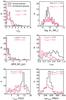 |
Fig. A.1 Distribution of the output parameters obtained from the SED fitting procedure with CIGALE. The results for the normal galaxy sample are shown in gray, while the results for the Hi-deficient sample are shown in red. |
Appendix B: NUV-r versus Hi–def relation for the HRS galaxies
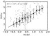 |
Fig. B.1 NUV-r color as a function of Hi−def for the HRS galaxies studied in this work. Black triangles show the median values in 0.2 Hi−def bins, and the error bars represent the standard deviation in each bin. The Spearman correlation coefficient and the results of the best linear fit are indicated. |
It is established now that the NUV-r color is a good tracer of the gas content of galaxies (e.g., Cortese et al. 2011; Fabello et al. 2011; Catinella et al. 2013; Brown et al. 2015), so we show in Fig. B.1 the NUV-r versus Hi−def relations for the galaxies studied in this work. Using the same bins as in Fig. 8, we obtained a best linear fit of  (B.1)associated with a Spearman correlation coefficient of 0.61.
All Tables
Mean obtained using the three SFHs mentioned in this work and for three bins of Hi−def.
All Figures
|
Fig. 1 Illustration of the truncated delayed SFH implemented in CIGALE. The purple dashed line represents a normal delayed SFH with τmain = 5 Gyr, without truncation. The red solid line is the truncated delayed SFH. |
| In the text | |
|
Fig. 2 Left column: examples of best fits obtained with CIGALE for one normal and four Hi-deficient HRS galaxies using three different SFHs assumptions: a delayed SFH (navy blue), a 2-exponentially decreasing SFH (cyan), and a truncated delayed SFH (red). Right column: for each galaxy, the output best fit SFH obtained for the three different assumptions made. |
| In the text | |
|
Fig. 3 Impact of the two parameters, agetrunc (upper panel) and rSFR (lower panel), on the SED considering a τmain of 10 Gyr. SEDs are color-coded according to the value of the free parameter. For clarity, we only show models with rSFR lower than 0.45 in this plot. At the bottom of each panel, we show the filters of GALEX (red), SDSS, and 2MASS. |
| In the text | |
|
Fig. 4 Constraints on τmain as a result of the mock catalog analysis of the truncated SFH parameters. The dispersion of the output values are shown in blue, the mean and 64th percentile for each input values in black. The black solid line is the one-to-one relationship. The right panel shows the distribution of the points for each input value of τmain. |
| In the text | |
|
Fig. 5 Results of the mock catalog analysis for the two parameters agetrunc and rSFR. The five lefthand panels present the constraint on agetrunc for five different τmain (1, 3, 5, 7, and 10 Gyr). The colored lines correspond to different values of rSFR. The five right panels display the constraint on rSFR for the same five values of τmain (1, 3, 5, 7, and 10 Gyr), and the colored lines correspond to different agetrunc. In each panel, the black solid line is the one-to-one relationship. |
| In the text | |
|
Fig. 6 Comparison between the stellar masses (top panel) and SFR (bottom panel) obtained using the truncated and normally delayed SFH. Normal galaxies are shown in gray, whereas Hi-deficient and highly deficient galaxies (with Hi−def≥ 1) are shown in red and yellow, respectively. The black solid lines represent the one-to-one relationship. |
| In the text | |
|
Fig. 7 Distribution of the output parameters obtained from the SED fitting procedure with CIGALE. The results for the normal galaxy sample are shown in gray while the results for the Hi-deficient sample are shown in red. |
| In the text | |
|
Fig. 8 Relation between rSFR and the Hi deficiency. Data points are color-coded according to the value of τmain obtained from the fit. The mean errors bars for each subsample are provided with the red star for the normal galaxy sample and with the red filled circle for the deficient galaxies. The Spearman correlation coefficient ρ of the relation is indicated. Black triangles are the median values in bins of ΔHi−def= 0.2, and the error bars are the standard deviation of the points in each bins. The black filled line is the best linear fit to the data. The black dotted line indicates the adopted threshold used to separate normal from deficient galaxies. |
| In the text | |
|
Fig. 9 Relation between the SFR and M∗ of the HRS subsamples. Black stars are the normal galaxies, filled circles are the Hi-deficient galaxies color-coded according to the Hi−def parameter. Yellow crosses point out the sources for which rSFR = 0. Main sequence relations found at z = 0 are shown in dashed lines: in blue the one from Ciesla et al. (2014), in red the relation of Peng et al. (2010), and the relation derived in this work is the black solid line. Top panel: observed relation obtained with CIGALE. Bottom panel: estimated positions of the Hi-deficient galaxies before interaction with the environment obtained after correcting their instantaneous SFR with the rSFR parameter. |
| In the text | |
|
Fig. 10 Variations in the χ2 as a function of τtrunc for the five galaxies presented in Fig. 2. The horizontal dotted line shows a χ2 of 3 below which fits are usually considered as good. The insert panel shows the shape of the SFH considered in this test. |
| In the text | |
|
Fig. 11 Impact of the photometric coverage on the derivation of the rSFR parameter. Pink points show the relation between the values obtained when the photometric coverage stops at 22 μm and the values obtained from a full coverage. The purple points show the relation when the photometric coverage stops at 8 μm. Mean error bars are shown for both subsets. |
| In the text | |
|
Fig. 12 Results of the z = 2 mock catalog analysis for the two parameters agetrunc and rSFR. The five left panels present the constraint on agetrunc for five different τmain (1, 3, 5, 7, and 10 Gyr). The colored lines corresponds to different values of rSFR. The five righthand panels display the constraint on rSFR for the same five values of τmain (1, 3, 5, 7, and 10 Gyr), the colored lines corresponding to different agetrunc. On each panel, the black solid line is the one-to-one relationship. |
| In the text | |
|
Fig. A.1 Distribution of the output parameters obtained from the SED fitting procedure with CIGALE. The results for the normal galaxy sample are shown in gray, while the results for the Hi-deficient sample are shown in red. |
| In the text | |
|
Fig. B.1 NUV-r color as a function of Hi−def for the HRS galaxies studied in this work. Black triangles show the median values in 0.2 Hi−def bins, and the error bars represent the standard deviation in each bin. The Spearman correlation coefficient and the results of the best linear fit are indicated. |
| In the text | |
Current usage metrics show cumulative count of Article Views (full-text article views including HTML views, PDF and ePub downloads, according to the available data) and Abstracts Views on Vision4Press platform.
Data correspond to usage on the plateform after 2015. The current usage metrics is available 48-96 hours after online publication and is updated daily on week days.
Initial download of the metrics may take a while.