© G. Aufort et al. 2020

1. Introduction

The tight relation linking the star formation rate (SFR) and stellar mass of star-forming galaxies, the so-called main sequence (MS), opened a new window in our understanding of galaxy evolution (Elbaz et al. 2007; Noeske et al. 2007). It implies that the majority of galaxies are likely to form the bulk of their stars through steady-state processes rather than violent episodes of star formation. However, this relation has a scatter of ∼0.3 dex (Schreiber et al. 2015) that is found to be relatively constant at all masses and over cosmic time (Guo et al. 2013; Ilbert et al. 2015; Schreiber et al. 2015). One possible explanation of this scatter could be its artificial creation by the accumulation of errors in the extraction of photometric measurements and/or in the determination of the SFR and stellar mass in relation with model uncertainties. However, several studies have found a coherent variation in physical galaxy properties such as the gas fraction (Magdis et al. 2012), Sérsic index and effective radius (Wuyts et al. 2011), and U − V color (e.g., Salmi et al. 2012), suggesting that the scatter is more strongly related to the physics than to measurement and model uncertainties. Furthermore, oscillations in SFR resulting from a varying infall rate and compaction of star formation have been proposed to explain the MS scatter (Sargent et al. 2014; Scoville et al. 2016; Tacchella et al. 2016) and en even be suggested by some simulations (e.g., Dekel & Burkert 2014).

To decipher whether the scatter is indeed due to variations in star formation history (SFH), we must be able to place a constraint on the recent SFH of galaxies to reconstruct their path along the MS. This information is embedded in the spectral energy distribution (SED) of galaxies. However, recovering it through SED modeling is complex and subject to many uncertainties and degeneracies. Galaxies are indeed expected to exhibit complex SFHs, with short-term fluctuations. This requires sophisticated SFH parametrizations to model them (e.g., Lee et al. 2010; Pacifici et al. 2013, 2016; Behroozi et al. 2013; Leja et al. 2019). The implementation of these models is complex, and large libraries are needed to model all galaxy properties. Numerous studies have instead used simple analytical forms to model galaxies SFH (e.g., Papovich et al. 2001; Maraston et al. 2010; Pforr et al. 2012; Gladders et al. 2013; Simha et al. 2014; Buat et al. 2014; Boquien et al. 2014; Ciesla et al. 2015, 2016, 2017; Abramson et al. 2016). However, SFH parameters are known to be difficult to constrain from broadband SED modeling (e.g., Maraston et al. 2010; Pforr et al. 2012; Buat et al. 2014; Ciesla et al. 2015, 2017; Carnall et al. 2019).

Ciesla et al. (2016) and Boselli et al. (2016) have shown in a sample of well-known local galaxies benefiting from a wealth of ancillary data that a drastic and recent decrease in star formation activity of galaxies can be probed as long as a good UV to near-IR (NIR) rest frame coverage is available. They showed that the intensity in the variation of the star formation (SF) activity can be relatively well constrained from broadband SED fitting. Spectroscopy is required, however, to bring information on the time when the change in star formation activity occurred (Boselli et al. 2016). These studies were made on well-known sources of the Virgo cluster, for which the quenching mechanism (ram pressure stripping) is known and HI observations allow a direct verification of the SED modeling results. To go a step further, Ciesla et al. (2018) have blindly applied the method on the GOODS-South sample to identify sources that underwent a recent and drastic decrease in their SF activity. They compared the quality of the results from SED fitting using two different SFHs and obtained a sample of galaxies where a modeled recent and strong decrease in SFR produced significantly better fits of the broadband photometry. In this work, we improve the method of Ciesla et al. (2018) by gaining in power by applying a custom statistical method to a subsample of COSMOS galaxies to perform the SFH choice: the approximate Bayesian computation (ABC, see, e.g., Marin et al. 2012; Sisson et al. 2018). Based on the observed SED of a galaxy, we wish to choose the most appropriate SFH in a finite set. The main idea behind ABC is to rely on many simulated SEDs generated from all the SFHs in competition using parameters drawn from the prior.

The paper is organized as follows: Sect. 2 describes the astrophysical problem and presents the sample. In Sect. 3 we present the statistical approach as well as the results obtained from a catalog of simulated SEDs of COSMOS-like galaxies. In Sect. 4 we compare the results of this new approach with more traditional SED modeling methods, and apply it to real COSMOS galaxies in Sect. 5. Our results are discussed in Sect. 6.

2. Constraining the recent star formation history of galaxies using broadband photometry

2.1. Building upon the method of Ciesla et al. (2018)

The main purpose of the study presented in Ciesla et al. (2018) was to probe variations in SFH that occurred on very short timescales, that is, within some hundred million years. Large-number statistics was needed to be able to catch galaxies at the moment when these variations occurred. The authors aimed at identifying galaxies that recently underwent a rapid (< 500 Myr) and drastic downfall in SFR (more than 80%) from broadband SED modeling because large photometric samples can provide the statistics needed to pinpoint these objects.

To perform their study, they took advantage of the versatility of the SED modeling code CIGALE¹ (Boquien et al. 2019). CIGALE is a SED modeling software package that has two functions: a modeling function to create SEDs from a set of given parameters, and an SED fitting function to derive the physical properties of galaxies from observations. Galaxy SEDs are computed from UV-to-radio taking into account the balance between the energy absorbed by dust in the UV-NIR and remitted in IR. To build the SEDs, CIGALE uses a combination of modules including the SFH assumption, which may be analytical, stochastic, or outputs from simulations (e.g., Boquien et al. 2014; Ciesla et al. 2015, 2017), the stellar emission from stellar population models (Bruzual & Charlot 2003; Maraston 2005), the nebular lines, and the attenuation by dust (e.g., Calzetti et al. 2000; Charlot & Fall 2000).

Ciesla et al. (2018) compared the results of SED fitting in a sample of GOODS-South galaxies using two different SFHs: one normal delayed-τ SFH, and one flexible SFH that modeled a truncation of the SFH. The normal delayed-τ SFH is given by the equation

$$\begin{array}{c}\hfill \mathrm{SFR}(t)\propto t\times exp(-t/{\tau }_{\mathrm{main}}),\end{array}$$(1)

where SFR is the star formation rate, t is the time, and τ_main is the e-folding time. Examples of delayed-τ SFHs are shown in Fig. 1 for different values of τ_main. The flexible SFH is an extension of the delayed-τ model,

$$\begin{array}{c}\hfill \mathrm{SFR}(t)\propto \{\begin{array}{cc}t\times exp(-t/{\tau }_{\mathrm{main}}),\hfill & \mathrm{when}t\le t_{\mathrm{flex}}\hfill \\ r_{\mathrm{SFR}}\times \mathrm{SFR}(t=t_{\mathrm{flex}}),\hfill & \mathrm{when}t>t_{\mathrm{flex}}\hfill \end{array},\end{array}$$(2)

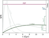Fig. 1. Examples of delayed-τ SFHs considered in this work (star formation rate as a function of cosmic time). Different SFHs using τmain = 0.5, 1, 5, and 10 Gyr are shown to illustrate the effect of this parameter (light green and dark green solid lines). An example of a delayed-τ SFH with flexibility is shown in solid dark green, with the flexibility as green dashed lines for (ageflex = 1 Gyr and rSFR = 0.3) and (ageflex = 0.5 Gyr and rSFR = 7).

where t_flex is the time at which the star formation is instantaneously affected, and r_SFR is the ratio between SFR(t >  t_flex) and SFR(t = t_flex),

$$\begin{array}{c}\hfill r_{\mathrm{SFR}}=\frac{\mathrm{SFR}(t>t_{\mathrm{flex}})}{\mathrm{SFR}(t_{\mathrm{flex}})}·\end{array}$$(3)

A representation of flexible SFHs is also shown in Fig. 1. The normal delayed-τ SFH is at first order a particular case of the flexible SFH for which r_SFR = 1.

To distinguish between the two models, Ciesla et al. (2018) estimated the Bayesian information criterion (BIC, see Sect. 3.2) that is linked to the two models and placed conservative limits on the difference between the two BICs to select the best-suited model. They showed that a handful of sources were better fit using the flexible SFH, which assumes a recent instantaneous break in the SFH, compared to the more commonly used delayed-τ SFH. They discussed that these galaxies have indeed physical properties that are different from the main population and characteristic of sources in transition.

The limited number of sources identified in the study of Ciesla et al. (2018; 102 out of 6680) was due to their choice to be conservative in their approach and find a clean sample of sources that underwent a rapid quenching of star formation. They imposed that the instantaneous decrease of SFR was more than 80% and that the BIC difference was larger than 10. These criteria prevent a complete study of rapid variations in the SFH of galaxies because many of them would be missed. Furthermore, only decreases in SFR were considered and not the opposite, that is, star formation bursts. Finally, their method is time consuming because the CIGALE code has to be run twice, once per SFH model considered, to perform the analysis. To go beyond these drawbacks and improve the method of Ciesla et al. (2018), we consider in the present pilot study a statistical approach, the ABC, combined with a classification algorithm to improve the accuracy and efficiency of their method.

2.2. Sample

In this pilot work, we use the wealth of data available on the COSMOS field. The choice of this field is driven by the good spectral coverage of the data and the large statistics of sources.

We drew a sample from the COSMOS catalog of Laigle et al. (2016). A first cut was made to restrict ourselves to galaxies with a stellar mass (Laigle et al. 2016) higher than 10^8.5 M_⊙. Then we restricted the sample to a relatively narrow redshift range to minimize its effect on the SED and focus our method on the SFH effect on the SED. We therefore selected galaxies with redshifts between 0.5 and 1, which ensures sufficient statistics in our sample. We used the broadbands of the COSMOS catalog as listed in Table 1. For galaxies with redshifts between 0.5 and 1, Spitzer/IRAC3 probes the 2.9–3.9 μm wavelength range rest frame and Spitzer/IRAC4 probes the 4–5.3 μm range rest frame. These wavelength ranges correspond to the transition between stellar and dust emission. To keep this pilot study simple, we only considered the UV-to-NIR part of the spectrum, which is not affected by dust emission.

One aspect of the ABC method that is still to be developed is handling missing data. In our astrophysical application, we identified several types of missing data. First there is the effect of redshifting, that is, the fact that a galaxy is undetected at wavelengths shorter than the Lyman break at its redshift. Here, the absence of detection provides information on the galaxy coded in its SED. Another type of missing data is linked to the definition of the photometric surveys: the spatial coverage is not exactly the same in every band, and the different sensitivity limits yield undetected galaxies because their fluxes are afaint. To keep the statistical problem simple in this pilot study, we removed galaxies that were not detected in all bands. This strong choice is motivated by the fact that the ABC method that we use in this pilot study has not been tested and calibrated in the case of missing data such as extragalactic field surveys can produce. The effect of missing data on this method would require much work of statistical research, which is beyond the scope of this paper.

As an additional constraint, we selected galaxies with a signal-to-noise ratio (S/N) equal or greater than 10. However, given the importance of the near-UV (NUV) band (Ciesla et al. 2016, 2018) and the faintness of the fluxes compared to the other bands, we relaxed our criteria to an S/N of 5 for this band. The first motivation for this cut was again to keep our pilot study simple, but we show in Appendix A that this S/N cut is relevant. In the following, we consider a final sample composed of 12 380 galaxies for which the stellar mass distribution as a function of redshift is shown in Fig. 2 (top panel) and the distribution of the rejected sources in the bottom panel of the same figure.

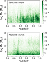Fig. 2. Stellar mass from Laigle et al. (2016) as a function of redshift for the final sample (top panel) and for the rejected galaxies following our criteria (bottom panel).

The stellar mass distribution, from Laigle et al. (2016), of the final sample is shown in Fig. 3. As a sanity check, we verified that above 10^9.5 M_⊙, the stellar mass, star formation rate, and specific star formation rate distributions are similar. Our selection criteria mostly affect low-mass galaxies, which is expected because we made S/N cuts.

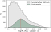Fig. 3. Distribution of stellar mass for the sample before the S/N cut (gray) and the final sample (green). The red dotted line indicates the limit above which our final sample is considered complete. The stellar masses indicated here are from Laigle et al. (2016).

The wide ranges of redshift, stellar masses, and SED shapes we considered create a normalization aspect that needs to be taken into account. This diversity in galaxy properties translates into a large distribution of fluxes in a given photometric band that spans several orders of magnitude: 8 orders of magnitudes in the FUV band and 6 in the Ks band, for instance. This parameter space is very challenging for classification algorithms. To avoid this problem, we computed flux ratios. First we combined each flux with the closest one in terms of wavelength. This set of colors provides information on the shape of the SED, but effects of the SFH are also expected on wider scales in terms of wavelength. As discussed in Ciesla et al. (2018), the discrepancy between the UV and NIR emission assuming a smooth delayed-τ SFH is the signature that we search for because it indicates a possible change in the recent SFH. To be able to probe these effects, we also normalized each photometric band to the Ks flux and added this set of colors to the previous one. Finally, we set the flux ratios FUV/NUV and FUV/Ks to be 0 when z >  0.68 to account for the missing FUV flux density due to the Lyman break at these redshifts.

3. Statistical approach

We present the statistical approach that we used to infer the most suitable SFH from photometric data. This new approach is applied to the sample described in Sect. 2.2 as a pilot study, but it can be applied to other datasets and for testing properties other than the SFH.

3.1. Statistical modeling

As explained in the previous section, we wish to distinguish between two SFH models: the first is the smooth delayed-τ SFH, or SFH model m = 0, and the second is the same with a flexibility in the last 500 Myr, or SFH model m = 1, as presented in Sect. 2.1. The smooth delayed-τ SFH is thus a specific case of the flexible SFH that is obtained when there is no burst nor quenching (r_SFR = 1).

Let x_obs denote the broadband data collected about a given galaxy. The statistical problem of deciding which SFH fits the data better can be seen as the Bayesian testing procedure distinguishing between both hypotheses,

$$\begin{array}{c}\hfill H_0:r_{\mathrm{SFR}}=1\mathrm{versus}{H}_1:r_{\mathrm{SFR}}\ne 1.\end{array}$$

The procedure decides in favor of a possible change in the recent history when r_SFR is significantly different from 1 based on the data x_obs. Conducting a Bayesian testing procedure based on the data x_obs of a given galaxy is exactly the same as the Bayesian model choice that distinguishes between two nested statistical models (Robert 2007).

The first statistical model (m = 0), that is, the delayed-τ SFH, is composed as follow: let θ₀ denote the vector of all parameters necessary to compute the mock SED, denoted SED(θ₀). In particular, θ₀ includes the parameters of the SFH. We denote p(θ₀|m = 0) the prior distribution over the parameter space for this statistical model. Likewise for the second SFH model: let θ₁ = (θ₀, r_SFR, t_flex) be the vector of all parameters for the delayed-τ + flex SFH. This vector includes the same parameters as for the previous SFH, plus two added parameters r_SFR and t_flex. Let p(θ₁|m = 1) be the prior distribution over the parameter space for the second model. We furthermore add a prior probability on the SFH index, p(m = 1) and p(m = 0), which are both 0.5 when we wish to remain noninformative.

Finally, we assumed Gaussian noise. Thus, the likelihood p(x_obs|θ_m, m) of θ_m given x_obs under the statistical model m is a multivariate Gaussian distribution, centered on SED(θ_m) with a diagonal covariance matrix. The standard deviations were set to 0.1 × SED(θ_m) because of the assumed S/N value in the observations. In particular, this means that up to constant, the log likelihood is the negative χ²-distance between the observed SED and the mock SED(θ_m),

$$\begin{array}{cc}& p(x_{\mathrm{obs}}|{\theta }_m,m)\propto exp(-\frac{1}{2}{\chi }^2(x_{\mathrm{obs}},\mathrm{SED}({\theta }_m))),\mathrm{where}\hfill \\ \hfill & {\chi }^2(x_{\mathrm{obs}},\mathrm{SED}({\theta }_m))={\displaystyle \sum _{j=1}^J\frac{(x_{\mathrm{obs}}({\lambda }_j)-\mathrm{SED}({\theta }_m,{\lambda }_j){)}^2}{(0.1\mathrm{SED}({\theta }_m,{\lambda }_j){)}^2}·}\hfill \end{array}$$(4)

3.2. Bayesian model choice

The Bayesian model choice (Robert 2007) relies on the evaluation of the posterior probabilities p(m|x_obs) which, using the Bayes formula, is given by

$$\begin{array}{c}\hfill p(m|x_{\mathrm{obs}})=\frac{p(m)p(x_{\mathrm{obs}}|m)}{{\displaystyle {\sum }_{m^{\prime }}p(m^{\prime })p(x_{\mathrm{obs}}|m^{\prime })}},\end{array}$$(5)

where

$$\begin{array}{c}\hfill p(x_{\mathrm{obs}}|m)={\displaystyle \int p(x_{\mathrm{obs}}|{\theta }_m,m)p({\theta }_m|m)\mathrm{d}{\theta }_m}\end{array}$$(6)

is the likelihood integrated over the prior distribution of the mth statistical model. Seen as a function of x_obs, p(x_obs|m) is called the evidence or the integrated likelihood of the mth model.

The Bayesian model choice procedure innately embodies Occam’s razor. This principle consists of choosing the simplest model as long as it is sufficient to explain the observation Appendix B. In this study, the two parametric SFHs are nested: when the parameter r_SFR of an SFH m = 1 (flex + delayed-τ) is set to 1, we have an SFH that is also in the model m = 0 (delayed-τ). Because of Occam’s razor, if we choose the SFH with highest posterior probability when analyzing an observed SED x_obs that can be explained by both SFHs, we choose the simplest model m = 0.

To analyze the dataset x_obs, the posterior probabilities remain to be computed. In our situation, the evidence of the statistical model m is intractable. This means that it cannot be easily evaluated numerically. The function that computes SED(θ_m) given m and θ_m is fundamentally a black-box numerical function.

There are two methods to solve this problem. First, we can use a Laplace approximation of the integrated likelihood. The resulting procedure chooses the SFH with the smallest BIC. Denoting ${\widehat{\theta }}_m$ the maximum likelihood estimate under the SFH m, χ² the non-reduced χ²-distance of the fit, k_m the degree of freedom of model m, and n the number of observed photometric bands, the BIC of SFH m is given by

$$\begin{array}{cc}\hfill {\mathrm{BIC}}_m& =-2\underset{{\theta }_m}{max}lnp(x_{\mathrm{obs}}|{\theta }_m,m)+k_m\times ln(n),\hfill \\ \hfill & ={\chi }^2(\mathrm{SED}({\widehat{\theta }}_m),x_{\mathrm{obs}})+k_m\times ln(n).\hfill \end{array}$$(7)

Choosing the model with the smallest BIC is therefore an approximate method to find the model with the highest posterior probability. The results of Ciesla et al. (2018) based on the BIC are justified on this ground. The Laplace approximation assumes, however, that the number of observed photometric bands n is large enough. Moreover, determining the degree of freedom k_m of a statistical model can be a complex question. For all these reasons, we expect to improve the method of Ciesla et al. (2018) based on the BIC in the present paper.

Clever Monte Carlo algorithms for computing the evidence, Eq. (6), of each statistical model provide a much sharper approximation of the posterior probabilities of each SFH. We decided to rely on ABC (see, e.g., Marin et al. 2012; Sisson et al. 2018) to compute p(m|x_obs). We could have considered other methods (Vehtari & Ojanen 2012) such as bridge sampling, reversible jump Markov chain Monte Carlo (MCMC), or nested sampling. these methods require separate runs of the algorithm to analyze each galaxy, however, and probably more than a few minutes per galaxy. We expect to design a faster method here with ABC.

Finally, to interpret the results, we relied on the Bayes factor of the delayed-τ + flex SFH (m = 1) against the delayed-τSFH (m = 0) given by

$$\begin{array}{c}\hfill {\text{BF}}_{1/0}(x_{\mathrm{obs}})=\frac{p(x_{\mathrm{obs}}|1)}{p(x_{\mathrm{obs}}|0)}=\frac{p(1|x_{\mathrm{obs}})}{p(0|x_{\mathrm{obs}})}=\frac{p(1|x_{\mathrm{obs}})}{1-p(1|x_{\mathrm{obs}})}·\end{array}$$

The computed value of the Bayes factor was compared to standard thresholds established by Jeffreys (see, e.g., Robert 2007) in order to evaluate the strength of the evidence in favor of delayed-τ + flex SFH if BF_1/0(x_obs) ≥ 1. Depending on the value of the Bayes factor, Bayesian statisticians are used to say that the evidence in favor of model m = 1 is either barely worth mentioning (from 1 to $\sqrt{10}$), substantial (from $\sqrt{10}$ to 10), strong (from 10 to 10^3/2), very strong (from 10^3/2 to 100), or decisive (higher than 100).

3.3. ABC method

To avoid the difficult computation of the evidence, Eq. (6), of model m and obtain a direct approximation of p(m|x_obs), we resorted to the family of methods called ABC model choice (Marin et al. 2018).

The main idea behind the ABC framework is that we can avoid evaluating the likelihood and directly estimate a posterior probability by relying on N random simulations $(m^i,{\theta }_m^i,x^i)$, i = 1, …, N from the joint distribution p(m)p(θ_m|m)p(x|θ_m, m). Here simulated $(m^i,{\theta }_m^i,x^i)$ are obtained as follows: first, we drew an SFH mⁱ at random, with the prior probability p(mⁱ); then we drew ${\theta }_m^i$ according to the prior $p({\theta }_m^i|m^i)$; finally, we computed the mock SED(${\theta }_m^i$) with CIGALE and added a Gaussian noise to the mock SED to obtain xⁱ. This last step is equivalent to sampling from $p(x^i|{\theta }_m^i,m^i)$ given in Eq. (4). Basically, the posterior distribution p(m|x_obs) can be approximated by the frequency of the SFH m among the simulations that are close enough to x_obs.

To measure how close x is from x_obs, we introduced the distance between vectors of summary statistics d(S(x),S(x_obs)), and we set a threshold ε: simulations (m, θ_m, x) that satisfy d(S(x),S(x_obs)) ≤ ε are considered “close enough” to x_obs. The summary statistics S(x) are primarily introduced as a way to handle feature extraction, whether it is for dimensionality reduction or for data normalization. In this study, the components of the vector S(x) are flux ratios from the SED x, chosen for normalization purposes. Mathematically speaking, p(m = 1|x_obs) is thus approximated by

$$\begin{array}{c}\hfill \widehat{p}(m|x_{\mathrm{obs}})=\frac{{\displaystyle {\sum }_{i=1}^N\mathbf{1}\{m^i=m\}\mathbf{1}\{\mathrm{d}(S(x^i),S(x_{\mathrm{obs}}))\le \epsilon \}}}{{\displaystyle {\sum }_{i=1}^N\mathbf{1}\{\mathrm{d}(S(x^i),S(x_{\mathrm{obs}}))\le \epsilon \}}}·\end{array}$$(8)

The resulting algorithm, called basic ABC model choice, is given in Table 2. Finally, if k is the number of simulations close enough to x_obs, the last step of Table 2 can be seen as a k nearestneighbor (k-nn) method that predicts m based on the features (or covariates) S(x).

The k-nn can be replaced by other machine-learning algorithms to obtain sharper results. The k-nn is known to perform poorly when the dimension of S(x) is larger than 4. For instance, Pudlo et al. (2016) decided to rely on the method called random forest (Breiman 2001). The machine-learning-based ABC algorithm is given in Table 3. All machine-learning models given below are classification methods. In our context, they separate the simulated datasets x depending on the SFH (m = 0 or 1) that was used to generate them. The machine-learning model is fit on the catalog of simulations $(m^i,{\theta }_m^i,x^i)$, that is to say, it learns how to predict m based on the value of x. To this purpose, we fit a function $\widehat{p}(m=1|x)$ and performed the classification task on a new dataset x′ by comparing the fitted $\widehat{p}(m=1|x\prime )$ to 1/2: if $\widehat{p}(m=1|x\prime )>1/2$, the dataset x′ is classified as generated by SFH m = 1; otherwise, it is classified as generated by SFH m = 0. The function $\widehat{p}(m=1|x\prime )$ depends on some internal parameters that are not explicitly shown in the notation. For example, this function can be computed with the help of a neural network. A neuron here is a mathematical function that receives inputs and produces an output based on a weighted combination of the inputs; each neuron processes the received data and transmits its output downstream in the network. Generally, the internal parameters (ϕ, ψ) are of two types: the coordinates of ϕ are optimized on data with a specific algorithm, and the coordinates of ψ are called tuning parameters (or hyperparameters). For instance, with neural networks, ψ represents the architecture of the network and the amount of dropout; ϕ represents the collection of the weights in the network.

The gold standard machine-learning practice is to split the catalog of data into three parts: the training catalog and the validation catalog, which are both used to fit the machine-learning models, and the test catalog, which is used to compare the algorithms fairly and obtain a measure of the error committed by the models. Each fit requires two catalogs (training and validation) because modern machine-learning models are fit to the data with a two-step procedure. We detail the procedure for a simple dense neural network and refer to Appendix C for the general case. The hyperparameters we consider are the number of hidden layers, the number of nodes in each layer, and the amount of dropout. We fixed a range of possible values for each hyperparameter (see Table 4). We selected a possible combination of hyperparameters ψ, and trained the obtained neural network on the training catalog. After the weights ϕ were optimized on the training catalog, we evaluated the given neural network on the validation catalog and associated the obtained classification error with the combination of hyperparameters that we used. We followed the same training and evaluating procedure for several hyperparameter combinations ψ and selected the one that obtained the lowest classification error. At the end of the process, we evaluated the classification error on the test catalog using the selected combination of hyperparameters $\widehat{\psi }$.

The test catalog was left out during the training and the tuning of the machine-learning methods on purpose. The comparison of the accuracy of the approximation that was returned by each machine-learning method on the test catalog ensured a fair comparison between the methods on data unseen during the fit of ${\widehat{p}}_{\widehat{\psi }}(m|x)$.

In this pilot study, we tried different machine-learning methods and compared their accuracy:

• logistic regression and linear discriminant analysis (Friedman et al. 2001), which are almost equivalent linear models, and serve only as baseline methods,

• neural networks with one or three hidden layers, the core of deep-learning methods that have proved to return sharp results on various signal datasets (images, sounds)

• classification tree boosting (with XGBoost, see Chen & Guestrin 2016), which is considered a state-of-the-art method in many applied situations, and is often the most accurate algorithm when it is correctly calibrated on a large catalog.

We did not try random forest because it cannot be run on a simulation catalog as large as the one we rely on in this pilot study (N = 4 × 10⁶). The motivation of the method we propose is to bypass the heavy computational burden of MCMC-based algorithms to perform a statistical model choice. In this study, random forest was not able to fulfill this aim, unlike the classification methods given above.

3.4. Building synthetic photometric data

To compute or fit galaxy SEDs with CIGALE, a list of prior values for each model’s parameters is required. The comprehensive module selection in CIGALE allows specifying the SFH entirely, and how the mock SED is computed. The list of prior values for each module’s parameters specifies the prior distribution p(θ_m|m). CIGALE uses this list of values or ranges to sample from the prior distribution by picking values on θ_m on a regular grid. This has the inconvenient of being very sensitive to the number of parameters (if d is the number of parameters, and if we assume ten different values for each parameter, the size of the grid is 10^d); producing simulations that are generated with some parameters that are equal. In this study, we instead advocate in favor of drawing values of all parameters at random from the prior distribution, which is uniform over the specified ranges or list of values. The ranges for each model parameter (see Table 4) were chosen to be consistent with those used by Ciesla et al. (2018). In particular, the catalog of simulations drawn at line 1 in Table 3 follows this rule. Each SFH (the simple delayed-τ or the delayed-τ + flex) was then convolved with the stellar population models of Bruzual & Charlot (2003). The attenuation law described in Charlot & Fall (2000) was then applied to the SED. Finally, CIGALE convolved each mock SED into a COSMOS-like set of filters described in Table 1.

4. Application to synthetic photometric data

We first applied our method on simulated photometric data to evaluate its accuracy. The main interest of such synthetic data is that we control all parameters (flux densities, colors, and physical parameters). The whole catalog of simulations was composed of 4 × 10⁶ simulated datasets. We split this catalog at random into three parts, as explained in Sect. 3.3, and added an additional catalog for comparison with CIGALE:

• 3.6 × 10⁶ sources (90%) to compose the training catalog,

• 200 000 sources (5%) to compose the validation catalog,

• 200 000 sources (5%) to compose the test catalog,

• 30 000 additional sources to compose the additional catalog for comparison with CIGALE.

The size of the additional catalog is much smaller to limit the amount of computation time required by CIGALE to run its own algorithm of SED fitting.

4.1. Calibration and evaluation of the machine-learning methods on the simulated catalogs

In this section we present the calibration of the machine-learning techniques and their error rates on the test catalog. We then interpret the results given by our method.

As described in Sect. 3.3, we trained and calibrated the machine-learning methods on the training and validation catalog. The results are given in Table 4. Neither logistic regression nor linear discriminant analysis have tuning parameters that need to be calibrated on the validation catalog. The error rate of these techniques is about 30% on the test catalog. The modern machine-learning methods (k-nn, neural networks, and tree boosting) were calibrated on the validation catalog, however. The best value of the explored range for ψ was found by comparing error rates on the validation catalog and is given in Table 4. The error rates of these methods on the test catalog vary between 24% and 20%. The significant gain in using nonlinear methods is therefore clear. However, we see no obvious use in training a more complex algorithm (such as a deeper neural network) for this problem, although it might become useful when the number of photometric bands and the redshift range are increased. Finally, we favor XGBoost for our study. While neural networks might be tuned more precisely to match or exceed its performances, we find XGBoost easier to tune and interpret.

Machine-learning techniques that fit ${\widehat{p}}_{\widehat{\psi }}(m|x)$ are often affected by some bias and may require some correction (Niculescu-Mizil & Caruana 2012). These classification algorithms compare the estimated probabilities of m given x and return the most likely m given x. The output m can be correct even if the probabilities are biased toward 0 for low probabilities or toward 1 for high probabilities. A standard reliability check shows no such problem for our XGBoost classifier. To this aim, the test catalog was divided into ten bins: the first bin is composed of simulations with a predicted probability $\widehat{p}(m=1|x_{\mathrm{obs}})$ between 0 and 0.1, the second with $\widehat{p}(m=1|x_{\mathrm{obs}})$ between 0.1 and 0.2 etc. The reliability check procedure ensures that the frequency of the SFH m = 1 among the kth bin falls within the range [(k − 1)/10; k/10] because the $\widehat{p}(m=1|x_{\mathrm{obs}})$ predicted by XGBoost are between (k − 1)/10 and k/10.

We studied the ability of our method to distinguish the SFH of the simulated test-catalog sources. The top panel of Fig. 4 shows the distribution of $\widehat{p}(m=1|x_{\mathrm{obs}})$ when x varies in the test catalog. Naively, a perfect result would have half of the sample with p = 1 and the other half with p = 0. When m = 0, the SFH m = 1 is also suitable because the models are nested. In this case, Occam’s razor favors the model m = 0, and $\widehat{p}(m=1|x_{\mathrm{obs}})$ must be lower than 0.5, see Sect. 3.2. In contrast, for the SEDs that are explained by the SFH model m = 1 alone, $\widehat{p}(m=1|x_{\mathrm{obs}})$ is close to 1.

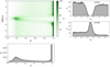Fig. 4. Study of the statistical power of $\widehat{p}(m=1|x_{\mathrm{obs}})$ to detect short-term variations with respect to the value of rSFR. Top left panel: joint distribution of $\widehat{p}(m=1|x_{\mathrm{obs}})$ and rSFR. Bottom left panel: distribution of $\widehat{p}(m=1|x_{\mathrm{obs}})$ obtained with x coming from the test catalog. Right panels: marginal distributions of rSFR for mock sources with $\widehat{p}(m=1|x_{\mathrm{obs}})>0.97$ (top right panel) and for mock sources with $\widehat{p}(m=1|x_{\mathrm{obs}})<0.4$ (bottom right panel).

The distribution (Fig. 4, bottom left panel) has two peaks, one centered around p = 0.2 and one between 0.97 and 1. This peak at 0.2, and not 0, is expected when one of the models proposed to the choice is included in the second model. In the distribution of the $\widehat{p}(m=1|x_{\mathrm{obs}})$, 20% of the sources have a value higher than 0.97 and 52% lower than 0.4. In the right panels of Fig. 4 we show the distribution of r_SFR for the galaxies x with $\widehat{p}(m=1|x_{\mathrm{obs}})>0.97$. With a perfect method, galaxies with r_SFR ≠ 1 should have $\widehat{p}(m=1|x_{\mathrm{obs}})=1$. Here we see indeed a deficit of galaxies around p = 1, but the range of affected r_SFR extends from 0.1 to 10. This shows that the method is not able to identify galaxies with an SFR variability if this variability is only 0.1–10 times the SFR before the variability began. In other words, the method is sensitive to | log r_SFR| > 1. This is confirmed by the distribution of r_SFR for galaxies with p <  0.40 (Fig. 4, bottom panel). However, there are sources with a | log r_SFR| > 1 that is associated with low values of $\widehat{p}(m=1|x_{\mathrm{obs}})$. The complete distribution of r_SFR as a function of $\widehat{p}(m=1|x_{\mathrm{obs}})$ is shown in Fig. 4.

4.2. Importance of particular flux ratios

We determined which part of the dataset x most influences the choice of SFH given by our method. The analysis of x relies entirely on the summary statistics S(x), the flux ratios. We therefore tried to understand which flux ratios are most discriminant for the model choice. We wished to verify that the method is not based on a bias of our simulations and to assess which part of the data could be removed without losing crucial information.

We used different usual metrics (e.g., Friedman et al. 2001; Chen & Guestrin 2016) to assess the importance of each flux ratio in the machine-learning estimation of $\widehat{p}(m=1|x)$. These metrics are used as indicators of the relevance of each flux ratio for the classification task. As expected, the highest flux ratios for our problem involve the bands at shortest wavelength (FUV at z <  0.68 and NUV above because FUV is no longer available), normalized by either Ks or u. This is expected because these bands are known to be sensitive to SFH (e.g., Arnouts et al. 2013). We see no particular pattern in the estimated importance of the other flux ratios. They were all used for the classification, and removing any of them decreases the classification accuracy, except for IRAC1/Ks, whose importance is consistently negligible across every considered metric.

We also tested whether the UVJ selection we used to classify galaxies according to their star formation activity (e.g., Wuyts et al. 2007; Williams et al. 2009) is able to probe the type of rapid and recent SFH variations we investigate here. We trained an XGBoost classification model using only u/V and V/J in order to evaluate the benefits of using all available flux ratios. This resulted in a severe increase in classification error, which increased from 21.0% using every flux ratios to 35.8%.

4.3. Comparison with SED fitting methods based on the BIC

In this section we compare the results obtained with the ABC method to those obtained with a standard SED modeling. The goal of this test is to understand and quantify the improvement that the ABC method brings in terms of result accuracy. We used the simulated catalog of 30 000 sources, described at the beginning of this section, for which we controlled all parameters.

The ABC method was also used on this additional catalog. This test is very similar to the training procedure described in Sect. 4.1. With this additional catalog, the ABC method has an error rate of 21.2% compared to 21.0% with the previous test sample.

CIGALE was run on the test catalog as well. The set of modules was the same as the set we used to create the mock SEDs, but the parameters we used to fit the test catalog did not include the input parameters, which were chosen randomly. This test was intentionally thought to be simple and represent an ideal case scenario. The error rate that was obtained with CIGALE therefore represents the best achievable result.

To decide whether a flexible SFH was preferable to a normal delayed-τ SFH using CIGALE, we adopted the method of Ciesla et al. (2018) described in Sect. 2.1. The quality of fit using each SFH was tested through the use of the BIC.

In detail, the method we used was the following: First, we performed a run with CIGALE using a simple delayed-τ SFH whose parameters are presented in Table 6. A second run was then performed with the flexible SFH. We compared the results and quality of the fits using one SFH or the other. The two models have different numbers of degrees of freedom. To take this into account, we computed the BIC presented in Sect. 3.2 for each SFH.

We then calculated the difference between BIC_delayed and BIC_flex (ΔBIC) and used the threshold defined by Jeffreys (Sect. 3.2), which is valid either for the BF and the BIC and was also used in Ciesla et al. (2018): a ΔBIC larger than 10 is interpreted as a strong difference between the two fits (Kass & Raftery 1995), with the flexible SFH providing a better fit of the data than the delayed-τ SFH.

We applied this method to the sample containing 15k sources modeled with a delayed-τ SFH and 15k modeled using a delayed-τ + flexibility. With these criteria, we find that the error rate of CIGALE, in terms of identifying SEDs built with a delayed-τ + flex SFH, is 32.5%. This rate depends on the ΔBIC threshold chosen and increases with the value of the threshold, as shown in Fig. 5. The best value, 28.7%, is lower than the error rate obtained from a logistic regression or an LDA (see Table 4) but is significantly higher than the error rate obtained from our procedure using XGBoost (21.0%). In this best-case scenario test for CIGALE, a difference of 7.7% is substantial and implies that the ABC method tested in this study provides better results than a more traditional one using SED fitting. When considering sources with ΔBIC > 10, that is, sources for which the method using CIGALE estimates that there is strong evidence for the flexible SFH, 95.4% are indeed SEDs simulated with the flexible SFH. Using our procedure with XGBoost and the Bayes factor corresponding threshold of 150 (Kass & Raftery 1995), we find that 99.7% of the source SFHs are correctly identified. The ABC method provides a cleaner sample than the CIGALE ΔBIC-based method.

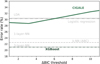Fig. 5. Error rate obtained with CIGALE as a function of the ΔBIC chosen threshold. For comparison we show the error rates obtained by the classification methods tested in Sect. 3.

5. Application on COSMOS data

We now apply our method to the sample of galaxies drawn from the COSMOS catalog, whose selection is described in Sect. 2.2. As a result, we show the $\widehat{p}(m=1|x_{\mathrm{obs}})$ distribution obtained for this sample of observed galaxies in Fig. 6. We recall that the 0 value indicates that the delayed-τ SFH is preferred, whereas $\widehat{p}=1$ indicates that the flexible SFH is more adapted to fit the SED of the galaxy. As a guide, we indicate the different grades of the Jeffreys scale and provide the number of sources in each grade in Table 7. The flexible SFH models the observations of 16.4% of our sample better than the delayed-τ SFH. However, this also means that for most of the dataset (83.6%), there is no strong evidence for a necessity to increase the complexity of the SFH; a delayed-τ is sufficient to model the SED of these sources.

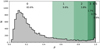Fig. 6. Distribution of the predictions $\widehat{p}(m=1|x_{\mathrm{obs}})$ produced by our algorithm on the selected COSMOS data. Sources with a $\widehat{p}(m=1|x_{\mathrm{obs}})$ close to 1 tend to prefer the delayed-τ + flex SFH, while sources with lower $\widehat{p}(m=1|x_{\mathrm{obs}})$ favor a simple delayed-τ SFH. The green regions numbered from 1 to 5 indicate the Jeffreys scale of the Bayes factor, 1: barely worth mentioning, 2: substantial, 3: strong, 4: very strong, and 5: decisive (detailed at the end of Sect. 3.2). The percentage of sources in each grade is provided in the figure and in Table 7.

To investigate the possible differences in terms of physical properties of galaxies according to their Jeffreys grade, we divided the sample of galaxies into two groups. The first group corresponds to galaxies with $\widehat{p}(m=1|x_{\mathrm{obs}})<0.5$, galaxies for which there is no evidence for the need of a recent burst or quenching in the SFH, a delayed-τ SFH is sufficient to model the SED of these sources. We selected the galaxies of the second group imposing $\widehat{p}(m=1|x_{\mathrm{obs}})>0.75$, that is, Jeffreys scale grades of 3, 4, or 5: from strong to decisive evidence against the normal delayed-τ. In Fig. 7 (top panel) we show the stellar mass distribution of the two subsamples. Although the stellar masses obtained with either the smooth delayed-τ or the flexible SFH are consistent with each other, for each galaxy we used the most suitable stellar mass: if the galaxy had $\widehat{p}(m=1|x_{\mathrm{obs}})<0.5$, the stellar mass obtained from the delayed-τ SFH was used, and if the galaxy had $\widehat{p}(m=1|x_{\mathrm{obs}})>0.75$, the stellar mass obtained with the flexible SFH was used. The stellar mass distribution of galaxies with a delayed-τ SFH is similar to the distribution of the whole sample, as shown in the middle panel of Fig. 7. However, the stellar mass distribution of galaxies needing a flexibility in their recent SFH shows a deficit of galaxies with stellar masses between 10^9.5 and 10^10.5 M_⊙ compared to the distribution of the fool sample. We note that at masses hiher than 10^10.5 M_⊙ the distribution are identical, despite a small peak at 10^11.1 M_⊙. To verify that this results is not due to our SED modeling procedure and the assumptions we adopted, we show in the middle panel of Fig. 7 the same stellar mass distributions, this time using the values published by Laigle et al. (2016). The two stellar mass distributions, with the one of galaxies with $\widehat{p}(m=1|x_{\mathrm{obs}})>0.75$ peaking at a lower mass, are recovered. This implies that these differences between the distributions are independent of the SED fitting method that is employed to determine the stellar mass of the galaxies. We note that when the algorithm has been trained, only ratios of fluxes were provided to remove the normalization factor out of the method, and the mock SEDs from which the flux ratios were computed were all normalized to 1 M_⊙. The stellar mass is at first order a normalization through, for instance, the L_K − M_* relation (e.g., Gavazzi et al. 1996). When flux ratios were used, the algorithm had no information linked to the stellar mass of the mock galaxies. Nevertheless, applied to real galaxies, the result of our procedure yields two different stellar mass distributions between galaxies identified as having smooth SFH and galaxies undergoing a more drastic episode (star formation burst or quenching).

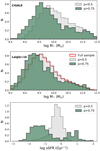Fig. 7. Top panel: comparison of the stellar mass distribution obtained with CIGALE for the sample of galaxies with $\widehat{p}(m=1|x_{\mathrm{obs}})>=0.75$ (green) and galaxies with $\widehat{p}(m=1|x_{\mathrm{obs}})<0.5$ (gray). Middle panel: comparison of the stellar mass distribution obtained by Laigle et al. (2016) for the sample of galaxies with $\widehat{p}(m=1|x_{\mathrm{obs}})>=0.75$ (green) and galaxies with $\widehat{p}(m=1|x_{\mathrm{obs}})<0.5$ (gray). Bottom panel: comparison of the sSFR distribution for the sample of galaxies with $\widehat{p}(m=1|x_{\mathrm{obs}})>=0.75$ (green) and galaxies with $\widehat{p}(m=1|x_{\mathrm{obs}})<0.5$ (gray).

In the bottom panel of Fig. 7 we show the distribution in specific star formation rate (sSFR, sSFR ≡ SFR/M_*) for the same two samples. The distribution of galaxies with $\widehat{p}(m=1|x_{\mathrm{obs}})<0.5$ is narrow (σ = 0.39) and has one peak at log sSFR = −0.32 (Gyr⁻¹), clearly showing the MS of star-forming galaxies. Galaxies with a high probability to have a recent strong variation in their SFH form a double-peaked distribution with one peak above the MS that is formed by galaxies with $\widehat{p}(m=1|x_{\mathrm{obs}})>0.75$ (log sSFR = 0.66), corresponding to galaxies having experienced a recent burst, and a second peak at lower sSFRs than the MS, corresponding to sources having undergone a recent decrease in their star formation activity (log sSFR = −1.38). In the sample of galaxies with $\widehat{p}(m=1|x_{\mathrm{obs}})>0.75$, 28% of these sources are in the peak of galaxies experiencing a burst of star formation activity and 72% seem to undergo a rapid and drastic decrease of their SFR. One possibility to explain this asymmetry could be a bias produced by the algorithm, as shown in Fig. 4, more sources with $\widehat{p}(m=1|x_{\mathrm{obs}})>0.97$ tend to be associated with low values of r_SFR than with r_SFR >  1. However, in the case of the additional catalog, this disparity is 47% and 53% for high and low r_SFR, respectively.

The distribution of the two samples in terms of sSFR indicates that to be able to reach the sSFR of galaxies that are outside the MS, a flexibility in the SFH of galaxies had to be taken into acount when the SED modeling was performed. This is needed to recover the parameter space in SFR and M_* as far as possible.

6. Conclusions

In this pilot study, we proposed to use a custom statistical method using a machine-learning algorithm, the approximate Bayesian computation, to determine the best-suited SFH to be used to measure the physical properties of a subsample of COSMOS galaxies. These galaxies were selected in mass (log M_* >  8.5) and redshift (0.5 <  z <  1). Furthermore, we imposed that the galaxies should be detected in all UV-to-NIR bands with an S/N higher than 10. We verified that these criteria do not bias the sSFR distribution of the sample.

To model these galaxies, we considered a smooth delayed-τ SFH with or without a rapid and drastic change in the recent SFH, that is, in the last few hundred million years. We built a mock galaxy SED using the SED-fitting code CIGALE. The mock SEDs were integrated into the COSMOS set of broadband filters. To avoid large dynamical ranges of fluxes, which is to be avoided when classification algorithms are used, we computed flux ratios.

Different classification algorithms were tested with XGBoost and provided the best results with a classification error of 20.98%. As output, the algorithm provides the probability that a galaxy is better modeled using a flexibility in the recent SFH. The method is sensitive to variations in SFR that are larger than 1 dex.

We compared the results from the ABC new method with SED-fitting using CIGALE. Following the method proposed by Ciesla et al. (2018), we compared the results of two SED fits, one using the delayed-τ SFH and the other adding a flexibility in the recent history of the galaxy. The BIC was computed and compared to determine which SFH provided a better fit. The BIC method provides a high error rate, 28%, compared to the 21% obtained with the ABC method. Moreover, because the BIC method requires two SED fits per analysis of a source, it is much slower than the proposed ABC method: we were not able to compare them on the test catalog of 200 000 sources, and we had to introduce a smaller simulated catalog of 30 000 sources to compute their BIC in a reasonable amount of time.

We used the result of the ABC method to determine the stellar mass and SFRs of the galaxies using the best-suited SFH for each of them. We compared two samples of galaxies: the first was galaxies with $\widehat{p}(m=1|x_{\mathrm{obs}})<0.5$, which are galaxies for which the smooth delayed-τ SFH is preferred, the second sample was galaxies with $\widehat{p}(m=1|x_{\mathrm{obs}})>0.75$, that is, galaxies for which there is strong to decisive evidence against the smooth delayed-τ SFH. The stellar mass distribution of these two samples is different. The mass distribution of galaxies for which the delayed-τ SFH is preferred is similar to the distribution of the whole sample. However, the mass distribution of galaxies that required a flexible SFH shows a deficit between 10^9.5 and 10^10.5 M_⊙. Their distribution is similar to that of the whole sample above M_* = 10^10.5 M_⊙, however. Furthermore, the results of this study also imply that a flexible SFH is required to cover the largest parameter space in terms of stellar mass and SFR, as seen from the sSFR distributions of galaxies with $\widehat{p}(m=1|x_{\mathrm{obs}})>0.75$.

Acknowledgments

The authors thank Denis Burgarella and Yannick Roehlly for fruitful discussions and the referee for his valuable comments that helped improve the paper. The research leading to these results was partially financed via the PEPS Astro-Info program of the CNRS. P. Pudlo warmly thanks the Centre International de Rencontres Mathématiques (CIRM) of Aix-Marseille University for its support and the stimulating atmosphere during the Jean Morlet semester “Bayesian modeling and Analysis of Big Data” chaired by Kerrie Mengersen.

References

Appendix A: Effect of flux S/N on the distribution of p(x_obs|m = 1)

In Fig. A.1 we show the distribution of the estimated probability $\widehat{p}(m=1|x_{\mathrm{obs}})$ for the subsample of COSMOS sources described in Sect. 2.2 before any S/N cuts are applied. In this figure, all COSMOS sources with M_* >  10^8.5 M_⊙ and redshift between 0.5 and 1 are used. The 0 value indicates that the delayed-τ SFH is preferred, whereas $\widehat{p}=1$ indicates that the delayed-τ + flex SFH is more adapted to fit the SED of the galaxy. To understand what drives the shape of the $\widehat{p}(m=1|x_{\mathrm{obs}})$ distribution, we show in the same figure the distributions obtained for different Ks S/N bins (top panel) and NUV S/N bins (bottom panel). Galaxies with low S/N in either NUV and Ks photometric band show flatter $\widehat{p}(m=1|x_{\mathrm{obs}})$ distributions. This means that these low S/N sources yield intermediate values of $\widehat{p}(m=1|x_{\mathrm{obs}})$, translating into a difficulty of choosing between the delayed-τ and the delayed-τ + flex SFHs.

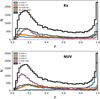Fig. A.1. Distribution of the predictions $\widehat{p}(m=1|x_{\mathrm{obs}})$ as a function of Ks band S/N (top panel) and NUV S/N (bottom panel). The different colors are for different selections in S/N in each panel.

Appendix B: Bayesian evidence

The evidence p(x_obs|m) is a normalized probability density that represents the distribution of datasets drawn from the mth model, regardless of the value of the parameter θ_m from its prior distribution. If models m = 0 and m = 1 are nested, the region of the data space of non-negligible probability under model m = 0 has also a non-negligible probability under model m = 1. Moreover, because model m = 1 can fit to many more datasets, the probability density p(x_obs|m = 1) is much more diffuse than the density p(x_obs|m = 0). We therefore expect for datasets x that can be explained by both models m = 0, 1 that p(x|m = 1) ≤ p(x|m = 0). If the prior probabilities p(m = 0) and p(m = 1) of both models are equal, it implies that for datasets x_obs that can be explained by both models, p(m = 1|x) ≤ p(m = 0|x).

Appendix C: Parameter tuning for classification methods

The training catalog was used to optimize the value of ϕ with a specific algorithm given ψ, and the validation catalog was used to fit the tuning parameters ψ. To fit ϕ to a catalog of simulated datasets (mⁱ, xⁱ), i ∈ I, the optimization algorithm specified with the machine-learning model maximizes

$$\begin{array}{c}\hfill {\displaystyle \prod _{i\in I}L(\widehat{p}(m=1|x^i);m^i),\mathrm{where}L(p;m)=\{\begin{array}{cc}p\hfill & \mathrm{if}m=1,\hfill \\ (1-p)\hfill & \mathrm{if}m=0,\hfill \end{array}}\end{array}$$

given the value of ψ. Generally, this optimization algorithm was run for several values of ψ. Then, the validation catalog was used to calibrate the tuning parameters ψ based on data: the accuracy of ${\widehat{p}}_{\psi }(m=1|x)$ for many possible values of ψ was computed on the validation catalog, and we selected the value $\widehat{\psi }$ that led to the best results on this catalog. The resulting output of this two-step procedure is the approximation ${\widehat{p}}_{\widehat{\psi }}(m|x)$, which can easily be evaluated for the new dataset x′. The accuracy of $\widehat{p}(m=1|x)$ can be measured with various metrics. The most common metric is the classification error rate on a catalog of (m^j, S(x^j)), j ∈ J, of |J| simulations. We relied on this metric. It is is defined by the frequency at which the datasets x^j are not well classified, that is,

$$\begin{array}{c}\hfill \frac{1}{|J|}{\displaystyle \sum _{j\in J}}\mathbf{1}\{{\widehat{m}}^j\ne m^j\},\mathrm{where}{\widehat{m}}^j=\{\begin{array}{cc}1\hfill & \mathrm{if}\widehat{p}(m=1|x^j)>1/2.\hfill \\ 0\hfill & \mathrm{if}\widehat{p}(m=1|x^j)\le 1/2.\hfill \end{array}\end{array}$$

All Tables

All Figures

Fig. 1. Examples of delayed-τ SFHs considered in this work (star formation rate as a function of cosmic time). Different SFHs using τmain = 0.5, 1, 5, and 10 Gyr are shown to illustrate the effect of this parameter (light green and dark green solid lines). An example of a delayed-τ SFH with flexibility is shown in solid dark green, with the flexibility as green dashed lines for (ageflex = 1 Gyr and rSFR = 0.3) and (ageflex = 0.5 Gyr and rSFR = 7).

In the text

	Fig. 2. Stellar mass from Laigle et al. (2016) as a function of redshift for the final sample (top panel) and for the rejected galaxies following our criteria (bottom panel).
In the text

	Fig. 3. Distribution of stellar mass for the sample before the S/N cut (gray) and the final sample (green). The red dotted line indicates the limit above which our final sample is considered complete. The stellar masses indicated here are from Laigle et al. (2016).
In the text

Fig. 4. Study of the statistical power of $\widehat{p}(m=1|x_{\mathrm{obs}})$ to detect short-term variations with respect to the value of rSFR. Top left panel: joint distribution of $\widehat{p}(m=1|x_{\mathrm{obs}})$ and rSFR. Bottom left panel: distribution of $\widehat{p}(m=1|x_{\mathrm{obs}})$ obtained with x coming from the test catalog. Right panels: marginal distributions of rSFR for mock sources with $\widehat{p}(m=1|x_{\mathrm{obs}})>0.97$ (top right panel) and for mock sources with $\widehat{p}(m=1|x_{\mathrm{obs}})<0.4$ (bottom right panel).

In the text

	Fig. 5. Error rate obtained with CIGALE as a function of the ΔBIC chosen threshold. For comparison we show the error rates obtained by the classification methods tested in Sect. 3.
In the text

Fig. 6. Distribution of the predictions $\widehat{p}(m=1|x_{\mathrm{obs}})$ produced by our algorithm on the selected COSMOS data. Sources with a $\widehat{p}(m=1|x_{\mathrm{obs}})$ close to 1 tend to prefer the delayed-τ + flex SFH, while sources with lower $\widehat{p}(m=1|x_{\mathrm{obs}})$ favor a simple delayed-τ SFH. The green regions numbered from 1 to 5 indicate the Jeffreys scale of the Bayes factor, 1: barely worth mentioning, 2: substantial, 3: strong, 4: very strong, and 5: decisive (detailed at the end of Sect. 3.2). The percentage of sources in each grade is provided in the figure and in Table 7.

In the text

Fig. 7. Top panel: comparison of the stellar mass distribution obtained with CIGALE for the sample of galaxies with $\widehat{p}(m=1|x_{\mathrm{obs}})>=0.75$ (green) and galaxies with $\widehat{p}(m=1|x_{\mathrm{obs}})<0.5$ (gray). Middle panel: comparison of the stellar mass distribution obtained by Laigle et al. (2016) for the sample of galaxies with $\widehat{p}(m=1|x_{\mathrm{obs}})>=0.75$ (green) and galaxies with $\widehat{p}(m=1|x_{\mathrm{obs}})<0.5$ (gray). Bottom panel: comparison of the sSFR distribution for the sample of galaxies with $\widehat{p}(m=1|x_{\mathrm{obs}})>=0.75$ (green) and galaxies with $\widehat{p}(m=1|x_{\mathrm{obs}})<0.5$ (gray).

In the text

	Fig. A.1. Distribution of the predictions $\widehat{p}(m=1|x_{\mathrm{obs}})$ as a function of Ks band S/N (top panel) and NUV S/N (bottom panel). The different colors are for different selections in S/N in each panel.
In the text

References

- Abramson, L. E., Gladders, M. D., Dressler, A., et al. 2016, ApJ, 832, 7 [NASA ADS] [CrossRef] [Google Scholar]
- Arnouts, S., Le Floc’h, E., Chevallard, J., et al. 2013, A&A, 558, A67 [NASA ADS] [CrossRef] [EDP Sciences] [Google Scholar]
- Behroozi, P. S., Wechsler, R. H., & Conroy, C. 2013, ApJ, 770, 57 [NASA ADS] [CrossRef] [Google Scholar]
- Boquien, M., Buat, V., & Perret, V. 2014, A&A, 571, A72 [NASA ADS] [CrossRef] [EDP Sciences] [Google Scholar]
- Boquien, M., Burgarella, D., Roehlly, Y., et al. 2019, A&A, 622, A103 [NASA ADS] [CrossRef] [EDP Sciences] [Google Scholar]
- Boselli, A., Roehlly, Y., Fossati, M., et al. 2016, A&A, 596, A11 [NASA ADS] [CrossRef] [EDP Sciences] [Google Scholar]
- Breiman, L. 2001, Mach. Learn., 45, 5 [CrossRef] [Google Scholar]
- Bruzual, G., & Charlot, S. 2003, MNRAS, 344, 1000 [NASA ADS] [CrossRef] [Google Scholar]
- Buat, V., Heinis, S., Boquien, M., et al. 2014, A&A, 561, A39 [NASA ADS] [CrossRef] [EDP Sciences] [Google Scholar]
- Calzetti, D., Armus, L., Bohlin, R. C., et al. 2000, ApJ, 533, 682 [NASA ADS] [CrossRef] [Google Scholar]
- Carnall, A. C., Leja, J., Johnson, B. D., et al. 2019, ApJ, 873, 44 [NASA ADS] [CrossRef] [Google Scholar]
- Charlot, S., & Fall, S. M. 2000, ApJ, 539, 718 [NASA ADS] [CrossRef] [Google Scholar]
- Chen, T., & Guestrin, C. 2016, Proceedings of the 22nd ACM SIGKDD International Conference on Knowledge Discovery and Data Mining (ACM), 785 [Google Scholar]
- Ciesla, L., Charmandaris, V., Georgakakis, A., et al. 2015, A&A, 576, A10 [NASA ADS] [CrossRef] [EDP Sciences] [Google Scholar]
- Ciesla, L., Boselli, A., Elbaz, D., et al. 2016, A&A, 585, A43 [NASA ADS] [CrossRef] [EDP Sciences] [Google Scholar]
- Ciesla, L., Elbaz, D., & Fensch, J. 2017, A&A, 608, A41 [NASA ADS] [CrossRef] [EDP Sciences] [Google Scholar]
- Ciesla, L., Elbaz, D., Schreiber, C., Daddi, E., & Wang, T. 2018, A&A, 615, A61 [NASA ADS] [CrossRef] [EDP Sciences] [Google Scholar]
- Dekel, A., & Burkert, A. 2014, MNRAS, 438, 1870 [NASA ADS] [CrossRef] [Google Scholar]
- Elbaz, D., Daddi, E., Le Borgne, D., et al. 2007, A&A, 468, 33 [NASA ADS] [CrossRef] [EDP Sciences] [Google Scholar]
- Friedman, J., Hastie, T., & Tibshirani, R. 2001, The Elements of Statistical Learning (New York: Springer-Verlag) [Google Scholar]
- Gavazzi, G., Pierini, D., & Boselli, A. 1996, A&A, 312, 397 [NASA ADS] [Google Scholar]
- Gladders, M. D., Oemler, A., Dressler, A., et al. 2013, ApJ, 770, 64 [NASA ADS] [CrossRef] [Google Scholar]
- Guo, K., Zheng, X. Z., & Fu, H. 2013, ApJ, 778, 23 [NASA ADS] [CrossRef] [Google Scholar]
- Ilbert, O., Arnouts, S., Le Floc’h, E., et al. 2015, A&A, 579, A2 [NASA ADS] [CrossRef] [EDP Sciences] [Google Scholar]
- Kass, R. E., & Raftery, A. E. 1995, J. Am. Stat. Assoc., 90, 773 [CrossRef] [Google Scholar]
- Laigle, C., McCracken, H. J., Ilbert, O., et al. 2016, ApJS, 224, 24 [NASA ADS] [CrossRef] [Google Scholar]
- Lee, S.-K., Ferguson, H. C., Somerville, R. S., Wiklind, T., & Giavalisco, M. 2010, ApJ, 725, 1644 [NASA ADS] [CrossRef] [EDP Sciences] [Google Scholar]
- Leja, J., Carnall, A. C., Johnson, B. D., Conroy, C., & Speagle, J. S. 2019, ApJ, 876, 3 [Google Scholar]
- Magdis, G. E., Daddi, E., Béthermin, M., et al. 2012, ApJ, 760, 6 [NASA ADS] [CrossRef] [Google Scholar]
- Maraston, C. 2005, MNRAS, 362, 799 [NASA ADS] [CrossRef] [Google Scholar]
- Maraston, C., Pforr, J., Renzini, A., et al. 2010, MNRAS, 407, 830 [NASA ADS] [CrossRef] [Google Scholar]
- Marin, J.-M., Pudlo, P., Robert, C. P., & Ryder, R. J. 2012, Stat. Comput., 22, 1167 [Google Scholar]
- Marin, J. M., Pudlo, P., Estoup, A., & Robert, C. 2018, in Handbook of Approximate Bayesian Computation, eds. S. A. Sisson, Y. Fan, & M. Beaumont (Chapman and Hall/CRC) [Google Scholar]
- Niculescu-Mizil, A., & Caruana, R. 2012, ArXiv e-prints [arXiv:1207.1403] [Google Scholar]
- Noeske, K. G., Weiner, B. J., Faber, S. M., et al. 2007, ApJ, 660, L43 [Google Scholar]
- Pacifici, C., Kassin, S. A., Weiner, B., Charlot, S., & Gardner, J. P. 2013, ApJ, 762, L15 [NASA ADS] [CrossRef] [Google Scholar]
- Pacifici, C., Oh, S., Oh, K., Lee, J., & Yi, S. K. 2016, ApJ, 824, 45 [NASA ADS] [CrossRef] [EDP Sciences] [Google Scholar]
- Papovich, C., Dickinson, M., & Ferguson, H. C. 2001, ApJ, 559, 620 [NASA ADS] [CrossRef] [Google Scholar]
- Pforr, J., Maraston, C., & Tonini, C. 2012, MNRAS, 422, 3285 [NASA ADS] [CrossRef] [Google Scholar]
- Pudlo, P., Marin, J.-M., Estoup, A., et al. 2016, Bioinformatics, 32, 859 [CrossRef] [Google Scholar]
- Robert, C. 2007, The Bayesian Choice: From Decision Theoretic Foundations to Computational Implementation (Springer Science & Business Media) [Google Scholar]
- Salmi, F., Daddi, E., Elbaz, D., et al. 2012, ApJ, 754, L14 [NASA ADS] [CrossRef] [Google Scholar]
- Sargent, M. T., Daddi, E., Béthermin, M., et al. 2014, ApJ, 793, 19 [NASA ADS] [CrossRef] [Google Scholar]
- Schreiber, C., Pannella, M., Elbaz, D., et al. 2015, A&A, 575, A74 [NASA ADS] [CrossRef] [EDP Sciences] [Google Scholar]
- Scoville, N., Sheth, K., Aussel, H., et al. 2016, ApJ, 820, 83 [NASA ADS] [CrossRef] [Google Scholar]
- Simha, V., Weinberg, D. H., Conroy, C., et al. 2014, ArXiv e-prints [arXiv:1404.0402] [Google Scholar]
- Sisson, S. A., Fan, Y., & Beaumont, M. 2018, Handbook of Approximate Bayesian Computation (Chapman and Hall/CRC) [CrossRef] [Google Scholar]
- Tacchella, S., Dekel, A., Carollo, C. M., et al. 2016, MNRAS, 458, 242 [NASA ADS] [CrossRef] [Google Scholar]
- Vehtari, A., & Ojanen, J. 2012, Stat. Surv., 6, 142 [CrossRef] [Google Scholar]
- Williams, R. J., Quadri, R. F., Franx, M., van Dokkum, P., & Labbé, I. 2009, ApJ, 691, 1879 [NASA ADS] [CrossRef] [Google Scholar]
- Wuyts, S., Labbé, I., Franx, M., et al. 2007, ApJ, 655, 51 [NASA ADS] [CrossRef] [Google Scholar]
- Wuyts, S., Förster Schreiber, N. M., van der Wel, A., et al. 2011, ApJ, 742, 96 [NASA ADS] [CrossRef] [Google Scholar]