© ESO, 2015

1. Introduction

Weak lensing (WL) is a gravitational deflection effect of light by matter inhomogeneities in the Universe that causes distortion of source galaxy images. This distortion corresponds to the integrated deflection along the line of sight, and its measurement probes the high-mass regions of the Universe. These regions contain structures that formed during the late-time evolution of the Universe, which depends on cosmological parameters, such as the matter density parameter Ω_m, the matter density fluctuation σ₈, and the equation of state of dark energy w. Ongoing and future surveys such as KiDS¹, DES², HSC³, WFIRST⁴, Euclid⁵, and LSST⁶ are expected to provide tight constraints on those and other cosmological parameters and to distinguish between different cosmological models, using weak lensing as a major probe.

Lensing signals can be extracted in several ways. A common observable is the cosmic shear two-point-correlation function (2PCF), which has been used to constrain cosmological parameters in many studies, including recent ones (Kilbinger et al. 2013; Jee et al. 2013). However, the 2PCF only retains Gaussianity, and it misses the rich nonlinear information of the structure evolution encoded on small scales. To compensate for this drawback, several non-Gaussian statistics have been proposed, for example higher order moments (Kilbinger & Schneider 2005; Semboloni et al. 2011; Fu et al. 2014; Simon et al. 2015), the three-point correlation function (Schneider & Lombardi 2003; Takada & Jain 2003; Scoccimarro et al. 2004), Minkowski functionals (Petri et al. 2015), or peak statistics, which is the aim of this series of papers. Some more general work comparing different strategies to extract non-Gaussian information can be found in the literature (Pires et al. 2009, 2012; Bergé et al. 2010).

Peaks, defined as local maxima of the lensing signal, are direct tracers of high-mass regions in the large-scale structure of the Universe. In the medium and high signal-to-noise (S/N) regime, the peak function (the number of peaks as function of S/N) is not dominated by shape noise, and this permits one to study the cosmological dependency of the peak number counts (Jain & Van Waerbeke 2000). Various aspects of peak statistic have been investiagated in the past: the physical origin of peaks (Hamana et al. 2004; Yang et al. 2011), projection effects (Marian et al. 2010), the optimal combination of angular scales (Kratochvil et al. 2010; Marian et al. 2012), redshift tomography (Hennawi & Spergel 2005), cosmological parameter constraints (Dietrich & Hartlap 2010; Liu, X. et al. 2014), detecting primordial non-Gaussianity (Maturi et al. 2011; Marian et al. 2011), peak statistics beyond the abundance (Marian et al. 2013), the impact from baryons (Yang et al. 2013; Osato et al. 2015), magnification bias (Liu, J. et al. 2014), and shape measurement errors (Bard et al. 2013). Recent studies byLiu et al. (2015, hereafterLPH15),Liu et al. (2015, hereafter LPL15), and Hamana et al. (2015) have applied likelihood estimation for WL peaks on real data and have shown that the results agree with the current ΛCDM scenario.

Modeling number counts is a challenge for peak studies. To date, there have been three main approaches. The first one is to count peaks from a large number of N-body simulations (Dietrich & Hartlap 2010; LPH15), which directly emulate structure formation by numerical implementation of the corresponding physical laws. The second family consists of analytic predictions (Maturi et al. 2010; Fan et al. 2010) based on Gaussian random field theory. A third approach has been introduced by Lin & Kilbinger (2015, hereafter Paper I: similar to Kruse & Schneider (1999) and Kainulainen & Marra (2009, 2011a,b), we propose a stochastic process to predict peak counts by simulating lensing maps from a halo distribution drawn from the mass function.

Our model possesses several advantages. The first one is flexibility. Observational conditions can easily be modeled and taken into account. The same is true for additional features, such as intrinsic alignment of galaxies and other observational and astrophysical systematics. Second, since our method does not need N-body simulations, the computation time required to calculate the model are orders of magnitudes faster, and we can explore a large parameter space. Third, our model explores the underlying probability density function (PDF) of the observables. All statistical properties of the peak function can be derived directly from the model, making various parameter estimation methods possible.

In this paper, we apply several parameter constraint and likelihood methods for our peak-count-prediction model from Paper I. Our goal is to study and compare different strategies and to make use of the full potential of the fast stochastic forward modeling approach. We start with a likelihood function that is assumed to be Gaussian in the observables with constant covariance and then compare this to methods that make fewer and fewer assumptions, as follows.

The first extension of the Gaussian likelihood is to take the cosmology-dependent covariances (CDC, see Eifler et al. 2009) into account. Thanks to the fast performance of our model, it is feasible to estimate the covariance matrix for each parameter set.

The second improvement we adopt is the copula analysis (Benabed et al. 2009; Jiang et al. 2009; Takeuchi 2010; Scherrer et al. 2010; Sato et al. 2011) for the Gaussian approximation. Widely used in finance, the copula transform uses the fact that any multivariate distribution can be transformed into a new one where the marginal PDF is uniform. Combining successive transforms can then give rise to a new distribution where all marginals are Gaussian. This makes weaker assumptions about the underlying likelihood than the Gaussian hypothesis.

Third, we directly estimate the full underlying distribution information in a non-analytical way. This allows us to strictly follow the original definition of the likelihood estimator: the conditional probability of observables for a given parameter set. In addition, we compute the p-value from the full PDF. These p-values derived for all parameter sets allow for significance tests and provide a direct way to construct confidence contours.

Furthermore, our model makes it possible to dispose of a likelihood function altogether, using approximate Bayesian computation (ABC, see e.g. Marin et al. 2011) for exploring the parameter space. ABC is a powerful constraining technique based on accept-reject sampling. Proposed first by Rubin (1984), ABC produces the posterior distribution by bypassing the likelihood evaluation, which may be complex and practically unfeasible in some contexts. The posterior is constructed by comparing the sampled result with the observation to decide whether a proposed parameter is accepted. This technique can be improved by combining ABC with population Monte Carlo (PMC⁷, Beaumont et al. 2009; Cameron & Pettitt 2012; Weyant et al. 2013). Until now, ABC seems to already have various applications in biology-related domains (e.g., Beaumont et al. 2009; Berger et al. 2010; Csilléry et al. 2010; Drovandi & Pettitt 2011), while applications for astronomical purposes are few: morphological transformation of galaxies (Cameron & Pettitt 2012), cosmological parameter inference using type Ia supernovae (Weyant et al. 2013), constraints of the disk formation of the Milky Way (Robin et al. 2014), and strong lensing properties of galaxy clusters (Killedar et al. 2015). Very recently, two papers (Ishida et al. 2015; Akeret et al. 2015) dedicated to ABC in a general cosmological context have been submitted.

The paper is organized as follows. In Sect. 2, we briefly review our model introduced in Paper I, the setting for the parameter analysis, and the criteria for defining parameter constraints. In Sect. 3, we study the impact of the CDC effect. The results from the copula likelihood can be found in Sects. 4, and 5 we estimate the true underlying PDF in a non-analytic way and show parameters constraints without the Gaussian hypothesis. Section 6 focuses on the likelihood-free ABC technique, and the last section is dedicated to a discussion where we summarize this work.

2. Methodology

2.1. Our model

Our peak-count model uses a probabilistic approach that generates peak catalogs from a given mass function model. This is done by generating fast simulations of halos, computing the projected mass, and simulating lensing maps from which one can extract WL peaks. A step-by-step summary is given as follows:

• 1.

  sample halo masses and assign density profiles and positions (fast simulations);

• 2.

  compute the projected mass and subtract the mean over the field (ray-tracing simulations);

• 3.

  add noise and smooth the map with a kernel; and

• 4.

  select local S/N maxima.

Here, two assumptions have been made: (1) only bound matter contributes to number counts; and (2) the spatial correlation of halos has a small impact on WL peaks. Paper I showed that combining both hypotheses gives a good estimation of the peak abundance.

We adopt the same settings as Paper I: the mass function model from Jenkins et al. (2001), the truncated Navarro-Frenk-White halo profiles (Navarro et al. 1996, 1997), Gaussian shape noise, the Gaussian smoothing kernel, and sources at fixed redshift which are distributed on a regular grid. The field of view is chosen such that the effective area after cutting off the border is 25 deg². An exhausted list of parameter values used in this paper can be found in Table 1. Readers are encouraged to read Paper I for their definitions and for detailed explanations for our model.

All computations with our model in this study are performed by our Camelus algorithm⁸. A realization (from a mass function to a peak catalog) of a 25 deg² field costs few seconds to generate on a single-CPU computer. The real time cost depends of course on input cosmological parameters, but this still gives an idea about the speed of our algorithm.

2.2. Analysis design

Throughout this paper, π denotes a parameter set. To simplify the study, the dimension of the parameter space is reduced to two: π ≡ (Ω_m,σ₈). The other cosmological parameters are fixed, including Ω_b = 0.047, h = 0.78, n_s = 0.95, and w = −1. The dark energy density Ω_de is set to 1 − Ω_m to match a flat universe. On the Ω_m-σ₈ plane, we explore a region where the posterior density, or probability, is high, see Fig. 1. We compute the values of three different log likelihoods on the grid points of these zones. The grid size of the center zone is ΔΩ_m = Δσ₈ = 0.005, whereas it is 0.01 for the rest. This results in a total of 7821 points in the parameter space to evaluate.

For each π, we carry out N = 1000 realizations of a 25 deg² field and determine the associated data vector ${{x}}^{\mathrm{\left(}\mathit{k}\mathrm{\right)}}\mathrm{=}\mathrm{\left(}{\mathit{x}}_{\mathrm{1}}^{\mathrm{\left(}\mathit{k}\mathrm{\right)}}\mathit{,}\mathit{...}\mathit{,}{\mathit{x}}_{\mathit{d}}^{\mathrm{\left(}\mathit{k}\mathrm{\right)}}\mathrm{\right)}$ for all k from 1 to N. These are independent samples drawn from their underlying PDF of observables for a given parameter π. We estimate the model prediction (which is the mean), the covariance matrix, and the inverse matrix (Hartlap et al. 2007), respectively, by following $\begin{array}{ccc}{\mathit{x}}_{\mathit{i}}^{\mathrm{mod}}& \mathrm{=}& \frac{\mathrm{1}}{\mathit{N}}\sum _{\mathit{k}\hspace{0.17em}\mathrm{=}\hspace{0.17em}\mathrm{1}}^{\mathit{N}}{\mathit{x}}_{\mathit{i}}^{\mathrm{\left(}\mathit{k}\mathrm{\right)}}\mathit{,}\\ \mathit{Ĉ}\mathit{ij}& \mathrm{=}& \frac{\mathrm{1}}{\mathit{N}\mathrm{-}\mathrm{1}}\sum _{\mathit{k}\hspace{0.17em}\mathrm{=}\hspace{0.17em}\mathrm{1}}^{\mathit{N}}\mathrm{(}{\mathit{x}}_{\mathit{i}}^{\mathrm{\left(}\mathit{k}\mathrm{\right)}}\mathrm{-}{{\mathit{x}}_{\mathit{i}}^{\mathrm{mod}}}^{\mathrm{)}}\left({\mathit{x}}_{\mathit{j}}^{\mathrm{\left(}\mathit{k}\mathrm{\right)}}\mathrm{-}{\mathit{x}}_{\mathit{j}}^{\mathrm{mod}}\right)\mathit{,}\mathrm{and}\\ \begin{array}{c}\mathrm{􏽤}\\ {{C}}^{-1}\end{array}& \mathrm{=}& \frac{\mathit{N}\mathrm{-}\mathit{d}\mathrm{-}\mathrm{2}}{\mathit{N}\mathrm{-}\mathrm{1}}{\begin{array}{c}\mathrm{􏽢}\\ {C}\end{array}}^{-1}\mathit{,}\end{array}$where d denotes the dimension of data vector. This results in a total area of 25 000 deg² for the mean estimation.

In this paper, the observation data x^obs are identified with a realization of our model, which means that x^obs is derived by a particular realization of x(πⁱⁿ). The input parameters chosen are ${{\pi }}^{\mathrm{in}}\mathrm{=}\mathrm{\left(}{\mathrm{\Omega }}_{\mathrm{m}}^{\mathrm{in}}\mathit{,}{\mathit{\sigma }}_{\mathrm{8}}^{\mathrm{in}}\mathrm{\right)}\mathrm{=}\mathrm{\left(}\mathrm{0.28}\mathit{,}\mathrm{0.82}\mathrm{\right)}$. The authors would like to highlight that the accuracy of the model is not the aim of this research work, but precision. Therefore, the input choice and the uncertainty of random process should have little impact.

Peak-count information can be combined into a data vector using different ways. Inspired by Dietrich & Hartlap (2010) and LPL15, we studied three types of observables. The first is the abundance of peaks found in each S/N bin (labeled abd), in other words, the binned peak function. The second is the S/N values at some given percentiles of the peak cumulative distribution function (CDF, labeled pct). The third is similar to the second type, but without taking peaks below a threshold S/N value (labeled cut) into account. Mathematically, the two last types of observables can be denoted as x_i, thereby satisfying $\begin{array}{ccc}{\mathit{p}}_{\mathit{i}}\mathrm{=}{\mathrm{\int }}_{{\mathit{\nu }}_{\min }}^{{\mathit{x}}_{\mathit{i}}}{\mathit{n}}_{\mathrm{peak}}\mathrm{\left(}\mathit{\nu }\mathrm{\right)}\mathrm{d}\mathit{\nu ,}& & \end{array}$(4)where n_peak(ν) is the peak PDF function, ν_min a cutoff, and p_i a given percentile. The observable x^abd is used by LPL15, while readers find x^cut from Dietrich & Hartlap (2010). We would like to clarify that using x^pct for analysis could by risky, since this includes peaks with negative S/N. From Paper I, we observe that although high-peak counts from our model agree well with N-body simulations, predictions for local maxima found in underdensity regions (peaks with S/N< 0) are inaccurate. Thus, we include x^pct in this paper only to give an idea about how much information we can extract from observables defined by percentiles.

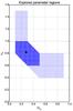Fig. 1 Location of 7821 points on which we evaluate the likelihoods. In the condensed area, the interval between two grid points is 0.005, while in both wing zones it is 0.01. The black star shows $\mathrm{\left(}{\mathrm{\Omega }}_{\mathrm{m}}^{\mathrm{in}}\mathit{,}{\mathit{\sigma }}_{\mathrm{8}}^{\mathrm{in}}\mathrm{\right)}\mathrm{=}\mathrm{\left(}\mathrm{0.28}\mathit{,}\mathrm{0.82}\mathrm{\right)}$.

Observable vectors are constructed by the description above with the settings of Table 2. This choice of bins and p_i is made such that the same component from different types of observables represents about the same information, since the bin center of x^abd5 roughly correspond to x^cut5 for the input cosmology πⁱⁿ. Following LPL15, who discovered in their study that the binwidth choice has a minor impact on parameter constraints if the estimated number count in each bin is ≳10, we chose not to explore different choices of binwidths for x^abd5. We also note that p_i for ${\mathit{x}}_{\mathit{i}}^{\mathrm{cut}\mathrm{5}}$ are logarithmically spaced.

By construction, the correlation between terms of percentile-like vectors is much higher than for the case of peak abundance. This tendency is shown in Table 3 for the πⁱⁿ cosmology. We discovered that x^pct5 and x^cut5 are highly correlated, while for x^abd5, the highest absolute value of off-diagonal terms does not exceed 17%. A similar result was observed when we binned data differently. This suggests that the covariance should be included in likelihood analyses.

2.3. Constraint qualification

In this paper, both Bayesian inferences and likelihood-ratio tests (see, e.g., Theorem 10.3.3 from Casella & Berger 2002) have been performed. To distinguish between these two cases, we call credible region the posterior PDF obtained from the Bayesian approach, which differs from the confidence region, whose interpretation can be found in Sect. 5.2.

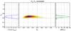Fig. 2 Middle panel: likelihood value using xabd5 on the Ωm-Σ8 plane. The green star represents the input cosmology πin. Since log σ8 and log Ωm form an approximately linear degenerency, the quantity Σ8 ≡ σ8(Ωm/ 0.27)α allows us to characterize the banana-shape contour thickness. Right panel: the marginalized PDF of Σ8. The dashed lines give the 1σ interval (68.3%), while the borders of the shaded areas represent 2σ limits (95.4%). Left panel: log-value of the marginalized likelihood ratio. Dashed lines in the left panel give the corresponding value for 1 and 2σ significance levels, respectively.

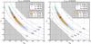Fig. 3 Confidence regions derived from Lcg, Lsvg, and Lvg with xabd5. The solid and dashed lines represent Lcg in the left panel and Lvg in the right panel, while the colored areas are from Lsvg. The black star stands for πin and gray areas represent the non-explored parameter space. The dotted lines are different isolines, the variance Ĉ55 of the bin with highest S/N in the left panel and ln(detĈ) for the right panel. The contour area is reduced by 22% when taking the CDC effect into account. The parameter-dependent determinant term does not contribute significantly.

To quantify parameter-constraint contours, we introduce two criteria. Inspired by Jain & Seljak (1997) and Maoli et al. (2001), the first criterion is to determine the error on $\begin{array}{ccc}{\mathrm{\Sigma }}_{\mathrm{8}}\mathrm{\equiv }{\mathit{\sigma }}_{\mathrm{8}}\mathrm{(}{\mathrm{\Omega }}_{\mathrm{m}}\mathit{/}\mathrm{0.27}{\mathrm{)}}^{\mathit{\alpha }}\mathit{.}& & \end{array}$(5)Since the banana-shaped contour becomes more or less an elongated ellipse in log space, ΔΣ₈ represents the “thickness” of the banana, tilted by the slope α. Therefore, we first fit α with the linear relation log Σ₈ = log σ₈ + αlog (Ω_m/ 0.27), and then calculate the 1σ interval of Σ₈ on the Ω_m-Σ₈ plane. For a Bayesian approach, this interval is given by the 68% most probable interval from the marginalized likelihood, while for a frequentist approach, significance levels are given by likelihood-ratio tests on the marginalized likelihood. Examples of both approaches are shown by Fig. 2. Since no real data are used in this study, we are not interested in the best fit value, but the 1σ interval width ΔΣ₈.

The second indicator is the figure of merit (FoM) for Ω_m and σ₈, proposed by Dietrich & Hartlap (2010). They define a FoM similar to the one from Albrecht et al. (2006) as the inverse of the area of the 2σ region.

3. Influence of the cosmology-dependent covariance

3.1. Formalism

In this section, we examine the cosmology-dependent-covariance (CDC) effect. From our statistic, we estimate the inverse covariance from Eq. (3) for each π from 1000 realizations. By setting the Bayesian evidence to unity, P(x = x^obs) = 1, we write the relation among prior probability , the likelihood ℒ(π) ≡ P(x^obs | π), and posterior probability as $\begin{array}{ccc}\mathrm{𝒫}\mathrm{\left(}{\pi }\mathrm{\right|}{{x}}^{\mathrm{obs}}\mathrm{)}\mathrm{=}\mathrm{ℒ}\mathrm{(}{\pi }\mathrm{\left)}\mathrm{𝒫}\mathrm{\right(}{\pi }\mathrm{)}\mathit{.}& & \end{array}$(6)Given a model, we write Δx(π) ≡ x^mod(π) − x^obs as the difference between the model prediction x^mod and the observation x^obs. Then the Gaussian log-likelihood is given by $\begin{array}{ccc}\mathrm{-}\mathrm{2}\ln \mathrm{ℒ}\mathrm{\left(}{\pi }\mathrm{\right)}\mathrm{=}\ln \mathrm{[}\mathrm{\left(}\mathrm{2}\mathit{\pi }{\mathrm{)}}^{\mathit{d}}\begin{array}{c}\det \end{array}\mathrm{\right(}{C}{\mathrm{)}}^{\mathrm{]}}\mathrm{+}\mathrm{\Delta }{{x}}^{\mathit{T}}{{C}}^{-1}\mathrm{\Delta }{x}& & \end{array}$(7)where d denotes the dimension of the observable space, and C is the covariance matrix for x^mod.

Estimating C as an ensemble average is difficult since cosmologists only have one Universe. One can derive C from observations with statistical techniques, such as bootstrap or jackknife (LPL15), or from a sufficient number of independent fields of view from N-body simulations (LPH15) or using analytic calculations. However, the first method only provides the estimation for a specific parameter set C(π = π^obs); the second method is limited to a small amount of parameters owing to the very high computational time cost; and the third method involves higher order statistics of the observables, which might not be well known. Thus, most studies suppose that the covariance matrix is invariant so ignore the CDC effect. In this case, the determinant term becomes a constant, and likelihood analysis can be summed up as the minimization of χ² ≡ Δx^TC^-1Δx.

Alternatively, the stochastic characteristic of our model provides a quick and simple way to estimate the covariance matrix C(π) of each single parameter set π. To examine the impact of the CDC effect in the peak-count framework, we write down the constant-covariance Gaussian (labeled cg), the semi-varying-covariance Gaussian (labeled svg), and the varying-covariance Gaussian (labeled vg) log-likelihoods as $\begin{array}{ccc}{\mathit{L}}_{\mathrm{cg}}& & \\ {\mathit{L}}_{\mathrm{svg}}& & \mathrm{\equiv }\mathrm{\Delta }{{x}}^{\mathit{T}}\mathrm{\left(}{\pi }\mathrm{\right)}\begin{array}{c}\mathrm{􏽤}\\ {{C}}^{-1}\end{array}\mathrm{\left(}{\pi }\mathrm{\right)}\mathrm{\Delta }{x}\mathrm{\left(}{\pi }\mathrm{\right)}\mathit{,}\mathrm{and}\\ {\mathit{L}}_{\mathrm{vg}}& & \mathrm{\equiv }\ln \left[\begin{array}{c}\det \end{array}\begin{array}{c}\mathrm{􏽢}\\ {C}\end{array}\mathrm{\left(}{\pi }\mathrm{\right)}\right]\mathrm{+}\mathrm{\Delta }{{x}}^{\mathit{T}}\mathrm{\left(}{\pi }\mathrm{\right)}\begin{array}{c}\mathrm{􏽤}\\ {{C}}^{-1}\end{array}\mathrm{\left(}{\pi }\mathrm{\right)}\mathrm{\Delta }{x}\mathrm{\left(}{\pi }\mathrm{\right)}\mathit{.}\end{array}$Here, the term $\begin{array}{c}{}_{\mathrm{􏽤}}\\ {{C}}^{-1}\end{array}\mathrm{\left(}{{\pi }}^{\mathrm{obs}}\mathrm{\right)}$ in Eq. (8) refers to $\begin{array}{c}{}_{\mathrm{􏽤}}\\ {{C}}^{-1}\end{array}\mathrm{\left(}{{\pi }}^{\mathrm{in}}\mathrm{\right)}$, where πⁱⁿ is described in Sect. 2.2. By comparing the contours derived from different likelihoods, we aim to measure (1) the evolution of the χ² term by substituting the constant matrix with the true varying $\begin{array}{c}{\mathrm{􏽤}}_{}\\ {{C}}^{-1}\end{array}$; and (2) the impact from adding the determinant term. Therefore, L_svg is just an illustrative case to assess the influence of the two terms in the likelihood.

3.2. The χ² term

The lefthand panel of Fig. 3 shows the comparison between confidence regions derived from L_cg and L_svg with x^abd. It shows a clear difference of the contours between L_cg and L_svg. Since the off-diagonal correlation coefficients are weak (as shown in Table 3), the variation in diagonal terms of C plays a major role in the size of credible regions. The isolines for Ĉ₅₅ are also drawn in Fig. 3. These isolines cross the Ω_m-σ₈ degenerency lines from L_cg and thus shrink the credible region. We also find that the isolines for Ĉ₁₁ and Ĉ₂₂ are noisy and that those for Ĉ₃₃ and Ĉ₄₄ coincide well with the original degeneracy direction.

Table 4 shows the values of both criteria for different likelihoods. We observe that using L_svg significantly improves the constraints by 24% in terms of FoM. Regarding ΔΣ₈, the improvement is weak. As a result, using varying covariance matrices breaks down part of the banana-shape degenerency and shrinks the contour length, but does not reduce the thickness.

In the lefthand panels of Fig. 4, we show the same constraints derived from two other observables x^pct5 and x^cut5. We see a similar CDC effect for both. We observe that x^pct5 has less constraining power than x^abd5, and x^cut5 is outperformed by both other data vectors. This is due to the cutoff value ν_min. Introducing a cutoff at ν_min = 3 decreases the total number of peaks and amplifies the fluctuation of high-peak values in the CDF. When we use percentiles to define observables, the distribution of each component of x^cut5 becomes wider than the one of the corresponding component of x^pct5, and this greater scatter in the CDF enlarges the contours. However, the cutoff also introduces a tilt for the contours. Table 5 shows the best fit α for the different cases. The difference in the tilt could be a useful tool for improving the constraining power. This has also been observed by Dietrich & Hartlap (2010). Nevertheless, we do not take on any joint analysis since x^abd5 and x^cut5 contain essentially the same information.

3.3. Impact from the determinant term

The righthand panel of Fig. 3 shows the comparison between L_svg and L_vg with x^abd5. It shows that adding the determinant term does not result in significant changes of the parameter constraints. The isolines from ln(detĈ) explain this, since the gradients are perpendicular to the degenerency lines. We observe that including the determinant makes the contours slightly larger, but almost negligibly so. The total improvement in the contour area compared to L_cg is 22%.

However, a different change is seen for x^pct5 and x^cut5. Adding the determinant to the likelihood computed from these observables induces a shift of contours toward the higher Ω_m area. In the case of x^cut5, this shift compensates for the contour offset from the varying χ² term, but does not improve either ΔΣ₈ or FoM significantly, as shown in Table 4. As a result, using the Gaussian likelihood, the total CDC effect can be summed up as an improvement of at least 14% in terms of thickness and 38% in terms of area.

The results from Bayesian inference is very similar to the likelihood-ratio test. Thus, we only show their ΔΣ₈ and FoM in Table 6 and best fits in Table 7. We recall that a similar analysis was done by Eifler et al. (2009) on shear covariances. Our observations agree with their conclusions: a relatively large impact from the χ² term and negligible change from the determinant term. However, the total CDC effect is more significant in the peak-count framework than for the power spectrum.

4. Testing the copula transform

4.1. Formalism

Consider a multivariate joint distribution P(x₁,...,x_d). In general, P could be far from Gaussian so that imposing a Gaussian likelihood could induce biases. The idea of the copula technique is to evaluate the likelihood in a new observable space where the Gaussian approximation is better. Using a change in variables, individual marginalized distributions of P can be approximated to Gaussian ones. This is achieved by a series of successive one-dimensional, axis-wise transformations. The multivariate Gaussianity of the transformed distribution is not garanteed. However, in some cases, this transformation tunes the distribution and makes it more “Gaussian”, so that evaluating the likelihood in the tuned space is more realistic (Benabed et al. 2009; Sato et al. 2011).

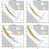Fig. 4 Similar to Fig. 3. Confidence regions with xpct5 and xcut5. Both upper panels are drawn with xpct5 and both lower panels with xcut5. Both left panels are the comparison between Lcg and Lsvg, and both right panels between Lsvg and Lvg.

From Sklar’s theorem (Sklar 1959), any multivariate distribution P(x₁,...,x_d) can be decomposed into the copula density multiplied by marginalized distributions. A comprehensible and elegant demonstration is given by Rüchendorf (2009). Readers are also encouraged to follow Scherrer et al. (2010) for detailed physical interpretations and Sato et al. (2011) for a very pedagogical derivation of the Gaussian copula transform.

Consider a d-dimensional distribution P(x), where x = (x₁,...,x_d) is a random vector. We let P_i be the marginalized 1-point PDF of x_i, and F_i the corresponding CDF. Sklar’s theorem shows that there is a unique d-dimensional function c defined on [ 0,1 ] ^d with uniform marginal PDF, such that $\begin{array}{ccc}\mathit{P}\mathrm{\left(}{x}\mathrm{\right)}\mathrm{=}\mathit{c}\mathrm{\left(}{u}\mathrm{\right)}{\mathit{P}}_{\mathrm{1}}\mathrm{\left(}{\mathit{x}}_{\mathrm{1}}\mathrm{\right)}\mathrm{·}\mathrm{·}\mathrm{·}{\mathit{P}}_{\mathit{d}}\mathrm{\left(}{\mathit{x}}_{\mathit{d}}\mathrm{\right)}\mathit{,}& & \end{array}$(11)where u_i ≡ F_i(x_i). The function c is called the copula density. On the other hand, let ${\mathit{q}}_{\mathit{i}}\mathrm{\equiv }{\mathrm{\Phi }}_{\mathit{i}}^{-1}\mathrm{\left(}{\mathit{u}}_{\mathit{i}}\mathrm{\right)}$, where Φ_i is the CDF of the normal distribution with the same means μ_i and variances ${\mathit{\sigma }}_{\mathit{i}}^{\mathrm{2}}$ as the laws P_i, such that $\begin{array}{ccc}{\mathrm{\Phi }}_{\mathit{i}}\mathrm{\left(}{\mathit{q}}_{\mathit{i}}\mathrm{\right)}& & \mathrm{\equiv }{\mathrm{\int }}_{\mathrm{-}\mathrm{\infty }}^{{\mathit{q}}_{\mathit{i}}}{\mathit{\phi }}_{\mathit{i}}\mathrm{\left(}{\mathit{q}}^{\mathrm{\prime }}\mathrm{\right)}\mathrm{d}{\mathit{q}}^{\mathrm{\prime }}\mathit{,}\\ {\mathit{\phi }}_{\mathit{i}}\mathrm{\left(}{\mathit{q}}_{\mathit{i}}\mathrm{\right)}& & \mathrm{\equiv }\frac{\mathrm{1}}{\sqrt{\mathrm{2}\mathit{\pi }{\mathit{\sigma }}_{\mathit{i}}^{\mathrm{2}}}}\exp \left[\mathrm{-}\frac{\mathrm{(}{\mathit{q}}_{\mathit{i}}\mathrm{-}{\mathit{\mu }}_{\mathit{i}}{\mathrm{)}}^{\mathrm{2}}}{\mathrm{2}{\mathit{\sigma }}_{\mathit{i}}^{\mathrm{2}}}\right]\mathrm{·}\end{array}$We can then define a new joint PDF P′ in the q space that corresponds to P in x space, i.e. P′(q) = P(x). The marginal PDF and CDF of P′ are only φ_i and Φ_i, respectively. Thus, applying Eq. (11) to P′ and φ_i leads to $\begin{array}{ccc}{\mathit{P}}^{\mathrm{\prime }}\mathrm{\left(}{q}\mathrm{\right)}\mathrm{=}\mathit{c}\mathrm{\left(}{u}\mathrm{\right)}{\mathit{\phi }}_{\mathrm{1}}\mathrm{\left(}{\mathit{q}}_{\mathrm{1}}\mathrm{\right)}\mathrm{·}\mathrm{·}\mathrm{·}{\mathit{\phi }}_{\mathit{d}}\mathrm{\left(}{\mathit{q}}_{\mathit{d}}\mathrm{\right)}\mathit{.}& & \end{array}$(14)By the uniqueness of the copula density, c in Eqs. (11)and (14)are the same. Thus, we obtain $\begin{array}{ccc}\mathit{P}\mathrm{\left(}{x}\mathrm{\right)}\mathrm{=}{\mathit{P}}^{\mathrm{\prime }}\mathrm{\left(}{q}\mathrm{\right)}\frac{{\mathit{P}}_{\mathrm{1}}\mathrm{\left(}{\mathit{x}}_{\mathrm{1}}\mathrm{\right)}\mathrm{·}\mathrm{·}\mathrm{·}{\mathit{P}}_{\mathit{d}}\mathrm{\left(}{\mathit{x}}_{\mathit{d}}\mathrm{\right)}}{{\mathit{\phi }}_{\mathrm{1}}\mathrm{\left(}{\mathit{q}}_{\mathrm{1}}\mathrm{\right)}\mathrm{·}\mathrm{·}\mathrm{·}{\mathit{\phi }}_{\mathit{d}}\mathrm{\left(}{\mathit{q}}_{\mathit{d}}\mathrm{\right)}}\mathrm{·}& & \end{array}$(15)We note that the marginal PDFs of P′ are identical to a multivariate Gaussian distribution φ with mean μ and covariance C, where C is the covariance matrix of x. The PDF of φ is given by $\begin{array}{ccc}\mathit{\phi }\mathrm{\left(}{q}\mathrm{\right)}& & \mathrm{\equiv }\frac{\mathrm{1}}{\sqrt{\mathrm{(}\mathrm{2}\mathit{\pi }{\mathrm{)}}^{\mathit{d}}\det {C}}}\exp \left[\mathrm{-}\frac{\mathrm{1}}{\mathrm{2}}\sum _{\mathit{i,j}}\mathrm{(}{\mathit{q}}_{\mathit{i}}\mathrm{-}{\mathit{\mu }}_{\mathit{i}}\mathrm{)}{\mathit{C}}_{\mathit{ij}}^{-1}\mathrm{(}{\mathit{q}}_{\mathit{j}}\mathrm{-}{\mathit{\mu }}_{\mathit{j}}\mathrm{)}\right]\mathrm{·}\end{array}$(16)Finally, by approximating P′ to φ, one gets the Gaussian copula transform: $\begin{array}{ccc}\mathit{P}\mathrm{\left(}{x}\mathrm{\right)}\mathrm{=}\mathit{\phi }\mathrm{\left(}{q}\mathrm{\right)}\frac{{\mathit{P}}_{\mathrm{1}}\mathrm{\left(}{\mathit{x}}_{\mathrm{1}}\mathrm{\right)}\mathrm{·}\mathrm{·}\mathrm{·}{\mathit{P}}_{\mathit{d}}\mathrm{\left(}{\mathit{x}}_{\mathit{d}}\mathrm{\right)}}{{\mathit{\phi }}_{\mathrm{1}}\mathrm{\left(}{\mathit{q}}_{\mathrm{1}}\mathrm{\right)}\mathrm{·}\mathrm{·}\mathrm{·}{\mathit{\phi }}_{\mathit{d}}\mathrm{\left(}{\mathit{q}}_{\mathit{d}}\mathrm{\right)}}\mathrm{·}& & \end{array}$(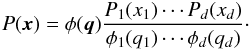17)Why is it more accurate to calculate the likelihood in this way? In the classical case, since the shape of P(x) is unknown, we approximate it to a normal distribution: P(x) ≈ φ(x). Applying the Gaussian copula transform means that we carry out this approximation in the new space of q: P′(q) ≈ φ(q). Since ${\mathit{q}}_{\mathit{i}}\mathrm{=}{\mathrm{\Phi }}_{\mathit{i}}^{-1}\mathrm{\left(}{\mathit{F}}_{\mathit{i}}\mathrm{\right(}{\mathit{x}}_{\mathit{i}}\mathrm{\left)}\mathrm{\right)}$, at least the marginals of P′(q) are strictly Gaussian. And Eq. (17) gives the corresponding value in x space, while taking P′(q) ≈ φ(q) in q space. However, in some cases, the copula has no effect at all. We consider f(x,y) = 2φ₂(x,y)Θ(xy) where φ₂ is the two-dimensional standard normal distribution, and Θ is the Heaviside step function. The value of f is two times φ₂ if x and y have the same sign and 0 otherwise. The marginal PDF of f and φ₂ turn out to be the same. As a result, the Gaussian copula transform does nothing and f remains extremely non-Gaussian. However, if we do not have any prior knowledge, then the result with the copula transformation should be at least as good as the classical likelihood.

By applying Eq. (17) to P(x^obs | π), one gets the copula likelihood: $\begin{array}{ccc}\mathrm{ℒ}\mathrm{\left(}{\pi }\mathrm{\right)}& \mathrm{=}& \frac{\mathrm{1}}{\sqrt{\mathrm{(}\mathrm{2}\mathit{\pi }{\mathrm{)}}^{\mathit{d}}\det {C}}}\\ & & \mathrm{\times }\exp \left[\mathrm{-}\frac{\mathrm{1}}{\mathrm{2}}\sum _{\mathit{i}\hspace{0.17em}\mathrm{=}\hspace{0.17em}\mathrm{1}}^{\mathit{d}}\sum _{\mathit{j}\mathrm{=}\mathrm{1}}^{\mathit{d}}\mathrm{(}{\mathit{q}}_{\mathit{i}}^{\mathrm{obs}}\mathrm{-}{\mathit{\mu }}_{\mathit{i}}\mathrm{)}{\mathit{C}}_{\mathit{ij}}^{-1}\mathrm{(}{\mathit{q}}_{\mathit{j}}^{\mathrm{obs}}\mathrm{-}{\mathit{\mu }}_{\mathit{j}}\mathrm{)}\right]\\ & & \\ & & \end{array}$(18)In this paper, ${\mathit{\mu }}_{\mathit{i}}\mathrm{=}{\mathit{x}}_{\mathit{i}}^{\mathrm{mod}}$. Including the dependency on π for all relevant quantities, the varying-covariance copula log-likelihood L_vc is given by $\begin{array}{ccc}{\mathit{L}}_{\mathrm{vc}}& \mathrm{\equiv }& \ln \left[\begin{array}{c}\det \end{array}\begin{array}{c}\mathrm{􏽢}\\ {C}\end{array}\mathrm{\left(}{\pi }\mathrm{\right)}\right]\\ & & \mathrm{+}\sum _{\mathit{i}\hspace{0.17em}\mathrm{=}\hspace{0.17em}\mathrm{1}}^{\mathit{d}}\sum _{\mathit{j}\mathrm{=}\mathrm{1}}^{\mathit{d}}\mathrm{(}{\mathit{q}}_{\mathit{i}}^{\mathrm{obs}}\mathrm{\left(}{\pi }\mathrm{\right)}\mathrm{-}{\mathit{x}}_{\mathit{i}}^{\mathrm{mod}}\mathrm{(}{\pi }{\mathrm{)}}^{\mathrm{)}}\begin{array}{c}\mathrm{􏽤}\\ {\mathit{C}}_{\mathit{ij}}^{-1}\end{array}\mathrm{\left(}{\pi }\mathrm{\right)}\mathrm{(}{\mathit{q}}_{\mathit{j}}^{\mathrm{obs}}\mathrm{\left(}{\pi }\mathrm{\right)}\mathrm{-}{\mathit{x}}_{\mathit{j}}^{\mathrm{mod}}\mathrm{(}{\pi }{\mathrm{)}}^{\mathrm{)}}\\ & & \mathrm{-}\mathrm{2}\sum _{\mathit{i}\hspace{0.17em}\mathrm{=}\hspace{0.17em}\mathrm{1}}^{\mathit{d}}\ln \mathit{\sigma ̂}\mathit{i}\mathrm{\left(}{\pi }\mathrm{\right)}\mathrm{-}\sum _{\mathit{i}\hspace{0.17em}\mathrm{=}\hspace{0.17em}\mathrm{1}}^{\mathit{d}}{\left(\frac{{\mathit{q}}_{\mathit{i}}^{\mathrm{obs}}\mathrm{\left(}{\pi }\mathrm{\right)}\mathrm{-}{\mathit{x}}_{\mathit{i}}^{\mathrm{mod}}\mathrm{\left(}{\pi }\mathrm{\right)}}{\mathit{\sigma ̂}\mathit{i}\mathrm{\left(}{\pi }\mathrm{\right)}}\right)}^{\mathrm{2}}\\ & & \end{array}$(19)Here, is the ith marginal π-dependent PDF that we estimate directly from the N samples ${\mathit{x}}_{\mathit{i}}^{\mathrm{\left(}\mathit{k}\mathrm{\right)}}\mathit{,k}\mathrm{=}\mathrm{1...}\mathit{N}$ already mentioned in Sect. 2.2, using the kernel density estimation (KDE): 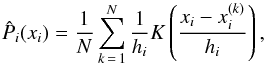$\begin{array}{ccc}\mathit{P̂}\mathit{i}\mathrm{\left(}{\mathit{x}}_{\mathit{i}}\mathrm{\right)}\mathrm{=}\frac{\mathrm{1}}{\mathit{N}}\sum _{\mathit{k}\hspace{0.17em}\mathrm{=}\hspace{0.17em}\mathrm{1}}^{\mathit{N}}\frac{\mathrm{1}}{{\mathit{h}}_{\mathit{i}}}\mathit{K}\left(\frac{{\mathit{x}}_{\mathit{i}}\mathrm{-}{\mathit{x}}_{\mathit{i}}^{\mathrm{\left(}\mathit{k}\mathrm{\right)}}}{{\mathit{h}}_{\mathit{i}}}\right)\mathit{,}& & \end{array}$(20)where the kernel K is Gaussian, and the bandwidth is given by Silverman’s rule (Silverman 1986). These are one-dimensional PDF estimations, and the time cost is almost negligible. The term $\mathit{P̂}{}_{\mathit{i}}\mathrm{\left(}{\mathit{x}}_{\mathit{i}}^{\mathrm{obs}}\mathrm{\right|}{\pi }\mathrm{)}$ should be understood as a one-point evaluation of this function at ${\mathit{x}}_{\mathit{i}}^{\mathrm{obs}}$. The quantities ${\mathit{x}}_{\mathit{i}}^{\mathrm{mod}}\mathrm{\left(}{\pi }\mathrm{\right)}$, , and $\begin{array}{c}{}_{\mathrm{􏽤}}\\ {\mathit{C}}_{\mathit{ij}}^{-1}\end{array}\mathrm{\left(}{\pi }\mathrm{\right)}$ are estimated with the same set following Eqs. (1)–(3). Finally, 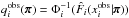${\mathit{q}}_{\mathit{i}}^{\mathrm{obs}}\mathrm{\left(}{\pi }\mathrm{\right)}\mathrm{=}{\mathrm{\Phi }}_{\mathit{i}}^{-1}\mathrm{\left(}\mathit{F̂}{}_{\mathit{i}}\mathrm{\right(}{\mathit{x}}_{\mathit{i}}^{\mathrm{obs}}\mathrm{\left|}{\pi }\mathrm{\right)}\mathrm{)}$. We highlight that is the CDF that corresponds to , and Φ_i also depends on π via μ_i and .

We are also interested in studying the copula transform under the constant-covariance situation. In this case, we define the constant-covariance copula log likelihood L_cc as 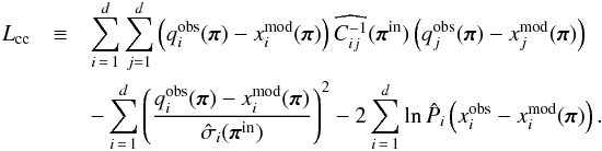$\begin{array}{ccc}{\mathit{L}}_{\mathrm{cc}}& \mathrm{\equiv }& \sum _{\mathit{i}\hspace{0.17em}\mathrm{=}\hspace{0.17em}\mathrm{1}}^{\mathit{d}}\sum _{\mathit{j}\mathrm{=}\mathrm{1}}^{\mathit{d}}\mathrm{(}{\mathit{q}}_{\mathit{i}}^{\mathrm{obs}}\mathrm{\left(}{\pi }\mathrm{\right)}\mathrm{-}{\mathit{x}}_{\mathit{i}}^{\mathrm{mod}}\mathrm{(}{\pi }{\mathrm{)}}^{\mathrm{)}}\begin{array}{c}\mathrm{􏽤}\\ {\mathit{C}}_{\mathit{ij}}^{-1}\end{array}\mathrm{\left(}{{\pi }}^{\mathrm{in}}\mathrm{\right)}\mathrm{(}{\mathit{q}}_{\mathit{j}}^{\mathrm{obs}}\mathrm{\left(}{\pi }\mathrm{\right)}\mathrm{-}{\mathit{x}}_{\mathit{j}}^{\mathrm{mod}}\mathrm{(}{\pi }{\mathrm{)}}^{\mathrm{)}}\\ & & \\ & & \end{array}$(21)Besides the constant covariance, we also suppose that the distribution of each x_i around its mean value does not vary with π. In this case, denotes the zero-mean marginal PDF, and it is only estimated once from the 1000 realizations of πⁱⁿ, as are and $\begin{array}{c}{\mathrm{􏽤}}_{}\\ {\mathit{C}}_{\mathit{ij}}^{-1}\end{array}$. We recall that 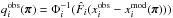${\mathit{q}}_{\mathit{i}}^{\mathrm{obs}}\mathrm{\left(}{\pi }\mathrm{\right)}\mathrm{=}{\mathrm{\Phi }}_{\mathit{i}}^{-1}\mathrm{\left(}\mathit{F̂}{}_{\mathit{i}}\mathrm{\right(}{\mathit{x}}_{\mathit{i}}^{\mathrm{obs}}\mathrm{-}{\mathit{x}}_{\mathit{i}}^{\mathrm{mod}}\mathrm{\left(}{\pi }\mathrm{\right)}\mathrm{\left)}\mathrm{\right)}$ where Φ_i depends on π implicitly via μ_i and .

4.2. Constraints using the copula

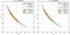Fig. 5 Confidence regions derived from copula analyses. Left panel: comparison between contours from Lcg (solid and dashed lines) and Lcc (colored areas). Right panel: comparison between contours from Lcc (colored areas) and Lvc (solid and dashed lines). The evolution tendency from Lcc to Lvc is similar to the evolution from Lcg to Lvg.

We again use the setting described in Sect. 2.2. We outline two interesting comparisons, which are shown in Fig. 5: between L_cg and L_cc in the lefthand panel and between L_cc and L_vc in the righthand one, both with x^abd5. The lefthand panel shows that, for weak-lensing peak counts, the Gaussian likelihood is a very good approximation. Quantitative results, shown in Tables 4–7, reveal that the Gaussian likelihood provides slightly optimistic Ω_m-σ₈ constraints. We would like to emphasize that the effect of the copula transform is ambiguous, and both tighter or wider constraints are possible. This has already shown by Sato et al. (2011), who found that the Gaussian likelihood underestimates the constraint power for low ℓ of the lensing power spectrum and overestimates it for high ℓ.

In the righthand panel of Fig. 5, when the CDC effect is taken into account for the copula transform, the parameter constrains are submitted to a similar change to the Gaussian likelihood. Tighter constraints are obtained from L_vc than from L_cc. Similar results can be found for x^pct5 and x^cut5. In summary, the copula with varying covariance, L_vc results in an FoM improvement of at least 10% compared to the Gaussian case with constant covariance, L_cg.

5. Non-analytic likelihood analyses

5.1. The true likelihood

In this section, we obtain the parameter constraints in a more direct way. Since our model predictions sample the full PDF, the PDF-Gaussianity assumption is no longer necessary. This allows us to go back to the true definition of the log-likelihood: 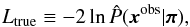$\begin{array}{ccc}{\mathit{L}}_{\mathrm{true}}\mathrm{\equiv }\mathrm{-}\mathrm{2}\ln \mathit{P̂}\mathrm{\left(}{{x}}^{\mathrm{obs}}\mathrm{\right|}{\pi }\mathrm{)}\mathit{,}& & \end{array}$(22)where is estimated from our N realizations x^(k) (π-dependent) using the kernel density estimation technique. The multivariate estimation is performed by $\begin{array}{ccc}\mathit{P̂}\mathrm{\left(}{x}\mathrm{\right)}& \mathrm{=}& \frac{\mathrm{1}}{\mathit{N}}\sum _{\mathit{k}\hspace{0.17em}\mathrm{=}\hspace{0.17em}\mathrm{1}}^{\mathit{N}}\mathit{K}\mathrm{(}{x}\mathrm{-}{{x}}^{\mathrm{\left(}\mathit{k}\mathrm{\right)}}\mathrm{)}\mathit{,}\\ \mathit{K}\mathrm{\left(}{x}\mathrm{\right)}& \mathrm{=}& \frac{\mathrm{1}}{\sqrt{\mathrm{\left(}\mathrm{2}\mathit{\pi }{\mathrm{)}}^{\mathit{d}}\mathrm{\right|}\det {H}\mathrm{|}}}\exp \left[\mathrm{-}\frac{\mathrm{1}}{\mathrm{2}}{{x}}^{\mathit{T}}{{H}}^{-1}{x}\right]\mathit{,}\end{array}$where $\begin{array}{ccc}\sqrt{{{H}}_{\mathit{ij}}}\mathrm{=}\{\begin{array}{c}\\ & & \\ & & \end{array}& & \end{array}$(25)The evaluation of this non-analytic likelihood gets very noisy when the observable dimension d increases. In this case, a larger N will be required to stabilize the constraints. As in previous sections, we perform both the likelihood-ratio test and Bayesian inference with this likelihood.

5.2. p-value analysis

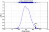Fig. 6 Example for the p-value determination. The x-axis indicates a one-dimensional observable, and the y-axis is the PDF. The PDF is obtained from a kernel density estimation using the N = 1000 realizations. Their values are shown as bars in the rug plot at the top of the panel. The shaded area is the corresponding p-value for given observational data xobs.

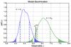Fig. 7 PDF from two different models (denoted by π1 and π2) and the observation xobs. The dashed lines show 1σ intervals for both models, while the shaded areas are intervals beyond the 2σ level. In this figure, model π1 is excluded at more than 2σ, whereas the significance of the model π2 is between 1 and 2σ.

Another non-analytic technique is the p-value analysis. This frequentist approach provides the significance level by directly determining the p-value associated with a observation x^obs. The p-value is defined as 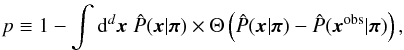$\begin{array}{ccc}\mathit{p}\mathrm{\equiv }\mathrm{1}\mathrm{-}\mathrm{\int }{\mathrm{d}}^{\mathit{d}}{x}\mathit{P̂}\mathrm{\left(}{x}\mathrm{\right|}{\pi }\mathrm{)}\mathrm{\times }\mathrm{\Theta }\mathrm{(}\mathit{P̂}\mathrm{\left(}{x}\mathrm{\right|}{\pi }\mathrm{)}\mathrm{-}\mathit{P̂}\mathrm{(}{{x}}^{\mathrm{obs}}\mathrm{|}{\pi }{\mathrm{)}}^{\mathrm{)}}\mathit{,}& & \end{array}$(26)where Θ denotes the Heaviside step function. The integral extends over the region where x is more probable than x^obs for a given π, as shown by Fig. 6. Thus, the interpretation of Eq. (26) is that if we generated N universes, then at least (1 − p)N of them should have an observational result “better” than x^obs. In this context, “better” refers to a more probable realization. The significance level is determined by the chi-squared distribution with d = 2 deg of freedom, for two free parameters, Ω_m and σ₈. As Fig. 7 shows, this provides a straightforward way to distinguish different cosmological models.

As in Sect. 4.2, we used KDE to estimate the multivariate PDF and numerically integrated Eq. (26) to obtain the p-value. Monte Carlo integration is used for evaluating the five-dimensional integrals.

5.3. Parameter constraints

Figure 8 shows the confidence contours from L_true and p-value analysis with observables x^abd5. We notice that these constraints are very noisy. This is due to a relatively low number of realizations to estimate the probability and prevents us from making definite conclusions. Nevertheless, the result from the lefthand panel reveals good agreement between constraints from two likelihoods. This suggests that we may substitute L_true with the CDC-copula likelihood to bypass the drawback of noisy estimation from L_true. In the righthand panel, the result from p-value analysis seems to be larger. We reduced the noise for the p-value analysis by combining x^abd5 into a two-component vector. In this case, the p-value is evaluated using the grid integration. This data compression technique does not significantly enlarge but visibly smooths the contours.

In the L_true case, the probability information that we need is local since the likelihood P is only evaluated at x^obs. For p-value analysis, one needs to determine the region where P(x) <P(x^obs) and integrate over it, so a more global knowledge of P(x) is needed in this case. We recall that KDE smooths, thus the estimation is always biased (Zambom & Dias 2012). Other estimations, for example using the Voronoi-Delaunay tessellation (see, e.g., Schaap 2007; Guio & Achilleos 2009), could be an alternative to the KDE technique. As a result, observable choice, data compression, and density estimation need to be considered jointly for all non-analytic approaches.

Recent results from CFHTLenS (LPH15) and Stripe-82 (LPL15) resulted in ΔΣ₈ ~ 0.1, about 2–3 times larger than this study. However, we would like to highlight that redshift errors are not taken into account here and that the simulated galaxy density used in this work is much higher. Also, we choose z_s = 1, which is higher than the median redshift of both surveys (~0.75). All these factors contribute to our smaller error bars.

6. Approximate Bayesian computation

6.1. PMC ABC algorithm

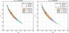Fig. 8 Left panel: confidence regions derived from Lvc (colored areas) and Ltrue (solid and dashed lines) with xabd5. Right panel: confidence regions derived from Lvc (colored areas) and p-value analysis (solid and dashed lines). The contours from Ltrue and p-value analysis are noisy due to a relatively low N for probability estimation. We notice that Lvc and Ltrue yield very similar results.

In the previous section, we presented parameter constraints derived from directly evaluating the underlying PDF. Now, we want to move a step further and bypass the likelihood estimation altogether.

Based on an accept-reject rule, approximate Bayesian computation (ABC) is an algorithm that provides an approximate posterior distribution of a complex stochastic process when evaluating the likelihood is expensive or unreachable. There are only two requirements: (1) a stochastic model for the observed data that samples the likelihood function of the observable; and (2) a measure, called summary statistic, to perform model comparison. We present below a brief description of ABC. Readers can find detailed reviews of ABC in Marin et al. (2011) and Sect. 1 of Cameron & Pettitt (2012).

The idea behind ABC can be most easily illustrated in the case of discrete data as follows. Instead of explicitly calculating the likelihood, one first generates a set of parameters { π_i } as samples under the prior , and then for each π_i simulates a model prediction X sampled under the likelihood function P(· | π_i). (Here we put X in the upper case to emphasize that X is a random variable.) Keeping only those π_i for which X = x^obs, the distribution of the accepted samples equals the posterior distribution of the parameter given the observed data, since $\begin{array}{ccc}{\mathrm{𝒫}}_{\mathrm{ABC}}\mathrm{\left(}{\pi }\mathrm{\right)}& \mathrm{=}& \sum _{{X}}\mathit{P}\mathrm{\left(}{X}\mathrm{\right|}{\pi }\mathrm{\left)}\mathrm{𝒫}\mathrm{\right(}{\pi }\mathrm{)}{\mathit{\delta }}_{{X}\mathit{,}{{x}}^{\mathrm{obs}}}\\ & \mathrm{=}& \mathit{P}\mathrm{(}{{x}}^{\mathrm{obs}}\mathrm{|}{{\pi }}^{\mathrm{)}}\mathrm{𝒫}\mathrm{\left(}{\pi }\mathrm{\right)}\\ & \mathrm{=}& \end{array}$(27)where δ_X,x^obs is Kronecker’s delta. Therefore, { π_i } is an independent and identically distributed sample from the posterior. It is sufficient to perform a one-sample test: using a single realization X for each parameter π to obtain a sample under the posterior.

ABC can also be adapted to continuous data and parameters, where obtaining a strict equality X = x^obs is pratically impossible. As a result, sampled points are accepted with a tolerance levelϵ, say | X − x^obs | ≤ ϵ. What is retained after repeating this process is an ensemble of parameters π that are compatible with the data and that follow a probability distribution, which is a modified version of Eq. (27), $\begin{array}{ccc}{\mathrm{𝒫}}_{\mathit{ϵ}}\mathrm{\left(}{\pi }\mathrm{\right|}{{x}}^{\mathrm{obs}}\mathrm{)}\mathrm{=}{\mathit{A}}_{\mathit{ϵ}}\mathrm{(}{\pi }\mathrm{\left)}\mathrm{𝒫}\mathrm{\right(}{\pi }\mathrm{)}\mathit{,}& & \end{array}$(28)where A_ϵ(π) is the probability that a proposed parameter π passes the one-sample test within the error ϵ: $\begin{array}{ccc}{\mathit{A}}_{\mathit{ϵ}}\mathrm{\left(}{\pi }\mathrm{\right)}\mathrm{\equiv }\mathrm{\int }\mathrm{d}{X}\mathit{P}\mathrm{\left(}{X}\mathrm{\right|}{\pi }\mathrm{\left)}{{1}}_{\mathrm{|}{X}\mathrm{-}{{x}}^{\mathrm{obs}}\mathrm{|}\mathrm{\le }\mathit{ϵ}}\mathrm{\right(}{X}\mathrm{)}\mathit{.}& & \end{array}$(29)The Kronecker delta from Eq. (27) has now been replaced with the indicator function of the set of points X that satisfy the tolerance criterion. The basic assumption of ABC is that the probability distribution (28) is a good approximation of the underlying posterior, such that ${\mathrm{𝒫}}_{\mathit{ϵ}}\mathrm{\left(}{\pi }\mathrm{\right|}{{x}}^{\mathrm{obs}}\mathrm{)}\mathrm{\approx }\mathrm{𝒫}\mathrm{(}{\pi }\mathrm{\left|}{{x}}^{\mathrm{obs}}\mathrm{\right)}\mathit{.}$(30)Therefore, the error can be seperated into two parts: one from the approximation above and the other from the estimation of the desired integral, . For the latter, gathering one-sample tests of A_ϵ makes a Monte Carlo estimation of , which is unbiased. This ensures the use of the one-sample test.

A further addition to the ABC algorithm is a reduction in the complexity of the full model and data. This is necessary in cases of very large dimensions, for example, when the model produces entire maps or large catalogs. The reduction of data complexity is done with the so-called summary statistic s. For instance, in our peak-count framework, a complete data set x is a peak catalog with positions and S/N values, and the summary statistic s is chosen here to be s(x) = x^abd5, x^pct5, or x^cut5, respectively, for the three cases of observables introduced in Sect. 2.2. As a remark, if this summary statistic is indeed sufficient, then Eq. (30) will no longer be an approximation. The true posterior can be recovered when ϵ → 0.

For a general comparison of model and data, one chooses a metric D adapted to the summary statistic s, and the schematic expression | X − x^obs | ≤ ϵ used above is generalized to D(s(X),s(x^obs)) ≤ ϵ. We highlight that the summary statistic can have a low dimension and a very simple form. In practice, it is motivated by computational efficiency, and it seems that a simple summary can still produce reliable constraints (Weyant et al. 2013).

The integral of Eq. (28) over π is smaller than unity, and the deficit only represents the probability that a parameter is rejected by ABC. This is not problematic since density estimation will automatically normalize the total integral over the posterior. However, a more subtle issue is the choice of the tolerance level ϵ. If ϵ is too high, A(π) is close to 1, and Eq. (30) becomes a bad estimate. If ϵ is too low, A(π) is close to 0, and sampling becomes extremely difficult and inefficient. How, then, should one choose ϵ? This can be done by applying the iterative importance sampling approach of population Monte Carlo (PMC; for applications to cosmology, see Wraith et al. 2009) and combine it with ABC (Del Moral et al. 2006; Sisson et al. 2007). This joint approach is sometimes called SMC ABC, where SMC stands for sequential Monte Carlo; we refer to it as PMC ABC. The idea of PMC ABC is to iteratively reduce the tolerance ϵ until a stopping criterion is reached.

Algorithm 8 details the steps for PMC ABC. We let be a probabilistic model for x given π. PMC ABC requires a prior ρ(π), a summary statistic s(x) that retains only partial information about x, a distance function D based on the dimension of s(x), and a shutoff parameter r_stop. We denote as a multivariate normal with mean π and covariance matrix C, K(π,C) ∝ exp(−π^TC^-1π/2) a Gaussian kernel, the weighted covariance for the set { π₁,...,π_p } with weights { w₁,...,w_p }, and p the number of particles, i.e., the number of sample points in the parameter space.

In the initial step, PMC ABC accepts all particles drawn from the prior and defines an acceptance tolerance before starting the first iteration. The tolerance is given by the median of the distances of the summary statistic between the observation and the stochastic model generated from each particle. Then, each iteration is carried out by an importance-sampling step based on weights determined by the previous iteration. To find a new particle, a previous point ${{\pi }}_{\mathit{j}}^{\mathrm{(}\mathit{t}\mathrm{-}\mathrm{1}\mathrm{)}}$ is selected according to its weight. A candidate particle is drawn from a proposal distribution, which is a normal law centered on ${{\pi }}_{\mathit{j}}^{\mathrm{(}\mathit{t}\mathrm{-}\mathrm{1}\mathrm{)}}$ with a covariance equal to the covariance of all particles from the previous iteration. With a model generated using the candidate particle, we accept the new particle if the distance between the model and the observation is shorter than the tolerance, and reject it otherwise. After accepting p particles, the success rate, defined as the ratio of accepted particles to total tries, is updated. The iterations continue until the success rate decreases below the shutoff value. Instead of defining a minimal tolerance (Beaumont et al. 2002; Fearnhead & Prangle 2010; Weyant et al. 2013), we use a simplified stopping criterion that is based on the selection efficiency of the algorithm. Since McKinley et al. (2009) prove that the stopping criterion has very little impact on the estimated posterior, the choice of the tolerance level is instead a question of computational power.

6.2. Settings for ABC

McKinley et al. (2009) studied the impact of the various choices necessary for ABC, by comparing Markov chain Monte Carlo (MCMC) ABC and PMC ABC. The authors concluded that (1) increasing the number of simulations beyond one for a given parameter does not seem to improve the posterior estimation (similar conclusion found by Bornn et al. 2014); (2) the specific choice of the tolerance level does not seem to be important; (3) the choice of the summary statistic and the distance is crucial; and (4) PMC ABC performs better than MCMC ABC. Therefore, exploring a sufficient summary statistic to represent the whole data set becomes an essential concern for the ABC technique.

To solve the optimal data compression problem, Blum et al. (2013) provide a series of methods in their review for selecting the ideal summaries, as well as methods of reducing the data dimension. Leaving a detailed study of optimal choice for the future work, we adopted a straightforward summary statistic in this work, defined as s(x) = x^type5, and the distance as $\begin{array}{ccc}\mathit{D}\mathrm{\left(}{{x}}^{\mathrm{type}\mathrm{5}}\mathit{,}{{y}}^{\mathrm{type}\mathrm{5}}\mathrm{\right)}\mathrm{=}\sqrt{\sum _{\mathit{i}\hspace{0.17em}\mathrm{=}\hspace{0.17em}\mathrm{1}}^{\mathrm{5}}\frac{{\mathrm{(}{\mathit{x}}_{\mathit{i}}^{\mathrm{type}\mathrm{5}}\mathrm{-}{{\mathit{y}}_{\mathit{i}}^{\mathrm{type}\mathrm{5}}}^{\mathrm{)}}}^{\mathrm{2}}}{{\mathit{C}}_{\mathit{ii}}}}\mathrm{·}& & \end{array}$(31)This is simply a weighted Euclidean distance, where the weight ${\mathit{C}}_{\mathit{ii}}^{-1}$ is needed to level out the values of the different S/N.

The prior ρ is chosen to be flat. We set p = 250 and r_stop = 0.02. In this condition, we can easily compare the computational cost with the analyses presented in previous sections. If τ is the time cost for one model realization, the total time consumption is 7821 × 1000 × τ for our likelihood-based analyses in Sects. 3–5, and $\mathrm{250}\mathrm{\times }\mathrm{1}\mathrm{\times }\mathrm{\left(}{\sum }_{\mathit{t}}{\mathit{r}}_{\mathit{t}}^{-1}\mathrm{\right)}\mathrm{\times }\mathit{\tau }$ for ABC where r_t is the acceptance rate of the t-th iteration. For x^abd5, ${\sum }_{\mathit{t}}{\mathit{r}}_{\mathit{t}}^{-1}\mathrm{\approx }\mathrm{102}$ (0 ≤ t ≤ 9), so the computation time for ABC is drastically reduced by a factor of ~300 compared to the likelihood analyses. ABC is faster by a similar factor compared to Monte-Carlo sampling, since typically the number of required sample points is , the same order of magnitude as our number of grid points.

6.3. Results from ABC

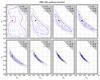Fig. 9 Evolution of particles and the posterior from the PMC ABC algorithm. We show results from the first 8 iterations (0 ≤ t ≤ 7). Particles are given by blue dots. Solid lines are 1σ contours, and dashed lines are 2σ contours. White areas represent the prior. The corresponding accept rate r and tolerance level ϵ are also given. We set ϵ(0) = +∞.

Figure 9 shows the iterative evolution of the PMC ABC particles. We drew the position of all 250 particles and credible regions for the first eight iterations. The summary statistic is x^abd5. The credible regions were drawn from the posterior estimated on a grid using KDE with the ABC particles as sample points x^(k) in Eq. (23). We ignored the particle weights for this density estimate. We find that the contours stablize for t ≥ 8, which correponds to an acceptance rate of r = 0.05. At these low accpetence rates, corresponding to a small tolerance, the probability of satisfying the tolerance criterion D(s(X),s(x^obs)) ≤ ϵ is low even though X is sampled from parameters in the high-probability region, and accepting a proposed particle depends mainly on random fluctuations due to the stochasticity of the model.

In Fig. 10, we show the weights of particles sampled at the final iteration t = 8. The weight is visualized by both color and size of the circle. The figure shows that points farther away from the maximum have larger weights as constructed by Algorithm 8. Since those points are more isolated, their weights compensate for the low density of points, avoiding undersampling the tails of the posterior and overestimating the constraining power.

In Fig. 11 we show the comparison of credible regions between L_cg and PMC ABC with s(x) = x^abd5. The FoM and the best-fit ABC results are presented in Tables 6 and 7, respectively. The figure shows good agreement between the two cases, and thus validates the performance of PMC ABC. The broader contours from ABC might be caused by a bias of KDE. The same reason might be responsible for the slight shift of the contours in the tails of the distribution, which do not follow the particles exactly, which are best visible in the two lefthand panels in the lower row of Fig. 9.

7. Summary and discussion

Our model for weak-lensing peak counts, which provides a direct estimation of the underlying PDF of observables, leads to a wide range of possibilities for constraining parameters. To summarize this work, we

• compared different data vector choices;

• studied the dependence of the likelihood on cosmology;

• explored the full PDF information of observables;

• proposed different constraint strategies; and

• examined them with two criteria.

In this paper, we performed three different series of analyses – the Gaussian likelihood, the copula likelihood, and non-analytic analyses – by using three different data vectors: one based on the peak PDF and two on the CDF. We defined two quantitative criteria: ΔΣ₈, which represents the error bar on the parameter Σ₈ = σ₈(Ω_m/ 0.27)^α and is a measure of the width of the Ω_m-σ₈ degeneracy direction; and FoM, which is the area of the Ω_m-σ₈ contour. Both Bayesian and frequentist approaches were followed. Although the interpretations are different, the results are very similar.

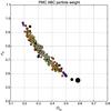Fig. 10 Weights of particles from t = 8 with s(x) = xabd5. The weight is represented by the size and the color at the same time.

Fig. 11 Comparison between credible regions derived from Lcg (colored areas) and ABC (solid and dashed lines).

We studied the cosmology-dependent-covariance (CDC) effect by estimating the true covariance for each parameter set. We found that the CDC effect can increase the constraining power up to 22%. The main contribution comes from the additional variation of the χ² term, and the contribution from the determinant term is negligible. These observations confirm a previous study by Eifler et al. (2009).

We also performed a copula analysis, which makes weaker assumptions than Gaussianity. In this case, the marginalized PDF is Gaussianized by the copula transform. The result shows that the difference with the Gaussian likelihood is small. This is dominated by the CDC effect if a varying covariance is taken into account.

Discarding the Gaussian hypothesis on the PDF of observables, we provided two straightforward ways of using the full PDF information. The first one is the true likelihood. The direct evaluation of the likelihood is noisy owing to the high statistical fluctuations from the finite number of sample points. However, we find that the varying-covariance copula likelihood, noted as L_vc above, seems to be a good approximation to the truth. The second method is to determine the p-value for a given parameter set directly, and this approach gives us more conservative constraints. We outline that both methods are covariance-free, avoiding non-linear effects caused by the covariance inversion.

At the end we showed how approximate Bayesian computation (ABC) derives cosmological constraints using the accept-reject sampling. Combined with importance sampling, this method requires less computational resources than all the others. We proved that by reducing the computational time by a factor of 300, ABC is able to yield consistent constraints from weak-lensing peak counts. Furthermore, Weyant et al. (2013) show in their study that ABC is able to perform unbiased constraints using contaminated data, demonstrating the robustness of this algorithm.

A comparison between different data vectors is done in this study. Although we find for all analyses that x^abd5 outperforms x^pct5 by 20–40% in terms of FoM, this is not necessarily true in general when we use a different percentile choice. Actually, the performance of x^pct depends on the correlation between its different components. However, the x^pct family is not recommended in practice because of model biases induced for very low peaks (S/N< 0). In addition, our study shows that the x^cut family is largely outperformed by x^abd. Thus, we conclude that x^abd seems to be good candidates for peak-count analysis, while the change in the contour tilt from x^cut could be interesting when combining with other information.

The methodology that we show for parameter constraints can be applied to all fast stochastic forward models. Flexible and efficient, this approach possesses a great potential whenever the modeling of complex effects is desired. Our study displays two different parameter-constraint philosophies. On the one hand, parameteric estimation (Sects. 3 and 4), under some specific hypotheses such as Gaussianity, only requires some statistical quantities such as the covariances. However, the appropriateness of the likelihood should be examined and validated to avoid biases. On the other hand, non-analytic estimation (Sects. 5 and 6) is directly derived from the PDF. The problem of inappropriateness vanishes, but instead the uncertainty and bias of density estimation become drawbacks. Depending on modeling pertinence, an aspect may be more advantageous than another. Although not studied in this work, a hybrid approach using semi-analytic estimator could be interesting. This solicits more detailed studies of trade-off between the inappropriatenss of analytic estimators and the uncertainty of density estimation.

Acknowledgments

This work is supported by Région d’Île-de-France in the framework of a DIM-ACAV thesis fellowship. We also acknowledge the support from the French national program for cosmology and galaxies (PNCG). The authors wish to acknowledge the anonymous referee for reviewing the paper. Chieh-An Lin would like to thank Karim Benabed, Ewan Cameron, Yu-Yen Chang, Yen-Chi Chen, Cécile Chenot, François Lanusse, Sandrine Pires, Fred Ngolè, Florent Sureau, and Michael Vespe for useful discussions and suggestions on diverse subjects.

References

All Tables

All Figures

Fig. 1 Location of 7821 points on which we evaluate the likelihoods. In the condensed area, the interval between two grid points is 0.005, while in both wing zones it is 0.01. The black star shows $\mathrm{\left(}{\mathrm{\Omega }}_{\mathrm{m}}^{\mathrm{in}}\mathit{,}{\mathit{\sigma }}_{\mathrm{8}}^{\mathrm{in}}\mathrm{\right)}\mathrm{=}\mathrm{\left(}\mathrm{0.28}\mathit{,}\mathrm{0.82}\mathrm{\right)}$.

In the text

Fig. 2 Middle panel: likelihood value using xabd5 on the Ωm-Σ8 plane. The green star represents the input cosmology πin. Since log σ8 and log Ωm form an approximately linear degenerency, the quantity Σ8 ≡ σ8(Ωm/ 0.27)α allows us to characterize the banana-shape contour thickness. Right panel: the marginalized PDF of Σ8. The dashed lines give the 1σ interval (68.3%), while the borders of the shaded areas represent 2σ limits (95.4%). Left panel: log-value of the marginalized likelihood ratio. Dashed lines in the left panel give the corresponding value for 1 and 2σ significance levels, respectively.

In the text

Fig. 3 Confidence regions derived from Lcg, Lsvg, and Lvg with xabd5. The solid and dashed lines represent Lcg in the left panel and Lvg in the right panel, while the colored areas are from Lsvg. The black star stands for πin and gray areas represent the non-explored parameter space. The dotted lines are different isolines, the variance Ĉ55 of the bin with highest S/N in the left panel and ln(detĈ) for the right panel. The contour area is reduced by 22% when taking the CDC effect into account. The parameter-dependent determinant term does not contribute significantly.

In the text

	Fig. 4 Similar to Fig. 3. Confidence regions with xpct5 and xcut5. Both upper panels are drawn with xpct5 and both lower panels with xcut5. Both left panels are the comparison between Lcg and Lsvg, and both right panels between Lsvg and Lvg.
In the text

	Fig. 5 Confidence regions derived from copula analyses. Left panel: comparison between contours from Lcg (solid and dashed lines) and Lcc (colored areas). Right panel: comparison between contours from Lcc (colored areas) and Lvc (solid and dashed lines). The evolution tendency from Lcc to Lvc is similar to the evolution from Lcg to Lvg.
In the text

	Fig. 6 Example for the p-value determination. The x-axis indicates a one-dimensional observable, and the y-axis is the PDF. The PDF is obtained from a kernel density estimation using the N = 1000 realizations. Their values are shown as bars in the rug plot at the top of the panel. The shaded area is the corresponding p-value for given observational data xobs.
In the text

	Fig. 7 PDF from two different models (denoted by π1 and π2) and the observation xobs. The dashed lines show 1σ intervals for both models, while the shaded areas are intervals beyond the 2σ level. In this figure, model π1 is excluded at more than 2σ, whereas the significance of the model π2 is between 1 and 2σ.
In the text

	Fig. 8 Left panel: confidence regions derived from Lvc (colored areas) and Ltrue (solid and dashed lines) with xabd5. Right panel: confidence regions derived from Lvc (colored areas) and p-value analysis (solid and dashed lines). The contours from Ltrue and p-value analysis are noisy due to a relatively low N for probability estimation. We notice that Lvc and Ltrue yield very similar results.
In the text

	Fig. 9 Evolution of particles and the posterior from the PMC ABC algorithm. We show results from the first 8 iterations (0 ≤ t ≤ 7). Particles are given by blue dots. Solid lines are 1σ contours, and dashed lines are 2σ contours. White areas represent the prior. The corresponding accept rate r and tolerance level ϵ are also given. We set ϵ(0) = +∞.
In the text

	Fig. 10 Weights of particles from t = 8 with s(x) = xabd5. The weight is represented by the size and the color at the same time.
In the text

	Fig. 11 Comparison between credible regions derived from Lcg (colored areas) and ABC (solid and dashed lines).
In the text

References

- Akeret, J., Refregier, A., Amara, A., Seehars, S., & Hasner, C. 2015, JCAP, 08, 043 [CrossRef] [Google Scholar]
- Albrecht, A., Bernstein, G., Cahn, R., et al. 2006, ArXiv e-prints [arXiv:astro-ph/0609591] [Google Scholar]
- Bard, D., Kratochvil, J. M., Chang, C., et al. 2013, ApJ, 774, 49 [NASA ADS] [CrossRef] [Google Scholar]
- Beaumont, M. A., Zhang, W., & Balding, D. J. 2002, Genetics, 162, 2025 [Google Scholar]
- Beaumont, M. A., Cornuet, J.-M., Marin, J.-M., & Robert, C. P. 2009, Biometrika, 96, 983 [CrossRef] [Google Scholar]
- Benabed, K., Cardoso, J.-F., Prunet, S., & Hivon, E. 2009, MNRAS, 400, 219 [NASA ADS] [CrossRef] [Google Scholar]
- Bergé, J., Amara, A., & Réfrégier, A. 2010, ApJ, 712, 992 [NASA ADS] [CrossRef] [Google Scholar]
- Berger, J. O., Fienberg, S. E., Raftery, A. E., & Robert, C. P. 2010, Proc. National Academy Sci., 107, 157 [CrossRef] [Google Scholar]
- Blum, M. G. B., Nunes, M. A., Prangle, D., & Sisson, S. A. 2013, Statistical Science, 28, 189 [CrossRef] [Google Scholar]
- Bornn, L., Pillai, N., Smith, A., & Woodard, D. 2014, ArXiv e-prints [arXiv:1404.6298] [Google Scholar]
- Cameron, E., & Pettitt, A. N. 2012, MNRAS, 425, 44 [NASA ADS] [CrossRef] [Google Scholar]
- Casella, G., & Berger, R. L. 2002, Statistical Inference (Duxbury) [Google Scholar]
- Csilléry, K., Blum, M. G., Gaggiotti, O. E., & François, O. 2010, Trends in Ecology & Evolution, 25, 410 [Google Scholar]
- Del Moral, P., Doucet, A., & Jasra, A. 2006, J. Roy. Statist. Soc.: Series B (Statistical Methodology), 68, 411 [Google Scholar]
- Dietrich, J. P., & Hartlap, J. 2010, MNRAS, 402, 1049 [NASA ADS] [CrossRef] [Google Scholar]
- Drovandi, C. C., & Pettitt, A. N. 2011, Biometrics, 67, 225 [CrossRef] [Google Scholar]
- Eifler, T., Schneider, P., & Hartlap, J. 2009, A&A, 502, 721 [NASA ADS] [CrossRef] [EDP Sciences] [Google Scholar]
- Fan, Z., Shan, H., & Liu, J. 2010, ApJ, 719, 1408 (FSL10) [NASA ADS] [CrossRef] [Google Scholar]
- Fearnhead, P., & Prangle, D. 2010, ArXiv e-prints [arXiv:1004.1112] [Google Scholar]
- Fu, L., Kilbinger, M., Erben, T., et al. 2014, MNRAS, 441, 2725 [NASA ADS] [CrossRef] [Google Scholar]
- Guio, P., & Achilleos, N. 2009, MNRAS, 398, 1254 [NASA ADS] [CrossRef] [Google Scholar]
- Hamana, T., Takada, M., & Yoshida, N. 2004, MNRAS, 350, 893 [NASA ADS] [CrossRef] [Google Scholar]
- Hamana, T., Sakurai, J., Koike, M., & Miller, L. 2015, PASJ, 67, 34 [NASA ADS] [Google Scholar]
- Hartlap, J., Simon, P., & Schneider, P. 2007, A&A, 464, 399 [NASA ADS] [CrossRef] [EDP Sciences] [Google Scholar]
- Hennawi, J. F., & Spergel, D. N. 2005, ApJ, 624, 59 [NASA ADS] [CrossRef] [Google Scholar]
- Ishida, E. E. O., Vitenti, S. D. P., Penna-Lima, M., et al. 2015, Astron. Comput., 13, 1 [Google Scholar]
- Jain, B., & Seljak, U. 1997, ApJ, 484, 560 [NASA ADS] [CrossRef] [Google Scholar]
- Jain, B., & Van Waerbeke, L. 2000, ApJ, 530, L1 [NASA ADS] [CrossRef] [Google Scholar]
- Jee, M. J., Tyson, J. A., Schneider, M. D., et al. 2013, ApJ, 765, 74 [NASA ADS] [CrossRef] [Google Scholar]
- Jenkins, A., Frenk, C. S., White, S. D. M., et al. 2001, MNRAS, 321, 372 [NASA ADS] [CrossRef] [MathSciNet] [Google Scholar]
- Jiang, I.-G., Yeh, L.-C., Chang, Y.-C., & Hung, W.-L. 2009, AJ, 137, 329 [NASA ADS] [CrossRef] [Google Scholar]
- Kainulainen, K., & Marra, V. 2009, Phys. Rev. D, 80, 123020 [NASA ADS] [CrossRef] [Google Scholar]
- Kainulainen, K., & Marra, V. 2011a, Phys. Rev. D, 83, 023009 [NASA ADS] [CrossRef] [Google Scholar]
- Kainulainen, K., & Marra, V. 2011b, Phys. Rev. D, 84, 063004 [NASA ADS] [CrossRef] [Google Scholar]
- Kilbinger, M., & Schneider, P. 2005, A&A, 442, 69 [NASA ADS] [CrossRef] [EDP Sciences] [Google Scholar]
- Kilbinger, M., Fu, L., Heymans, C., et al. 2013, MNRAS, 430, 2200 [NASA ADS] [CrossRef] [Google Scholar]
- Killedar, M., Borgani, S., Fabjan, D., et al. 2015, MNRAS, submitted [arXiv:1507.05617] [Google Scholar]
- Kratochvil, J. M., Haiman, Z., & May, M. 2010, Phys. Rev. D, 81, 043519 [NASA ADS] [CrossRef] [Google Scholar]
- Kruse, G., & Schneider, P. 1999, MNRAS, 302, 821 [NASA ADS] [CrossRef] [Google Scholar]
- Lin, C.-A., & Kilbinger, M. 2015, A&A, 576, A24 (Paper I) [NASA ADS] [CrossRef] [EDP Sciences] [Google Scholar]
- Liu, J., Haiman, Z., Hui, L., Kratochvil, J. M., & May, M. 2014, Phys. Rev. D, 89, 023515 [NASA ADS] [CrossRef] [Google Scholar]
- Liu, J., Petri, A., Haiman, Z., et al. 2015, Phys. Rev. D, 91, 063507 (LPH15) [NASA ADS] [CrossRef] [Google Scholar]
- Liu, X., Wang, Q., Pan, C., & Fan, Z. 2014, ApJ, 784, 31 [NASA ADS] [CrossRef] [Google Scholar]
- Liu, X., Pan, C., Li, R., et al. 2015, MNRAS, 450, 2888 (LPL15) [NASA ADS] [CrossRef] [Google Scholar]
- Maoli, R., Van Waerbeke, L., Mellier, Y., et al. 2001, A&A, 368, 766 [NASA ADS] [CrossRef] [EDP Sciences] [Google Scholar]
- Marian, L., Smith, R. E., & Bernstein, G. M. 2010, ApJ, 709, 286 [NASA ADS] [CrossRef] [Google Scholar]
- Marian, L., Hilbert, S., Smith, R. E., Schneider, P., & Desjacques, V. 2011, ApJ, 728, L13 [NASA ADS] [CrossRef] [Google Scholar]
- Marian, L., Smith, R. E., Hilbert, S., & Schneider, P. 2012, MNRAS, 423, 1711 [NASA ADS] [CrossRef] [Google Scholar]
- Marian, L., Smith, R. E., Hilbert, S., & Schneider, P. 2013, MNRAS, 432, 1338 [NASA ADS] [CrossRef] [Google Scholar]
- Marin, J.-M., Pudlo, P., Robert, C. P., & Ryder, R. J. 2011, ArXiv e-prints [arXiv:1101.0955] [Google Scholar]
- Maturi, M., Angrick, C., Pace, F., & Bartelmann, M. 2010, A&A, 519, A23 [NASA ADS] [CrossRef] [EDP Sciences] [Google Scholar]
- Maturi, M., Fedeli, C., & Moscardini, L. 2011, MNRAS, 416, 2527 [NASA ADS] [CrossRef] [Google Scholar]
- McKinley, T., Cook, A. R., & Deardon, R. 2009, Int. J. Biostatistics, 5, A24 [CrossRef] [Google Scholar]
- Navarro, J. F., Frenk, C. S., & White, S. D. M. 1996, ApJ, 462, 563 [NASA ADS] [CrossRef] [Google Scholar]
- Navarro, J. F., Frenk, C. S., & White, S. D. M. 1997, ApJ, 490, 493 [NASA ADS] [CrossRef] [Google Scholar]
- Osato, K., Shirasaki, M., & Yoshida, N. 2015, ApJ, 806, 186 [NASA ADS] [CrossRef] [Google Scholar]
- Petri, A., Liu, J., Haiman, Z., et al. 2015, Phys. Rev. D, 91, 103511 [NASA ADS] [CrossRef] [Google Scholar]
- Pires, S., Leonard, A., & Starck, J.-L. 2012, MNRAS, 423, 983 [NASA ADS] [CrossRef] [Google Scholar]
- Pires, S., Starck, J.-L., Amara, A., Réfrégier, A., & Teyssier, R. 2009, A&A, 505, 969 [NASA ADS] [CrossRef] [EDP Sciences] [Google Scholar]
- Robin, A. C., Reylé, C., Fliri, J., et al. 2014, A&A, 569, A13 [NASA ADS] [CrossRef] [EDP Sciences] [Google Scholar]
- Rubin, D. B. 1984, Ann. Statist., 12, 1151 [CrossRef] [Google Scholar]
- Rüschendorf, L. 2009, J. Stat. Planning and Inference, 139, 3921 [CrossRef] [Google Scholar]
- Sato, M., Ichiki, K., & Takeuchi, T. T. 2011, Phys. Rev. D, 83, 023501 [NASA ADS] [CrossRef] [Google Scholar]
- Schaap, W. E. 2007, Ph.D. Thesis, Kapteyn Astronomical Institute [Google Scholar]
- Scherrer, R. J., Berlind, A. A., Mao, Q., & McBride, C. K. 2010, ApJ, 708, L9 [Google Scholar]
- Schneider, P., & Lombardi, M. 2003, A&A, 397, 809 [NASA ADS] [CrossRef] [EDP Sciences] [Google Scholar]
- Scoccimarro, R., Sefusatti, E., & Zaldarriaga, M. 2004, Phys. Rev. D, 69, 103513 [NASA ADS] [CrossRef] [Google Scholar]
- Semboloni, E., Schrabback, T., Van Waerbeke, L., et al. 2011, MNRAS, 410, 143 [NASA ADS] [CrossRef] [Google Scholar]
- Silverman, B. W. 1986, Density estimation for statistics and data analysis (Chapman & Hall) [Google Scholar]
- Simon, P., Semboloni, E., Van Waerbeke, L., et al. 2015, MNRAS, 449, 1505 [NASA ADS] [CrossRef] [Google Scholar]
- Sisson, S. A., Fan, Y., & Tanaka, M. M. 2007, Proc. National Academy of Sciences, 104, 1760 [NASA ADS] [CrossRef] [Google Scholar]
- Sklar, A. 1959, Publ. Inst. Statist. Univ. Paris, 8, 229 [Google Scholar]
- Takada, M., & Jain, B. 2003, ApJ, 583, L49 [NASA ADS] [CrossRef] [Google Scholar]
- Takeuchi, T. T. 2010, MNRAS, 406, 1830 [NASA ADS] [Google Scholar]
- Weyant, A., Schafer, C., & Wood-Vasey, W. M. 2013, ApJ, 764, 116 [NASA ADS] [CrossRef] [Google Scholar]
- Wraith, D., Kilbinger, M., Benabed, K., et al. 2009, Phys. Rev. D, 80, 023507 [NASA ADS] [CrossRef] [Google Scholar]
- Yang, X., Kratochvil, J. M., Wang, S., et al. 2011, Phys. Rev. D, 84, 043529 [NASA ADS] [CrossRef] [Google Scholar]
- Yang, X., Kratochvil, J. M., Huffenberger, K., Haiman, Z., & May, M. 2013, Phys. Rev. D, 87, 023511 [NASA ADS] [CrossRef] [Google Scholar]
- Zambom, A. Z., & Dias, R. 2012, ArXiv e-prints [arXiv:1212.2812] [Google Scholar]
All Tables
Correlation matrices of xabd5, xpct5, and xcut5 in the input cosmology. For xabd5, the peak abundance is weakly correlated between bins.
Best fits of (Σ8,α) from all analyses using the likelihood-ratio test and p-value analysis (confidence region).