| Issue |
A&A
Volume 583, November 2015
|
|
|---|---|---|
| Article Number | A74 | |
| Number of page(s) | 15 | |
| Section | Stellar structure and evolution | |
| DOI | https://doi.org/10.1051/0004-6361/201526469 | |
| Published online | 29 October 2015 | |
Analysis of the acoustic cut-off frequency and high-frequency peaks in six Kepler stars with stochastically excited pulsations⋆
1
Instituto de Astrofísica de Canarias,
38205
La Laguna, Tenerife
Spain
e-mail:
This email address is being protected from spambots. You need JavaScript enabled to view it.
2
Universidad de La Laguna, Dpto. de Astrofísica, 38206
Tenerife,
Spain
3
Laboratoire AIM, CEA/DSM – CNRS – Univ. Paris Diderot –
IRFU/SAp, Centre de
Saclay, 91191
Gif-sur-Yvette Cedex,
France
4
Space Science Institute, 4750 Walnut Street, Suite 205, Boulder, CO
80301,
USA
Received: 5 May 2015
Accepted: 12 August 2015
Abstract
Gravito-acoustic modes in the Sun and other stars propagate in resonant cavities with a frequency below a given limit known as the cut-off frequency. At higher frequencies, waves are no longer trapped in the stellar interior and become traveller waves. In this article, we study six pulsating solar-like stars at different evolutionary stages observed by the NASA Kepler mission. These high signal-to-noise targets show a peak structure that extends at very high frequencies and are good candidates for studying the transition region between the modes and interference peaks or pseudo-modes. Following the same methodology successfully applied on Sun-as-a-star measurements, we uncover the existence of pseudo-modes in these stars with one or two dominant interference patterns depending on the evolutionary stage of the star. We also infer their cut-off frequency as the midpoint between the last eigenmode and the first peak of the interference patterns. Using ray theory we show that, while the period of one of the interference patterns is very close to half the large separation, the period of the other interference pattern depends on the time phase of mixed waves, thus carrying additional information on the stellar structure and evolution.
Key words: asteroseismology / stars: evolution / stars: solar-type / stars: oscillations
Appendix A is available in electronic form at http://www.aanda.org
© ESO, 2015
1. Introduction
Solar-like oscillation spectra are usually dominated by p-mode eigenfrequencies corresponding to waves trapped in the stellar interior with frequencies below a given cut-off frequency, νcut. However, the oscillation power spectrum of the resolved Sun shows a regular peak structure that extends well above νcut (e.g. Jefferies et al. 1988; Libbrecht 1988; Duvall et al. 1991). This signal is interpreted as travelling waves whose interferences produce a well-defined pattern corresponding to the so-called pseudo-mode spectrum (Kumar et al. 1990). The amount and quality of the space data provided by the Solar and Heliospheric Observatory (SoHO) satellite (Domingo et al. 1995) allowed us to measure these high-frequency peaks (HIPs), using Sun-as-a-star observations (García et al. 1998) from Global Oscillations at Low Frequency (GOLF, Gabriel et al. 1995) and from Variability of solar IRradiance and Gravity Oscillations (VIRGO, Fröhlich et al. 1995) instruments. The change in the frequency pattern between the acoustic and the pseudo-modes enabled the proper determination of the solar cut-off frequency (Jiménez 2006).
Theoretically, the cut-off frequency approximately scales as  , where Teff is the effective temperature, g the gravity, and μ the mean molecular weight, with all values measured at the surface. Hence, the observed νcut can be used to constrain the fundamental stellar parameters, however, solar observations showed that νcut changes, for example, with the solar magnetic activity cycle (Jiménez et al. 2011). Therefore, the accuracy of the scaling relation given above needs to be discussed in a theoretical context and taking observational constraints into account.
For stars other than the Sun, the detection of HIPs is challenging because of the shorter length of available data sets and lower signal-to-noise ratio (S/N). Nevertheless, in this study we report on the analysis of the high-frequency part of the spectrum of six pulsating stars observed by Kepler (Borucki et al. 2010) for which we were able to characterize the HIP pattern and the cut-off frequency. The time series analysis and preparation of the spectra are detailed in Sect. 2. In Sect. 3 we describe how to estimate νcut and compare it with our theoretical expectations. In Sect. 4 we perform a detailed analysis of the HIPs and interpret the results as a function of the evolutionary stage of the stars. Finally, we provide our conclusions in Sect. 5.
2. Data analysis
In this study, we used ultra high-precision photometry obtained by NASA’s Kepler mission to study the high-frequency region of six stars with solar-like pulsations. The names of the stellar identifiers from the Kepler Input Catalogue (KIC, Brown et al. 2011) are given in the first column of Table 1. Short-cadence time series (sampling rate of 58.85s, Gilliland et al. 2010) up to quarter 17 have been corrected for instrumental perturbations and properly stitched together using the Kepler Asteroseismic Data Analysis and Calibration Software (KADACS, García et al. 2011).
For each star, the long time series (approximately four years) are divided into consecutive subseries and the average of all the power spectral density (AvPSD) is computed to reduce the high-frequency noise in the spectrum. As in the solar case (e.g. García et al. 1998; Jiménez et al. 2005, 2006), subseries of approximately four-days (4 × 1440 points, 3.92 days) were used because they are a good compromise between frequency resolution (which improves with longer subseries) and the increase of the S/N (which improves with the number of averaged spectra). For the same reasons as in the solar case, we use a boxcar function to smooth the AvPSD over 3 or 5 points, depending on the evolutionary state of the star and the S/N of the spectrum. From now on when we refer to the AvPSD, we mean the smoothed AvPSD. An example of this spectrum is given in the top panel of Fig. 1 for KIC 11244118. Because of the short length of the subseries, it is not necessary to interpolate the gaps in the data (see for more details García et al. 2014), so we prefer the simplest possible analysis. However, we have verified that the results remain the same when using series that were interpolated with an inpainting algorithm (Pires et al. 2015).
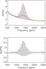 |
Fig. 1 Top panel: smoothed averaged power spectral density of four-day subseries of KIC 11244118. The red line is the severe smoothing used to normalize the spectrum (NAvPSD) shown in the lower panel (see text for details). |
To avoid subseries of low quality and to increase the S/N in the AvPSD, we first remove all subseries with a duty cycle below 50%. Then, for each subseries of each star we compute the median of the flat noise at high frequencies above 2 to 5 mHz, depending on the frequency of maximum power of the star. From the statistical analysis of these medians, we reject those subseries in which the high-frequency noise is too high. We have verified that the selection of different high-frequency ranges does not affect the number of series retained. A detailed study of the rejected series show that there is an increase in the noise level when Kepler has lost the fine pointing and the spacecraft is in “coarse” pointing mode. This is particularly important in Q12 and Q16. A new revision of the KADACS software (Mathur, Bloemen, García, in prep.) systematically removes those data points from the final corrected time series. In Table 1 we summarize the number of four-day subseries computed for each star, the number of subseries finally retained for the calculation of the AvPSD, and the total number of short-cadence Kepler quarters available.
Stars and time series used in this study.
Figure 2 shows the place of the observed stars in a seismic HR diagram. The black lines are the evolution sequences computed using the Aarhus Stellar Evolution Code (ASTEC; Christensen-Dalsgaard 2008) in a range of masses from M = 0.9 M⊙ to M = 1.6 M⊙ in steps of M = 0.1 M⊙ with a solar composition (Z⊙ = 0.0246). The target stars cover evolutionary stages from late main-sequence stars to early red giants.
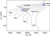 |
Fig. 2 Seismic HR diagram showing the position of the six stars analysed. The position of the Sun is indicated by the ⊙ symbol. The evolutionary tracks are computed using ASTEC (Christensen-Dalsgaard 2008). |
3. The acoustic cut-off frequency
3.1. Observations
The observed stellar power spectrum has different patterns in the eigenmode and pseudo-mode regions. In particular, the mean frequency separation, ⟨ Δν ⟩, between consecutive peaks is different below and above the cut-off frequency. In the first case, below the cut-off frequency corresponds to half the mean large frequency spacing, while above νcut it is the period of the interference pattern. In addition, a phase shift between both patterns appears in the transition region. The frequency in which the transition between the two regimes is observed corresponds to the cut-off frequency. Hence, we fit all the peaks in the spectrum (actually doublets of odd, ℓ = 1, 3, and even, ℓ = 0, 2, pairs of modes due to the small frequency resolution of 2.89 μHz) from a few orders before νmax up to the highest visible peak in the spectrum. To account for the underlying background contribution properly, which is due to convective movements at different scales, faculae, and magnetic/rotation signal, we prefer to divide the AvPSD by the same spectrum after heavy smoothing (top panel of Fig. 1) instead of using a theoretical model (e.g. Mathur et al. 2011). Although it has been demonstrated that a two-component model usually properly fits the background of stars (for more details, see Kallinger et al. 2014), the accuracy in the transition region between the eigenmode bump and the high-frequency region dominated by the HIPs is not properly described. For the purposes of this study, we are primarily interested in the transition region. Therefore, we use a simpler description of the background based on the observed spectrum itself. The length of this smoothing varies according to the evolutionary stage of the star. An example of the normalized resultant AvPSD (NAvPSD) is given in the bottom panel of Fig. 1.
A global fit to all the visible peaks in the spectrum is not possible for the following reasons: 1) it requires a huge amount of computation time owing to the high number of free parameters in the model; 2) the background is not completely flat around νmax; and 3) the large amplitude dispersion of the peaks between νmax and the HIP pattern biases the results of the smallest peaks by overestimating their amplitudes. We therefore divide the spectrum into a few orders before νmax and the photon-noise dominated region into two regions. We arbitrarily choose a frequency where the amplitudes start to be very small and separately treat the power spectrum before and after this frequency. We denote, with p-mode region, the low-frequency zone before the frequency mentioned above and the pseudo-modes region is the one after that frequency. Several tests have been performed in which the frequency separating these two regions were varied and in all cases the results remain the same.
In the p-mode region, we fit groups of several peaks at a time for which the underlying background can be considered flat. This fit depends on the evolutionary stage of the star and S/N. We checked that fitting a different number of peaks in each group does not change the final result. Appendix A shows the analysis of all the stars, and in the caption of each figure we explicitly mention the number of peaks fitted together. The pseudo-modes region can be fitted at once because 1) the background is flat (see the bottom panel of Fig. 1); 2) the range of the peak amplitudes is reduced; and 3) the number of free parameters is small. For both zones, p-mode and pseudo-mode, a Lorentzian profile is used to model the peaks using a maximum likelihood estimator. We are only interested in the frequency of the centroids of the peaks, and for that a Lorentzian profile is a good approximation. In Figs. 3 and 4 we show the results of the fits for KIC 3424541 in the p-mode and pseudo-mode regions. The figures for the other stars can be found in Appendix A.
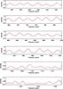 |
Fig. 3 Sections of the NAvPSD used to fit the eigenmode region in groups of six modes in KIC 3424541. The red line represents the final fit. |
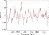 |
Fig. 4 Pseudo-mode region of the NAvPSD in KIC 3424541. The red line is the result of the fit. |
After fitting the two parts of the spectra, we compute the frequency differences of consecutive peaks: νn − νn − 1. As an example, the resultant frequency differences for KIC 3424541 are plotted in Fig. 5.
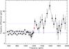 |
Fig. 5 Consecutive frequency differences of KIC 3424541. The blue dashed and dotted lines are the weighted mean value of the frequency differences in the p-mode (20.75 ± 0.20 μHz) and pseudo-mode regions (37.31 ± 1.58 μHz), respectively. The red symbol represents the estimated cut-off frequency, νcut = 1210.67 ± 15.70 μHz. |
Two different regions are clearly visible in the frequency differences of KIC 3424541. A portion of these differences, those at lower frequencies, are centred around 20.75 μHz, corresponding approximately to half of the large spacing, Δνmodes/ 2 (see Table 2) and owing to the alternation between odd and even modes. At a certain frequency, between 1200 and 1230 μHz, the frequency separations increase and remain roughly constant around 37.31 μHz, although with a higher dispersion; see the next section for further details. The observed acoustic cut-off frequency, νcut, lies in the transition region where the differences jump from the p-mode region to the pseudo-mode zone. We define this position as the mean frequency between the two closest points to this transition, represented by a red symbol in Fig. 5 for KIC 3424541. The results of this analysis for the six stars studied here are given in Table 2.
Stellar parameters I.
3.2. Comparison between the observed and theoretical cut-off frequency
As noted in Sect. 1, the cut-off frequency at the stellar surface scales approximately as  , suggesting that we may compare the observational cut-off frequency with that computed from the spectroscopic parameters. However, for our set of stars, the spectroscopic log g has large uncertainties (see Bruntt et al. 2012) and a direct test is not possible. Alternatively, it has been demonstrated empirically that the frequency of maximum mode amplitude νmax follows a similar scale relation (see Bedding & Kjeldsen 2003). As is seen in Fig. 6, the observational data show a linear relation between νmax and νcut, although some stars deviate 2σ from it. In fact, from a theoretical point of view, one does not expect this linear relation to be accurate enough at the level of the observational errors. As shown below, values of νcut can deviate by as much as 10% from the scale relation for representative models of our stars. On the other hand, following Chaplin et al. (2008), where theoretical values of νmax based on stochastic mode excitation were computed, one can find departures from the scale relation as large as 25% for a model of a star with M = 1.3 M⊙ and νmax ~ 1500 μHz.
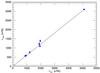 |
Fig. 6 Observed cut-off frequencies νcut versus maximum mode amplitude frequencies νmax. Blue points with errors are values for the six stars considered here and the Sun (the rightmost point). A straight line through the Sun has been drawn for guidance. |
We can gain a deeper insight by comparing the observational and theoretical results in the νcut–Δν plane. For the theoretical calculations, we use a set of models computed with the “Code d’Évolution Stellaire Adaptatif et Modulaire” (CESAM) code (Morel & Lebreton 2008). These correspond to evolutionary tracks from the zero-age main sequence up to the red-giant phase, with masses between M = 0.9 M⊙ and M = 2.0 M⊙, and helium abundances between Y = 0.25 and Y = 0.28. Models with and without overshooting were considered. Other parameters were fixed to standard values; for example, the metallicity was fixed to Z = 0.02. Finally, the CEFF equation of state (Christensen-Dalsgaard & Däppen 1992) and a T(τ) relation derived from a solar atmosphere model were used.
In theoretical computations, a standard upper boundary condition for eigenmodes is to impose in the uppermost layer the simple adiabatic evanescent solution for an isothermal atmosphere. In this case eigenmodes have frequencies below a cut-off frequency given by ωcut = 2πνcut = c/ 2H, where H is the density scale height. This is strictly speaking the cut-off frequency for radial oscillations, which is accurate for low-degree modes. To better fulfil the quasi-isothermal requirement, the boundary condition should be placed near the minimum temperature. For the Sun, this corresponds to an optical depth of about log τ = −4. Another advantage of using this sort of low optical depth is that at this position the oscillations are not too far from being adiabatic, at least compared to the photosphere. In our computations, we used this value as the uppermost point for all the models, but for some red giant stars we found that the maximum value of ωcut(r) in the atmosphere can be located at higher optical depths; hence, we took that maximum value as representative of the observed ωcut. From an interpolation to the solar mass and radius (with Y = 0.25 fixed), we obtained a value of νcut = 5125 μHz for the Sun from our set of models, which is in agreement with the observed value: νcut = 5106.41 ± 61.53μHz (Jiménez 2006). If model S (Christensen-Dalsgaard et al. 1996) is considered, the differences are a little larger, about 4%. It is important to remember that the solar νcut changes with the magnetic activity cycle (Jiménez et al. 2011); thus, some additional dispersion in the observed stellar values could be due to that effect.
For the large separation, the theoretical and observed values can be computed using the same approach. Specifically, we computed the large separation Δνmodes from a polynomial fit of the form (ν − ν0)/(n − n0) = ∑ iaiPi(x), where n is the radial order and ν0 is the radial frequency closest to νmax with radial order n0. For the models, ν0 is estimated assuming a linear relation to the cut-off frequency. The frequencies considered are those of the ℓ = 0 modes with radial orders n = n0 ± 4. Pi(x) is the Legendre polynomial of degree i, and x is the frequency normalized to the interval [−1,1 ]. We used third order polynomial. From the Tasoul equation we expect that a0 ≡ Δνmodes ≃ Δν, whereas other terms mostly contain upper-layer information. We use only radial oscillations because, for evolved stars, the mixed character of some modes can introduce complications. For the Sun, we obtain Δνmodes = 134.9 μHz from the observations and Δνmodes = 136.0 μHz from model S.
Figure 7 shows νcut against the large separation Δνmodes for our set of models and the observed stars. At first glance, there is rough agreement between the observed and theoretical calculations, but for the group of stars with νcut ~ 2000 μHz, it seems hard to explain the dispersion in their Δνmodes values.
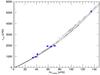 |
Fig. 7 νcut versus Δνmodes for our set of theoretical models (grey dots). Blue points correspond to the observed stars, including the Sun (upper-right point). |
We can proceed by taking the values of Teff into account. First, given the approximated scale relation for νcut, we compute the residuals 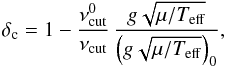 (1)where
  = 5079.5 μHz is a reference cut-off frequency, corresponding to a model in our data set close to the Sun (M = 1 M⊙, R = 1.004 R⊙, Y = 0.25,
  = 5799.2 K). The Teff values are shown in Fig. 8. As seen in the figure, the differences can be as large as | δc | ≈ 10%. In fact, the scale relation is derived theoretically by approximating the density scale height, H, by the pressure scale height, Hp, which is strictly valid in an isothermal atmosphere, and further by taking the equation of state of a mono-atomic ideal gas. In Fig. 8, the blue points correspond to the relative differences δa obtained by replacing in Eq. (1) ωcut = c/ 2H by ωa = c/ 2Hp. Thus, the first condition introduces the highest departures from the scale relation, which was expected because in the range of Teff considered, the gas is mainly mono-atomic at the surface.
Nevertheless, as seen in Fig. 8, δc is mainly a function of Teff. Hence, the scale relation can be improved if we subtract a polynomial fit from δc. We only considered models with Teff< 7000 K and νcut> 500μHz in that fit because this range includes all the stars used in the present study. For a better fit we also consider the dependence of δc on νcut. In particular, the red points in Fig. 8 are obtained by replacing νcut in Eq. (1) by ![Mathematical equation: \begin{eqnarray} \nucut^* &=& \nucut \bigg[ 1 - (0.0004 -0.0057 x - 1.0684x^2 +0.0543y \nonumber \\ && +~ 0.1265 x y -0.7134 x^2 y) \bigg] \frac{\nucut (\odot)} {\nucut^* (\odot)}, \label{eq:nucef} \end{eqnarray}](/articles/aa/full_html/2015/11/aa26469-15/aa26469-15-eq146.png) (2)where
(2)where  and
and  . The standard deviation for these residuals is 0.3%. Hence, the modified cut-off frequencies, which we calibrated on the Sun, deviate by 1σ = 0.3% from the scaling relation, at least for our set of models.
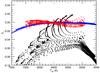 |
Fig. 8 Relative differences δc as a function of Teff (black dots). Blue points are the same relative differences but considering the isothermal cut-off frequency ωa instead of ωc. Red points are the residuals after correcting with the polynomial fit indicated in the text. The fit is limited to models with Teff< 7000 K and νcut> 500μHz. |
Stellar parameters II.
With a similar approach, we compute the deviation of Δνmodes from its expected scale relation, namely, 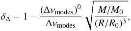 (3)where (Δνmodes)0 is the value for our reference model, the same as the value used in νcut. This quantity is shown in Fig. 9 for our set of models.
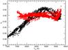 |
Fig. 9 Relative differences δΔ versus Teff for the set of models indicated in the text (black dots). The red points are the residuals after the polynomial fit. This fit is limited to models with Teff< 7000 K and Δν> 10 μHz. |
From Fig. 9 we can determine that the differences between the large separation computed from p-modes and the scaling relation can be as large as 5% for solar-like pulsators with Teff< 7000 K. However, as shown in this figure, the differences δΔ depend mainly on Teff. This was previously noted by White et al. (2011) and allows for a correction to Δνmodes to obtain a better estimate of the mean density. Here we use a fit similar to that considered for νcut. As in the previous case, we have considered only those models with Teff< 7000 K and Δνmodes> 10 μHz, which include all the stars used in the present work. The red points in Fig. 9 correspond to the residuals obtained after replacing Δνmodes in Eq. (3) by ![Mathematical equation: \begin{eqnarray} \dnumodes^* \!\!\!&&= \dnumodes \bigg[ 1 -(0.0023 -0.1123 x - 0.7309x^2 \nonumber \\ &&{-\,0.0299 z -0.0067 x z + 1.2461 x^2 z ) \bigg] } \frac{\dnumodes (\odot)} {(\dnumodes)^* (\odot)} \label{eq:dnuef}, \end{eqnarray}](/articles/aa/full_html/2015/11/aa26469-15/aa26469-15-eq193.png) (4)where and z = Δνmodes/ (Δνmodes)0−1 with (Δνmodes)0 = 135.4μHz. The standard deviation for these residuals is 0.6%. Given the differences between the observed and theoretical values for the Sun, we calibrated Eq. (4) to the observed solar value.
(4)where and z = Δνmodes/ (Δνmodes)0−1 with (Δνmodes)0 = 135.4μHz. The standard deviation for these residuals is 0.6%. Given the differences between the observed and theoretical values for the Sun, we calibrated Eq. (4) to the observed solar value.
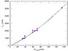 |
Fig. 10 Effective |
Figure 10 shows  against
  for our set of models (black points) and the observed stars including the Sun (blue points). Whereas the scattering in the theoretical values are substantially reduced, the observational values are not. Hence, if the error estimates are correct, we must conclude that the observational cut-off frequencies do not completely agree with the theoretical estimates. Moreover, the red points in Fig. 10 are proportional to the observed values of the frequency of maximum amplitude scaled to the Sun, (νcut/νmax)⊙νmax. For our limited set of stars, νmax follows the scaling relation better than . This is a little surprising because, as noted before, theoretically, we would expect the opposite, even more so when the effective is used.
This result can be understood in terms of the inferred surface gravity since we can use either νmax or νcut to estimate log g. The results are summarized in Table 3 and compared to the spectroscopic log gsp. To estimate the errors in log gνmax we only considered the observational errors in νmax and Teff, while for log gνcut we have included the 1σ value of 0.3% found in the scaling relation plus an error in μs derived from assuming an unknown composition with standard stellar values. In particular, we have taken ranges of Y = [ 0.24,0.28 ] and Z = [ 0.01,0.03 ] for the helium abundance and the metallicity, respectively, and thus estimated the error in the mean molecular weight μs by some 5%. As expected, the values obtained from log gνmax are quite similar to those reported by Bruntt et al. (2012) because they are based on the same global parameters with very similar values. The values derived from νmax and νcut are also much closer to each other than those derived spectroscopically, which, as mentioned before, have large observational uncertainties.
4. The HIP region
4.1. Observations
Using Sun-as-a-star observations from the GOLF instrument on board SoHO, García et al. (1998) uncovered the existence of a sinusoidal pattern of peaks above νcut, as the result of the interference between two components of a travel wave generated on the front side of the Sun with a frequency ν ≥ νcut, where the inward component returns to the visible side after a partial reflection on the far side of the Sun (see Fig. 3 in García et al. 1998). Therefore, the frequency spacing of ~70 μHz found in the Sun corresponded to the time delay between the direct emitted wave and that coming from the back of the Sun, corresponding to waves behaving like low-degree modes, i.e. a delay of four times the acoustic radius of the Sun (~3600 s). This value is roughly half of the large frequency spacing of the star, which we call Δν1. García et al. (1998) also speculated that, above a given frequency, a second pattern should become visible with a double frequency spacing (close to the large frequency separation), Δν2 ~ 140 μHz. This pattern (for a theoretical description, see Kumar 1993), which is usually visible in imaged instruments (Duvall et al. 1991), corresponds to the interference between outward emitted waves and the inward components, which arrive at the visible side of the Sun after the refraction at the inner turning point (non-radial waves).
Two sine waves are fitted above the cut-off frequency to obtain a global estimate of the frequency of the interference patterns in the HIP region of our sample of stars. The amplitudes and frequencies of both sine waves are summarized in Table 2. We also reanalysed the GOLF and VIRGO data, following the same procedure using at a higher frequency range of between 7 and 8 mHz, compared to the original analyses performed by García et al. (1998) and Jiménez (2006). With this approach, we have been able to obtain the second periodicity at ~140 μHz (see Table 2).
We tried fitting various functions and opted for the simplest one. Indeed, the amplitude of the interference patterns decreases with frequency in a manner that is close to an exponential decrease. The additional parameters required give more unstable fits with a heavy dependence on the guess parameters. We preferred this approach because we obtained the same qualitative results leading to the same classification of stars. In future studies, we will look for a better function for the fit, i.e. one more suited to the observations, in a larger set of stars. We are already working in this direction but this investigation is beyond of the scope of this paper.
According to the fitted amplitudes, we can classify the stars into two groups: those in which the two amplitudes of the sine waves, A1 and A2, are similar (KIC 7940546, KIC 9812850, KIC 11244118), and those in which A2 is much larger than A1 (KIC 3424541, KIC 7799349, KIC 11717120). An example of each group of stars is given in Fig. 11 for stars KIC 7940546 and KIC 11717120. The error bars of the fitted amplitudes are large because the actual amplitudes of the interference patterns decrease in a quasi-exponential way that has not been taken into account here. We favoured the fits with constant amplitudes to avoid adding more unknown parameters to the fit.
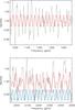 |
Fig. 11 HIPs region of KIC 11717120 (top), where the HIP pattern is dominated by the sine wave (red line), owing to the interference between direct and refracted waves; and the region of KIC 7940546 (bottom), where the two HIP patterns can be determined. The blue and green lines in the bottom panel correspond to the two fitted sine waves with frequencies Δν1 and Δν2, respectively. We shifted the green and blue lines by 0.05 for clarity. The red line is the actual fit. |
The stars of the first group have larger Δνmodes than the other three stars, which implies a correlation with the evolutionary state of the stars. Starting with the Sun on the main sequence, the HIP pattern is dominated by interference waves partially reflected at the back of the Sun (for the solar case A1 is much bigger than A2). When the stars evolve, the HIP pattern due to the interference of direct with refracted waves in the stellar interior is more and more visible and becomes dominant for evolved RGB stars with Δνmodes below ~40 μHz.
4.2. HIPs and stellar evolution
To reproduce the periodic signals expected from the pseudo-mode spectrum theoretically, we follow the interpretation given by Kumar (1993) and García et al. (1998) and assume that waves are excited isotropically at a point very close to the photosphere. The observed spectrum of the pseudo-modes is then interpreted as an interference pattern between outgoing and ingoing components, possibly including successive surface reflections. In what follows, we summarize the basic concepts and apply them to stars at different evolutionary stages.
We start with a gravito–acoustic ray theory approximation with the following dispersion relation (see e.g. Gough 1986, 1993): 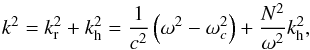 (5)where kr is the radial component of the wave number,
  , L = l(l + 1) the horizontal component, N is the buoyancy frequency, ωc is a generalized cut-off frequency given by
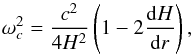 (6)and H is the density scale height. In the ray approximation, the turning points are given by kr = 0, whereas the ray path is determined by the group velocity. For the spherically symmetric case, the rays are contained in a plane with a path given by dθ/dr = vθ/ (rvr) . Here, r and θ are the usual polar coordinates and the group velocity vg = (vr,vθ) = (∂ω/∂kr,∂ω/∂kh) has the following components:
 ![Mathematical equation: \begin{equation} \vec{v}_{\rm g} = \left( \,\frac{k_r \omega^3 c^2} {\omega^4 - k_{\rm h}^2 c^2 N^2} , k_{\rm h} \, \omega \, c^2 \left[ \frac{\omega^2 - N^2}{\omega^4 -k_{\rm h}^2 c^2 N^2} \right] \,\right) \cdot \end{equation}](/articles/aa/full_html/2015/11/aa26469-15/aa26469-15-eq219.png) (7)According to the ray theory, the general solution of the wave equation can be expressed as a superposition of rays of the form ψω(r,t) = Aω(r)exp [ i(ωt ± ∫sk ds) ], where the two signs corresponds to outgoing and ingoing waves and the integral is computed over the ray path s, including additional reflections where appropriate. For every reflection, a constant phase shift must be introduced. In particular, for a ray travelling from an inner turning point r1 to an outer turning point r2, this integral can be expressed as
(7)According to the ray theory, the general solution of the wave equation can be expressed as a superposition of rays of the form ψω(r,t) = Aω(r)exp [ i(ωt ± ∫sk ds) ], where the two signs corresponds to outgoing and ingoing waves and the integral is computed over the ray path s, including additional reflections where appropriate. For every reflection, a constant phase shift must be introduced. In particular, for a ray travelling from an inner turning point r1 to an outer turning point r2, this integral can be expressed as 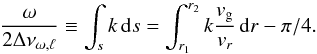 (8)For low-degree acoustic waves
  , that is, Δνω,ℓ ≈ Δν.
Considering a wave excited very close to the surface with an outgoing component of amplitude Aωℓ and an ingoing component that emerges at the surface with an amplitude  after its first internal traversal, and with an amplitude of
  after a subsequent partial surface reflection on the back side of the star, the contribution to the amplitude spectrum can be expressed as
 ![Mathematical equation: \begin{equation} \sum_{\omega,\ell} \left( V_{\omega,\ell} A_{\omega, \ell} + A'_{\omega, \ell} {\rm e}^{{\rm i}\delta} \bigg[V'_{\omega,\ell} {\rm e}^{-{\rm i} \omega/\Delta\nu_{\omega,\ell} }+ V''_{\omega,\ell} R(\omega) {\rm e}^{-2{\rm i}\omega/\Delta\nu_{\omega,\ell}} \bigg] \right) , \label{eq:interf1} \end{equation}](/articles/aa/full_html/2015/11/aa26469-15/aa26469-15-eq230.png) (9)where Vω,ℓ,
(9)where Vω,ℓ,  and
and  are visibility factors and δ is a phase constant that depends on the type of radiation emitted. The reflection coefficient R is expected to be a monotonically decreasing function of frequency (for further details see Kumar 1993). We also assume that, for stochastically excited waves, the amplitudes and the visibility factors are a smooth function of frequency. Hence, the amplitude spectrum is modulated with the periodic functions cos(ω/ Δνω,ℓ) and cos(2ω/ Δνω,ℓ). Although in principle different values of Δνω,ℓ can be expected in different frequency ranges and for different degrees ℓ, their differences are too weak, and in the present study we fitted the data to just two periodic components, Δν2 = Δνω,ℓ and Δν1 = Δνω,ℓ/ 2. In addition, in some stars one of the signals could be masked by low-visibility factors or low reflection coefficients.
To illustrate the problem, we considered a 1.1 M⊙ evolution sequence and plotted rays for two typical frequencies in the pseudo-mode range and three evolutionary stages in Fig. 12. Top panels are for frequencies ω = 1.1ωa while bottom panels are for ω = 1.5ωa. On the other hand, the star evolves from left (zero age main sequence, ZAMS) to right (red giant branch, RGB). For clarity, surface reflections have been omitted.
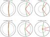 |
Fig. 12 Ray path for waves with angular degrees ℓ = 1 (red) and ℓ = 2 (green) for a 1.1 M⊙ model evolution sequence. For clarity, surface reflections have been omitted. The upper part shows rays with a frequency a 10% greater than the acoustic cut-off frequency ωa, while the bottom panels corresponds to rays with a frequency 50% greater than ωa. The large separation indicated is the integral |

For the model close to the ZAMS (leftmost panels), the inward rays emerge at the surface making angles between 160° and 180° with the outward component. In this case, the outward and inward components of a given wave can only be simultaneously visible if they lie too close to the limb. Hence, their signal corresponding to Δν2 ≃ Δν is highly attenuated in the power spectrum. In contrast, after one surface reflection the angle between the outward and inward components lies in the range 0° to 35°. This interference would give the Δν1 ≃ Δν/ 2 separation and, hence, if it had the same intrinsic amplitude as the former, the Δν1 separation would be easier to observe. In this case, however, the inward rays are only partially reflected on the far side (e.g. Kumar 1993) and hence the attenuation factor, corresponding to R(ω) in Eq. (9), is high. Since the actual observations show that in the Sun the dominant separation in the HIP pattern is Δν1 (García et al. 1998), we can use this case as a qualitative reference between the two competing factors. For model S, we obtain Δν1 = 72 μHz with our fit, for which a frequency range ~[5200, 6600] μHz was used. This result is in agreement with the observational value of 70.46 ± 2 μHz found by García et al. (1998). As mentioned in section 4.1, we reanalysed the solar data (GOLF and VIRGO Sun photometers) and obtained Δν1 ~ 70 μHz (see Table 2), in agreement with previous values given in the literature. At higher frequencies we refitted the data with two sinusoidal components and found Δν2 ~ 140 μHz (Table 2). This value is in agreement with the theoretical prediction already described by Garcia et al. (1998) if we assume that the photosphere is the only source of partial wave reflection. However, in this case the amplitude is much smaller because only waves close to the limb contribute to this interference pattern.
As the stars evolve, the angle between the outward ray and the first surface appearance of the inward refracted ray becomes smaller for the ℓ = 1 pseudo-modes. This is clearly apparent in Fig. 12. Hence, the Δν2 ≃ Δν interference pattern becomes easier to observe (higher observed A2 amplitudes). This phenomenon is due to the transition between acoustic rays smoothly bending through the stellar interior, and waves where the density scale height in the stellar inner structure becomes close to their wavelength and the ray behaviour at the inner turning point is closer to a two-layer reflection. Finally, in the most evolved model in Fig. 12 (upper and bottom right panels) the ℓ = 1 waves have a gravity character close to the centre that bends the ray into a loop.
We used Eq. (9) to reproduce the observed power spectrum schematically, and considered ray traces for a continuum spectrum of waves with frequencies between the acoustic cut-off frequency at the surface and about 1.5 times that value. This frequency interval spans approximately the observed pseudo-mode frequency range. Since we are only interested in reproducing the periodicities of the pseudo-mode spectra, constant amplitudes were considered as well as visibility factors either constant or proportional to cosΘ/2, where Θ, is the angular distance between the outward and inward waves. We determine the periodic signal in the spectrum with a non-linear fit to the above equation.
Figure 13 shows the angular distance between the inward and outward components before any surface reflection against the large separation Δν for models in a 1.1 M⊙, Y = 0.28 evolution sequence with the code and physics indicated in Sect. 3.2. Here, mean values of the angular distance are computed by averaging those of the ray traces in the frequency range indicated above. Pseudo-modes with ℓ = 1 and 2 are averaged separately. Since no surface reflection is considered, these waves form the Δν2 pattern.
Looking at the behaviour of the ℓ = 1 pseudo-modes in Fig. 13 (red points), we may conclude that for M = 1.1 M⊙ stars that evolve to a Δν below some given threshold between 90 μHz and 60 μHz (corresponding to evolved main-sequence stars as that shown in the middle panel of Fig. 12), the Δν2 pattern should become visible. Indeed, a smaller angular distance means more disc-centred interferences favouring a higher A2. The critical Δν slightly changes with mass, which is lower for higher masses. In any case, all the stars in Table 2, except the Sun, are evolved to a point where the pattern with Δν2 could be easily observed, as is in fact the case.
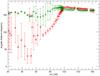 |
Fig. 13 Angular distance between inward and outward waves against Δν for a 1.1 M⊙ evolution sequence. Frequencies between the acoustic cut-off frequency at the surface and about 50% greater than ωa are considered. For every model in the sequence, frequency-averaged values of the angular distance and 1σ dispersions are calculated separately for ℓ = 1 (red points) and ℓ = 2 (green points) waves. An angle of 180° means no inner reflection. |
Regarding the ℓ = 2 pseudo-modes, it can be seen in Fig. 13 that the angle distance always remains above some 150° and hence this degree only contributes to the Δν1 period in the pseudo-mode spectrum. The higher dispersion in the angular distance for models with a large separation between Δν = 60 and 90 μHz (evolved main-sequence stars and subgiants), clearly visible in Fig. 13, deserves a comment. According to the dispersion relation we used, for models evolved near the Terminal Age Main Sequence (TAMS) the characteristic frequencies of the ℓ = 2 waves become complex in a small radius interval above the core, thus increasing the resonant cavity of the pseudo-modes within a limited frequency range. An example of the ray path of these kinds of waves is shown in the middle of the bottom panel of Fig. 12 (green line). Here, the ray trace close to the centre is not of the acoustic type and the emerging ray is consequently scattered. Althought these results may be questionable in terms of the validity of the approximation used here, they do not have any observable consequences.
For the three most evolved stars in our data set the interference pattern coming from waves reflected back at the surface with period Δν1 is not observed. The fact that for evolved stars the signal from the ℓ = 1 pseudo-modes do not suffer any attenuation from surface reflections may explain why for stars evolved to the RGB the Δν1 signal becomes completely masked. However, it is interesting to note the another, possibly superimposed, cause for this circumstance. In principle, one might expect that radial waves propagates all the way from the surface to the centre and hence contributes to the signal only once reflected back, hence, with a period Δν1. However there is a point in the evolution where the cut-off frequency in the core rises above the typical pseudo-mode frequencies, in which case the ray theory introduces an inner reflection. Although a plano-parallel approximation is questionable in terms of the wavelength-radius relation when we are too close to the centre, this approximation allows us to estimate the transmission coefficient T, as in the one-dimensional problem1. If the equation T = 1/(1 + e2K) is used with 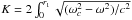 , r1 being the point where kr = 0, it happens that, for red giant stars, radial waves in the observed frequency range of the pseudo-mode spectrum are mostly reflected at the core edge. Thus, at this stage, radial pseudo-modes also contribute to the Δν2 signal and, hence, the Δν1 period would hardly be observed.
We now discuss the relation between the large separation obtained from the eigenmodes, Δνmodes, and those corresponding to the pseudo-modes, Δν1 and Δν2. First, we verified that for waves with ℓ = 0 the phase travel time is always close to the asymptotic acoustic value,  . Hence, when these acoustic waves contribute to the HIPs after a surface reflection they give Δν1 ≃ Δνmodes/ 2. In addition, most of the ℓ = 2 and, in some stars, ℓ = 1 travelling waves have similar acoustic characteristics, which also contributed to the same interference period. This is in agreement with Table 2, where both frequency separations match within the errors.
The case of Δν2 is different. The grey points in Fig. 14 are the periods of the interference pattern computed according to Eq. (9) for travelling waves and no surface reflection. A wide range of masses and evolutionary stages from main sequence to the base of the red-giant branch were included. The red points are the observed Δν2 values while blue points are 2Δν1 when observed, including the Sun. The black line corresponds to Δνmodes = Δν2. From Fig. 14 we can see that, for Δνmodes = 60–80 μHz, there are models with Δν2< Δνmodes. In fact, they correspond to evolved stars up to the end of the main sequence or the subgiant phase, as it is the case for our sample of stars. Although the order of magnitude of the phase delay found for our models is similar to the observed one for this type of star, it is also apparent from the figure that KIC 1124411 (Δνmodes ~ 70 μHz) has a large separation, which is too high for this delay to appear. We obtain a mass of ~1 M⊙ either by applying the scaling relations to νmax and Δνmodes via an isochrone fit. The upper right corner of Fig. 12 is representative of this star. Hence we expect to observe the signal Δν2 from waves reflected in the interior but our computations do not show any significant delay in the phase of the ℓ = 1 compared to the radial oscillations. Further work is need here; in particular, the asymptotic theory that we have used could be inadequate for these kinds of details.
For stars with the lower Δνmodes, two of them have Δν2 ≃ Δνmodes and one star (KIC 11717120) has Δν2< Δνmodes. With our isochrones fitting, we find that the latter is at the base of the RGB as well as KIC 7799349, thus we have two different results for stars with very similar parameters. With our simple simulation for models at this evolutionary stage we have both signals since, as noted above, radial oscillations are partially reflected at the core edge and, for these stars, Δν2 ≃ Δνmodes. The observed period is a weighted average, but for a better comparison with the observations proper amplitudes need to be computed.
 |
Fig. 14 Grey points are periods of the pseudo-mode interference pattern for evolution sequences with masses between 0.9 M⊙ and 2 M⊙. For the sake of clarity, only waves with no surface reflections are shown. Red points correspond to the observed Δν2 values and blue points correspond to 2Δν1 when observed. The black line corresponds to Δνmodes = Δν2. |
5. Conclusions
We measured the acoustic cut-off frequency and characteristics of the HIPs in six stars with solar-like pulsations observed by the Kepler mission. A comparison with the observed νmax shows a linear trend with all stars lying in ~2σ. As a result, the values of log g derived from νcut agree to within the same accuracy with those derived from νmax, but are substantially different in some cases from the values derived from spectroscopic fits (see Table 3). When comparing the stars with the models in the νcut–Δν plane, we found a departure in νcut from the expected values. It is possible to calculate, with theoretical information, a measurable function  that scales as
  with no more than 0.3% deviation (for our set of models representative of our star sample and the Sun), however, we find that the observational does not follow this relation so accurately. Rather surprisingly, we found that the frequency of maximum power, νmax, follows the linear relation within errors. Hence, for the evolved stars considered in the present study it must be concluded that νmax gives an even better estimate of log g than νcut with the current uncertainties.
Given the observed characteristics of the HIPs, our set of six stars can be divided into two groups. In three stars: KIC 3424541, KIC 7799349, and KIC 11717120, the only visible pattern is that due to the interference with inner refracted waves in the visible disc of the star and not close to the limb. In the other three stars (KIC 7940546, KIC 9812850, and KIC 11244118), the pattern is because partial reflection of the inward waves at the back of the star is also detected. This different behaviour is related to the wide spacing of the star, which reveals a dependence on the evolutionary stage.
When present, the period Δν1, which corresponds to the interference of outward waves with their inward counterpart once reflected on the far side, always agrees with half the large separation, although, like the Sun, their values are a little higher. This result is also found theoretically, and the large separation derived from the pseudo-modes is closer to ∫dr/c. However, the period Δν2 corresponding to waves refracted in the inner part of the star can be substantially different from the large frequency separation. We interpret this by claiming the presence of waves of a mixed nature. For these stars, the phase ∫kdl is smaller compared to the radial acoustic case. Although a detailed analysis is beyond the scope of the present study, simple ray theory calculations reveal that this kind of a phenomenon is expected with the same order of magnitude.
The pseudo-mode spectrum reveals information from the surface properties of the stars through νcut and from the interior, at least in the cases where the period Δν2 is lower than the large separation derived from the eigenmodes. We are aware that the interference periods derived observationally are power-weighted averages and for a proper comparison with theoretical expectation some work along these lines should be addressed. This might be accomplished by computing transmission coefficients so that more realistic theoretical simulations of the interference phenomenon can be performed.
Online material
Appendix A: Figures of the other stars
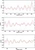 |
Fig. A.1 Fitted (red line) NAvPSD of KIC 7799349 by groups of nine peaks in the low-frequency range (p-modes). |
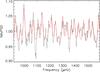 |
Fig. A.2 Fitted (red line) NAvPSD of KIC 7799349 in the high-frequency range (pseudo-modes). |
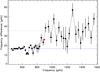 |
Fig. A.3 Consecutive frequency differences (KIC 7799349); that is, the separations between the fitted peaks for NAvPSD. Two levels are shown: one around Δν/ 2, corresponding to p-modes (blue dashed line with a weighted mean of 16.64 ± 0.09 μHz), and other around Δν, corresponding to pseudo-modes (blue dotted line with a weighted mean of 35.23 ± 1.52 μHz). The red symbol is the estimate of the acoustic cut-off frequency (895.47 ± 15.38 μHz). |
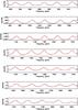 |
Fig. A.4 Fitted (red line) NavPSD of KIC 7940546 by groups of five peaks in the low-frequency range (p-modes). |
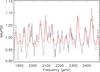 |
Fig. A.5 Fitted (red line) NAvPSD of KIC 7940546 in the high-frequency range (pseudo-modes). |
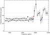 |
Fig. A.6 Consecutive frequency differences (KIC 7940546), that is, the separations between the fitted peaks for NAvPSD. Two levels are shown: one around Δν/ 2, corresponding to p-modes (blue dashed line with a weighted mean of 29.50 ± 0.07 μHz), and other around Δν, corresponding to pseudo-modes (blue dotted line with a weighted mean of 45.71 ± 2.12 μHz). The red symbol is the estimate of the acoustic cut-off frequency (1940.59 ± 20.71 μHz). |
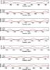 |
Fig. A.7 Fitted (red line) NAvPSD of KIC 9812850 by groups of four peaks in the low-frequency range (p-modes). |
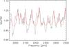 |
Fig. A.8 Fitted (red line) NAvPSD of KIC 9812850 in the high-frequency range (pseudo-modes). |
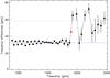 |
Fig. A.9 Consecutive frequency differences (KIC 9812850); that is, the separations between the fitted peaks for NAvPSD. Two levels are shown: one around Δν/ 2, corresponding to p-modes (blue dashed line with a weighted mean of 32.53 ± 0.12 μHz), and other around Δν, corresponding to pseudo-modes (blue dotted line with a weighted mean of 58.13 ± 2.39 μHz). The red symbol is the estimate of the acoustic cut-off frequency (1898.08 ± 24.29 μHz). |
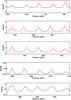 |
Fig. A.10 Fitted (red line) NAvPSD of KIC 11244118 by groups of five peaks in the low-frequency range (p-modes). |
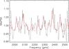 |
Fig. A.11 Fitted (red line) NAvPSD of KIC 11244118 in the high-frequency range (pseudo-modes). |
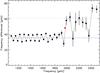 |
Fig. A.12 Consecutive frequency differences (KIC 11244118); that is, the separations between the fitted peaks for NAvPSD. Two levels are shown: one around Δν/ 2, corresponding to p-modes (blue dashed line with a weighted mean of 35.54 ± 0.08 μHz), and other around Δν, corresponding to pseudo-modes (blue dotted line with a weighted mean of 61.02 ± 2.19 μHz). The red symbol is the estimation of the acoustic cut-off frequency (1968.69 ± 21.48 μHz). |
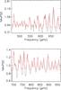 |
Fig. A.13 Fitted (red line) NAvPSD of KIC 11717120 by groups of sixteen peaks in the low-frequency range (p-modes). |
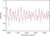 |
Fig. A.14 Fitted (red line) NAvPSD of KIC 11717120 in the high-frequency range (pseudo-modes). |
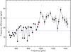 |
Fig. A.15 Consecutive frequency differences (KIC 11717120); that is, the separations between the fitted peaks for NAvPSD. Two levels are shown: one around Δν/ 2, corresponding to p-modes (blue dashed line with a weighted mean of 16.71 ± 0.09 μHz), and other around Δν, corresponding to pseudo-modes (blue dotted line with a weighted mean of 29.85 ± 0.66 μHz). The red symbol is the estimation of the acoustic cut-off frequency (958.38 ± 11.56 μHz). |
For radial oscillations, the full adiabatic equations are of second order and, hence, a WKB analysis can be obtained without the approximations assumed in the dispersion relation Eq. (5). The qualitative results given in this paragraph rely solely on the assumption of a one-dimensional problem.
Acknowledgments
The authors of this paper thank Dr. J. Ballot, Dr. G. R. Davies, and P. L. Pallé for useful comments and discussions, as well as the entire Kepler team, without whom these results would not be possible. Funding for this Discovery mission is provided by NASA Science Mission Directorate. This research was supported in part by the Spanish National Research Plan under project AYA2010-17803. This research was supported in part by the National Science Foundation under Grant No. NSF PHY05-51164. R.A.G. has received funding from the European Community Seventh Framework Program (FP7/2007-2013) under grant agreement No. 269194 (IRSES/ASK), from the ANR (Agence Nationale de la Recherche, France) program IDEE (No. ANR-12-BS05-0008) “Interaction Des Étoiles et des Exoplanètes”, and from the CNES. S.M. acknowledges the support of the NASA grant NNX12AE17G.
References
- Bedding, T. R., & Kjeldsen, H. 2003, PASA, 20, 203 [Google Scholar]
- Borucki, W. J., Koch, D., Basri, G., et al. 2010, Science, 327, 977 [NASA ADS] [CrossRef] [PubMed] [Google Scholar]
- Brown, T. M., Latham, D. W., Everett, M. E., & Esquerdo, G. A. 2011, AJ, 142, 112 [NASA ADS] [CrossRef] [Google Scholar]
- Bruntt, H., Basu, S., Smalley, B., et al. 2012, MNRAS, 423, 122 [NASA ADS] [CrossRef] [Google Scholar]
- Chaplin, W. J., Houdek, G., Appourchaux, T., et al. 2008, A&A, 485, 813 [NASA ADS] [CrossRef] [EDP Sciences] [Google Scholar]
- Christensen-Dalsgaard, J. 2008, Ap&SS, 316, 13 [NASA ADS] [CrossRef] [Google Scholar]
- Christensen-Dalsgaard, J., & Däppen, W. 1992, A&ARv, 4, 267 [NASA ADS] [CrossRef] [Google Scholar]
- Christensen-Dalsgaard, J., Dappen, W., Ajukov, S. V., et al. 1996, Science, 272, 1286 [CrossRef] [Google Scholar]
- Domingo, V., Fleck, B., & Poland, A. I. 1995, Sol. Phys., 162, 1 [NASA ADS] [CrossRef] [Google Scholar]
- Duvall, Jr., T. L., Harvey, J. W., Jefferies, S. M., & Pomerantz, M. A. 1991, ApJ, 373, 308 [Google Scholar]
- Fröhlich, C., Romero, J., Roth, H., et al. 1995, Sol. Phys., 162, 101 [NASA ADS] [CrossRef] [Google Scholar]
- Gabriel, A. H., Grec, G., Charra, J., et al. 1995, Sol. Phys., 162, 61 [NASA ADS] [CrossRef] [Google Scholar]
- García, R. A., Pallé, P. L., Turck-Chièze, S., et al. 1998, ApJ, 504, L51 [NASA ADS] [CrossRef] [Google Scholar]
- García, R. A., Hekker, S., Stello, D., et al. 2011, MNRAS, 414, L6 [NASA ADS] [CrossRef] [Google Scholar]
- García, R. A., Mathur, S., Pires, S., et al. 2014, A&A, 568, A10 [NASA ADS] [CrossRef] [EDP Sciences] [Google Scholar]
- Gilliland, R. L., Jenkins, J. M., Borucki, W. J., et al. 2010, ApJ, 713, L160 [NASA ADS] [CrossRef] [Google Scholar]
- Gough, D. O. 1986, in Hydrodynamic and Magnetodynamic Problems in the Sun and Stars, ed. Y. Osaki, 117 [Google Scholar]
- Gough, D. O. 1993, in Astrophysical Fluid Dynamics – Les Houches 1987, eds. J.-P. Zahn, & J. Zinn-Justin, 399 [Google Scholar]
- Jefferies, S. M., Pomerantz, M. A., Duvall, Jr., T. L., Harvey, J. W., & Jaksha, D. B. 1988, in Seismology of the Sun and Sun-Like Stars, ed. E. J. Rolfe, ESA SP, 286, 279 [Google Scholar]
- Jiménez, A. 2006, ApJ, 646, 1398 [NASA ADS] [CrossRef] [Google Scholar]
- Jiménez, A., Jiménez-Reyes, S. J., & García, R. A. 2005, ApJ, 623, 1215 [NASA ADS] [CrossRef] [Google Scholar]
- Jiménez, A., García, R. A., & Pallé, P. L. 2011, ApJ, 743, 99 [NASA ADS] [CrossRef] [Google Scholar]
- Kallinger, T., De Ridder, J., Hekker, S., et al. 2014, A&A, 570, A41 [NASA ADS] [CrossRef] [EDP Sciences] [Google Scholar]
- Kumar, P. 1993, in GONG 1992. Seismic Investigation of the Sun and Stars, ed. T. M. Brown, ASP Conf. Ser., 42, 15 [Google Scholar]
- Kumar, P., Duvall, Jr., T. L., Harvey, J. W., et al. 1990, in Progress of Seismology of the Sun and Stars, eds. Y. Osaki, & H. Shibahashi (Berlin: Springer Verlag), Lect. Notes Phys., 367, 87 [Google Scholar]
- Libbrecht, K. G. 1988, ApJ, 334, 510 [NASA ADS] [CrossRef] [Google Scholar]
- Mathur, S., García, R. A., Régulo, C., et al. 2010, A&A, 511, A46 [NASA ADS] [CrossRef] [EDP Sciences] [Google Scholar]
- Mathur, S., Hekker, S., Trampedach, R., et al. 2011, ApJ, 741, 119 [NASA ADS] [CrossRef] [Google Scholar]
- Morel, P., & Lebreton, Y. 2008, Ap&SS, 316, 61 [NASA ADS] [CrossRef] [MathSciNet] [Google Scholar]
- Pires, S., Mathur, S., García, R. A., et al. 2015, A&A, 574, A18 [NASA ADS] [CrossRef] [EDP Sciences] [Google Scholar]
- White, T. R., Bedding, T. R., Stello, D., et al. 2011, ApJ, 743, 161 [NASA ADS] [CrossRef] [Google Scholar]
All Tables
All Figures
|
Fig. 1 Top panel: smoothed averaged power spectral density of four-day subseries of KIC 11244118. The red line is the severe smoothing used to normalize the spectrum (NAvPSD) shown in the lower panel (see text for details). |
| In the text | |
|
Fig. 2 Seismic HR diagram showing the position of the six stars analysed. The position of the Sun is indicated by the ⊙ symbol. The evolutionary tracks are computed using ASTEC (Christensen-Dalsgaard 2008). |
| In the text | |
|
Fig. 3 Sections of the NAvPSD used to fit the eigenmode region in groups of six modes in KIC 3424541. The red line represents the final fit. |
| In the text | |
|
Fig. 4 Pseudo-mode region of the NAvPSD in KIC 3424541. The red line is the result of the fit. |
| In the text | |
|
Fig. 5 Consecutive frequency differences of KIC 3424541. The blue dashed and dotted lines are the weighted mean value of the frequency differences in the p-mode (20.75 ± 0.20 μHz) and pseudo-mode regions (37.31 ± 1.58 μHz), respectively. The red symbol represents the estimated cut-off frequency, νcut = 1210.67 ± 15.70 μHz. |
| In the text | |
|
Fig. 6 Observed cut-off frequencies νcut versus maximum mode amplitude frequencies νmax. Blue points with errors are values for the six stars considered here and the Sun (the rightmost point). A straight line through the Sun has been drawn for guidance. |
| In the text | |
|
Fig. 7 νcut versus Δνmodes for our set of theoretical models (grey dots). Blue points correspond to the observed stars, including the Sun (upper-right point). |
| In the text | |
|
Fig. 8 Relative differences δc as a function of Teff (black dots). Blue points are the same relative differences but considering the isothermal cut-off frequency ωa instead of ωc. Red points are the residuals after correcting with the polynomial fit indicated in the text. The fit is limited to models with Teff< 7000 K and νcut> 500μHz. |
| In the text | |
|
Fig. 9 Relative differences δΔ versus Teff for the set of models indicated in the text (black dots). The red points are the residuals after the polynomial fit. This fit is limited to models with Teff< 7000 K and Δν> 10 μHz. |
| In the text | |
|
Fig. 10 Effective |
| In the text | |
|
Fig. 11 HIPs region of KIC 11717120 (top), where the HIP pattern is dominated by the sine wave (red line), owing to the interference between direct and refracted waves; and the region of KIC 7940546 (bottom), where the two HIP patterns can be determined. The blue and green lines in the bottom panel correspond to the two fitted sine waves with frequencies Δν1 and Δν2, respectively. We shifted the green and blue lines by 0.05 for clarity. The red line is the actual fit. |
| In the text | |
|
Fig. 12 Ray path for waves with angular degrees ℓ = 1 (red) and ℓ = 2 (green) for a 1.1 M⊙ model evolution sequence. For clarity, surface reflections have been omitted. The upper part shows rays with a frequency a 10% greater than the acoustic cut-off frequency ωa, while the bottom panels corresponds to rays with a frequency 50% greater than ωa. The large separation indicated is the integral |
| In the text | |
|
Fig. 13 Angular distance between inward and outward waves against Δν for a 1.1 M⊙ evolution sequence. Frequencies between the acoustic cut-off frequency at the surface and about 50% greater than ωa are considered. For every model in the sequence, frequency-averaged values of the angular distance and 1σ dispersions are calculated separately for ℓ = 1 (red points) and ℓ = 2 (green points) waves. An angle of 180° means no inner reflection. |
| In the text | |
|
Fig. 14 Grey points are periods of the pseudo-mode interference pattern for evolution sequences with masses between 0.9 M⊙ and 2 M⊙. For the sake of clarity, only waves with no surface reflections are shown. Red points correspond to the observed Δν2 values and blue points correspond to 2Δν1 when observed. The black line corresponds to Δνmodes = Δν2. |
| In the text | |
|
Fig. A.1 Fitted (red line) NAvPSD of KIC 7799349 by groups of nine peaks in the low-frequency range (p-modes). |
| In the text | |
|
Fig. A.2 Fitted (red line) NAvPSD of KIC 7799349 in the high-frequency range (pseudo-modes). |
| In the text | |
|
Fig. A.3 Consecutive frequency differences (KIC 7799349); that is, the separations between the fitted peaks for NAvPSD. Two levels are shown: one around Δν/ 2, corresponding to p-modes (blue dashed line with a weighted mean of 16.64 ± 0.09 μHz), and other around Δν, corresponding to pseudo-modes (blue dotted line with a weighted mean of 35.23 ± 1.52 μHz). The red symbol is the estimate of the acoustic cut-off frequency (895.47 ± 15.38 μHz). |
| In the text | |
|
Fig. A.4 Fitted (red line) NavPSD of KIC 7940546 by groups of five peaks in the low-frequency range (p-modes). |
| In the text | |
|
Fig. A.5 Fitted (red line) NAvPSD of KIC 7940546 in the high-frequency range (pseudo-modes). |
| In the text | |
|
Fig. A.6 Consecutive frequency differences (KIC 7940546), that is, the separations between the fitted peaks for NAvPSD. Two levels are shown: one around Δν/ 2, corresponding to p-modes (blue dashed line with a weighted mean of 29.50 ± 0.07 μHz), and other around Δν, corresponding to pseudo-modes (blue dotted line with a weighted mean of 45.71 ± 2.12 μHz). The red symbol is the estimate of the acoustic cut-off frequency (1940.59 ± 20.71 μHz). |
| In the text | |
|
Fig. A.7 Fitted (red line) NAvPSD of KIC 9812850 by groups of four peaks in the low-frequency range (p-modes). |
| In the text | |
|
Fig. A.8 Fitted (red line) NAvPSD of KIC 9812850 in the high-frequency range (pseudo-modes). |
| In the text | |
|
Fig. A.9 Consecutive frequency differences (KIC 9812850); that is, the separations between the fitted peaks for NAvPSD. Two levels are shown: one around Δν/ 2, corresponding to p-modes (blue dashed line with a weighted mean of 32.53 ± 0.12 μHz), and other around Δν, corresponding to pseudo-modes (blue dotted line with a weighted mean of 58.13 ± 2.39 μHz). The red symbol is the estimate of the acoustic cut-off frequency (1898.08 ± 24.29 μHz). |
| In the text | |
|
Fig. A.10 Fitted (red line) NAvPSD of KIC 11244118 by groups of five peaks in the low-frequency range (p-modes). |
| In the text | |
|
Fig. A.11 Fitted (red line) NAvPSD of KIC 11244118 in the high-frequency range (pseudo-modes). |
| In the text | |
|
Fig. A.12 Consecutive frequency differences (KIC 11244118); that is, the separations between the fitted peaks for NAvPSD. Two levels are shown: one around Δν/ 2, corresponding to p-modes (blue dashed line with a weighted mean of 35.54 ± 0.08 μHz), and other around Δν, corresponding to pseudo-modes (blue dotted line with a weighted mean of 61.02 ± 2.19 μHz). The red symbol is the estimation of the acoustic cut-off frequency (1968.69 ± 21.48 μHz). |
| In the text | |
|
Fig. A.13 Fitted (red line) NAvPSD of KIC 11717120 by groups of sixteen peaks in the low-frequency range (p-modes). |
| In the text | |
|
Fig. A.14 Fitted (red line) NAvPSD of KIC 11717120 in the high-frequency range (pseudo-modes). |
| In the text | |
|
Fig. A.15 Consecutive frequency differences (KIC 11717120); that is, the separations between the fitted peaks for NAvPSD. Two levels are shown: one around Δν/ 2, corresponding to p-modes (blue dashed line with a weighted mean of 16.71 ± 0.09 μHz), and other around Δν, corresponding to pseudo-modes (blue dotted line with a weighted mean of 29.85 ± 0.66 μHz). The red symbol is the estimation of the acoustic cut-off frequency (958.38 ± 11.56 μHz). |
| In the text | |
Current usage metrics show cumulative count of Article Views (full-text article views including HTML views, PDF and ePub downloads, according to the available data) and Abstracts Views on Vision4Press platform.
Data correspond to usage on the plateform after 2015. The current usage metrics is available 48-96 hours after online publication and is updated daily on week days.
Initial download of the metrics may take a while.