| Issue |
A&A
Volume 583, November 2015
|
|
|---|---|---|
| Article Number | A142 | |
| Number of page(s) | 15 | |
| Section | Cosmology (including clusters of galaxies) | |
| DOI | https://doi.org/10.1051/0004-6361/201526443 | |
| Published online | 06 November 2015 | |
Missing baryons traced by the galaxy luminosity density in large-scale WHIM filaments⋆
1 Tartu Observatory, Observatooriumi 1, 61602 Tõravere, Estonia
e-mail: jukka@to.ee
2 Dipartimento di Matematica e Fisica, Università degli Studi “Roma Tre”, via della Vasca Navale 84, 00146 Roma, Italy
3 INFN, Sezione di Roma Tre, via della Vasca Navale 84, 00146 Roma, Italy
4 INAF, Osservatorio Astronomico di Roma, Monte Porzio Catone, 00136 Roma, Italy
5 University of Bologna, viale Berti Pichat 6/2, 40127 Bologna, Italy
6 Aix Marseille Université, CNRS, LAM (Laboratoire d’Astrophysique de Marseille) UMR 7326, 13388 Marseille, France
7 Tuorla Observatory, Väisäläntie 20, 21500 Piikkiö, Finland
8 Department of Physics, University of Helsinki, Gustaf Hällströmin katu 2a, 00014 Helsinki, Finland
9 University of Alabama in Huntsville, Huntsville, AL 35899, USA
Received: 30 April 2015
Accepted: 6 August 2015
We propose a new approach to the problem of the missing baryons. Building on the common assumption that the missing baryons are in the form of the warm hot intergalactic medium (WHIM), we also assume here that the galaxy luminosity density can be used as a tracer of the WHIM. This last assumption is supported by our discovery of a significant correlation between the WHIM density and the galaxy luminosity density in recent hydrodynamical simulations. We also found that the percentage of the gas mass in the WHIM phase is substantially higher (by a factor of ~1.6) within large-scale galactic filaments, i.e. ~70%, compared to the average in the full simulation volume of ~0.1 Gpc3. The relation between the WHIM overdensity and the galaxy luminosity overdensity within the galactic filaments is consistent with a linear one: δwhim = 0.7 ± 0.1 × δLD0.9±0.2. We then applied our procedure to the line of sight towards the blazar H2356-309 and found evidence of WHIM that corresponds to the Sculptor Wall (SW) (z ~ 0.03 and log NH = 19.9+ 0.1-0.3) and Pisces-Cetus (PC) superclusters (z ~ 0.06 and log NH = 19.7+ 0.2-0.3), in agreement with the redshifts and column densities of the X-ray absorbers identified recently. This agreement indicates that the galaxy luminosity density and galactic filaments are reliable signposts for the WHIM and that our method is robust for estimating WHIM density. The signal that we detected cannot originate in the halos of nearby galaxies because they cannot account for the high WHIM column densities that our method and X-ray analysis consistently find in the SW and PC superclusters.
Key words: cosmology: observations / large-scale structure of Universe / intergalactic medium
Appendix A is available in electronic form at http://www.aanda.org
© ESO, 2015
1. Introduction
Nearly half of the local (z< 1) baryons, predicted by the concordance ΛCDM cosmology, have not been detected (e.g. Nicastro et al. 2008; Shull et al. 2012), giving rise to the problem of the missing baryons. Since the current cosmological model agrees very closely with most of the observations, it is likely that the problem of these missing baryons is observational by nature, rather than the result of a problem with cosmological theory.
Currently, the cosmological large-scale structure formation is thought to be driven by dark matter (DM), as a result of its mass dominance and solely gravitating nature. First the DM skeleton of the cosmic web is formed, and then the baryons fall and condense into these filamentary gravitational potential wells (e.g. Cen & Ostriker 1999; Cui et al. 2012, hereafter C12). With cosmological time these dense filamentary regions become more pronounced and, finally, at z< 1, the released gravitational potential is sufficient to shock-heat the baryons at overdensities δb = ρb/⟨ρb⟩ in the range 1–100 to temperatures of 105–107 K (e.g. Davé et al. 2001; Bregman 2007). The surrounding medium is also enriched by metals through galactic outflows and stellar feedback (e.g. Cen & Ostriker 2006; Schaye et al. 2010). The gas in this phase is usually called the warm hot intergalactic medium (WHIM).
The expected low density of the WHIM renders it very difficult to detect in emission, and so it is a viable candidate for the (so far) missing baryons. The rare detections of the WHIM in emission have been obtained by, for example, Kull & Böhringer (1999) and Zappacosta et al. (2005) using ROSAT/PSPC observations of the Shapley and Sculptor superclusters, respectively, and by Werner et al. (2008) for the cluster pair, A222 and A223. A full understanding of these detections requires measuring the redshift of the emission, which is currently beyond the capabilities of Chandra and XMM-Newton telescopes. The situation will only improve with the advent of the Athena mission. So far, the absorption measurements in X-rays (e.g. Zappacosta et al. 2010, hereafter Z10; Fang et al. 2010, hereafter F10; Ren et al. 2014) and especially in far ultraviolet (Shull et al. 1998, 2003; Tilton et al. 2012; Stocke et al. 2014) have been quite successful. However, they are limited by the small number of suitable background sources observable in the bright state behind significant WHIM structures.
In addition to hosting WHIM, the filamentary regions with enhanced gas density along the cosmic web, are also preferred sites of galaxy formation and the stellar feedback process, (see, for example, Baugh 2013; Cui et al. 2012; Cen & Ostriker 2006; Nusser et al. 2014; Sigad et al. 2000). Galaxies and the WHIM are thus expected to trace the same underlying large-scale filaments and, for that reason, should be spatially correlated. Building on this assumption, we developed a method of tracing the missing baryons in the form of the WHIM using the observed galaxies and their luminosity density as a proxy. The method consists of: 1) detecting the galaxy filaments in spectroscopic galaxy catalogues; 2) determining the galaxy luminosity density fields around the detected filaments; 3) deriving and calibrating a relation between the galaxy luminosity density and the WHIM density from hydrodynamical N-body simulations in cosmological boxes; and 4) applying the above phenomenological relation to estimate the WHIM density using the observed luminosity density of galaxies in the filaments.
We tested the accuracy of our WHIM column density estimation by applying it to the 2dF data around the Sculptor Wall (SW) and Pisces-Cetus (PC) superclusters and comparing our values with those obtained via the X-ray absorption measurements for these structures (Buote et al. 2009; F10; Z10).
Our definition of the WHIM is the gas in the temperature range of 105–107 K and in the baryon overdensity range, δb = ρb/⟨ρb⟩, of 1–100. We use Ωm = 0.3, ΩΛ = 0.7 and H0 = 70 km s-1 Mpc-1.
2. Methods
2.1. Filament detection
Filaments are detected by applying an object point process with interactions, known as the Bisous process (Stoica et al. 2005), to the spatial three-dimensional distribution of galaxies. The method provides a quantitative classification that agrees well with a visual impression of the filamentary nature of the cosmic web and is based on a robust and well-defined mathematical scheme. More details regarding the Bisous model can be found in Stoica et al. (2007, 2010) and Tempel et al. (2014a). For convenience, a brief summary is provided below.
The Bisous model approximates the filamentary web with a random configuration of small cylindrical segments. The model assumes that locally galaxy distribution can be probed with relatively small cylinders that can be combined to trace a galaxy filament if the neighbouring cylinders are oriented similarly. One of the advantages of this approach is that it relies directly on the observed positions of galaxies and does not require any additional smoothing kernels for creating a filamentary density field.
The solution provided by the Bisous process is stochastic. It is thus expected that there is some variation in the detected filamentary patterns for different Markov-chain Monte Carlo (MCMC) runs of the model. However, because of the stochastic nature of the model, we gain a morphological and a statistical characterisation of the filamentary network simultaneously.
In practice, we first fix the width scale of the filaments to 1.4 Mpc because, as found by Tempel et al. (2014a), this is the typical scale of the filaments in the cosmic web, as traced by galaxies. The results, however, are not very sensitive to the exact value of the scale. By applying the algorithm we then obtain a three-dimensional “visit” map containing information related to the probability of filament detection (see Tempel et al. 2014a, for the definition of this parameter). At the moment, we do not have any method that relates this information to an exact detection probability. Rather, we experimentally set the lower limit for the visit parameter to 0.005, since this choice removes the noisy outer regions of the filaments, and since the higher values would break the filamentary structures into clearly visible disconnected subunits (see Sect. 3.3).
2.2. Luminosity density field
The goal of the luminosity density (LD) method is to build up a three-dimensional luminosity density field using the spatial distribution and the luminosities of a given galaxy sample (see Liivamägi et al. 2012, for details). For the observational data (as opposed to the simulated data), we start from the fluxes of galaxies, which we convert into luminosities (including the K-corrections).
Since the 2dF galaxy catalogue is flux-limited (to bj ≈ 19.5), the mean galaxy number density and luminosity decrease with the redshift. To account for this selection effect, we assign a statistical weight to each galaxy that is proportional to the fraction of the galaxy luminosity and accessible to observations at a given red shift (see Tempel 2011; Tempel et al. 2014b).
Next we smooth the galaxy luminosity distribution (observed or simulated) with a symmetric B3-spline kernel function. The smoothing scale sets the minimum physical scale of the structures that we can identify in our analysis. In this case we set it equal to 1.4 Mpc to match the characteristic scale of the filaments in the galaxy distribution (see Tempel et al. 2014a).
After that, we sample the smoothed LD distribution at points of a uniform cubic grid with a grid size of 1.4 Mpc1, which encompasses the survey volume, thereby creating the LD field. A smaller sampling scale would be desirable, but computationally expensive in the case of large simulations (see below). Our adopted sampling scale of 1.4 Mpc represents an acceptable compromise between resolution and computational cost. When we analyse the individual sight lines in the observational data, we increase the sampling resolution to derive a smooth distribution of the luminosity density (see Sect. 4).
3. Large-scale structure simulation
As discussed in the Introduction, numerical simulations of the build-up of the cosmic structures, as well as theoretical arguments, indicate that both galaxies and the WHIM trace the same underlying distribution of dark matter. The relation between the baryon tracers and the underlying mass is not deterministic, since it also depends on the type of tracer, the scale, the underlying density, and little known stellar feedback processes. It also depends on time. In our analysis we consider a local sample, so the last dependency can be ignored.
However, in the filamentary regions, so on significantly larger scales than those affected by stellar processes, the LD-WHIM density relation may be usefully tight. Building upon this assumption, we consider the hydrodynamical simulations carried out by C12 to derive a relation between the galaxy LD and the WHIM density within cosmic filaments. The procedure for building up and calibrating this relation is described in this section.
3.1. Gas and dark matter
The simulation (C12) was carried out using the TreePM-smoothed particle hydrodynamics (SPH) code GADGET-3, an improved version of GADGET-2 (Springel 2005). This follows the evolution of a box with a co-moving size of 590 Mpc per side, which considers both dark matter and gas. Each component is described using 10243 particles from z = 41 to the present epoch (see C12 for full details).
We used the particle data as input in our analysis. We divided the full simulation volume into a cubic grid whose grid size was determined by two criteria: the minimum gas overdensity that we want to sample, and the need to avoid oversampling the gas density field. Since we are focused on the WHIM, we want to trace this gas down to a density contrast of δb = 1. This corresponds to an inter-particle separation of 0.6 Mpc in the simulation, which is thus the minimal useful grid size. To avoid oversampling the field, we set the grid size to 1.4 Mpc for both the gas and the DM. With this choice, the gas and DM density field of the simulation are defined on a 4103 cubic grid, which constitutes the input data set to model the gas properties.
The physical modelling of the gas component includes radiative cooling, star formation and feedback from supernova remnants, but not AGN feedback. Even if ignoring AGN feedback is rather unphysical, this assumption does not affect our work because the galaxy luminosity is consistently modelled on the framework of the halo occupation distribution model (see next section), whereby galaxy properties are determined from DM distribution on a statistical basis. In addition, we focus on a local galaxy sample, within which evolutionary effects can safely be ignored; as such we only consider the z = 0 output of the simulation.
We then created 3D maps of gas density and temperature, and DM density, defined on a cubic grid as follows: each gas particle’s mass, mi, is distributed over a variable number of cells with weight proportional to the SPH smoothing kernel integrated over the cell volume (see similar applications in Roncarelli et al. (2006, 2007, 2012). The gas density is then computed by dividing the mass associated with each cell by its volume. We then computed the mass-weighted gas temperature 3D-maps by smoothing the value of miTi of each gas particle, where Ti is the SPH particle’s temperature, and then dividing each cell’s value by its mass which was obtained in the previous mapping.
DM particles are treated differently. The DM density field is interpolated at the points of the same cubic grid as above, using the clouds-in-cells (CIC) method that assigns each DM particle to eight cells with weight that depends on the particle position.
3.2. Galaxies
We created the galaxies for the above simulation C12 by populating the DM halos using a halo occupation distribution (HOD) constrained with the SDSS data (Zehavi et al. 2011). In summary, we used the masses and positions of each DM halo to obtain the magnitudes and positions of the galaxies as follows (see Appendix A for more details): 1) in order to know the spatial scale of each halo, we defined its virial radius according to the spherical collapse formalism (see, for example, Peebles 1980; Eke et al. 1996; Kitayama & Suto 1996; Bryan & Norman 1998); 2) we populated each halo with subhalos up to the virial radius by performing a Monte Carlo realisation of the subhalo mass function model (Giocoli et al. 2010); 3) for each halo we performed an abundance matching approach to assign a given central galaxy or a satellite with luminosity using a halo occupation distribution of Zehavi et al. (2011).
Our HOD implementation predicts galaxy luminosities in the r band, whereas we wish to apply the results to 2dF galaxies (see below) that were observed in the bj band. However, one can extrapolate LD predictions from a band x to another band y, if the mean LD has been estimated in both bands: assuming that the luminosity overdensity δLD = LD/⟨LD⟩ for a given galaxy population is band-independent, one can estimate LDy = LDx × ⟨LDy⟩/⟨LDx⟩. The mean LD value at z = 0 in the r band obtained from the C12 simulation and in the bj band obtained from 2dF (both estimated by us) are listed in Table 1.
In addition, one should also consider the effect of morphological segregation: that red galaxies mostly populate the high density regions, and blue galaxies are more homogeneously distributed. Since we are interested in the WHIM filaments, meaning we concentrate on the low-to-intermediate overdensity regions, our galaxy populations are expected to be dominated by blue galaxies. Indeed, based on our preliminary analysis, the morphological segregation of galaxies in filaments is very weak.
Conversion factors.
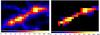 |
Fig. 1 Gas density (1010 M⊙ Mpc-3) image of an interesting region from the simulation (C12) when applying no filtering (left panel) and when applying the filamentary environment selection (right panel). The pixel size and the image thickness are both 1.4 Mpc. |
3.3. Application of filament-finding and LD field methods to simulated data
We constructed the r band luminosity density (LDr) fields by applying the LD method to the galaxy population created above. We first extracted the luminosity densities and gas densities in the full volume of the simulation studied in this work. We found that the fraction of the gas mass in the WHIM temperature and density range, i.e. the WHIM volume filling factor, is ~50%.
We then applied the Bisous model to the galaxy distribution and defined volume elements with visit parameter values higher than 0.005 (see Sect. 2.1) as members of filaments. The benefit of this procedure is that it can be applied to both simulated and observational data, based only on the 3D distribution of the galaxies. However, in the case of the observational data, we do not have any temperature or density information for the studied intergalactic gas. As a consequence, for consistency, we do not apply any temperature or density selection directly when extracting the simulated data.
The environmental selection did, in fact, have the desired effects of excluding the voids and the noisy, low temperature filament edges and concentrating more on the filament cores (see Fig. 1). The WHIM mass fraction increased from 50% to 70% when we restricted the analysis to this environmentally selected volume. Below, we thus assume that 70% of the gas mass in the regions that satisfy the Bisous model filament detection criteria is WHIM, i.e. ρwhim = 0.7 × ρgas.
We decided to exclude galaxy clusters from the analysis because their high galaxy number density and low expected WHIM mass fraction (e.g. Branchini et al. 2009) yields a very different LD-WHIM density ratio from that in the filaments. The above filtering rather efficiently reduces the contribution of clusters of galaxies, which is proved by the fact that only ~10% of the selected gas mass has a temperature and densities that both exceed the WHIM upper limits.
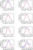 |
Fig. 2 WHIM density distributions (crosses) and the best-fit log-normal models (lines) within selected LD bins. δLD indicates the central luminosity overdensity value of a given bin. δwhim indicates the WHIM overdensity value corresponding to the peak value. |
3.4. Determining the probability distribution function of the WHIM density in different luminosity environments
The relation between the WHIM density and the luminosity density, which are both stochastic tracers of the underlying mass density field is, unsurprisingly, also stochastic. As a result, for a given LDr the values of the WHIM density cover quite a broad range. Here we want to quantify more than the simple spread: we characterise the constrained probability function P(ρwhim | LDr).
We restricted our analysis to the LDr range of [0.01−2.0] × 1010 L⊙ Mpc-3. This choice is justified on the basis of the simulations of (C12) that indicate that ~95% of the WHIM mass of the full simulation volume is within this LDr range. Increasing the range would, therefore, decrease the purity of the sample. We divided this LDr range into 15 equally-spaced logarithmic bins and measured the conditional PDF in each of them.
The frequency histograms of the WHIM gas density at a given LDr bin constitute our estimate of the conditional probability distribution function P(ρwhim|LDr) (see Fig. 2). The WHIM density value corresponding to the position of the maximum correlates with the LDr value, which indicates the presence of an LD–WHIM density correlation that we explore in the next section. As long as LDr is small, the PDF is well approximated by a log-normal distribution. For δLD> 10 a positive skewness appears that develops into a secondary peak at δwhim ~ 30. This shifts to progressively higher ρwhim values as LD increases. These features suggest the presence of a population of luminous objects with associated WHIM gas with overdensities higher than ~10. We speculate that these objects correspond to luminous galaxies or groups with relatively dense WHIM gas in their X-ray halos. The WHIM gas associated with this peak seems to follow the same LD–WHIM density relation as the gas in the main peak indicates that this is a real feature and not a simulation artefact.
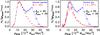 |
Fig. 3 WHIM density distribution at δLD ~ 65 (where the WHIM density peaks at δb ~ 26) using all the simulation data within the filamentary environments are shown with blue crosses and dashed lines. Red crosses indicate the distribution when using only volume elements with galaxies fainter than Mr = −20.5 (left panel), or with gas hotter than T = 5 × 10⁶ K (right panel). |
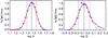 |
Fig. 4 Distributions (blue crosses) of the power-law |
To test this hypothesis we went back to the simulations to characterise mock galaxies and the gas that contribute to the secondary peaks. We found that the peak disappeared when we removed the data from volume elements with galaxies brighter than Mr = −20.5 or gas colder than T = 5 × 10⁶ K from the sample (see Fig. 3). This indicates that the second peak is contributed by gas particles that are usually associated with bright galaxies found in halos with masses in excess of a few times 1012 M⊙ (see Appendix A). These objects are rarely isolated and, instead, are typically found in groups (see Appendix A). Taking the relatively low temperature into consideration as well, the secondary peak, thus appears to be contributed by gas halos of galaxies within galaxy groups or by the intra-group gas, or both.
3.5. LD – WHIM density relation
Within the filamentary environments, the simulated WHIM density and the LDr correlate well: the Pearson correlation coefficient is ~0.80, while the number of data points is ~1.7 × 10⁶. This indicates that the LD traces the WHIM effectively. Consequently, we have used this correlation to find the WHIM in what follows.
We achieved our main goal of estimating the relation between LD and WHIM gas density as follows. 1) We considered the conditional probability functions P(ρwhim | LDr) in each one of the 15 LDr bins. 2) We used the Monte Carlo method when sampling the individual PDFs to obtain a statistical realisation of the LDr−ρwhim relation. 3) We fitted the corresponding data with a power-law relation  and stored the best fit parameters A and B. 4) We went back to Step 1 and repeated the procedure 104 times. 5) We estimated the resulting PDFs for A and B.
For both parameters, the PDF was approximated well by a log-normal distribution except in the positive tail, where the B parameters exhibit an excess probability (see Fig. 4). Using the centroids and the widths of the best-fit log-normal models to the distributions we thus obtained the LDr−ρwhim relation as  (1)and an analogous one expressed in terms of gas overdensity
  (2)where the luminosity overdensity, δLD = LD/⟨LD⟩, is the independent variable, δwhim = ρwhim/⟨ρb⟩, and ⟨ρb⟩ = 0.62 × 10¹⁰ M⊙ Mpc-3 at z = 0 (Planck Collaboration XIII 2015).
The parameter uncertainties in Eqs. (1)and (2)reflect the scatter among the power-law fits to the different Monte Carlo realisations, which is Gaussian if we consider the logarithm of the quantities. We estimated the parameter uncertainties assuming that A and B are fully independent. This assumption is probably not fully valid, and thus the parameter uncertainties are only approximate. While the normalisation parameter A is formally constrained within 20%, the correlation between A and B (the higher normalisation may be compensated for by a steeper slope to some extent) is expected to yield larger variations for the WHIM density at given LD. To include the parameter correlations in the error propagation, we used the power-law fits of Step 3 above: at each LD value we calculated the 68% confidence intervals for the WHIM density using the variation given by the different best-fit pairs of A and B values. In the range δb ~ 10−100, the WHIM density is uncertain by a factor of 2–3, while at the lower densities (δb ~ 1−10), the variation reaches a factor of ~10 (see Fig. 5).
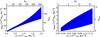 |
Fig. 5 Power-law approximation of the relation between the luminosity density (LDr) and the WHIM density (ρwhim) within the galaxy filaments in the simulations of C12 (solid line), and the 1σ uncertainty interval (blue region). The left-hand panel shows the full fitted LD range and the right-hand panel shows the δb ~ 1−10 range. |
4. Testing the method
In our current work, the emphasis has been on a detailed description of our WHIM method. In a follow-up paper we will carry out a full test of the reliability of our method, using all available data of sufficient quality. Here we perform a first test on the accuracy of our LD-based WHIM column density predictions by comparing them with those obtained independently via X-ray absorption measurements of a background blazar.
We chose to apply the first test to the Sculptor Wall (SW) and Pisces-Cetus (PC) superclusters, in the sight line to the background blazar H2356-309, since 1) they are among the closest reported X-ray absorption systems (z ~ 0.03 and ~0.06), respectively (F10 and Z10); 2) they are covered by galaxy survey data of sufficient quality (2dF, see Colless et al. 2001; Tago et al. 2006); and 3) their reported WHIM column densities are among the highest in the literature.
4.1. Luminosity density fields and galactic filaments
We applied the LD method (see Sect. 2.2) to the bj band luminosities of the galaxies around SW and PC (see Fig. 6) and thus produced the LDbj fields (see Fig. 7). Close to the redshifts of the X-ray absorption line centroids of both SW and PC, the blazar sight line passes through enhanced LD regions (see Fig. 7). The enhancement of LD at the locations of the X-ray detected WHIM supports our finding from the simulations (C12) that LD traces the WHIM.
We then applied the Bisous model (see Sect. 2.1) to the above galaxy distribution to identify galactic filaments. We found that there are several filaments within the enhanced LD regions (see Fig. 6). There are 247 galaxies that affect the LD profiles of SW and PC, i.e. they are located within two times the size of the LD field smoothing kernel (2.8 Mpc) from the H2356-309 sight line at the matching redshifts. Only two of these were classified as non-filament galaxies. This supports our finding from simulations (C12) that within the filamentary environments, the WHIM density is enhanced from the cosmic average. Thus, it is justified to apply below the LD-WHIM density relation (Eq. (2)), derived within the filamentary environments.
Since both absorbers have originally been targeted because of a priori knowledge of the large-scale concentrations of galaxies around them, the above agreement serves as a positive indicator of the performance of our filament finder. We will perform a more robust test in subsequent work.
The fortuitous combination of the blazar position and the orientation of the filaments in both SW and PC results in relatively long (~10 Mpc) line of sight projection of high LD regions. This contributes to these systems being among the most significant WHIM structures detected by X-rays to date.
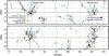 |
Fig. 6 Spatial distribution of 2dF galaxies around the H2356-309 sight line (yellow line) projected at two orthogonal directions (upper and lower panels) at the distance range covering SW and PC structures. The coordinates refer to the CMB rest frame. The galaxies belonging to filamentary environments are denoted with plus signs, while other galaxies are denoted with crosses. The filament spines are indicated with green lines. The relative LD level at each radii is denoted with the blue line. The red parts of the sight line highlight the radial ranges of the luminosity density profiles analysed in this work (see Fig. 8). |
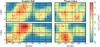 |
Fig. 7 2dF bj band luminosity density field slices of 1.4 Mpc thickness in two orthogonal directions (upper and lower panels) along the line of sight towards the blazar H2356-309 (red horizontal lines) in the SW (left panels) and PC (right panels) structures. The contours indicate our adopted lower LD threshold LDbj,min = 0.05 × 10¹⁰ L⊙ Mpc-3 for extracting the data for further analysis. The radial ranges equal those used for the luminosity density profile analysis (see Fig. 8). The galaxies relevant to the sight line, i.e. within a distance of two times the smoothing kernel size from the sight line (2.8 Mpc), are marked with dark red symbols: plus signs correspond to locations of galaxies belonging to a filamentary environment while other galaxies are denoted with crosses. The purple vertical lines indicate the centroids of the Chandra X-ray absorption lines (F10; Z10). |
4.2. Luminosity-density profiles and NH
To evaluate the column densities along the sight line, we proceeded by characterising the radial behaviour of the luminosity density. We performed this by producing the LDbj profiles of SW and PC by sampling the LDbj fields along the line of sight towards the blazar H2356-309 (see Fig. 8). By examining the LD fields and the LD profiles (see Figs. 7 and 8), we set a lower LD threshold LDbj,min = 0.05 × 10¹⁰ L⊙ Mpc-3 to consider the radial profile of the LD field across the X-ray line centroid, and set the likely redshift range (z1−z2) of the absorber equal to that in which LDbj> LDbj,min.
Within the reported uncertainty range of the redshift of the X-ray absorber (F10; Z10), there is a continuous, two-peaked structure of ~10 Mpc length in both SW and PC (see Fig. 8). The redshifts of the two peaks in the LD profiles are very similar. Their separation, Δz ~ 0.001, corresponding to ΔΛ ~ 0.01 Å, at 20 Å, is below the energy resolution of both Chandra/LETGS and XMM-Newton/RGS. Therefore we considered the full ~10 Mpc long two-peaked structure as a single system for both SW and PC.
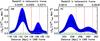 |
Fig. 8 2dF bj band luminosity density profiles of the SW (left panel) and PC (right panel) along the H2356-309 sight line (solid black lines) together with 1σ uncertainties (blue regions). The horizontal (green dashed line) indicates our adopted lower LD threshold LDbj,min = 0.05 × 10¹⁰L⊙ Mpc-3 for extracting the data for further analysis. The vertical dashed lines indicate the best-fit heliocentric redshifts of the Chandra X-ray lines, while the dotted lines bracket the statistical 1σ uncertainties of the redshifts (from F10 and Z10). The co-moving distances refer to the CMB rest frame. |
We then converted our measured bj band LD profiles into units of luminosity overdensities δLD(z) = LDbj(z)/⟨LDbj⟩ (see the discussion in Sect. 3.2) by applying the mean bj band luminosity density in the full 2dF survey (see Table 1). We then used our LD–WHIM density relation (Eq. (2)) to convert the above luminosity overdensity profiles into WHIM density profiles. Integration of the density profile then yielded the column density estimates using  (3)
(3)
4.3. Uncertainties of the estimated WHIM column densities
In this section we analyse the two main sources of uncertainties affecting the estimates of the WHIM column densities. First, we analyse the reliability of the observed luminosity density profiles. Second, we analyse the effect of the scatter in the calibration of the LD–WHIM density relation in simulations (C12).
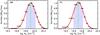 |
Fig. 9 WHIM hydrogen column density distributions (black crosses), an effect of the LD profile measurement uncertainties for the SW (left panel) and PC (right panel) structures. The best-fit log-normal models are shown with solid red lines. The best value and the 1σ confidence intervals are indicated with dashed green lines and shaded blue regions, respectively. |
4.3.1. Uncertainties of the observed luminosity density field
The main source of uncertainty in an observed LD profile is the shot noise due to the limited number of galaxies used for the LD field construction. We estimated this effect by applying a smoothed bootstrap procedure on the 2dF galaxy sample (see Liivamägi et al. 2012, for more details and justification of the use of the smoothed bootstrap in this context). Briefly, we removed a random galaxy, and randomised the positions and the redshifts of the other galaxies, and evaluated the LD profile. The distance between the randomised position and the original one is defined by a smoothing kernel, which is half the size of the original LD field-smoothing in Sect. 2.2. Repeating this procedure 10 000 times, we obtained a set of bootstrapped LD profiles for SW and PC, and we used the 68% LD scatter interval at each radius to determine the uncertainties of the LD profile measurements (see Fig. 8).
We propagated this scatter into NH measurement by converting each bootstrapped LD profile into a WHIM density profile using Eq. (2)and integrating the profiles using Eq. (3). The resulting NH distributions followed the log-normal prediction well (see Fig. 9). We thus used the best-fit log-normal centroid and width parameters to obtain the best values and 1σ intervals of NH: 0.8 [0.6–1.1] × 1020 cm-2 and 0.5 [0.4–0.7] × 1020 cm-2 for SW and PC, respectively.
4.3.2. Effect of scatter in the LD-WHIM density relation
Owing to the significant scatter of the WHIM density values for a given LD value in the cosmological simulations used in this work, our model prediction is statistical by nature. The following list contains a brief discussion about the possible origins of the scatter:
-
The galaxy luminosity and the WHIM density do not solely depend on the underlying DM density but may depend on, for example, the stellar feedback mechanisms and the gas physics.
-
The HOD used to populate the dark matter halos with galaxies is statistical by nature.
-
The DM halo geometry may deviate from the assumed spherical symmetry in the HOD modelling.
We have already characterised this scatter in Sect. 3.5 by the power-law fits to the set of randomised LD-WHIM density relations, when deriving the uncertainties of the LD-WHIM density power-law model parameters. Because of the parameter correlations (see Sect. 3.5), we did not perform a simple analytical error propagation using Eqs. (2)and (3). Rather, we used the pairs of the best-fit power-law normalisation and index parameters obtained in Sect. 3.5 here to obtain a set of LD-WHIM density relations that reflects the scatter of the WHIM density values for a given LD in C12 simulations. We applied each of these scattered LD-WHIM density relations to the measured LD profiles of SW and PC first to obtain a set of WHIM density profiles, and then by integration, we obtained distributions of NH values for both structures (see Fig. 10).
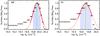 |
Fig. 10 WHIM hydrogen column density distributions (black crosses) resulting from the LD–WHIM density scatter in the simulations (C12) for the SW (left panel) and PC (right panel) structures. The best-fit log-normal models (red lines) in the fitted range (solid line) are shown together with the extrapolation (dotted line). The best value and the 1σ confidence intervals are indicated with dashed green lines and the blue shaded regions, respectively. |
At NH values within the 68% confidence interval around the centroid, the distributions can be approximated reasonably well with a log-normal model. We thus used the best-fit log-normal centroid and width parameters to obtain the best values and 1σ intervals of 0.8 [0.6–1.1] × 1020 cm-2 and 0.5 [0.4–0.8] × 1020 cm-2 for the NH in SW and PC, respectively. At the lowest and the highest NH values, the distribution significantly exceeds the log-normal distribution. The low-end tail is a consequence of the high-end tail of the index distribution (see Fig. 4). The rather large (by a factor of ~10) uncertainty of the LD-WHIM density relation at the lowest densities (see Fig. 5) has a negligible effect in the case of SW and PC, since most of the measured LD values are much higher (see Fig. 8).
Properties of the absorbers.
4.4. Final NH values
The effects of 1) the SW LD profile measurement uncertainties, using the 2dF data; and 2) the LD-WHIM density scatter in the cosmological simulations, on the NH estimates are similar and significant (i.e. a variation by a factor of ~2). We thus combined the two uncertainties in quadrature. The best values differ slightly, so we averaged them, obtaining the final results that are given in Table 2.
4.5. Comparison with X-rays
Our procedure predicts the hydrogen column density of the WHIM from the galaxy luminosity density. However, the typical signatures of the WHIM in the X-ray band are line features from highly ionised metals, such as O vii. The conversion between the hydrogen column density and metal ion column density depends on the ionisation fraction (i.e. the temperature) and the metal abundance. If only a single absorption line is measured, as in the case of the SW structure (F10), the temperature and column density constraints are very poor. If we assume that oxygen abundance is 0.1 solar and that the temperature is 106 K (i.e. the ionisation fraction of O vii is 1.0) our NH estimate for the SW structure ( ) translates to
  , consistent within the large uncertainties of the X-ray measurement of F10,
  (see Table 2).
In the case of the PC structure, lines from several elements and ionisation stages were reported (Z10) for a warm absorber2 (log T (K) ~ 5.4). Thus the temperature and the equivalent hydrogen column density were well constrained and we can make a direct comparison (assuming that oxygen abundance is 0.1 solar). Our estimate ( ) is consistent within 1σ uncertainties with that of Z10, i.e. log NH = 20.1 ± 0.2.
The agreement of our LD-based prediction for the column density of the WHIM in SW and PC structures with that obtained from X-ray absorption measurements indicates that our method is robust. This also indicates that the luminosity density and the galactic filaments are reliable signposts for the WHIM.
5. Galaxy confusion
In the above we interpreted the X-ray absorption features being due to WHIM. We examine here an alternative hypothesis, namely galaxy confusion, which states that instead of the intergalactic diffuse WHIM, the absorption is caused by the X-ray halos of accidental galaxies close to the studied sight line (e.g. Williams et al. 2013). In this case the match of our intergalactic LD-based WHIM column densities and the X-ray ones (F10; Z10) is not causal, but rather a coincidence.
Nearby galaxies.
The sole existence of a galaxy within a virial radius from an X-ray absorber is obviously no proof that the galaxy and its circum-galactic gas are the cause of the X-ray absorption features that we consider WHIM signatures. We explore the galaxy confusion hypothesis quantitatively in this work by: 1) estimating the density of the X-ray halos of the nearby galaxies at the distance of H2356-309 sight line; and 2) comparing these estimates with the X-ray measurements. As possible candidates we very generously considered all such 2dF galaxies within the redshift range, matching those of the SW and PC structures that are located within 1 Mpc (i.e. several times the virial radii) from the H2356-309 sight line. There are eight (five) of such candidates for the SW (PC), (see Table 3).
In the above list, there are no massive galaxies, i.e. obvious candidates for galaxy confusion. It is possible that close to the sight line there are galaxies fainter than the 2dF limit, corresponding to MB ~ −16 at these redshifts. However, these luminosities correspond to ~1% of that of the Milky Way. Thus, it takes 100 of these objects to reach the mass of the Milky Way and possibly a similar WHIM NH level of 1019 cm-3 (assuming the temperatures of the halos do reach WHIM values). These objects need to be clustered at the sight line, at the redshifts consistent with the X-ray measurements. Thus these objects should be more clustered than the Milky Way-like galaxies, (see Table 3), meaning that their bias parameter should be larger. This is inconsistent with observations and simulations that show that faint galaxies are less clustered than luminous ones (e.g. Norberg et al. 2002a; C12).
Galaxy 3, in our list, is the only elliptical galaxy while all others are spiral. In the following we examine these two galaxy types separately. For a comparison with other works on galaxies, we approximated the absolute bj band magnitudes and luminosities with those in the B band (Norberg et al. 2002b).
5.1. Elliptical galaxy 3
Williams et al. (2013) suggest that the elliptical galaxy 3 in our list, at a distance of 240 kpc from the H2356-309 sight line at the redshift of the SW, may be responsible for the X-ray absorption measured by F10. The bj band magnitude of the galaxy corresponds to LB ~ 1010LB ⊙. From the analysis of X-ray halos of elliptical galaxies (Fukazawa et al. 2006), the corresponding X-ray luminosity of this object would be LX ~ 1040 erg s-1 and a temperature of T ~ 106 K, consistent with WHIM properties. Extrapolating the corresponding gas density profile in (Fukazawa et al. 2006) to a radius of 240 kpc (corresponding to the impact parameter of the sight line to H2356-309) yields a density level of ~10-5 cm-3. With such a low density, a path length of ~1025 cm, i.e. ~10 Mpc, would be required to build up the measured level of the column density, i.e. NH ~ 1020 cm-2. This is clearly inconsistent with the virial radius of the galaxy, estimated as 350 kpc in Williams et al. (2013).
5.2. Spirals
All the spiral galaxies in the candidate list have a much lower or similar B-band luminosity LB compared to the Milky Way, whose MB ≈ Mbj ~ −20 (Binney & Merrifield 1998; Pritchet & van den Bergh 1999; van den Bergh 2000). We use the LB values for comparing the stellar masses of the candidate spirals with that of the Milky Way. This is complicated since the B band may be contaminated due to star formation. All our candidate spirals are star-forming, so they probably have a similar bias in the B-band-based mass estimates of the candidates and the Milky Way. However, to form a conservative estimate, we assumed a factor of 100 scatter in the mass/LB ratio, rendering the most massive candidate spirals 100 times more massive than the Milky Way.
The intensity of the X-ray emission from T ~ 106 K gas in several edge-on spiral galaxies (e.g. NGC 5775 Li et al. 2008 and NGC 4631 Yamasaki et al. 2009) has been observed to decrease exponentially with the distance from the galactic plane. The joint X-ray emission and absorption measurements of O vii and O viii lines of the Milky Way halo have obtained temperatures ~106 K (consistent with WHIM) and equivalent hydrogen column densities at 1019 cm-2 level (e.g. Hagihara et al. 2010; Sakai et al. 2014), i.e. ~10% of what is consistently determined by us and via X-rays in SW and PC. The resulting path length scale of the absorber, and thus the extent of the WHIM halo in spiral galaxies in the above works, is consistently constrained below 10 kpc. While this indicates that the halo is identified with the stellar component, this also conflicts with the reports of the extent of ~100 kpc of the WHIM halo in the Milky Way (e.g. Gupta et al. 2012). In fact, Wang & Yao (2012) report numerous significant errors in Gupta et al. (2012), which resulted in an order of magnitude overestimation of the Galactic WHIM halo size.
Since our candidate spirals have masses less than 100 times that of the Milky Way (see above), we make a conservative estimation that all our candidate spirals have WHIM halos with a similar exponentially decreasing density profile to that of the Milky Way, but scaled up by a factor of 100, i.e. with a central density of 10-1 cm-2 and a scale height of 3 kpc. The most likely candidate for galaxy confusion is Galaxy 9 (see Table 3), the one nearest to the absorbers. Williams et al. (2013) associate this galaxy with the X-ray absorber at PC (Z10). Extrapolating the exponential density profile to 50 kpc (the distance between the galaxy and H2356-309 sight line), we obtain a very low WHIM density of 10-8 cm-3. Let’s assume that the column density of ~1020 cm-2 is achieved along an absorber path length of 10 kpc (~1022 cm). Consequently, the required number density of the WHIM halo is ~10-2 cm-3 at the distance of the H2356-309 sight line from the centre of a given galaxy. Thus, the exponential density profile of Galaxy 9 totally fails to produce the measured level of WHIM column density. Since the other galaxies are more distant, the discrepancy is even bigger for those. Unless we underestimated the candidate spiral to Milky Way mass ratio by a factor of 106, as a result of the star formation issue, the candidate spirals cannot produce the measured absorption in PC.
In general, when considering the projection effects, it is necessary for a Milky Way-like galaxy to be located within ~10 kpc to the blazar sight line to produce WHIM column densities at a level of ~1019 cm-2.
6. Discussion
In this work, we have tested the ability of our method to infer the presence of the WHIM by targeting large-scale structures associated with putative WHIM detections. In the future, we shall apply our method to perform a blind WHIM search along sight lines to distant quasars, located within the areas of the 2dF and SDSS galaxy surveys. Our method is not limited to being directed towards the brightest background blazars, as is the case for the current rare WHIM detections that are based on identifying characteristic X-ray and far ultraviolet absorption lines. Rather, our method has potential to extend the hunt for the missing baryons to the full volumes of the spectroscopic galaxy surveys, such as SDSS and 2dF.
Our method can be used to estimate the mass density of the WHIM. Combined with the independent X-ray or FUV absorption measurements of the same WHIM structures, our additional constraint has the potential to improve the diagnostics of WHIM physics. In particular, there is a possibility of breaking the degeneracy between the WHIM column density and the abundance of the absorbing metal, thus providing constraints for the latter. This could improve our understanding of the chemical and thermal enrichment of the intergalactic medium via supernovae explosions and AGN feedback. Currently these effects are poorly understood and modelled in the hydrodynamical simulations.
Our LD–WHIM density relation, used together with the filament-tracing technique, has potential for mapping a large sample of WHIM properties with current data. This is necessary for properly assessing the contribution of WHIM to the cosmological mass density budget. Thus our method has the potential to help us understand of the problem of cosmological missing baryons in the near future. Our methods and the potential WHIM maps could be used to optimise the observational strategies in searching for the missing baryons with next-generation satellites, like Athena.
7. Conclusions
In this work we proposed, implemented, applied, and tested a novel method of identifying the elusive WHIM, studying galaxies in the filaments of the cosmic web. Our method rests upon a correlation between the density of the “invisible” WHIM and that of the observed galaxy luminosity. The calibration of the method was performed using the hydrodynamical numerical simulation (C12) and HOD-based mock galaxy catalogues that mimic the properties of SDSS galaxies, following the prescriptions of Zehavi et al. (2011). To test the performance of our method on observational data, we applied it to the distribution of galaxies in the 2dF survey, focusing on the SW and PC superclusters. The main results, obtained both in the calibration and application phases, are summarised below.
-
In the C12 simulation, the WHIM is usually associated with the filamentary structures. We identified the latter by applying the Bisous model (Stoica et al. 2005; Tempel et al. 2014a) to the distribution of the mock galaxies and found that the mass fraction of the gas in WHIM phase associated to these structures is ~70%, by a factor of ~1.6 higher than the average in the full simulation box.
-
When considering the WHIM gas and the galaxy luminosity in the filament environments, we found a significant correlation between their densities. The Pearson correlation coefficient between the two turned out to be ~80%, and the relation between the WHIM gas overdensity and the galaxy luminosity overdensity consistent with linear δwhim = 0.7 ± 0.1 × δLD0.9 ± 0.2. This suggests that both the diffuse gas in the WHIM and the stellar component in the galaxies trace the same underlying DM density field.
-
The above relation can be used in reverse, i.e. given the observed luminosity density in the filamentary structures that have been identified in the spatial distribution of galaxies in galaxy redshift surveys, one can use the relation to infer the column density of the WHIM.
-
When testing our method on observational data, we found that the luminosity density was significantly enhanced from the average at the locations of independently detected WHIM (F10; Z10). This indicates that the luminosity density traces the WHIM, which is consistent with our findings in the simulations.
-
Our LD-based predictions for the column density of the WHIM in the SW and PC superclusters agree with those obtained via X-ray absorption. This agreement indicates that our method is robust in estimating the density of WHIM. Also, the galaxy filaments and the luminosity density are reliable signposts of WHIM.
-
The signal that we detected cannot originate in the halos of nearby galaxies since they cannot account for the high WHIM column densities that our method and X-ray analysis consistently find in the SW and PC superclusters.
-
The fortuitous combination of the angular position of the bright background blazar H2356-309 behind suitably oriented, long filaments in the SW and PC superclusters results in relatively long (~10 Mpc) line-of-sight projections of high LD regions. This contributes to these systems being among WHIM structures with the most significant X-ray detections to date.
Online material
Appendix A: HOD formalism
We applied halo occupation distribution (HOD) formalism to our adopted large-scale simulation of Cui et al. (2012) to construct the galaxy distribution. DM halos and subhalos represent tracers of the central galaxies and satellites, respectively (Peacock & Smith 2000; Kravtsov et al. 2004; van den Bosch et al. 2007). We thus started by producing a DM halo catalogue by applying the friend-of-friend (FoF) algorithm with linking length parameter b = 0.2 (in the units of the mean inter-particle separation) to the simulated data. This choice of the linking length value yields mass functions consistent with different theoretical predictions of the virial mass function (e.g. Gao et al. 2004; Springel 2005). The resulting FoF catalogue contains the position and the virial mass of each DM halo. In the following we describe how we used the FoF catalogue to obtain the magnitudes and positions of the galaxies.
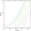 |
Fig. A.1 Halo occupation number, i.e. the mean number of galaxies in a halo of a given virial mass, is shown in different luminosity bins (colour coding as in Fig. A.3). The solid histograms represent the statistical realisations of the galaxies that populate the halos extracted from the (C12) simulation and their substructures. The dotted curve shows the predictions from Eq. (A.2) using the parameters in Zehavi et al. (2011). |
-
1.
For each DM halo we used its FoF mass from above to calculatethe virial radius Rvir, to know up to which scale to populate it with subhalos. This was done according to the spherical collapse formalism that yields the estimate of the virial overdensity Δvir(z) (e.g. Peebles 1980; Eke et al. 1996; Kitayama & Suto 1996; Bryan & Norman 1998). This is linked to the virial mass and the virial radius as
 (A.1)where ρc(z) and Ωm(z) represent the critical density and the cosmological matter density parameter at redshift z, respectively.
 -
2.
We assigned each halo a concentration parameter according to mass-concentration relation of Bullock et al. (2001), assuming a log-normal scatter σlnc = 0.25 around the mean value.
-
3.
We populated each halo with subhalos by performing Monte Carlo realisations of the subhalo mass function model of Giocoli et al. (2010), which features both a redshift evolution and a concentration dependence on the subhalo mass function. The model assumes that the spatial distribution of the subhalos is less concentrated than the NFW DM profile (Navarro et al. 1996), since this includes the effects of dynamical friction and tidal stripping (Gao et al. 2004; van den Bosch et al. 2004; Giocoli et al. 2008). Accordingly, for each halo we now have subhalo populations with known positions and masses.
-
We then assigned each halo and subhalo with a galaxy with a luminosity value according to the abundance-matching approach (see e.g. Behroozi et al. 2010) as follows. At the core of the method is the halo occupation function
![\appendix \setcounter{section}{1} \begin{eqnarray} \langle N(M_{\rm h}) \rangle = \frac{1}{2} \left[1 + \mathrm{erf} \left( \frac{\log M_{\rm h} - \log M_\mathrm{min}}{\sigma_{\log M}} \right) \right] \nonumber \\ \times \left[1 + \left( \frac{M_{\rm h} - M_0}{M'_1}\right)^{\alpha} \right] , \label{eqhod} \end{eqnarray}](/articles/aa/full_html/2015/11/aa26443-15/aa26443-15-eq172.png) (A.2)which describes the mean number of halos within a parent halo of mass Mh (Zehavi et al. 2011).
(A.2)which describes the mean number of halos within a parent halo of mass Mh (Zehavi et al. 2011). 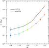
Fig. A.2 Median masses of parent halos (solid line and crosses) and subhalos (dotted line and dots), derived in Sect. 3.2, hosting galaxies with different r-band absolute magnitudes, when applying the HOD formalism to C12 simulations (colour coding as in Fig. A.3).
We then made the standard assumptions that: 1) all subhalos are populated by one galaxy only, i.e. the number of substructures into which we have resolved the parent halos is sufficient to host at most one galaxy; and 2) there are no “orphan” subhalos. The latter hypothesis is justified by the lack of evidence for massive dark halos with no baryon content. Based on these assumptions, Eq. (A.2)then describes the mean number of galaxies within a parent halo of mass Mh. The values of the parameters of Eq. (A.2)were found by Zehavi et al. (2011) by fitting the projected SDSS-DR7 2-point galaxy-galaxy correlation function of Abazajian et al. (2009) in the luminosity range Mr = −[18.5,22] , sampled in seven, equally spaced, bins. Consequently, the parameters of Eq. (A.2)are different for each luminosity bin. We then applied the method to our FoF DM halos obtained from the C12 simulations as follows: for a given parent halo of mass Mh, we use Eq. (A.2)to determine the mean number of galaxies at a given magnitude Mr (see Figs. A.1 and A.2). We repeated the procedure for each magnitude bin from Mr = −18.5 to Mr = −22, thus obtaining the luminosity function N(Lr) for a given host halo.
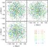
Fig. A.3 Three orthogonal projections of the distribution of satellite galaxies in centres of DM halos of ~1 Mpc radius in our adopted simulation of C12 (coloured dots). The colour coding indicates the magnitude of a given galaxy. The black dots show the positions of galaxies fainter than Mr = −18 that populate halo and subhalos in the simulation according to the mass function by Giocoli et al. (2010) down to 1010 M⊙.
We then ranked the above galaxies from most luminous to least luminous. For the same parent halo we went back to the subhalo distribution obtained above (Giocoli et al. 2010) and ranked the subhalos from most massive to least massive. We then matched the parent halo or its subhalo of a given mass ranking to a galaxy with the same luminosity ranking (most massive with the most luminous etc.) until all galaxies were assigned to the subhalos. We removed the low mass subhalos that were assigned to no galaxies. The outcome is a set of parent halos, extracted from the C21 simulation, containing a set of subhalos. Each halo and subhalo has a galaxy at its centre with known location and r-band luminosity (see Fig. A.3).
Z10 also reported a possible hotter component at the same redshifts. However, because of its lower significance, we do not consider it here.
Acknowledgments
J.N. is funded by PUT246 grant from the Estonian Research Council. We acknowledge funding from the ESF grants IUT26-2, IUT40-2 and TK120 (the European Structural Funds grant for the Centre of Excellence “Dark Matter in (Astro) particle Physics and Cosmology”). Thanks to F. Pace for providing mapping routines. Thanks to P. Teenjes and M. Einasto for help. E.B. acknowledges the financial support provided by MIUR PRIN 2011 “The dark Universe and the cosmic evolution of baryons: from current surveys to Euclid” and Agenzia Spaziale Italiana for financial support from the agreement ASI/INAF/I/023/12/0. We thank S. Borgani and G. Murante for giving us access to the simulations analysed in this paper. C.G. thanks CNES for financial support.
References
- Abazajian, K. N., Adelman-McCarthy, J. K., Agüeros, M. A., et al. 2009, ApJS, 182, 543 [NASA ADS] [CrossRef] [Google Scholar]
- Baugh, C. M. 2013, PASA, 30, 30 [Google Scholar]
- Behroozi, P. S., Conroy, C., & Wechsler, R. H. 2010, ApJ, 717, 379 [NASA ADS] [CrossRef] [Google Scholar]
- Binney, J., & Merrifield, M. 1998, Galactic Astronomy (Princeton University Press) [Google Scholar]
- Branchini, E., Ursino, E., Corsi, A., et al. 2009, ApJ, 697, 328 [NASA ADS] [CrossRef] [Google Scholar]
- Bregman, J. N. 2007, ARA&A, 45, 221 [NASA ADS] [CrossRef] [Google Scholar]
- Bryan, G. L., & Norman, M. L. 1998, ApJ, 495, 80 [NASA ADS] [CrossRef] [Google Scholar]
- Bullock, J. S., Kolatt, T. S., Sigad, Y., et al. 2001, MNRAS, 321, 559 [Google Scholar]
- Buote, D. A., Zappacosta, L., Fang, T., et al. 2009, ApJ, 695, 1351 [NASA ADS] [CrossRef] [Google Scholar]
- Cen, R., & Ostriker, J. P. 1999, ApJ, 514, 1 [NASA ADS] [CrossRef] [Google Scholar]
- Cen, R., & Ostriker, J. P. 2006, ApJ, 650, 560 [NASA ADS] [CrossRef] [Google Scholar]
- Colless, M., Dalton, G., Maddox, S., et al. 2001, MNRAS, 328, 1039 [NASA ADS] [CrossRef] [Google Scholar]
- Cui, W., Borgani, S., Dolag, K., Murante, G., & Tornatore, L. 2012, MNRAS, 423, 2279 [NASA ADS] [CrossRef] [Google Scholar]
- Davé, R., Cen, R., Ostriker, J. P., et al. 2001, ApJ, 552, 473 [NASA ADS] [CrossRef] [Google Scholar]
- Eke, V. R., Cole, S., & Frenk, C. S. 1996, MNRAS, 282, 263 [NASA ADS] [CrossRef] [Google Scholar]
- Fang, T., Buote, D. A., Humphrey, P. J., et al. 2010, ApJ, 714, 1715 [NASA ADS] [CrossRef] [Google Scholar]
- Fukazawa, Y., Botoya-Nonesa, J. G., Pu, J., Ohto, A., & Kawano, N. 2006, ApJ, 636, 698 [NASA ADS] [CrossRef] [Google Scholar]
- Gao, L., White, S. D. M., Jenkins, A., Stoehr, F., & Springel, V. 2004, MNRAS, 355, 819 [NASA ADS] [CrossRef] [Google Scholar]
- Giocoli, C., Tormen, G., & van den Bosch, F. C. 2008, MNRAS, 386, 2135 [NASA ADS] [CrossRef] [Google Scholar]
- Giocoli, C., Tormen, G., Sheth, R. K., & van den Bosch, F. C. 2010, MNRAS, 404, 502 [NASA ADS] [Google Scholar]
- Grevesse, N., & Sauval, A. J. 1998, Space Sci. Rev., 85, 161 [NASA ADS] [CrossRef] [Google Scholar]
- Gupta, A., Mathur, S., Krongold, Y., Nicastro, F., & Galeazzi, M. 2012, ApJ, 756, L8 [NASA ADS] [CrossRef] [Google Scholar]
- Hagihara, T., Yao, Y., Yamasaki, N. Y., et al. 2010, PASJ, 62, 723 [NASA ADS] [Google Scholar]
- Kitayama, T., & Suto, Y. 1996, MNRAS, 280, 638 [NASA ADS] [Google Scholar]
- Kravtsov, A. V., Berlind, A. A., Wechsler, R. H., et al. 2004, ApJ, 609, 35 [NASA ADS] [CrossRef] [Google Scholar]
- Kull, A., & Böhringer, H. 1999, A&A, 341, 23 [NASA ADS] [Google Scholar]
- Li, J.-T., Li, Z., Wang, Q. D., Irwin, J. A., & Rossa, J. 2008, MNRAS, 390, 59 [NASA ADS] [CrossRef] [Google Scholar]
- Liivamägi, L. J., Tempel, E., & Saar, E. 2012, A&A, 539, A80 [NASA ADS] [CrossRef] [EDP Sciences] [Google Scholar]
- Madgwick, D. S., Lahav, O., Baldry, I. K., et al. 2002, MNRAS, 333, 133 [NASA ADS] [CrossRef] [Google Scholar]
- Navarro, J. F., Frenk, C. S., & White, S. D. M. 1996, ApJ, 462, 563 [NASA ADS] [CrossRef] [Google Scholar]
- Nicastro, F., Mathur, S., & Elvis, M. 2008, Science, 319, 55 [NASA ADS] [CrossRef] [Google Scholar]
- Norberg, P., Baugh, C. M., Hawkins, E., et al. 2002a, MNRAS, 332, 827 [NASA ADS] [CrossRef] [Google Scholar]
- Norberg, P., Cole, S., Baugh, C. M., et al. 2002b, MNRAS, 336, 907 [NASA ADS] [CrossRef] [Google Scholar]
- Nusser, A., Davis, M., & Branchini, E. 2014, ApJ, 788, 157 [NASA ADS] [CrossRef] [Google Scholar]
- Peacock, J. A., & Smith, R. E. 2000, MNRAS, 318, 1144 [NASA ADS] [CrossRef] [Google Scholar]
- Peebles, P. J. E. 1980, The large-scale structure of the Universe (Princeton: Princeton University Press), 435 [Google Scholar]
- Planck Collaboration XIII. 2015, A&A, submitted, [arXiv:1502.01589] [Google Scholar]
- Pritchet, C. J., & van den Bergh, S. 1999, AJ, 118, 883 [NASA ADS] [CrossRef] [Google Scholar]
- Ren, B., Fang, T., & Buote, D. A. 2014, ApJ, 782, L6 [NASA ADS] [CrossRef] [Google Scholar]
- Roncarelli, M., Moscardini, L., Tozzi, P., et al. 2006, MNRAS, 368, 74 [NASA ADS] [CrossRef] [Google Scholar]
- Roncarelli, M., Moscardini, L., Borgani, S., & Dolag, K. 2007, MNRAS, 378, 1259 [NASA ADS] [CrossRef] [Google Scholar]
- Roncarelli, M., Cappelluti, N., Borgani, S., Branchini, E., & Moscardini, L. 2012, MNRAS, 424, 1012 [NASA ADS] [CrossRef] [Google Scholar]
- Sakai, K., Yao, Y., Mitsuda, K., et al. 2014, PASJ, 66, 83 [NASA ADS] [Google Scholar]
- Schaye, J., Dalla Vecchia, C., Booth, C. M., et al. 2010, MNRAS, 402, 1536 [Google Scholar]
- Shull, J. M., Penton, S. V., Stocke, J. T., et al. 1998, AJ, 116, 2094 [NASA ADS] [CrossRef] [Google Scholar]
- Shull, J. M., Tumlinson, J., & Giroux, M. L. 2003, ApJ, 594, L107 [NASA ADS] [CrossRef] [Google Scholar]
- Shull, J. M., Smith, B. D., & Danforth, C. W. 2012, ApJ, 759, 23 [NASA ADS] [CrossRef] [Google Scholar]
- Sigad, Y., Branchini, E., & Dekel, A. 2000, ApJ, 540, 62 [NASA ADS] [CrossRef] [Google Scholar]
- Springel, V. 2005, MNRAS, 364, 1105 [NASA ADS] [CrossRef] [Google Scholar]
- Stocke, J. T., Keeney, B. A., Danforth, C. W., et al. 2014, ApJ, 791, 128 [NASA ADS] [CrossRef] [Google Scholar]
- Stoica, R. S., Gregori, P., & Mateu, J. 2005, Stochastic Processes and their Applications, 115, 1860 [Google Scholar]
- Stoica, R. S., Martínez, V. J., & Saar, E. 2007, J. Roy. Stat. Soc. Ser. C, 56, 459 [Google Scholar]
- Stoica, R. S., Martínez, V. J., & Saar, E. 2010, A&A, 510, A38 [NASA ADS] [CrossRef] [EDP Sciences] [Google Scholar]
- Tago, E., Einasto, J., Saar, E., et al. 2006, Astron. Nachr., 327, 365 [NASA ADS] [CrossRef] [Google Scholar]
- Tempel, E. 2011, Ph.D. Thesis, University of Tartu Estonia [Google Scholar]
- Tempel, E., Stoica, R. S., Martínez, V. J., et al. 2014a, MNRAS, 438, 3465 [NASA ADS] [CrossRef] [Google Scholar]
- Tempel, E., Tamm, A., Gramann, M., et al. 2014b, A&A, 566, A1 [NASA ADS] [CrossRef] [EDP Sciences] [Google Scholar]
- Tilton, E. M., Danforth, C. W., Shull, J. M., & Ross, T. L. 2012, ApJ, 759, 112 [NASA ADS] [CrossRef] [Google Scholar]
- van den Bergh, S. 2000, PASP, 112, 529 [NASA ADS] [CrossRef] [Google Scholar]
- van den Bosch, F. C., Norberg, P., Mo, H. J., & Yang, X. 2004, MNRAS, 352, 1302 [NASA ADS] [CrossRef] [Google Scholar]
- van den Bosch, F. C., Yang, X., Mo, H. J., et al. 2007, MNRAS, 376, 841 [NASA ADS] [CrossRef] [Google Scholar]
- Wang, Q. D., & Yao, Y. 2012, ArXiv e-prints [arXiv:1211.4834] [Google Scholar]
- Werner, N., Finoguenov, A., Kaastra, J. S., et al. 2008, A&A, 482, L29 [NASA ADS] [CrossRef] [EDP Sciences] [Google Scholar]
- Williams, R. J., Mulchaey, J. S., & Kollmeier, J. A. 2013, ApJ, 762, L10 [NASA ADS] [CrossRef] [Google Scholar]
- Yamasaki, N. Y., Sato, K., Mitsuishi, I., & Ohashi, T. 2009, PASJ, 61, 291 [NASA ADS] [Google Scholar]
- Zappacosta, L., Maiolino, R., Mannucci, F., Gilli, R., & Schuecker, P. 2005, MNRAS, 357, 929 [NASA ADS] [CrossRef] [Google Scholar]
- Zappacosta, L., Nicastro, F., Maiolino, R., et al. 2010, ApJ, 717, 74 [NASA ADS] [CrossRef] [Google Scholar]
- Zehavi, I., Zheng, Z., Weinberg, D. H., et al. 2011, ApJ, 736, 59 [NASA ADS] [CrossRef] [Google Scholar]
All Tables
All Figures
|
Fig. 1 Gas density (1010 M⊙ Mpc-3) image of an interesting region from the simulation (C12) when applying no filtering (left panel) and when applying the filamentary environment selection (right panel). The pixel size and the image thickness are both 1.4 Mpc. |
| In the text | |
|
Fig. 2 WHIM density distributions (crosses) and the best-fit log-normal models (lines) within selected LD bins. δLD indicates the central luminosity overdensity value of a given bin. δwhim indicates the WHIM overdensity value corresponding to the peak value. |
| In the text | |
|
Fig. 3 WHIM density distribution at δLD ~ 65 (where the WHIM density peaks at δb ~ 26) using all the simulation data within the filamentary environments are shown with blue crosses and dashed lines. Red crosses indicate the distribution when using only volume elements with galaxies fainter than Mr = −20.5 (left panel), or with gas hotter than T = 5 × 10⁶ K (right panel). |
| In the text | |
|
Fig. 4 Distributions (blue crosses) of the power-law |
| In the text | |
|
Fig. 5 Power-law approximation of the relation between the luminosity density (LDr) and the WHIM density (ρwhim) within the galaxy filaments in the simulations of C12 (solid line), and the 1σ uncertainty interval (blue region). The left-hand panel shows the full fitted LD range and the right-hand panel shows the δb ~ 1−10 range. |
| In the text | |
|
Fig. 6 Spatial distribution of 2dF galaxies around the H2356-309 sight line (yellow line) projected at two orthogonal directions (upper and lower panels) at the distance range covering SW and PC structures. The coordinates refer to the CMB rest frame. The galaxies belonging to filamentary environments are denoted with plus signs, while other galaxies are denoted with crosses. The filament spines are indicated with green lines. The relative LD level at each radii is denoted with the blue line. The red parts of the sight line highlight the radial ranges of the luminosity density profiles analysed in this work (see Fig. 8). |
| In the text | |
|
Fig. 7 2dF bj band luminosity density field slices of 1.4 Mpc thickness in two orthogonal directions (upper and lower panels) along the line of sight towards the blazar H2356-309 (red horizontal lines) in the SW (left panels) and PC (right panels) structures. The contours indicate our adopted lower LD threshold LDbj,min = 0.05 × 10¹⁰ L⊙ Mpc-3 for extracting the data for further analysis. The radial ranges equal those used for the luminosity density profile analysis (see Fig. 8). The galaxies relevant to the sight line, i.e. within a distance of two times the smoothing kernel size from the sight line (2.8 Mpc), are marked with dark red symbols: plus signs correspond to locations of galaxies belonging to a filamentary environment while other galaxies are denoted with crosses. The purple vertical lines indicate the centroids of the Chandra X-ray absorption lines (F10; Z10). |
| In the text | |
|
Fig. 8 2dF bj band luminosity density profiles of the SW (left panel) and PC (right panel) along the H2356-309 sight line (solid black lines) together with 1σ uncertainties (blue regions). The horizontal (green dashed line) indicates our adopted lower LD threshold LDbj,min = 0.05 × 10¹⁰L⊙ Mpc-3 for extracting the data for further analysis. The vertical dashed lines indicate the best-fit heliocentric redshifts of the Chandra X-ray lines, while the dotted lines bracket the statistical 1σ uncertainties of the redshifts (from F10 and Z10). The co-moving distances refer to the CMB rest frame. |
| In the text | |
|
Fig. 9 WHIM hydrogen column density distributions (black crosses), an effect of the LD profile measurement uncertainties for the SW (left panel) and PC (right panel) structures. The best-fit log-normal models are shown with solid red lines. The best value and the 1σ confidence intervals are indicated with dashed green lines and shaded blue regions, respectively. |
| In the text | |
|
Fig. 10 WHIM hydrogen column density distributions (black crosses) resulting from the LD–WHIM density scatter in the simulations (C12) for the SW (left panel) and PC (right panel) structures. The best-fit log-normal models (red lines) in the fitted range (solid line) are shown together with the extrapolation (dotted line). The best value and the 1σ confidence intervals are indicated with dashed green lines and the blue shaded regions, respectively. |
| In the text | |
|
Fig. A.1 Halo occupation number, i.e. the mean number of galaxies in a halo of a given virial mass, is shown in different luminosity bins (colour coding as in Fig. A.3). The solid histograms represent the statistical realisations of the galaxies that populate the halos extracted from the (C12) simulation and their substructures. The dotted curve shows the predictions from Eq. (A.2) using the parameters in Zehavi et al. (2011). |
| In the text | |
|
Fig. A.2 Median masses of parent halos (solid line and crosses) and subhalos (dotted line and dots), derived in Sect. 3.2, hosting galaxies with different r-band absolute magnitudes, when applying the HOD formalism to C12 simulations (colour coding as in Fig. A.3). |
| In the text | |
|
Fig. A.3 Three orthogonal projections of the distribution of satellite galaxies in centres of DM halos of ~1 Mpc radius in our adopted simulation of C12 (coloured dots). The colour coding indicates the magnitude of a given galaxy. The black dots show the positions of galaxies fainter than Mr = −18 that populate halo and subhalos in the simulation according to the mass function by Giocoli et al. (2010) down to 1010 M⊙. |
| In the text | |
Current usage metrics show cumulative count of Article Views (full-text article views including HTML views, PDF and ePub downloads, according to the available data) and Abstracts Views on Vision4Press platform.
Data correspond to usage on the plateform after 2015. The current usage metrics is available 48-96 hours after online publication and is updated daily on week days.
Initial download of the metrics may take a while.