| Issue |
A&A
Volume 583, November 2015
Rosetta mission results pre-perihelion
|
|
|---|---|---|
| Article Number | A7 | |
| Number of page(s) | 10 | |
| Section | Planets and planetary systems | |
| DOI | https://doi.org/10.1051/0004-6361/201526178 | |
| Published online | 30 October 2015 | |
Comparison of 3D kinetic and hydrodynamic models to ROSINA-COPS measurements of the neutral coma of 67P/Churyumov-Gerasimenko
1 University of Michigan, Climate and Space Sciences and Engineering Department, Ann Arbor, MI, USA
e-mail: abieler@umich.edu
2 University of Bern, Space Research and Planetary Sciences, 3012 Bern, Switzerland
3 University of Bern, Center for Space and Habitability, 3012 Bern, Switzerland
4 Southwest Research Institute, Space Science and Engineering, San Antonio, TX, USA
5 Belgian Institute for Space Aeronomy (BIRA-IASB), Space Physics Division, 1180 Brussels, Belgium
6 LATMOS Laboratoire Atmosphères, Milieux, Observations Spatiales, 75252 Paris, France
7 Max-Planck Institute for Solar System Research, 37077 Göttingen, Germany
8 Institut de Recherche en Astrophysique et Planétologie IRAP, 31400 Toulouse, France
9 Technical University of Braunschweig, 38106 Braunschweig, Germany
Received: 24 March 2015
Accepted: 10 July 2015
67P/Churyumov-Gerasimenko (67P) is a Jupiter-family comet and the object of investigation of the European Space Agency mission Rosetta. This report presents the first full 3D simulation results of 67P’s neutral gas coma. In this study we include results from a direct simulation Monte Carlo method, a hydrodynamic code, and a purely geometric calculation which computes the total illuminated surface area on the nucleus. All models include the triangulated 3D shape model of 67P as well as realistic illumination and shadowing conditions. The basic concept is the assumption that these illumination conditions on the nucleus are the main driver for the gas activity of the comet. As a consequence, the total production rate of 67P varies as a function of solar insolation. The best agreement between the model and the data is achieved when gas fluxes on the night side are in the range of 7% to 10% of the maximum flux, accounting for contributions from the most volatile components. To validate the output of our numerical simulations we compare the results of all three models to in situ gas number density measurements from the ROSINA COPS instrument. We are able to reproduce the overall features of these local neutral number density measurements of ROSINA COPS for the time period between early August 2014 and January 1 2015 with all three models. Some details in the measurements are not reproduced and warrant further investigation and refinement of the models. However, the overall assumption that illumination conditions on the nucleus are at least an important driver of the gas activity is validated by the models. According to our simulation results we find the total production rate of 67P to be constant between August and November 2014 with a value of about 1 × 1026 molecules s-1.
Key words: comets: individual: 67P/Churyumov-Gerasimenko / hydrodynamics / methods: numerical / methods: data analysis / space vehicles: instruments
© ESO, 2015
1. Introduction
It has been shown that comet 67P/Churyumov-Gerasimenko (67P) was active before Rosetta’s rendezvous in August 2014 at a heliocentric distance of 3.75 AU as reported by Gulkis et al. (2015). A major goal of the Rosetta mission is to find out how the gas release in comets works and how much of the surface area contributes to the observed activity. For previous cometary missions there have been reports of jet-like features from remote sensing instruments, which suggest a significant fraction of the activity is emerging from a discrete set of active areas. Farnham et al. (2013) looked at dust measurements for 9P/Tempel 1 and identified a discrete set of 11 localized sources assumed to contribute significantly to the total dust production rate. However, to this day it is not clear if such narrow dust features are also tied to structured or collimated outflows of gas or whether they are caused by a high local dust abundance. For example, it has been shown by Combi et al. (2012) that the natural dusty-gas physics of the outflow from the nucleus from discrete active areas gives rise to both narrow columns (or jets) of dust but very diffuse gas emission. This is caused naturally by the decoupling of the dust from gas close to the nucleus surface and the continued lateral expansion of the gas to much larger distances. Another explanation for these observations might be that they result from details in the dust-gas dynamics in combination with observational geometry. For comet 103P/Hartley 2 and the EPOXI mission A’Hearn et al. (2011) report structured CO2 features occurring in all types of terrains but being clustered in the rough topography of the small lobe. Other large scale features for the same comet are reported by Knight & Schleicher (2013) who performed ground based observations of CN and OH emissions. We address the question of how much of the nucleus surface contributes to the total gas production rate by assuming specific boundary conditions in different numerical models and compare the results with in situ measurements of the local neutral number density. The main idea of our modeling approach is that every surface element on the nucleus is a potential source for gas production, depending only on the Solar insolation.
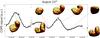 |
Fig. 1 ROSINA COPS neutral density measurements for August 23 2014 are shown in black for two cometary rotations together with associated illumination conditions on the nucleus. Color coded on the nucleus is the cosine of the solar zenith angle θ for different time instances as seen from the s/c. For cases with a large total illuminated area and visible surface area of the nucleus the COPS data peaks, which lead to the fundamental assumption of the correlation between insolation and gas production rate. Narrow shaped features and gaps in the data are not of cometary origin and discussed in Sect. 2.4. |
Hässig et al. (2015) show from mass spectrometric measurements with ROSINA that even at a heliocentric distance of 3.5 AU, H2O is the most abundant species for a large fraction of the time. Overall, the gas production of 67P is dominated by H2O, CO, and CO2. We assume H2O to be the most abundant species for most of the dataset, and we are aware that this assumption is not always true. For certain time periods Hässig et al. (2015) show CO2 to be more abundant than H2O. We compare our simulation results to ROSINA COPS measurements, which cannot distinguish between the different species in the coma, and the signal is a linear combination of all species. As a consequence we do not attempt to model multiple species in our simulations. The neutral number densities obtained by ROSINA are measurements along the spacecraft (s/c) trajectory, typically 10 to 100 km from the comet surface. Therefore the observed coma features cannot necessarily be directly linked to features on the surface itself. This is partially due to the large field of view of nearly 4π for the COPS sensor. Furthermore, the sublimation process on the cometary surface is not well understood at this point and even for low gas production rates there are only a few collisions per molecule on its way to the s/c. As a consequence, gas from a large fraction of the surface can potentially reach the s/c location, making a radial mapping of outgassing features to the sub-spacecraft point an oversimplification.
2. Model and data description
This section gives a description of the three numerical models and the corresponding boundary conditions used for this study.
We consider three different numerical models, varying largely in complexity, implemented physics and computational cost. The kinetic model AMPS (Adaptive Mesh Particle Simulator), is considered the most appropriate tool for set task because it has most relevant physical processes included, but also is the computationally most expensive model. In contrast, the illumination model, which has a slightly lower agreement with the measured data, is computationally very cheap but includes much less physics. All three models produce similar results and this increases our confidence in the individual numerical schemes and the choice of boundary conditions. All discussed models use the SHAP4 mesh of 67P, which is constructed from the high resolution pictures taken with the Rosetta OSIRIS camera (Jorda 2015) and is shown in Fig. 1. We downsample the mesh from originally more than 8 × 10⁵ facets by roughly a factor of 5 to a coarser mesh of 1.6 × 10⁵ facets. This helps to decrease the computational cost for the hydrodynamic and kinetic models described in Sects. 2.2 and 2.3, but still provides a fine enough resolution of the nucleus for the purposes of our simulations. Section 2.4 contains some details about the ROSINA COPS data and the processing thereof. All presented model calculations are driven by the solar illumination conditions. To fit the COPS observations we can adjust two parameters for the hydrodynamic and the kinetic model which determine the maximum and minimum flux of every surface element depending on the solar zenith angle. The values of these parameters Fmin and Fmax are given in Table 1 and equally apply to all surface elements. In Sects. 3.3 and 3.4 we examine two correction factors that are applied in a post processing manner to the model outputs to improve the correlation between the models and observations. All models consider only one species, namely H2O neutrals for the kinetic and hydrodynamic simulations. The illumination model is independent of the species as it does not model a gas coma itself.
Physical quantities included for all AMPS and BATS-R-US simulations.
Both the kinetic model AMPS and the hydrodynamic code BATS-R-US (Block Adaptive Tree Solar-wind Roe Upwind Scheme) are massively parallel codes developed at the University of Michigan and have been applied to multiple large scale simulations over recent years (Tenishev et al. 2013, 2008; Fougere et al. 2013; Powell et al. 1999). The major differences between the codes are the numerical schemes to solve for different physical quantities. BATS-R-US treats the neutral gas as a fluid and solves the hydrodynamical equations accounting for conservation of mass, momentum, and energy. The kinetic model AMPS is a direct simulation Monte Carlo (DSMC) code where a finite number of discrete particles is simulated to solve the Boltzmann equation. The advantage of the kinetic approach is the ability to correctly take the conditions of a rarefied coma into account where the mean free path is large and collisions between neutrals mostly happen near to the nucleus, whereas the outer part of the coma is mostly collisionless. Both codes use an adaptive mesh refinement (AMR; Keppens et al. 2003) approach, which allows the model resolution to be locally increased where necessary and as a consequence reduces the computational cost. In the case of simulating 67P the highest resolution is used close to the nucleus to capture the exceptional geometric features of the body and resolve the local mean free path of the gas close to the surface.
2.1. Illumination model
The first model is of a geometric nature, holding the basic idea of the gas production rate being a function of the insolation of each surface element on the nucleus. All surface elements have an identical response to the illumination conditions they are exposed to. Accurate positions and attitudes of the Rosetta spacecraft, 67P, and the Sun are therefore calculated from the SPICE library with a temporal resolution of 20 min, starting from 6th August 2014 and ranging until the end of the year 2014. For every surface element of the nucleus, Ai, visible by the s/c, the surface area Si, solar zenith angle θi, and the angle between the surface normal to the spacecraft φi are calculated. The illumination model calculates a measure, Rillu, for the local number density at the s/c as 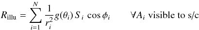 (1)where ri is the distance from the surface element to the s/c and g(θi) a function defined below. This assumes the individual production rates vary with the cosine of the solar zenith angle. Rillu corresponds to the total illuminated surface area on the nucleus, projected towards the spacecraft position by the cosφi factor. We note that the condition “visible to s/c” is not fulfilled by cosφi> 0 because the nucleus is not a convex object and parts of the surface can be blocked from view even with the surface normal pointing towards the s/c. We therefore numerically check for every Ai if there is a direct line of sight to the s/c and towards the Sun. The function g(θi) in Eq. (1) takes into account a floor limit for the production rate of surface elements being on the night side or in the shadow and is defined as following definition
 ![\begin{equation} g(\theta_i) = \max[a, \cos\theta_i] \end{equation}](/articles/aa/full_html/2015/11/aa26178-15/aa26178-15-eq29.png) (2)with a = 0.1, setting the floor value for the night side activity to 10% of the maximum. Finally, to compare Rillu, which has units of square meters, to the neutral number densities of COPS we multiply it by a constant. It is important to state that Rillu is a measure of the total illumination on the surface, which is not necessarily correlated to the local illumination conditions of the sub-spacecraft point (or the remote sensing instrument’s footprint) on the nucleus, as work by Lee et al. (2015) shows.
(2)with a = 0.1, setting the floor value for the night side activity to 10% of the maximum. Finally, to compare Rillu, which has units of square meters, to the neutral number densities of COPS we multiply it by a constant. It is important to state that Rillu is a measure of the total illumination on the surface, which is not necessarily correlated to the local illumination conditions of the sub-spacecraft point (or the remote sensing instrument’s footprint) on the nucleus, as work by Lee et al. (2015) shows.
2.2. Hydrodynamic model (BATS-R-US)
The hydrodynamic model is based on the BATS-R-US code (Powell et al. 1999; Tóth et al. 2012) that solves the Euler equations on a 3D block adaptive Cartesian grid. The molecular mass is M = 18 Da for the dominant H2O molecules, and the adiabatic index is γ = 4/3. We use a coordinate system that co-rotates with the comet. At a rotation rate of 12.4 h (Mottola et al. 2014), the inertial forces are negligible for gas calculations. The rotation axis is the z axis, while the x axis is at the zero longitude of the comet coordinate system. The computational domain extends to ± 640 km along all axes. The neutral gas flows out freely at the outer boundaries of the simulation domain, where the grid cell size is about 20 km.
The comet is kept at the origin of the comet fixed coordinate system, where the grid is refined with a resolution of 156 m and the grid cells inside the comet surface are excluded from the calculation. The inner boundary conditions are applied at the cell faces that separate the grid cells inside and outside of the comet, respectively. For each Cartesian cell face we find the facet of the shape model that is intersected by the line segment connecting the inside and outside cell centers. Next we obtain the surface normal n of the facet and calculate the cosine of the solar zenith angle cosθ = n·s, where s is the unit vector pointing towards the Sun. If cosθ> 0 and the facet is not in the shadow (i.e., the line pointing in direction s does not intersect any part of the surface), the particle flux and temperature are set as ![\begin{eqnarray} F &=& F_{\min} + (F_{\max} - F_{\min})\cos\theta \label{eq:F}\\ T &=& \max[T_{\min}, T_{\max} + \Delta T (1 - 1/\cos\theta)], \label{eq:T} \end{eqnarray}](/articles/aa/full_html/2015/11/aa26178-15/aa26178-15-eq40.png) where Fmin = 5 × 10¹⁷ m-2 s-2, Fmax = 7 × 10¹⁸ m-2 s-2, Tmin = 133 K, Tmax = 182.1 K and ΔT = 15.36 K. These functions are fits to the tabulated thermo-physical model by Davidsson et al. (2007). If cosθ< 0 or the facet is in the shade we set F = Fmin and T = Tmin according to Table 1. The night side production rate of 7% relative to the dayside, which is determined by Fmin, is taking contributions from CO and CO2 into account and in agreement with Davidsson et al. (2007). Considering the relative abundances by Hässig et al. (2015) this seems a valid choice for heliocentric distances of >2.6 AU. Temperatures used in this study are lower than the surface temperatures reported by Capaccioni et al. (2015) for measurements with the Rosetta-VIRTIS instrument. We assume the sublimation layer to be colder than the VIRTIS temperatures, which is consistent with their findings that the surface of 67P is almost free of ice and the significantly lower temperatures found by Gulkis et al. (2015) below the surface. We further assume that the sublimating gas does not thermally accommodate to the top surface temperature while diffusing outward. The temperature T and particle flux F describe a half-Maxwellian distribution escaping from the surface of the comet. This distribution is expected to thermalize within a small distance in the Knudsen layer.
where Fmin = 5 × 10¹⁷ m-2 s-2, Fmax = 7 × 10¹⁸ m-2 s-2, Tmin = 133 K, Tmax = 182.1 K and ΔT = 15.36 K. These functions are fits to the tabulated thermo-physical model by Davidsson et al. (2007). If cosθ< 0 or the facet is in the shade we set F = Fmin and T = Tmin according to Table 1. The night side production rate of 7% relative to the dayside, which is determined by Fmin, is taking contributions from CO and CO2 into account and in agreement with Davidsson et al. (2007). Considering the relative abundances by Hässig et al. (2015) this seems a valid choice for heliocentric distances of >2.6 AU. Temperatures used in this study are lower than the surface temperatures reported by Capaccioni et al. (2015) for measurements with the Rosetta-VIRTIS instrument. We assume the sublimation layer to be colder than the VIRTIS temperatures, which is consistent with their findings that the surface of 67P is almost free of ice and the significantly lower temperatures found by Gulkis et al. (2015) below the surface. We further assume that the sublimating gas does not thermally accommodate to the top surface temperature while diffusing outward. The temperature T and particle flux F describe a half-Maxwellian distribution escaping from the surface of the comet. This distribution is expected to thermalize within a small distance in the Knudsen layer.
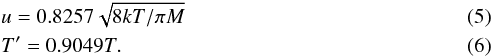
Following Huebner & Markiewicz (2000) and using the coefficients for frv = 3 in their Table 1, we set
 The density, velocity, and pressure of the hydrodynamic model at the cell face are then set as
 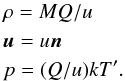 In the co-rotating frame the rotation of the comet corresponds to a rotation of the s vector pointing towards the Sun which is updated with 1 deg increments during the simulation. The solar latitude is kept fixed during each simulation. We therefore obtain 360 steady state solutions for a given solar latitude. The BATS-R-US code can simulate a full rotation in about 45 min on 720 cores.
2.3. Kinetic model (AMPS)
The kinetic modeling of the coma is performed with the Adaptive Mesh Particle Simulator (AMPS), which is a direct simulation Monte Carlo particle code that can solve the Boltzmann equation for a multi species environment. In this study we only present results for a single species, which is assumed to be H2O. Following the Monte Carlo approach, AMPS represents the gas flow by a large but finite number of simulation particles. The dynamics of those particles is governed by the physical laws describing the interactions of real atoms and molecules in a gas, including, for example, realistic collision cross sections between neutrals. All macroscopic parameters, such as bulk velocity, number density, or temperature of the gas are computed by sampling the microscopic properties (such as position and velocity) of a representative ensemble of particles. The DSMC approach is valid for all collisional regimes encountered in the cometary coma, from collision dominated near the nucleus surface to almost collision free after a few cometary radii. Except for the innermost part of the cometary coma, the collision frequency is insufficient to maintain equilibrium. Individual particles are injected into the simulation domain from the surface facets of the 3D shape model with the boundary conditions determined by Eqs. (3) and (4) the same way as for BATS-R-US. The velocities of the ejected particles follow the two distribution functions ![\begin{eqnarray} && f(v_{x}) \propto v_{x}\exp(-\beta^2v_{x}^2)\\[2mm] && f(v_y, v_z) \propto \exp(-\beta^2(v_y^2+v_z^2)), \end{eqnarray}](/articles/aa/full_html/2015/11/aa26178-15/aa26178-15-eq56.png) where the vx component is parallel to the local surface normal and vy and vz perpendicular to it and
where the vx component is parallel to the local surface normal and vy and vz perpendicular to it and  . AMPS has already been used for cometary applications, notably to describe the complex coma of Comet 103P/Hartley 2 by Fougere et al. (2013). The 3D extension of the cometary model was recently implemented and tested with spherical and irregular nucleus shapes by Fougere (2014).
Simulation details for AMPS and BATS-R-US.
2.4. Data treatment
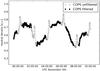 |
Fig. 2 White circles indicate unfiltered COPS signal in arbitrary units for 5th November. Six distinct peaks due to changes in the s/c attitude are identified and filtered out. The filtering is not based on a peak detection algorithm, but triggered by changes in s/c attitude solely. |
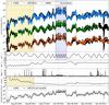 |
Fig. 3 Overview of the model results and comparison to COPS data. In this figure all model results do include correction factors for an increasing activity and latitudinal effects, described in Sects. 3.3 and 3.4. The top panel shows neutral density measurements as full black circles. For sake of visual clarity the COPS data is drawn in units of molecules/cm3 only for the comparison with BATS-R-US. Model results and data are scaled by 2 or 4 orders of magnitude, respectively, for comparison with AMPS and the Illumination model. All model results follow the large scale trends of the COPS measurements for the full dataset. The approximately 600 diurnal variations cannot be resolved in this image. The next 4 panels from the top show information on s/c attitude and position relative to 67P and the Sun, with LAT being the latitude of the s/c position radially projected onto the nucleus in degrees. The phase angle (PA) is defined as the angle Sun-67P-Rosetta, and also given in degrees. Finally ONA stands for off-nadir-angle, measured as the angle between the s/c z-axis and the vector pointing to the center of mass of the nucleus. The light yellow box marks a period where the COPS signal is mostly driven by the change in distance between Rosetta and 67P. For data in the light purple box the main driver for the large scale features are changes in latitude, while cometocentric distance (r), and phase angle remain relatively stable. The bottom panel shows COPS data and BATS-R-US data with smoothed out diurnal variations as described in Sect. 3.2. |
ROSINA COPS is an in situ instrument consisting of two separate sensors, a detailed description can be found in (Balsiger et al. 2007). The nude gauge (NG) measures the total ambient neutral number density at the s/c position. The ram gauge, which is normally pointing at the comet, measures the ram pressure of the outflowing gas of the neutral coma. All data presented in this study are from the NG sensor alone, making the comparison with the model outputs straightforward as the neutral density is a standard quantity produced. COPS cannot distinguish between different species in the coma, the signal is thus a linear combination of the abundances of the dominant species, which are H2O, CO and CO2Hässig et al. (2015) with H2O being the most abundant throughout the majority of the investigated time period. We therefore assume that the COPS signal mostly shows the same characteristics as H2O. In their recent work, Bockelée-Morvan et al. (2015) indeed find that water production rates are lower over nucleus areas with low illumination. Our boundary conditions are hence a reasonable choice for the description of neutral H2O. On the other hand they find CO2 to be much less affected by the illumination conditions as they report significant production rates thereof also on poorly illuminated areas. It is important to keep in mind that our model results are hence most reliable in cases with high H2O abundances. As reported by Schlaeppi et al. (2010) during the cruise phase of the Rosetta mission, the mass spectrometer and NG data are sensitive to attitude changes of the s/c. As a consequence, all COPS data where the s/c attitude is changing by more than 0.5 deg in between two measurements are rejected, so are data points where the total off-nadir angle (ONA) is larger than 20 deg. So even though COPS has a field of view of almost 4π steradian and is an in situ instrument it is sensitive to small changes in attitude of the Rosetta spacecraft. A typical effect of such maneuvers is shown in Fig. 2, which shows the COPS data with and without filtering by the attitude criteria described above. Such attitude correction maneuvers happen every few hours, making them a rather frequent disturbance in the dataset. More extensive maneuvers are usually caused by remote sensing instrument campaigns that have to fulfill very specific pointing requirements to perform, for example a limb scan for an extended time period. This filtering is especially critical for regions in the dataset where the COPS signal from the coma is low, say below 107 molecules per cubic cm, here a significant modification of the signal can be caused by this effect.
3. Model validation
In this section we compare our model outputs to ROSINA COPS measurements to examine the quality of agreement and draw conclusions about the outgassing properties of 67P. The top panel of Fig. 3 shows an overview comparison of all three model outputs with the full COPS dataset ranging from early August 2014 to 1st January 2015. Diurnal variations can not be resolved for this extensive time period in one plot, but instead can be seen in Fig. 4 that spans over a shorter time period. The following bottom 4 panels in Fig. 3 show data on the s/c attitude and position relative to the comet throughout the mission.
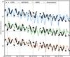 |
Fig. 4 Diurnal variations are reproduced by all models for the majority of the dataset. The format is the same as for Fig. 3 COPS and model data scaled by 1 or 2 orders of magnitude respectively for visual clarity. |
There are three main parameters one can see having an impact on the measurements:
- i)
distance r between the s/c and 67P: this is mostly important forthe first 6 weeks of data where Rosetta was still approaching thecomet. This period is indicated by a light yellow background inFig. 3 and is discussed in Sect. 3.1.From mid-September 2014 onwards, changes in distance occuron short time scales followed by longer periods with only minormodifications.
- ii)
Longitude and diurnal variations: due to the slow speed of Rosetta in the cometary frame of reference, longitude changes constantly with the rotation period of 67P. A clear modulation of the COPS signal with the same frequency can be identified throughout the whole dataset and a representative period is shown in Fig. 4. As later discussed in Sect. 3.2, this is strongly tied to the peculiar shape of 67P as it rotates with respect to the spacecraft position.
- iii)
Spacecraft latitude, measured as the radial projection of the s/c position in the body centric “Cheops” coordinate system rotating with the comet nucleus (Jorda 2015). Latitude changes occur during the whole dataset, the light purple box in Fig. 3 indicates a segment where latitude is the only parameter that is significantly changing over time as discussed in Sect. 3.3. Additional factors:
- iv)
Phase angle: for most of the time after 1st October Rosetta is in terminator orbits, at a phase angle of around 90 deg. There is no clear evidence for the influence of the phase angle on the measured signal. In the first 6 weeks of the data, the phase angle changes significantly, but so do the radial distance and the latitude. A systematic treatment of the effect resulting from changes in phase angle is not feasible with the current dataset.
- v)
Spacecraft attitude: as discussed in Sect. 2.4, pointing has a rather strong effect on the COPS signal. However, it does not contain any significant information on the coma structure. Therefore, data points with high off nadir pointing and during attitude changes are filtered out.
- vi)
The latitude of the Sun in the comet fixed frame changes by about 10 deg over the whole time period covered. AMPS and BATS-R-US simulations were carried out with the assumption of a fixed latitude of around 44 deg, which corresponds to the value in August. In addition, a second set of runs with the correct solar latitude for the month of December 2014 was performed for BATS-R-US. The changes observed from this latitude correction are noticeable, but not significant for the covered data range and hence not further included in this study.
- vii)
Thermal lag: We do not consider any thermal lag in our models. We assume a surface element on the nucleus instantaneously reaches the temperature defined by the model of Davidsson et al. (2007) as described above. This is clearly not a physical behavior, as surface patches currently in the shadow might have been fully illuminated shortly before. A more advanced nucleus model providing realistic temperature maps has to be considered for future studies. Furthermore we do not consider self illumination of surface patches from other parts of the nucleus. As Keller et al. (2015) show in their recent work, this can have a significant effect on the energy flux of surface elements for certain regions such as the neck.
3.1. Effects from radial distance
The most dominant parameter early on in the mission on the neutral gas number density is the distance of the s/c relative to the comet. This phase is indicated by the light yellow region in Fig. 3. The correlation between local number density as a function of radial distance is nicely reproduced by all the models. The illumination model takes the distance into account by an analytical 1 /r2 scaling law, which we find to be a reasonable fit. BATS-R-US and AMPS naturally produce 1 /r2 number density profiles because the gas is not accelerated for the most part of the outflow. This part can be considered clearly understood and no further improvements on the models are necessary in that regard.
3.2. Diurnal variations
As diurnal variations we define the peaks appearing in the COPS data at frequencies of the cometary rotation period of 12.4 h or 6.2 h respectively. Figure 4 shows how all models reproduce these features over an extended period of time. This is generally true for the whole dataset, except the first days of August where there is a significant phase shift between the peaks in the model results and the data over several cometary rotations. The shift is observed for data from 6th to 10th August 2014 where the simulated features lead the peaks in measured densities by 1 to 2 h. This effect is not understood at the moment and has only been observed for this earliest phase where the Rosetta s/c was farther away from 67P (120 km to 80 km) than during the rest of the year. Delay due to the finite outflow velocity of the gas can be neglected as with speeds of a few 100 ms–1 the time to reach 100 km is only a few minutes. Furthermore, the geometric illumination model is not able to reproduce all of those diurnal features. Except for the time period from 19 to 27 of September 2014, where the illumination model signature shows half the COPS signal frequency, when only every second peak is reproduced, these features are missed only sporadically. AMPS and BATS-R-US are able to match the data during this time period, using the same illumination data as boundary conditions.
Amplitudes of the diurnal variations are not reproduced as well from the models as are the frequencies thereof. The BATS-R-US solution tends to underestimate the local minima between two peaks, as can be seen during the last few oscillations in Fig. 4. For the kinetic AMPS solution, the temporal resolution is much lower, hence the peaks and minima are not always sampled. This can result in an underestimation of the total amplitude of the diurnal variations.
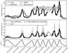 |
Fig. 5 Top panel: smoothed COPS and all model data. Clearly the models are not able to reproduce the large scale variations observed. Between October 13 and 26 the model average is more or less a horizontal line with little variation over time. Bottom panel: smoothed and original COPS data together with smoothed illumination model data with applied latitude correction. The fit between the large scale features and the model is significantly increased. The same applies for averaged AMPS and BATS-R-US data which are not shown in this plot. |
3.3. Heterogeneity effects
Figure 5 shows data from terminator orbits at distances from 20 km to 10 km away from the nucleus. This marks the immediate pre-lander phase of the mission and is the only time in 2014 where the s/c is very close to the nucleus. During this phase, the only significant changes are in the projected cometary latitude, while the distance to the comet and the phase angle are relatively constant. The model and COPS data presented in the top panel of Fig. 5 are filtered using the Savitzky-Golay method (Savitzky & Golay 1964) to smooth out diurnal effects. To see the effect of the Savitzky-Golay filtering, see the bottom panel of Fig. 5 where the unfiltered data is still shown as a gray line. What is left is the effect of the latitude changes on the signal (radial distance and phase angle are constant). As seen in the top panel of Fig. 5 this is not reproduced by any of the models as all of them assume homogeneous outgassing properties over the whole surface. This suggests a large scale heterogeneity in the coma of 67P with enhanced H2O abundance towards northern latitudes. Coma heterogeneity for 67P has previously been reported by Hässig et al. (2015).
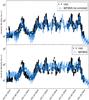 |
Fig. 6 The effect of the latitude correction shown for BATS-R-US model results. The top panel shows the increased agreement with the COPS observations after applying the correction. In this figure none of the signals is filtered or smoothed in any way, hence the diurnal variations are clearly noticeable. |
The introduction of a correction factor correlated with latitude improves the match between data and model for both the smoothed and original cases as shown in Figs. 6 and 5. The correction applied is a post process multiplication with the sine of the latitude that has a floor value of 0.3. ![\begin{eqnarray*} C_{\rm LAT}=2\max[\sin\text{LAT},\:0.3]. \end{eqnarray*}](/articles/aa/full_html/2015/11/aa26178-15/aa26178-15-eq68.png) This correction has no physical rationale but attempts to describe a large scale heterogeneity in the coma with enhanced number densities towards northern latitudes. The floor value is introduced by the observation of the COPS signal from 4 to 9 of October 2014 (see Fig. 5 bottom panel). During this time period the s/c latitude is constantly changing between 25 deg and −50 deg. At the same time the COPS signal is very stable. The same applies for 11 to 13 of October. Although in the top panel of Fig. 5 it looks like on 10 October the models do reproduce some latitudinal effect, this is actually caused by a simultaneous decrease in radial distance, which causes the peak in the simulation data. The same applies for the increase in signal on 14 October and the decrease on 30 October. Finding the physical cause of this latitude dependence is beyond the scope of this paper and will require measurements of individual gas species in the coma and temperature measurements on the nucleus. As such it will be addressed in future work to get a more self-consistent description of these latitudinal effects. However, such a large scale heterogeneity is observed by various instruments on board Rosetta. Feldman et al. (2015) report such findings for measurements taken with the UV spectrograph ALICE. They measure the strongest emissions for late 2014 at northern sub-spacecraft latitudes. Wurz et al. (2015) report highest abundances of neutral H2O for northern (positive) latitudes in the coma of 67P. Those measurements were performed with the ROSINA-DFMS mass spectrometer during several days along a bound orbit at ≈10 km distance from the nucleus.
This correction has no physical rationale but attempts to describe a large scale heterogeneity in the coma with enhanced number densities towards northern latitudes. The floor value is introduced by the observation of the COPS signal from 4 to 9 of October 2014 (see Fig. 5 bottom panel). During this time period the s/c latitude is constantly changing between 25 deg and −50 deg. At the same time the COPS signal is very stable. The same applies for 11 to 13 of October. Although in the top panel of Fig. 5 it looks like on 10 October the models do reproduce some latitudinal effect, this is actually caused by a simultaneous decrease in radial distance, which causes the peak in the simulation data. The same applies for the increase in signal on 14 October and the decrease on 30 October. Finding the physical cause of this latitude dependence is beyond the scope of this paper and will require measurements of individual gas species in the coma and temperature measurements on the nucleus. As such it will be addressed in future work to get a more self-consistent description of these latitudinal effects. However, such a large scale heterogeneity is observed by various instruments on board Rosetta. Feldman et al. (2015) report such findings for measurements taken with the UV spectrograph ALICE. They measure the strongest emissions for late 2014 at northern sub-spacecraft latitudes. Wurz et al. (2015) report highest abundances of neutral H2O for northern (positive) latitudes in the coma of 67P. Those measurements were performed with the ROSINA-DFMS mass spectrometer during several days along a bound orbit at ≈10 km distance from the nucleus.
3.4. Increase in production rate
Heliocentric distance of 67P varies from 3.6 AU in early August to 2.6 AU at the end of 2014. Despite the decrease in heliocentric distance we find that a constant production rate from August to 1 November fits the COPS data best. Bockelée-Morvan et al. (2015) similarly report no significant increase in the total H2O production rate for heliocentric distances from 2.9 to 2.5 AU as measured with the Rosetta VIRTIS instrument. We can calculate the total production rate of 67P by integrating the fluxes of all the model facets over the total surface area. This leads to total production rates of Qtotal = 8.7 × 1025 s-1−1.1 × 1026 s-1, depending on the illumination conditions. This is slightly higher than the observed total production rate of 4 × 1025 s-1 for H2O in August 2014 as reported by Gulkis et al. (2015). We note that we estimate the total production rate of 67P which only gives an upper limit for the H2O production rate. For data after 1 November we get the best fit with our models for a production rate that is increased by a factor of 2. From the model comparison the increase in activity happened within a few days between end of October and early November, after being constant for several months. The activity increase was fitted by analysis of the absolute error and correlation coefficient between model and observations described in the next section. As seen in panel B) of Fig. 7, a fixed production rate systematically underestimates the observations for data points taken after 1 November. We note that this apparent increase in activity is not understood and coincides with the s/c leaving the terminator orbits. This might hence be an effect from a change in the geometry of the observation, or changes in activity are less prominent around the terminator and the actually more continuous increase was therefore only observed after leaving the terminator orbits.
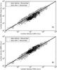 |
Fig. 7 Two scatter plots showing the correlation between AMPS results and COPS measurements. For panel A) the production rate Q is assumed constant over the whole time period of 2014. Clearly all simulation results after 1 November then underestimate the observations. Panel B) shows the AMPS results if we take into account an increase in the production rate of a factor of 2, leading to better agreement. |
3.5. Model quantification
In this section we quantify the quality of the model solutions by computing correlation coefficients between data and model results. The procedure is explained individually for every model below. Thereby we can examine the effects of the correction factors introduced for the latitudinal effects and the increase in activity described in Sects. 3.3 and 3.4. The improvement on the three models by applying these corrections is summarized in Table 3. This approach is computationally much cheaper than repeated runs for all models, which typically need a few 10 k of CPU hours to produce results. Although ad hoc, some valuable information can be gained from this analysis, which will help improve the next generation of our physics driven models AMPS and BATS-R-US.
Summary of the correction term effects on the model data correlation.
3.5.1. Comparison with the illumination model
The model calculates Rillu with a time resolution of 20 min between 6 August 2014 and 1 January 2015. For every Rillu we look for a COPS measurement that is as close as possible in time. If the time difference between the model point and the COPS measurement is less than 10 min, both data points are taken into account for the correlation calculation. If no such pair can be found (e.g., COPS was not operating for a certain period, or the measurements were filtered out because of pointing criteria), the data point from the model is ignored.
3.5.2. Comparison with AMPS
Every AMPS run corresponds to a certain longitude of the Sun in the cometary reference frame (latitude is assumed constant). Now for every COPS measurement we check if there is an AMPS run with longitude within 10 deg of the values for the measurement. As an example, one AMPS run was done for longitude = 60 deg. This means all COPS data where the projected Sun longitude was between 50 and 70 deg are compared to this AMPS run. The six model runs hence cover a total of 6 × 20 = 120 deg, which means that roughly 1/3 of all COPS measurements are compared to AMPS.
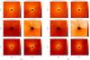 |
Fig. 8 AMPS and BATS-R-US comparison for number density, velocity and pressure. Panel a) corresponds to the z = 0 plane in the comet centered coordiante system and b) to the plane with y = 0. The simulated Sun position in all figures is on the positive y-axis at x = 0 km. On the left hand side of each panel we show results from AMPS and on the right hand side from BATS-R-US. For BATS-R-US, there are structures in the number density and pressure profiles which are not seen for AMPS. Gas velocities produced by AMPS are in better agreement with the velocity of 0.68 km s-1 reported by Gulkis et al. (2015). Both methods produce asymmetric number density and velocity profiles with higher abundances and velocities on the hemisphere pointed towards the Sun. |
3.5.3. Comparison with BATS-R-US
Comparison with COPS data is done with the following procedure. For each point along Rosetta’s trajectory we calculate the solar longitude and the position of the spacecraft in the cometary frame from SPICE kernels. Then we take the one out of 360 model solutions with the most similar solar longitude and interpolate the number density from the discrete simulation grid to the position of Rosetta. The change in the solar latitude can also be taken into account by doing multiple simulations with different latitude values.
3.5.4. AMPS and BATS-R-US comparison
In Fig. 8 we can look at a direct comparison between the kinetic and hydrodynamic solutions in terms of number density, velocity, and pressure. The panels on the left hand side in both figures are results from AMPS, on the right hand side BATS-R-US. There is a good agreement in terms of absolute values for number density and pressure between the two models in both the y = 0 and z = 0 planes. Differences show up in the global structure of the coma, AMPS produces a smoother profile with gradients pointing about radially away from the nucleus, whereas we can see clear structures in the number density and pressure profiles for the BATS-R-US results. In case of the kinetic solution produced by AMPS, there are almost no collisions between the outflowing neutrals for a large fraction of the coma, with the exception of the inner most part close to the nucleus. Once in the collisionless region, the neutrals hence flow out on approximately straight lines, but with random directions, which smooths out any structure in the coma the farther away from the nucleus we look. On the other hand, the fully collisional fluid assumption made in BATS-R-US allows for interaction between intersecting flow patterns, which then produce an approximately radial outflow and more pronounced longitudinal and latitudinal variations depicted in 8. For the gas velocity we observe a significant difference between the two models, with AMPS producing lower speed gas flows than BATS-R-US. This occurs even though both models assume the same surface temperature and velocity distribution at the nucleus. BATS-R-US produces these higher velocities on both the day and night side of the coma. The measured expansion velocity, reported by Gulkis et al. (2015) of 0.68 km s-1 are somewhat lower than the BATS-R-US velocities computed for the day side and show better agreement with AMPS.
4. Conclusion
We successfully validated our numerical models by implementing solar insolation as the main driver of activity on the cometary surface. We are able to reproduce the ROSINA COPS measurements and their variations over several months and a wide range of spacecraft locations and nucleus illumination conditions. To reproduce the diurnal variations observed by COPS, models need to take the realistic 3D shape model of 67P into account. Both physics driven models AMPS and BATS-R-US do reproduce more of the diurnal variations than the geometric illumination model and do show better agreement with the observations. This indicates that the physical processes during the outflow are non-negligible even at large heliocentric distances, and backtracking of coma features to the nucleus is non-trivial. Our study suggests that, despite the assumption of a fluid regime, hydrodynamic simulations such as BATS-R-US are able to describe the neutral coma properties of 67P reasonably well. This is remarkable as our simulations extend out to 3.5 AU and 67P is considered a very weakly outgassing comet. Finding a procedure for a correct mapping of coma features to the nucleus is beyond the scope of this paper, but has to be addressed in the future. We see evidence for large scale heterogeneity of neutral gas in the coma, with increasing number densities towards northern latitudes. Again, drawing conclusions about the cause of this heterogeneity is currently not possible by analysis of in situ data. Hence, this has only been addressed by introducing a correction factor to the model results that takes a latitudinal dependence into account. In future studies a self-consistent approach has to be developed to accurately characterize this correlation directly in the models. In summary we find that COPS measurements can be reproduced by models considering a mostly homogeneous activity and a night side activity of 7% to 10% relative to the dayside. This was achieved by the assumption that all surface elements of 67P increase activity if illuminated. This does not exclude the presence of a large number of smaller scale features on the nucleus that contribute to the overall activity. We however predict these features to be distributed over a large fraction of the nucleus, which then cannot be distinguished by COPS measurements from the strictly homogeneous case. Measurements with the OSIRIS camera system indeed show that all illuminated areas on the northern hemisphere show activity between December 2014 and January 2015 (Keller et al. 2015). The model agreement can further be improved by the introduction of a latitudinal dependence and an increase in the total production rate by a factor of two after 1 November. A constant production rate of Qtotal ≈ 1 × 1026 s-1 is found to best reproduce the observed data up to 1 November 2014.
Acknowledgments
The authors would like to thank the following institutions and agencies, which supported this work: Work at the University of Michigan was funded by NASA under contract JPL-1266313. Work at UoB was funded by the State of Bern, the Swiss National Science Foundation and by the European Space Agency PRODEX Program. Work at Southwest Research institute was supported by subcontract #1496541 from the Jet Propulsion Laboratory. Work at BIRA-IASB was supported by the Belgian Science Policy Office via PRODEX/ROSINA PEA 90020. This work was supported by CNES grants at IRAP, LATMOS, LPC2E, UTINAM, CRPG. ROSINA would not give such outstanding results without the work of the many engineers, technicians, and scientists involved in the mission, in the Rosetta spacecraft, and in the ROSINA instrument team over the last 20 yr whose contributions are gratefully acknowledged. Rosetta is an ESA mission with contributions from its member states and NASA. We acknowledge herewith the work of the whole ESA Rosetta team. All ROSINA data will be released to the PSA archive of ESA and to the PDS archive of NASA.
References
- A’Hearn, M. F., Belton, M. J. S., Delamere, W. A., et al. 2011, Science, 332, 1396 [NASA ADS] [CrossRef] [Google Scholar]
- Balsiger, H., Altwegg, K., Bochsler, P., et al. 2007, Space Sci. Rev., 128, 745 [NASA ADS] [CrossRef] [Google Scholar]
- Bockelée-Morvan, D., Debout, V., Erard, S., et al. 2015, A&A, 583, A6 [NASA ADS] [CrossRef] [EDP Sciences] [Google Scholar]
- Capaccioni, F., Coradini, A., Filacchione, G., et al. 2015, Science, 347 [Google Scholar]
- Combi, M. R., Tenishev, V. M., Rubin, M., Fougere, N., & Gombosi, T. 2012, ApJ, 749, 13 [Google Scholar]
- Davidsson, B. J., Gutiérrez, P. J., & Rickman, H. 2007, Icarus, 191, 547 [NASA ADS] [CrossRef] [Google Scholar]
- Farnham, T., Bodewits, D., Li, J.-Y., et al. 2013, Icarus, 222, 540 [NASA ADS] [CrossRef] [Google Scholar]
- Feldman, P., A’Hearn, M., Bertraux, J.-L., et al. 2015, A&A, 583, A8 [NASA ADS] [CrossRef] [EDP Sciences] [Google Scholar]
- Fougere, N. 2014, Ph.D. Thesis, University of Michigan, Department of Atmospheric Oceanic and Space Science [Google Scholar]
- Fougere, N., Combi, M., Rubin, M., & Tenishev, V. 2013, Icarus, 225, 688 [NASA ADS] [CrossRef] [Google Scholar]
- Gulkis, S., Allen, M., von Allmen, P., et al. 2015, Science, 347 [Google Scholar]
- Hässig, M., Altwegg, K., Balsiger, H., et al. 2015, Science, 347 [Google Scholar]
- Huebner, W., & Markiewicz, W. 2000, Icarus, 148, 594 [NASA ADS] [CrossRef] [Google Scholar]
- Jorda, L., & Gaskell, R. H. 2015, Shape models of 67P/Churyumov-Gerasimenko, RO-C-OSINAC/OSIWAC-5-67P-SHAPE-V1.0, NASA Planetary Data System and ESA Planetary Science Archive [Google Scholar]
- Keller, H. U., Mottola, S., Davidsson, B., et al. 2015, A&A, 583, A34 [NASA ADS] [CrossRef] [EDP Sciences] [Google Scholar]
- Keppens, R., Nool, M., Tóth, G., & Goedbloed, J. 2003, Comput. Phys. Commun., 153, 317 [NASA ADS] [CrossRef] [Google Scholar]
- Knight, M. M., & Schleicher, D. G. 2013, Icarus, 222, 691 [NASA ADS] [CrossRef] [Google Scholar]
- Lee, S., von Allmen, P., Allen, M., et al. 2015, A&A, 583, A5 [NASA ADS] [CrossRef] [EDP Sciences] [Google Scholar]
- Powell, K. G., Roe, P. L., Linde, T. J., Gombosi, T. I., & De Zeeuw, D. L. 1999, J. Comput. Phys., 154, 284 [NASA ADS] [CrossRef] [Google Scholar]
- Mottola, S., Lowry, S., Snodgrass, C., et al. 2014, A&A, 569, L2 [NASA ADS] [CrossRef] [EDP Sciences] [Google Scholar]
- Savitzky, A., & Golay, M. J. E. 1964, Anal. Chem., 36, 1627 [NASA ADS] [CrossRef] [Google Scholar]
- Schlaeppi, B., Altwegg, K., Balsiger, H., et al. 2010, J. Geophys. Res., 115 [Google Scholar]
- Tenishev, V. M., Combi, M., & Davidsson, B. 2008, ApJ, 685, 659 [NASA ADS] [CrossRef] [Google Scholar]
- Tenishev, V., Rubin, M., Tucker, O. J., Combi, M. R., & Sarantos, M. 2013, Icarus, 226, 1538 [NASA ADS] [CrossRef] [Google Scholar]
- Tóth, G., van der Holst, B., Sokolov, I. V., et al. 2012, J. Comput. Phys., 231, 870 [Google Scholar]
- Wurz, P., Rubin, M., Altwegg, K., et al. 2015, A&A, 583, A22 [NASA ADS] [CrossRef] [EDP Sciences] [Google Scholar]
All Tables
All Figures
|
Fig. 1 ROSINA COPS neutral density measurements for August 23 2014 are shown in black for two cometary rotations together with associated illumination conditions on the nucleus. Color coded on the nucleus is the cosine of the solar zenith angle θ for different time instances as seen from the s/c. For cases with a large total illuminated area and visible surface area of the nucleus the COPS data peaks, which lead to the fundamental assumption of the correlation between insolation and gas production rate. Narrow shaped features and gaps in the data are not of cometary origin and discussed in Sect. 2.4. |
| In the text | |
|
Fig. 2 White circles indicate unfiltered COPS signal in arbitrary units for 5th November. Six distinct peaks due to changes in the s/c attitude are identified and filtered out. The filtering is not based on a peak detection algorithm, but triggered by changes in s/c attitude solely. |
| In the text | |
|
Fig. 3 Overview of the model results and comparison to COPS data. In this figure all model results do include correction factors for an increasing activity and latitudinal effects, described in Sects. 3.3 and 3.4. The top panel shows neutral density measurements as full black circles. For sake of visual clarity the COPS data is drawn in units of molecules/cm3 only for the comparison with BATS-R-US. Model results and data are scaled by 2 or 4 orders of magnitude, respectively, for comparison with AMPS and the Illumination model. All model results follow the large scale trends of the COPS measurements for the full dataset. The approximately 600 diurnal variations cannot be resolved in this image. The next 4 panels from the top show information on s/c attitude and position relative to 67P and the Sun, with LAT being the latitude of the s/c position radially projected onto the nucleus in degrees. The phase angle (PA) is defined as the angle Sun-67P-Rosetta, and also given in degrees. Finally ONA stands for off-nadir-angle, measured as the angle between the s/c z-axis and the vector pointing to the center of mass of the nucleus. The light yellow box marks a period where the COPS signal is mostly driven by the change in distance between Rosetta and 67P. For data in the light purple box the main driver for the large scale features are changes in latitude, while cometocentric distance (r), and phase angle remain relatively stable. The bottom panel shows COPS data and BATS-R-US data with smoothed out diurnal variations as described in Sect. 3.2. |
| In the text | |
|
Fig. 4 Diurnal variations are reproduced by all models for the majority of the dataset. The format is the same as for Fig. 3 COPS and model data scaled by 1 or 2 orders of magnitude respectively for visual clarity. |
| In the text | |
|
Fig. 5 Top panel: smoothed COPS and all model data. Clearly the models are not able to reproduce the large scale variations observed. Between October 13 and 26 the model average is more or less a horizontal line with little variation over time. Bottom panel: smoothed and original COPS data together with smoothed illumination model data with applied latitude correction. The fit between the large scale features and the model is significantly increased. The same applies for averaged AMPS and BATS-R-US data which are not shown in this plot. |
| In the text | |
|
Fig. 6 The effect of the latitude correction shown for BATS-R-US model results. The top panel shows the increased agreement with the COPS observations after applying the correction. In this figure none of the signals is filtered or smoothed in any way, hence the diurnal variations are clearly noticeable. |
| In the text | |
|
Fig. 7 Two scatter plots showing the correlation between AMPS results and COPS measurements. For panel A) the production rate Q is assumed constant over the whole time period of 2014. Clearly all simulation results after 1 November then underestimate the observations. Panel B) shows the AMPS results if we take into account an increase in the production rate of a factor of 2, leading to better agreement. |
| In the text | |
|
Fig. 8 AMPS and BATS-R-US comparison for number density, velocity and pressure. Panel a) corresponds to the z = 0 plane in the comet centered coordiante system and b) to the plane with y = 0. The simulated Sun position in all figures is on the positive y-axis at x = 0 km. On the left hand side of each panel we show results from AMPS and on the right hand side from BATS-R-US. For BATS-R-US, there are structures in the number density and pressure profiles which are not seen for AMPS. Gas velocities produced by AMPS are in better agreement with the velocity of 0.68 km s-1 reported by Gulkis et al. (2015). Both methods produce asymmetric number density and velocity profiles with higher abundances and velocities on the hemisphere pointed towards the Sun. |
| In the text | |
Current usage metrics show cumulative count of Article Views (full-text article views including HTML views, PDF and ePub downloads, according to the available data) and Abstracts Views on Vision4Press platform.
Data correspond to usage on the plateform after 2015. The current usage metrics is available 48-96 hours after online publication and is updated daily on week days.
Initial download of the metrics may take a while.