| Issue |
A&A
Volume 583, November 2015
Rosetta mission results pre-perihelion
|
|
|---|---|---|
| Article Number | A5 | |
| Number of page(s) | 10 | |
| Section | Planets and planetary systems | |
| DOI | https://doi.org/10.1051/0004-6361/201526155 | |
| Published online | 30 October 2015 | |
Spatial and diurnal variation of water outgassing on comet 67P/Churyumov-Gerasimenko observed from Rosetta/MIRO in August 2014
1 Jet Propulsion Laboratory, California Institute of Technology, 4800 Oak Grove Dr., Pasadena, CA 91109, USA
e-mail: This email address is being protected from spambots. You need JavaScript enabled to view it.
2 LERMA, Observatoire de Paris, PSL Research University, CNRS, UMR 8112, UPMC, 75014 Paris, France
3 LESIA-Observatoire de Paris, CNRS, UPMC, Université Paris-Diderot, 5 place Jules Janssen, 92195 Meudon, France
4 Max-Planck-Institut für Sonnensystemforschung, Justus-von-Liebig-Weg 3, 37077 Göttingen, Germany
5 National Central University, 300 Jhongli, Taiwan
6 University of Massachusetts, 619 Lederle Graduate Research Tower, Amherst, MA, USA
7 Planetary Science Institute, 1700 East Fort Lowell, Suite 106, Tucson, AZ 85719, USA
8 Laboratoire d’Astrophysique de Marseille, BP 8, 13376 Marseille Cedex 12, France
9 Institute for Geophysics and extraterrestrial Physics, 38106 TU Braunschweig, Germany
Received: 22 March 2015
Accepted: 21 June 2015
Abstract
Aims. We present the spatial and diurnal variation of water outgassing on comet 67P/Churyumov-Gerasimenko using the H216O rotational transition line at 556.936 GHz observed from Rosetta/MIRO in August 2014.
Methods. The water line was analyzed with a non-LTE radiative transfer model and an optimal estimation method to retrieve the H216O outgassing intensity, expansion velocity, and gas kinetic temperature. On August 7−9, 2014 and August 18−19, 2014, MIRO performed long steady nadir-pointing observations of the nucleus while it was rotating around its spin axis. The ground track of the MIRO beam during the observation was mostly on the northern hemisphere of comet 67P, covering its three distinct parts: the so-called head, body, and neck areas.
Results. The MIRO spectral observation data show that the water-outgassing intensity varies by a factor of 30, from 0.1 × 1025 molecules s-1 sr-1 to 3.0 × 1025 molecules s-1 sr-1, the terminal gas expansion velocity varies by 0.17 km s-1 from 0.61 km s-1 to 0.78 km s-1, and the terminal gas temperature varies by 27 K from 47 K to 74 K. The retrieved coma parameters are co-registered with local environment variables such as the subsurface temperatures, measured in the MIRO continuum bands, the local solar time, illumination condition, and beam location on nucleus. The spatial variation of the outgassing activity is very noticeable, and the largest outgassing activity in August 2014 occurs near the neck region of the nucleus. The outgassing activity in the neck region is also found to be correlated with the local solar hour, which is related to the local illumination condition.
Key words: comets: individual: 67P/Churyumov-Gerasimenko / solid state: volatile / radiation mechanisms: thermal
Distinguished visiting scientists at the Jet Propulsion Laboratory.
Retired.
© ESO, 2015
1. Introduction
Since May 2014, the Microwave Instrument on the Rosetta Orbiter (MIRO) has observed comet 67P/Churyumov-Gerasimenko (67P) in two frequency bands at 190 GHz and 562 GHz. A spectrometer is connected to the 562 GHz receiver and was designed to observe the molecular lines of H O, H
O, H O, H
O, H O, CO, NH3, and CH3OH volatiles emitted from the cometary nucleus. The scientific goals of the spectral observations are to assess the abundances and isotopic ratios of cometary volatiles and to understand the spatial distribution and temporal evolution of the activity. The first spectral line emission from comet 67P detected by MIRO was the HO 110−101 ortho-rotational transition line at 556.936 GHz. It was first observed on June 6−7, 2014 at a heliocentric distance of 3.9 AU and at a MIRO-to-comet distance of 360 000 km (Gulkis et al. 2015). Images from OSIRIS onboard Rosetta also show the activity of comet 67P in June and as early as March 2014 (Tubiana et al. 2015). Since the first detection, MIRO has observed this line on a regular basis in the nadir-pointing and the coma-scanning modes, while the Rosetta spacecraft approached the comet from >100 000 km to <100 km, making it possible to track the spatial distribution and temporal evolution of the water-outgassing activity. In this paper, we present MIRO HO spectral line observations and line analysis retrieval results and discuss the implications for the temporal evolution of the water-outgassing activity and its spatial distribution. The rotational line of HO line was studied in Gulkis et al. (2015).
2. Observations
On August 7−9, 2014 and August 18−19, 2014, MIRO performed long steady nadir-pointing observations of the nucleus while it was rotating around its spin axis. The ground track of the MIRO submillimeter beam was mostly located in the northern hemisphere of comet 67P, covering its so-called head, body, and neck regions. The comet’s heliocentric distance ranged from 3.60 AU to 3.52 AU, and the spacecraft distance to the comet center ranged from 78 km to 107 km. Since the MIRO beam angular extension is 7.5 arcmin in terms of its full width at half maximum (FWHM), the MIRO beam diameter at half maximum on the nucleus ranged from 170 m to 230 m. This set of observational data covers a sizable area of the nucleus in the northern hemisphere and provides good coverage of the local solar time. The long stable pointing enables the acquisition of spectra with a reasonably long integration time from a localized beam on the nucleus, leading to a high signal-to-noise ratio. Therefore, this dataset is useful for studying the spatial and diurnal variations of the water-outgassing activity. Our study uses an integration time of 10 min, which provides a good signal-to-noise ratio for the HO line. It should be noted that this dataset presents finer temporal and therefore spatial sampling than the study of the HO line in Gulkis et al. (2015), where an integration time of 30 min was used to achieve a sufficiently high signal-to-noise ratio.
Figure 1a shows the ground track of the MIRO beam during the nadir observations. The circles show the locations of the MIRO sub-millimeter beam center averaged over 10 min. The color indicates the MIRO submillimeter continuum receiver antenna temperature, which is related to the subsurface temperature of the nucleus at a depth of about 1−2 cm (Gulkis et al. 2015; Schloerb et al. 2015). To calculate the latitude and longitude of the MIRO beam location, we used the OSIRIS SHAP2 model (Sierks et al. 2015). The gray contour plots the elevation from the nucleus center of mass. Figure 1b is a 3D projection of the nucleus of 67P with the MIRO beam locations illustrated on the 3D shape. The mean illumination of the local location in August 2014 is highlighted in gray.
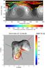 |
Fig. 1 Ground-track of MIRO submillimeter beam during the two steady nadir-pointing observations in August 7−9 and August 18−19 in the latitude-longitude map (top panel) and the 3D nucleus shape (bottom panel). Each circle shows the mean location for a period of 10 min. The color of the circle gives the MIRO submillimeter continuum receiver antenna temperature, which is related to the subsurface temperature of the nucleus at the time of observation (Gulkis et al. 2015). The gray contour plots the elevation from the nucleus center of mass in the top panel and the mean illumination in the bottom panel. |
During the nadir observations, MIRO simultaneously detected both the HO rotational ground-state transition line at 556.936 GHz using the Chirp Transform Spectrometer and the nucleus thermal emission with the continuum channels of the submillimeter heterodyne receiver. Figure 2 shows the time series of the line and continuum emissions. The time series of the line was obtained by integrating the absolute value of the line area in such a way that the emission and absorption components in the line shape are added together instead of being subtracted. In the nadir-pointing observation geometry most of the observed lines contained only an absorption signal and the continuum signal was high; the brightness temperature was higher than 100 K.
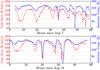 |
Fig. 2 Time series of the submillimeter receiver antenna temperature and H |
For short periods of time, part or most of the MIRO beam was pointing off the nucleus due to the irregular shape of the nucleus, even though the Rosetta/MIRO pointing relative to the comet center of mass was mostly fixed. When a portion of the beam was pointing off the nucleus, the continuum emission became very low and the spectral line became an emission line showing a positive value for positive Doppler velocities. For example, a portion of the MIRO beam was pointing off the nucleus at around 36 h and 48 h elapsed since midnight on August 7, and 20 h and 32 h elapsed since midnight on August 18.
Figure 3 shows the three types of line shapes we obtained during our observations. Type 1 is an absorption line for negative Doppler velocities, where the gas moving toward MIRO absorbs the thermal emission from the nucleus. This type of line shape is observed when the MIRO beam is fully located on the nucleus. Type 2 consists of an absorption component for negative Doppler velocities and an emission component for positive Doppler velocities. This type of line shape is observed when the MIRO beam is only partially located on the nucleus. The absorption component of the line shape originates from the absorption of the thermal emission from the nucleus by the gas in front of the nucleus, while the emission component originates from the emission by the gas located behind the nucleus. Type 3 is an emission line for both negative and positive Doppler velocities. This type of line shape is obtained when the MIRO beam pointing is fully off the nucleus. Both the gas in front and the gas behind the nucleus produce emission lines at their corresponding Doppler velocities. The present study solely focuses on the first type of line shape, where the MIRO beam is fully located on the nucleus. The transition from emission to absorption line shape is also clearly seen for HO data in Biver et al. (2015).
 |
Fig. 3 Three types of line shapes measured during nadir-pointing MIRO observations on August 7−9 and 18−19. The first type is obtained when the MIRO beam was fully on nucleus, the second type when the beam was partially on nucleus, and the third type when the beam was fully off nucleus. |
3. Models and data analyses
The MIRO spectral data were analyzed using a specified coma model and a radiative transfer calculation. The coma model provides the spatial distribution of the water gas density, velocity, and temperature. We used a parameterized coma model and assumed that the coma properties vary along the line of sight in the way they would vary in a spherically symmetric coma. This approximation is equivalent to assuming that all the measured column abundance of water along the line of sight enters the line of sight at locations near the footprint of the beam, neglecting contributions from regions of the nucleus far away from the location of the MIRO beam footprint. In the specific case of observations in the neck region, for example, we neglect contributions from the head and body regions. This assumption appears as very limiting and an unrealistic description of the 3D coma structure for an irregular nucleus shape like that of 67P, which the OSIRIS camera, for example, has shown to feature a strong inhomogeneity of the outgassing sources (e.g., jets), leading to inhomogeneity in the coma (Sierks et al. 2015). However, we believe our approach to be a reasonable first-order approximation to analyze the data considered in this study. We point out specific deficiencies of the model as we encounter them in the course of the data analysis.
The total water gas density profile along the line of sight was parameterized with the Haser model as follows: 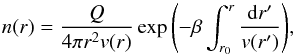 (1)where n(r) is the profile of the gas density in molecules m-3, Q/4π the outgassing intensity in molecules s-1 sr-1, v(r) the radial profile of the expansion velocity in m s-1, β the photodissociation rate in s-1, and r the distance from the comet center in m. The value used for β was determined by using the value of 1.36 × 10⁻⁵ (s-1) at a heliocentric distance of 1.0 AU, as given by Biver et al. (2009), and by scaling with a
  factor for a specific heliocentric distance RH. The photodissociation rate varies with the solar activity, and the rate for the quiet-Sun activity is 1.26 × 10⁻⁵ (s-1) (Crovisier 1989). The photodisocciation rate is not a critical parameter for this study because all the observations probed gas near the nucleus: <100 km from the nucleus.
We assumed an ortho-to-para water ratio of 3 to relate the total water density profile to the ortho water density profile, which is needed to calculate the population of the rotational levels of the ortho water in the radiative transfer model described below. While the ratio of 3 is taken from the statistical equilibrium value, some previous measurements of comets found a lower ortho-to-para ratio. For example, a ratio of 2.6 ± 0.3 is reported for comet C/2001 Q4 (Kawakita et al. 2006) and a ratio of 2.1 ± 0.1 for comet 1P/Halley (Mumma et al. 1988). The lower ratio leads to a higher ratio of the total water density to the ortho water density, which in turn results in a higher total water-outgassing rate for a given ortho water density profile. When the ortho-to-para ratio of 2.1 is used instead of 3.0, the increase of the total water-outgassing rate is ~ 10%. This is within the uncertainty of our retrieval analysis due to measured spectrum noise, model assumption dependence, and calibration error.
The profile of the gas velocity was parameterized with the following two-parameter hyperbolic tangent function: 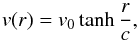 (2)where v0 is the terminal or asymptotic velocity at large distance, and c is the parameter that controls how fast the velocity initially monotonically increases with distance. This parameterization was inspired by a direct simulation Monte Carlo (DSMC) calculation for the one-dimensional coma structure (Davidsson et al. 2010), where the resulting velocity profile shows a rapid monotonic increase initially followed by a slow asymptotic approach to the terminal velocity (the maximum value). The shape of this variation is well captured with this two-parameter hyperbolic tangent function.
The profile of the gas temperature was parameterized with the following two-parameter function:  (3)where T0 is a constant and was fixed to 150 K, a is the scaling factor for the 1 /r dependence of the temperature profile, b is the scaling factor for the terminal or asymptotic value of the gas temperature as the distance increases, and r0 is a constant set to 2 km. This parameterization was also inspired by a DSMC simulation of the coma structure (Lee et al. 2011; Davidsson et al. 2010). The resulting temperature profile shows a rapid monotonic decrease initially followed by a slow asymptotic approach to the terminal temperature (the minimum value). The shape of this variation can be well reproduced by the two-parameter function in Eq. (3).
The coma model is fully described with these three profiles, which contain a total of five free parameters: Q in the density profile, v0 and c in the velocity profile, and a and b in the temperature profile. The model used in Gulkis et al. (2015) for the analysis of the HO emission line assumed a constant expansion velocity and a fixed gas temperature profile, where the profile is parameterized with Eq. (3) similar to the present study, but the parameters a and b were fixed for all the lines studied.
After defining the coma model, we calculated the non-local thermal equilibrium (non-LTE) population of the rotational levels for the ortho HO molecules as they move away from the nucleus. For the radiative transfer we assumed a spherical coma. The rate equation for the ortho HO rotational population levels includes radiative coupling, collisions with neutral water molecules, collisions with electrons, and infrared radiative pumping. The rate equation is described in detail in Lee et al. (2011). The average radiation intensity that is needed in the rate equation can be accurately calculated with a direct ray transfer sampling approach such as the accelerated Monte Carlo method (Hogerheijde & van der Tak 2000). However, this calculation is computationally very demanding because of the large sampling needed to reach convergence. We instead used a local approximation, called the escape probability method, which is described in Litvak & Kuiper (1982) and Bockelée-Morvan (1987). Zakharov et al. (2007) showed that differences in the level populations between the two methods do not exceed 20%, that the line areas differ by less than 7%, and that the line shapes agree excellently well. The gas production rates for 67P in August 2014 are lower than those for which this excellent agreement between the two methods was obtained. We used the escape probability method in this study nonetheless and assumed that the two methods agree sufficiently well to validate our conclusions.
The synthetic water line spectra were calculated based on published parameters for the MIRO instrument (Gulkis et al. 2007). The MIRO beam shape was approximated with a Gaussian function with a full width at half maximum of 7.5 arcmin. The synthetic power received by the MIRO radiometer was converted to antenna temperature to compare with the calibrated line spectra of the MIRO measurement. The details of the line spectrum calculation are described in Lee et al. (2011).
4. Retrieving the coma parameter
We retrieved the coma profiles by fitting the synthetic to the observed line spectra using optimal estimation (Rodgers 2000). The coma parameters were retrieved by iterating the following process until a convergence criterion is met:
-
1.
A coma profile was initially defined with five freeparameters (Q, a, b, v0, c).
-
2.
For a given coma profile, the rotational level population of the ortho water near the H
O transition line at 557 GHz was calculated using the non-LTE molecular excitation model. -
3.
Using the resulting level population and the assumed coma profile, the line shape for the H
O transition was computed with the radiative transfer model. -
4.
The synthetic and measured line shapes were compared in terms of a cost function that is described below in more detail.
-
5.
A new coma profile was calculated by using the Jacobian matrix of the cost function with respect to the retrieval parameters. The convergence scheme follows the direction that leads to the largest decrease in the cost function during each iteration.
-
6.
We returned to step 1 and repeated until the process converged (e.g., the cost function reached a minimum threshold).
In step 4, the cost function involves both the difference between the line spectrum values and the difference between the retrieval parameters at this iteration and a priori retrieval parameters. The second term in the cost function takes into account any prior knowledge or constraint on the coma profile. It is usually determined by the retrieval result for a spectrum observed nearby in time and space. The cost function also takes into account the uncertainty of each component: uncertainty on the line spectrum measurement and uncertainty on the a priori retrieval parameters. The measurement uncertainty can be estimated from the noise in the measured line spectrum, which is affected by a combination of thermal noise and gain fluctuation present in the receiver. The uncertainty on the a priori retrieval parameters is estimated from the uncertainty in the previous retrieval result, which defines the a priori vector. We find that the measurement uncertainty is typically about 1 K for a spectral resolution of 100 kHz and an integration time of 10 min. The uncertainty on the a priori retrieval parameters was set to be relatively large to avoid biasing the search in the retrieval parameter space. It was typically set to about 100% relative uncertainty for each parameter. In this way, the selected a priori parameters provide guidance in the retrieval search space but do not strongly restrict the search.
We applied this retrieval method to the absorption-only lines measured during the nadir-pointing observations. We first integrated the spectral lines over 10 min and resampled the spectral lines with a 100 kHz resolution to reduce the noise level. After time integration and spectral resolution adjustment, the noise level was around 1 K.
Figure 4 shows the outgassing intensity (Q/ 4π) as retrieved from each spectral line in the observation dataset. The spectral line area divided by the submillimeter antenna temperature, as measured in the MIRO continuum channel, is also plotted for comparison. We obtain excellent qualitative agreement between the two time series, as expected for optically thin lines since the relative line area is directly proportional to the column density in this case. We note that the variation of the relative line area has a smaller amplitude than that of the water-outgassing variation. An examination of the line shapes shows that saturation effects can explain this behavior. The time series of the retrieved water-outgassing intensity shows stronger short-term fluctuations than that of the line area, which might point to instabilities in the retrieval algorithm. Since we retrieve not only the outgassing intensity, but also four other coma parameters simultaneously, and the five parameters are connected with a nonlinear system of equations (i.e. the non-LTE radiative transfer equation and coma model), it is difficult to guarantee that the global optimum is always found. In addition, our coma model assumes that the density, temperature, and velocity profiles are fully determined by the outgassing near the location of the MIRO footprint. The degree to which the real coma structure matches the parameterized model will determine the relevance of the retrieved solution to the real coma parameters and will affect the correlation between the retrieved outgassing rate and the integrated line area. The good overall agreement between the two time series leads us to conclude that, on average, the retrieval algorithm is reliable.
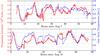 |
Fig. 4 Time series of the retrieved water-outgassing intensity (red solid line) compared with the H |
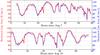 |
Fig. 5 Time series of the retrieved line area (red solid line) compared with the measured line area (blue dashed line). Overall, the agreement is good. The small deviations in the line area for some cases (e.g. 24 h since 0 h on August 7 and 8 h since 0 h on August 18) can be traced back to a complex observed line shape, which cannot be reproduced with the parameterized coma model used in this study. |
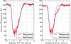 |
Fig. 6 Comparison of the measured and retrieved spectra for two cases. The left panel shows a case where the measured spectral line shape is well reproduced by the retrieved spectral line. The right panel shows a case where the retrieved spectral line shape does not agree well with the observed line. The observed line shows an extended absorption area for positive Doppler velocities, while the retrieved line lacks this feature. The shoulder in the absorption line is due to molecules moving away from the observer (MIRO) and cannot be explained within the approximations of the coma model used in this study. |
To assess the quality of the model parameter fit, the retrieved and measured line areas are compared in Fig. 5. In most cases, we obtain good agreement. When the retrieved and measured areas deviate significantly, we note that the retrieved outgassing intensity also shows a strong fluctuation in Fig. 4. We found that the measured spectral lines in these cases have a more complex line shape than in the cases where the retrieval is successful, as shown in Fig. 6. The complex line shape includes an extended absorption region for positive Doppler velocities, which indicates that the line is broadened by molecules moving toward the nucleus.
In our coma model, the gas along the line of sight to the nucleus cannot have a mean velocity pointing toward the nucleus. Therefore, any broadening of the line into the range of positive Doppler velocities comes from thermal broadening, which can indeed produce the large absorption shoulder shown in Fig. 6 (right panel) for functional profiles of the expansion velocity and temperatures different from those described in Eqs. (2) and (3). In particular, we find that the amplitude and extension of the shoulder for positive Doppler velocities is highly dependent on the velocity profile parameter c and the temperature profile parameter a. These two parameters control how fast the temperature and velocity profiles change with respect to the distance to the nucleus. Since we constrained the velocity and temperature variations to the parameterized profiles given in Eqs. (2) and (3), it is expected that some details of the line shape cannot be reproduced. To reproduce line shapes like the one in the right panel of Fig. 6 more accurately, one needs to involve a three-dimensional (3D) coma structure, where the mean gas velocity in the probed column density receives contributions from regions on the nucleus other than those near the location of the MIRO footprint. Preliminary 3D calculations of the gas density and velocity distributions around a non-spherical nucleus do explain the presence of an extended shoulder at positive Doppler velocities as shown in Fig. 6, but it is beyond the scope of this publication to consider a fully 3D coma structure. Therefore we limit our study to the retrieved dataset that reproduces the line shape and area of the measured line as shown in the left panel of Fig. 6.
We next examined the correlations among the retrieved coma parameters. Since these parameters are physically coupled through the processes of gas dynamics in the coma, some level of correlation is expected between the retrieved values. The DSMC calculations by Davidsson et al. show that the outgassing intensity and the terminal expansion velocity are positively correlated, while the outgassing intensity and the terminal gas temperature are negatively correlated (Davidsson et al. 2010). The positive correlation of the outgassing intensity with the terminal expansion velocity is due to the higher kinetic energy imparted to the molecules at high outgassing intensity. The negative correlation between the outgassing intensity and the terminal temperature can be seen as a result of the isentropic expansion where the temperature and expansion velocity are inversely correlated. At large distances, this correlation would break down due to photochemical heating processes, for example, which lead to a simultaneous increase of the temperature and expansion velocity (Combi et al. 1997). When we retrieve the five coma parameters, no explicit relationship among them is prescribed. Therefore, it is important to check whether the retrieved parameters preserve the physical consistency governed by the gas dynamics. Figure 7 shows the distribution of the water-outgassing intensity versus the expansion velocity and that of the water-outgassing intensity versus the gas temperature. The distributions confirm that the retrieved parameters exhibit the physically expected correlations and that our retrieval method generates physically consistent coma parameters.
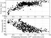 |
Fig. 7 Distributions of the retrieved gas parameters. The top panel shows a scatter plot of the outgassing intensity and terminal expansion velocity. The bottom panel shows a scatter plot of the outgassing intensity and terminal gas temperature. The outgassing intensity is overall positively correlated with the terminal expansion velocity, while the outgassing intensity is overall negatively correlated with the terminal gas temperature. These correlations of the retrieved parameters are consistent with the results of gas dynamics simulations, even though no explicit relationship among the parameters was prescribed in the retrieval process. |
The uncertainty on the retrieved parameters was estimated by performing a sensitivity analysis on the line shape with respect to variations in the retrieved parameters. We find that the outgassing intensity affects the overall line area and width. A 20% variation of the outgassing intensity leads to an about 1 K change in the line spectra, which is the noise level observed in the measured target spectrum for a 10-minute integration time and at 100 kHz resolution. The uncertainty on the outgassing intensity is therefore taken to be about 20%.
The temperature profile parameter a affects the line shape on the positive Doppler velocity side of the spectra. We find that a 20% variation of parameter a leads to a change of 1 K in the line shape on the positive velocity side (corresponding to the noise level). The temperature profile parameter b strongly affects the minimum temperature of the line shape. We found that the noise level at the minimum temperature of the line shape is higher than the overall line shape noise level. We used 3 K as the uncertainty on the minimum temperature. A 5% variation of the parameter b leads to a change in the minimum temperature of 3 K, which corresponds to the measurement uncertainty.
The velocity profile parameter v0 determines the velocity location at the minimum-temperature line point and is very well constrained by our measured line spectrum. We find that a 10 m s-1 variation of v0 leads to a shift in the line center of 10 m s-1, which is easily detectable in the line spectrum. The frequency calibration error of the MIRO measured spectrum is about 25 m s-1, which approximately represents the width of one channel in the MIRO spectrometer. This means that the retrieval error on the velocity v0 is smaller than the calibration error. The velocity profile parameter c affects the line shape on the positive Doppler velocity side, similarly to the temperature profile parameter a. We find that a 2 km variation of this parameter causes a 1 K change in the line shape on the positive Doppler velocity side. The uncertainty on c is therefore taken to be 2 km. Table 1 summarizes the uncertainty on the five retrieved model parameters.
Retrieval uncertainty for the five model parameters for a 10-minute integration time of the MIRO spectrum and a 100 kHz resolution.
We note that the uncertainty on the retrieved parameters is strictly limited to the uncertainty for a given assumed coma profile structure. A change in the assumptions of the model for the coma profile can lead to a larger uncertainty in a physically comparable parameter such as the local outgassing intensity, the terminal temperature, and the terminal velocity.
5. Spatial variation
We now examine the origins of the strong variation in the outgassing intensity during our nadir-pointing observation. We first considered the spatial variation in terms of the location of the MIRO footprint on the nucleus. Figure 8 displays the retrieved outgassing intensity at the location of the MIRO beam on a cylindrical map of the nucleus. The distribution of the outgassing intensity reveals a strong spatial variation as well as a strong variation within a given location or vicinity. The outgassing activity can be affected by many local environmental factors. We list a few of them here: Obviously, the presence and amount of water ice will directly affect the local outgassing activity. The structure of the ice layer and the surrounding layers, such as the porosity of the top layer, will affect the permeability to the gas flow and in turn also the outgassing intensity. The local illumination conditions affect the surface temperature and the local temperature profile with depth, which determines the ice sublimation rate.
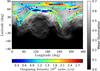 |
Fig. 8 Retrieved outgassing intensity at the location of the MIRO beam on the nucleus of 67P with a background image of the mean illumination in August 2014. |
The background image in Fig. 8 gives the mean diurnal illumination for the geometric configuration of the nucleus on August 15, 2014. Overall, most of the MIRO beam footprints in this study are located in well-illuminated parts of the nucleus. The mean diurnal illumination is calculated by taking the average of the projection of the Sun direction onto the local normal at each plate in the digital shape model. The average was taken over one spin period of the nucleus, and the time step for the time integration was 10 min. For each plate and each time, local shadowing effects were taken into account by determining all the intersections with the nucleus of a ray starting at the plate and pointing to the Sun. If an intersection was found between the plate and the Sun, the illumination was set to zero. The cylindrical map was calculated by finding the plates that intersect the local ray for a given latitude-longitude pair. In some regions of the nucleus, more than one plate was found due to the non-convexity of its shape. The mean illumination for the plate that is closest to the Sun was then taken for the map value at this latitude-longitude pair.
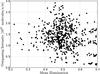 |
Fig. 9 Distribution of the outgassing intensity with respect to the mean illumination at the MIRO beam location on the nucleus. No obvious correlations or relationship are observed. |
The most active regions are notably located near the latitude of 80° North and longitudes in the 180°−240° range. The most active region does not coincide with the region with the highest mean illumination. There are many other regions with a mean illumination higher than or similar to the one in the most active region. Interestingly, the most illuminated area on the body shows the least outgassing activity. In addition, there are strong outgassing variations in areas with similar mean illumination. These observations indicate that the mean illumination is not the main factor driving the spatial variation of the activity level. Figure 9 further demonstrates that the correlation between the mean illumination and outgassing is weak. Since the mean illumination is the average over one spin period, we also checked the effect of the local illumination condition at the time of observation on the outgassing intensity. The incidence angle, which is the angle between the Sun direction and the local normal at the plate of the MIRO beam location, was calculated and plotted with the outgassing intensity. Figure 10 shows no strong correlation between the local incidence angle and the local outgassing intensity.
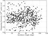 |
Fig. 10 Distribution of the outgassing intensity with respect to the incidence angle of the MIRO beam on the nucleus location. They do not exhibit any obvious correlations or relationships. |
Another potential source of the spatial variation is the temperature at the depth where the water ice resides. We checked whether the outgassing activity was correlated with the local subsurface temperature by using the MIRO submillimeter antenna temperature, which is related to the susurface temperature of the nucleus at depths of about 1−2 cm (Gulkis et al. 2015; Schloerb et al. 2015). Figure 11 shows the distribution of the local outgassing intensity with respect to the MIRO submillimeter antenna temperature. The peak value of the outgassing intensity for a given subsurface temperature shows a positive trend. However, the variation of the outgassing intensity for a given subsurface temperature is too strong to conclude that the outgassing intensity is directly correlated with the subsurface temperature.
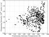 |
Fig. 11 Distribution of the outgassing intensity with respect to the MIRO submillimeter antenna temperature at the MIRO beam location on the nucleus. No obvious correlations or relationship is observed. |
If the sublimating ice is distributed uniformly over the nucleus and the structure of the ice and the surrounding layers is homogeneous, the outgassing activity is expected to be well correlated with the mean illumination at the corresponding location on the nucleus and the temperature at the depth where the ice resides. We find that the outgassing activity is not very well correlated with the local mean illumination or the local subsurface temperature. This is consistent with a heterogeneous distribution of the water ice and dust configuration on the nucleus, which could partly explain the spatial variation of the outgassing activity.
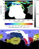 |
Fig. 12 Top panel: retrieved outgassing intensity at the location of the MIRO beam on the nucleus of 67P with the background image of the three distinctive parts of the nucleus shape: body (white), head (gray), and neck (black). Bottom panel: nineteen regions on the nucleus of 67P defined in Thomas et al. (2015). For some of the regions, acronyms are used for readability: at for Aten, Hh for Hathor, A for Apis, Sq for Serqet, N for Nut, and Hat for Hatmehit. |
We divided the nucleus of 67P into three distinctive areas called the head, body, and neck regions. Figure 12 illustrates the retrieved outgassing intensity with the head (white), body (gray), and neck (black) as the background color. The neck, body, and head regions on the nucleus were determined from the local Gauss curvature at each plate. The Gauss curvature is negative when the local topography is hyperboloid-like, positive on domes and pits, and zero for a flat surface. The Gauss curvature for each vertex on the surface was computed as described in Meyer et al. (2003) and an average was taken over the nearest-neighbor vertices to reduce the fast variations due to local topography. The neck is identified as the region on the surface of the nucleus where the local average of the Gauss curvature is negative. The body and head regions have positive curvature and were identified separately by crosschecking the regions on an orthogonal plane projection of the nucleus. Thomas et al. (2015) have defined nineteen regions on the nucleus of 67P based on surface morphology, structure, and topography. The bottom panel of Fig. 12 shows the regions on the latitude-longitude map. Most of the MIRO beam locations are in Hapi, Seth, and Ash. Hapi is the neck and is covered with smooth dusty-looking materials. Seth is in the body and shows brittle materials with active pits. Ash is the main dust-covered smooth region of the body.
Most of the MIRO measurements in this study are located in the neck region Hapi with some fraction in the head regions such as Seth and Ash and the body regions such as Ma’at and Hathor. We observed that the most active regions are in the neck, while some moderate activity regions are in the head. The body contains the least active regions. Several locations are sampled multiple times, and it is evident that there is a strong variation of the outgassing intensity even at the same location, revealing a temporal variation of the activity.
6. Diurnal variation
We observe a large spatial variation of the outgassing intensity, but even at the same location on the nucleus, there is still a strong variation in the outgassing intensity derived from our data, indicating a significant temporal variation. To what extent can the retrieved outgassing variation be ascribed either to a spatial variation or to a temporal variation of the activity? In an attempt to decouple the two variation sources, we collected the measurements from a limited small area, which is located at latitudes north of 80°N. This area covers a radius of 140 m at most because it is primarily located in the neck area near the north pole of the spin-axis. The area size is comparable with the MIRO beam size of about 100 m in radius during these observations. This area was sampled many times by the MIRO beam at various local times of the day.
Figure 13 shows the local retrieved water-outgassing intensity as a function of the local time of the day. The local time of the day was calculated using the hour angle between the effective longitude of the shape plate at the MIRO beam footprint and the subsolar longitude. The hour angle was scaled to be in the range of 0 to 24 h. The effective longitude was determined by the direction of the normal to the plate at the MIRO beam center averaged over the integration time of 10 min. The diurnal variation of the outgassing activity is clearly visible in the figure. The outgassing activity increases quickly after 14 h, reaches its maximum around 19 h, and then starts to decrease. The diurnal variation is about a factor of 2.2 from around 1025 molecules s-1 sr-1 in the morning to about 2.2 × 1025 molecules s-1 sr-1 at the peak.
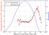 |
Fig. 13 Local water-outgassing intensity with respect to the effective local solar time, retrieved for locations on the nucleus at latitudes higher than 80°N. The effective local solar time is determined by calculating the angle between the direction of the local normal direction at the location of the MIRO center beam and the Sun direction. |
To understand this temporal variation, we calculated the illumination history of the region as shown in Fig. 13. This region enjoys a very long daylight time, which is approximately 21 h out of 24 h, using the local time of the day convention. This represents about 88% of the comet day. The only night time in this region is from 21 h to 24 h and is due to shadowing by the body. Interestingly, the onset time of the outgassing activity does not follow the illumination curve, but the offset time of the outgassing activity (19 h), where the activity starts to sharply decrease, is close to the sunset time of the region (21 h).
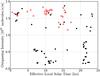 |
Fig. 14 Distribution of the outgassing intensity with respect to the effective local solar time for the measurement from the body of the nucleus with the latitude lower than 60°N. The data are divided into two groups with respect to the emission angle of the measurement. The red open circle group represents the data with an emission angle smaller than 40°. The black filled circle group represents the data with an emission angle larger than 40°. The emission angle is the angle between the direction of the MIRO line of sight and the direction normal to the plate where the MIRO beam intercepts the shape. The larger the emission angle, the weaker the effect on the measurement by the local outgassing activity at the MIRO beam location. |
We also examined the diurnal variation of another part of the nucleus: a region on the body with latitudes below 60° N. The bound on the latitude was imposed to minimize the effect of outgassing from the nearby neck region on the observation and retrieved outgassing rate. If all the measurements at this location are taken into consideration, the distribution is too noisy to show any pattern in the diurnal variation. We furthermore filtered the data with the emission angle since a large emission angle might cause the measurement to become more strongly affected by other sources than the source at the MIRO beam location. Figure 14 shows the diurnal variation of the outgassing rate in the body region with two subsets in the data: one with emission angles smaller than 40° (red circles) and the other with emission angles larger than 40° (black circles). The dataset with small emission angles shows an outgassing activity that remains relatively unchanged with the local time of the day covered in the data. An interesting trend is also that the gas emission rate appears to be higher for small emission angles. No clear diurnal variation of the outgassing intensity can hence be identified from the data selected in this study for latitudes lower than 60° N.
7. Discussion
Spectral observations of 67P were obtained by the MIRO instrument at 556.936 GHz for the HO rotational transition line. On August 7−9, 2014 and August 18−19, 2014, MIRO performed long steady nadir-pointing observations on the nucleus while the nucleus was rotating around its spin axis. The spectral observations were analyzed with a parameterized one-dimensional coma radial profile and a non-LTE radiative transfer model for the HO rotational transition line. The analysis of the MIRO spectral data shows that the water-outgassing rate varies by a factor of 30, from 0.1 × 1025 molecules s-1 sr-1 to 3.0 × 1025 molecules s-1 sr-1, the terminal gas expansion velocities vary by 0.17 km s-1 from 0.61 km s-1 to 0.78 km s-1, and the terminal gas temperatures vary by 27 K from 47 K to 74 K. These results are consistent with the results reported in Gulkis et al. (2015) for the HO line in the same time period. When the range of the outgassing intensity found in the present study is converted to a column density, it ranges from 0.07 × 10¹⁵ to 2.1 × 10¹⁵ molecules/cm2. Gulkis et al. (2015) reported that the column density ranges from 0.1 × 10¹⁵ to 2.0 × 10¹⁵ molecules/cm2, which excellently agrees with the range we found here. In addition, the temporal variation of the outgassing rate also agrees well. For example, the local maximum at 5 h on August 7 and the local minimum at 9 h on August 7 are found to be the same by us and Gulkis et al. (2015).
If the sublimating water ice were distributed uniformly over the nucleus, a simple coma model would lead to the expectation that the outgassing activity strongly correlates with the local mean illumination and the temperature at the depths where the ice resides. We find that the outgassing activity is not strongly correlated with the local mean illumination or the local subsurface temperature. Preliminary analysis of the contribution to the column density from other regions of the nucleus than locations near the MIRO footprint indicates that the variation of the outgassing is not solely driven by illumination. This suggests a heterogeneous distribution of sublimating ice and the dust environment on the nucleus. The most active region coincides with the neck area of the nucleus, suggesting a larger deposit of ices in the neck than in other parts of the nucleus. The VIRTIS spectrometer and the OSIRIS science camera on Rosetta have observed similar trends (Sierks et al. 2015; Capaccioni et al. 2015; Bockelée-Morvan et al. 2015). In addition, MIRO brightness temperatures in the neck region are consistent with sublimation of ice in the neck region, as the measured temperatures are lower than thermal model predictions of a pure dust layer with thermal inertia of 10−30 JK-1 m-2 s−1/2 (Schloerb et al. 2015). The same thermal model describes the measured temperatures in the other parts of the nucleus very well (Schloerb et al. 2015).
We found that part of the variation of the outgassing activity is determined by the diurnal cycle, depending on the effective local solar time of the day defined by the local normal to the shape relative to the subsolar longitude. The diurnal curve of the outgassing in the neck region, near the north pole (the positive spin axis direction), exhibits a variation of the outgassing rate by about a factor of 2. The diurnal variation partly follows the local illumination history of the region in the sense that the outgassing activity starts to rapidly decrease after the local sunset time. This indicates that the local outgassing activity is partly controlled by the diurnal cycle of the solar illumination. It also indicates that the sublimating ice is located within the diurnal thermal layer, which is expected to be within a depth of 1−2 cm (Gulkis et al. 2015). The diurnal variation in the body region was also investigated, but we found it to be too weak in this observation dataset.
The diurnal variation (about a factor of 2) in the neck region accounts for a small fraction of the global variation of the outgassing activity (about a factor of 30). This indicates that the spatial variation is significantly stronger than the diurnal variation. However, it is important to note that the diurnal variation in the north pole region does not necessarily explain the diurnal variation in all the other regions. More detailed diurnal and spatial sampling of the MIRO spectral observations is needed to fully determine the degree of the variability in terms of its source and to understand the mechanism of the diurnal variation and the source of the regional variation. Better fitting of the line shape and a better understanding of the correlation between illumination and outgassing activity can probably also be achieved with a model that takes into account the global contribution to the local column density from regions of the nucleus other than the location of the MIRO footprint.
Acknowledgments
The authors acknowledge support from their institutions and funding sources. A part of the research was carried out at the Jet Propulsion Laboratory, California Institute of Technology, under a contract with the National Aeronautics and Space Administration. A part of the research was carried out at the Max-Planck-Institut für Sonnensystemforschung with financial support from [DLR and MPG]. Parts of the research were carried out by LESIA and LERMA, Observatoire de Paris, with financial support from CNES and CNRS/INSU. A part of the research was carried out at the National Central University with funding from grant NSC 101-2111-M-008-016. A part of the research was carried out at the University of Massachusetts, Amherst, USA. We acknowledge personnel at ESA’s European Space Operations Center (ESOC) in Darmstadt, Germany and at ESA and NASA/JPL tracking stations for their professional work in communication with and directing the Rosetta spacecraft, thereby making this mission possible. We acknowledge the excellent support provided by the Rosetta teams at the European Space Operations Center (ESOC) in Germany, and the European Space Astronomy Center (ESAC) in Spain. The authors thank Holger Sierks and the OSIRIS team for permission to use the SHAP2 shape model for analysis purposes. We thank Nicolas Thomas and his group at the University of Bern, Switzerland for providing the map of the nineteen regions on the nucleus of 67P defined in Thomas et al. (2015).
References
- Biver, N., Bockelée-Morvan, D., Colom, P., et al. 2009, A&A, 501, 359 [NASA ADS] [CrossRef] [EDP Sciences] [Google Scholar]
- Biver, N., Hofstadter, M., Gulkis, S., et al. 2015, A&A, 583, A3 [NASA ADS] [CrossRef] [EDP Sciences] [Google Scholar]
- Bockelée-Morvan, D. 1987, A&A, 181, 169 [NASA ADS] [Google Scholar]
- Bockelée-Morvan, D., Debout, V., Erard, S., et al. 2015, A&A, 583, A6 [NASA ADS] [CrossRef] [EDP Sciences] [Google Scholar]
- Capaccioni, F., Coradini, A., Filacchione, G., et al. 2015, Science, 347, 0628 [NASA ADS] [CrossRef] [Google Scholar]
- Combi, M. R., Kabin, K., DeZeeuw, D. L., el al. 1997, Earth Moon and Planets, 79, 275 [Google Scholar]
- Crovisier, J. 1989, A&A, 213, 459 [NASA ADS] [Google Scholar]
- Davidsson, B. J. R., Gulkis, S., Alexander, C., et al. 2010, Icarus, 210, 455 [NASA ADS] [CrossRef] [Google Scholar]
- Gulkis, S., Frerking, M., Crovisier, J., et al. 2007, Space Sci. Rev., 128, 561 [NASA ADS] [CrossRef] [Google Scholar]
- Gulkis, S., Allen, M., von Allmen, P., et al. 2015, Science, 347, 0709 [Google Scholar]
- Hogerheijde, M. R., & van der Tak, F. F. S. 2000, A&A, 362, 697 [NASA ADS] [Google Scholar]
- Kawakita, H., Russo, N. D., Furusho, R., et al. 2006, ApJ, 643, 1337 [NASA ADS] [CrossRef] [Google Scholar]
- Lee, S., von Allmen, P., Kamp, L., et al. 2011, Icarus, 215, 721 [NASA ADS] [CrossRef] [Google Scholar]
- Litvak, M. M., & Rodriguez Kuiper, E. N. 1982, ApJ, 253, 622 [NASA ADS] [CrossRef] [Google Scholar]
- Meyer, M., Desbrun, M., Schroder, P., et al. 2003, in Visualization and Mathematics III, eds. H.-Ch. Hege, & K. Polthier (Berlin: Springer), 35 [Google Scholar]
- Mumma, M. J., Blass, W. E., Weaver, H. A., et al. 1998, in The Formation and Evolution of Planetary Systems, eds. H. A. Weaver, F. Paresce, & L. Danly (Baltimore: STScI), 157 [Google Scholar]
- Rodgers, C. D. 2000, Inverse Methods for Atmospheric Sounding: theory and practice (World Scientific Publishing) [Google Scholar]
- Schloerb, F. P., Keihm, S., von Allmen, P., et al. 2015, A&A, 583, A29 [NASA ADS] [CrossRef] [EDP Sciences] [Google Scholar]
- Sierks, H., Barbieri, C., Lamy, Ph. L., et al. 2015, Science, 347, aaa1044 [Google Scholar]
- Thomas, N., Sierks, H., Barbieri, C., et al. 2015, Science, 347, aaa0440 [Google Scholar]
- Tubiana, C., Snodgrass, C., Bertini, I., et al. 2015, A&A, 573, A62 [NASA ADS] [CrossRef] [EDP Sciences] [Google Scholar]
- Zakharov, V., Bockelée-Morvan, D., Biver, N., et al. 2007, A&A, 473, 303 [NASA ADS] [CrossRef] [EDP Sciences] [Google Scholar]
All Tables
Retrieval uncertainty for the five model parameters for a 10-minute integration time of the MIRO spectrum and a 100 kHz resolution.
All Figures
|
Fig. 1 Ground-track of MIRO submillimeter beam during the two steady nadir-pointing observations in August 7−9 and August 18−19 in the latitude-longitude map (top panel) and the 3D nucleus shape (bottom panel). Each circle shows the mean location for a period of 10 min. The color of the circle gives the MIRO submillimeter continuum receiver antenna temperature, which is related to the subsurface temperature of the nucleus at the time of observation (Gulkis et al. 2015). The gray contour plots the elevation from the nucleus center of mass in the top panel and the mean illumination in the bottom panel. |
| In the text | |
|
Fig. 2 Time series of the submillimeter receiver antenna temperature and H |
| In the text | |
|
Fig. 3 Three types of line shapes measured during nadir-pointing MIRO observations on August 7−9 and 18−19. The first type is obtained when the MIRO beam was fully on nucleus, the second type when the beam was partially on nucleus, and the third type when the beam was fully off nucleus. |
| In the text | |
|
Fig. 4 Time series of the retrieved water-outgassing intensity (red solid line) compared with the H |
| In the text | |
|
Fig. 5 Time series of the retrieved line area (red solid line) compared with the measured line area (blue dashed line). Overall, the agreement is good. The small deviations in the line area for some cases (e.g. 24 h since 0 h on August 7 and 8 h since 0 h on August 18) can be traced back to a complex observed line shape, which cannot be reproduced with the parameterized coma model used in this study. |
| In the text | |
|
Fig. 6 Comparison of the measured and retrieved spectra for two cases. The left panel shows a case where the measured spectral line shape is well reproduced by the retrieved spectral line. The right panel shows a case where the retrieved spectral line shape does not agree well with the observed line. The observed line shows an extended absorption area for positive Doppler velocities, while the retrieved line lacks this feature. The shoulder in the absorption line is due to molecules moving away from the observer (MIRO) and cannot be explained within the approximations of the coma model used in this study. |
| In the text | |
|
Fig. 7 Distributions of the retrieved gas parameters. The top panel shows a scatter plot of the outgassing intensity and terminal expansion velocity. The bottom panel shows a scatter plot of the outgassing intensity and terminal gas temperature. The outgassing intensity is overall positively correlated with the terminal expansion velocity, while the outgassing intensity is overall negatively correlated with the terminal gas temperature. These correlations of the retrieved parameters are consistent with the results of gas dynamics simulations, even though no explicit relationship among the parameters was prescribed in the retrieval process. |
| In the text | |
|
Fig. 8 Retrieved outgassing intensity at the location of the MIRO beam on the nucleus of 67P with a background image of the mean illumination in August 2014. |
| In the text | |
|
Fig. 9 Distribution of the outgassing intensity with respect to the mean illumination at the MIRO beam location on the nucleus. No obvious correlations or relationship are observed. |
| In the text | |
|
Fig. 10 Distribution of the outgassing intensity with respect to the incidence angle of the MIRO beam on the nucleus location. They do not exhibit any obvious correlations or relationships. |
| In the text | |
|
Fig. 11 Distribution of the outgassing intensity with respect to the MIRO submillimeter antenna temperature at the MIRO beam location on the nucleus. No obvious correlations or relationship is observed. |
| In the text | |
|
Fig. 12 Top panel: retrieved outgassing intensity at the location of the MIRO beam on the nucleus of 67P with the background image of the three distinctive parts of the nucleus shape: body (white), head (gray), and neck (black). Bottom panel: nineteen regions on the nucleus of 67P defined in Thomas et al. (2015). For some of the regions, acronyms are used for readability: at for Aten, Hh for Hathor, A for Apis, Sq for Serqet, N for Nut, and Hat for Hatmehit. |
| In the text | |
|
Fig. 13 Local water-outgassing intensity with respect to the effective local solar time, retrieved for locations on the nucleus at latitudes higher than 80°N. The effective local solar time is determined by calculating the angle between the direction of the local normal direction at the location of the MIRO center beam and the Sun direction. |
| In the text | |
|
Fig. 14 Distribution of the outgassing intensity with respect to the effective local solar time for the measurement from the body of the nucleus with the latitude lower than 60°N. The data are divided into two groups with respect to the emission angle of the measurement. The red open circle group represents the data with an emission angle smaller than 40°. The black filled circle group represents the data with an emission angle larger than 40°. The emission angle is the angle between the direction of the MIRO line of sight and the direction normal to the plate where the MIRO beam intercepts the shape. The larger the emission angle, the weaker the effect on the measurement by the local outgassing activity at the MIRO beam location. |
| In the text | |
Current usage metrics show cumulative count of Article Views (full-text article views including HTML views, PDF and ePub downloads, according to the available data) and Abstracts Views on Vision4Press platform.
Data correspond to usage on the plateform after 2015. The current usage metrics is available 48-96 hours after online publication and is updated daily on week days.
Initial download of the metrics may take a while.