| Issue |
A&A
Volume 583, November 2015
|
|
|---|---|---|
| Article Number | A55 | |
| Number of page(s) | 16 | |
| Section | Extragalactic astronomy | |
| DOI | https://doi.org/10.1051/0004-6361/201323233 | |
| Published online | 27 October 2015 | |
Kinematics of Haro 11: The miniature Antennae⋆
1
Oskar Klein Centre, Department of Astronomy, Stockholm
University, 106
91
Stockholm,
Sweden
e-mail: This email address is being protected from spambots. You need JavaScript enabled to view it.
2
Department of Physics and Astronomy, Uppsala
University, Box
515, 751 20
Uppsala,
Sweden
3
Onsala Space Observatory, Chalmers University of
Technology, 43992
Onsala,
Sweden
4
Aix-Marseille Université, CNRS, LAM (Laboratoire d’Astrophysique
de Marseille), 13388
Marseille,
France
Received: 11 December 2013
Accepted: 27 July 2015
Abstract
Luminous blue compact galaxies are among the most active galaxies in the local Universe in terms of their star formation rate per unit mass. They are rare at the current cosmic epoch, but were more abundant in the past and may be seen as the local analogues of higher red shift Lyman break galaxies. Studies of their kinematics is key to understanding what triggers their unusually active star formation. In this work, we investigate the kinematics of stars and ionised gas in Haro 11, one of the most luminous blue compact galaxies in the local Universe. Previous works have indicated that many of these galaxies may be triggered by galaxy mergers. We have employed Fabry-Perot interferometry, long-slit spectroscopy, and integral field unit (IFU) spectroscopy to explore the kinematics of Haro 11. We target the near-infrared calcium triplet, and use cross-correlation and penalised pixel fitting techniques to derive the stellar velocity field and velocity dispersion. We analyse ionised gas through emission lines from hydrogen, [O iii], and [S iii]. When spectral resolution and signal to noise allows, we investigate the line profile in detail and identify multiple velocity components when present. The spectra reveal a complex velocity field whose components, both stellar and gaseous, we attempt to disentangle. We find that to first order, the velocity field and velocity dispersions derived from stars and ionised gas agree. Hence the complexities reveal real dynamical disturbances providing further evidence for a merger in Haro 11. Through decomposition of emission lines, we find evidence for kinematically distinct components, for instance, a tidal arm. The ionised gas velocity field can be traced to large galactocentric radii, and shows significant velocity dispersion even far out in the halo. If interpreted as virial motions, this indicates that Haro 11 may have a mass of ~1011 M⊙. Haro 11 shows many resemblances with the famous Antennae galaxies both morphologically and kinematically, but it is much denser, which is the likely explanation for the higher star formation efficiency in Haro 11.
Key words: galaxies: kinematics and dynamics / galaxies: interactions / galaxies: evolution / galaxies: individual: Haro 11 / galaxies: starburst
Based on observations collected at the European Southern Observatory, Paranal, Chile, under observing programmes 71.B-0602, 074.B-0771(A), 074.B-0802A.
© ESO, 2015
1. Introduction
Understanding how galaxies form and evolve is one of the major goals of contemporary astrophysics. This involves studying the processes that form galaxies’ properties and how they change with cosmic time. At high red shift (z) our view of these processes is encumbered by poor spatial resolution and low signal-to-noise data. Low-z analogues of the objects we see at high red shift are therefore, if handled carefully, an indispensable complement to direct studies of the distant Universe.
High-z galaxies selected by the Lyman-break technique (Lyman-break galaxies, LBGs; Steidel et al. 1999) have proved to be important for tracing the star-forming galaxy population at z ≳ 3. So-called Lyman break analogues (LBAs) are low-z galaxies with gross properties (e.g. UV luminosity and surface brightness) similar to those of LBGs (Heckman et al. 2005). The number density of LBAs is much lower than that of high-z LBGs (Hoopes et al. 2007,and references therein), and the closest examples are VV 114 (Grimes et al. 2006) and Haro 11 (Bergvall et al. 2000; Hayes et al. 2007) both at z ~ 0.02. Haro 11 is one of the most luminous blue compact galaxies (BCGs) known (Kunth & Östlin 2000; Bergvall & Östlin 2002). Its far-UV luminosity is LFUV = 1010.3 L⊙ or  if compared to the z ~ 3 LBG luminosity function (Steidel et al. 1999).
Blue compact galaxies have attracted much attention because of their properties that are similar to those expected for young galaxies in the distant Universe: low metallicity, small size, and a high specific star formation rate (Searle & Sargent 1972). Blue compact galaxies are however an ill-defined category, including a mixed bag of gross properties (Gil de Paz et al. 2003; Micheva et al. 2013a,b). Hence not all BCGs are extreme in terms of metallicity and specific star formation rate, but we find the most extreme and efficient star formation activities in low-mass galaxies in the local Universe among BCGs (Adamo et al. 2011). Whereas the general triggering mechanism for starbursts in BCGs is still uncertain, there are indications that many of the luminous BCGs are triggered by mergers (Östlin et al. 2001; Puech et al. 2006; Bergvall & Östlin 2002; Cumming et al. 2008; Pérez-Gallego et al. 2011). One of the most pregnant examples is Haro 11, whose morphology is very irregular and show many features typical of merging galaxies (see Fig. 1). Haro 11 has three bright starburst knots: the south-western knot, named  , the north-western knot, ℬ, and the eastern knot,
  (see. Fig. 1 and also Vader et al. 1993; Hayes et al. 2007). In addition, a chain (which we will refer to as the “ear”) of young massive star clusters extends between knots and ℬ. Despite its small size and moderate luminosity, it forms stars at a prodigious rate (20−30 M⊙/yr, Hayes et al. 2007; Madden et al. 2014) and it also qualifies as a luminous infrared galaxy (LIRG) with an infrared luminosity of > 1011L⊙.
To further put Haro 11 into context, we compare it to the local Universe luminosity functions (LFs) of galaxies: Haro 11 has  (compared to
  of Wyder et al. 2005), the Hα luminosity is
  (
( erg/s/cm2, Gallego et al. 1995), r-band
  (
( , Blanton et al. 2003), and
  (
( , Kochanek et al. 2001), where literature values were rescaled to the currently used H0 and photometric system. Since the K-band luminosity of Haro 11 is still dominated by the bright central (r< 5 kpc) burst component (Micheva et al. 2010), the underlying host galaxy (contributing ~30% to the K-band luminosity) has a stellar mass of the order of 10% that of a typical quiescent
  galaxy. The stellar mass estimate of Östlin et al. (2001) and the observed SFR yield a specific SFR of (> 10-9 yr-1) or equivalently a birthrate parameter of b> 15.
Studies of LBAs also point to mergers as likely triggers of the starbursts, which seem to give LBGs their characteristic properties (Gonçalves et al. 2010; Overzier et al. 2008, 2009). In galaxy mergers, the detailed dynamical interplay of dark matter, stellar components, cold gas inflow, and feedback from triggered star formation determine the progress of the starburst and how long it can carry on before being quenched. These properties also determine to what extent its products are made available for chemical enrichment in the merger remnant itself or ejected to the intergalactic medium. These processes have been modelled in large simulations (e.g. Nagamine et al. 2004; Night et al. 2006) but are still poorly resolved, and star formation and feedback treated through simplified recipies. Local LBG analogues, like Haro 11, have the potential to provide real observational constraints for these simulations and improve our ability to understand galaxy evolution over cosmic time.
Previous kinematical studies using the Hα line have shown that BCGs have very complex kinematics (Östlin et al. 1999, 2001). Haro 11 presents multiple kinematical components (see also James et al. 2013) and Östlin et al. (2001) found that rotation could not support the observed stellar mass. The line width, if interpreted as virial motions, indicates a mass of 2 × 10¹⁰ M⊙ consistent with the stellar mass. However, given the very intense star formation, it is possible that the ionised gas kinematics in BCGs are driven by feedback and hence do not trace the potential (e.g. Green et al. 2010). A test of this hypothesis can be provided via observations of the kinematics of the stars in BCGs. So far, results for only a handful BCGs exist in the literature (ESO 400–43, He2-10, ESO 338–04; Östlin et al. 2004; Marquart et al. 2007; Cumming et al. 2008), but do not show significant differences between the stellar and ionised gas velocity dispersions (see also Kobulnicky & Gebhardt 2000). In this paper, we use a wide array of spectroscopic data to analyse the kinematical status of the stellar and ionised gas components of Haro 11. We list some of Haro 11’s basic properties in Table 1.
The rest of the paper is organised as follows: in Sect. 2 we present the observations and reductions from four different ESO telescopes and instruments. In Sect. 3 we describe how the stellar kinematics was derived, and in Sect. 4 we do the same for the ionised gas kinematics. In Sect. 5 we present the results and interpret them, including a comparison with the Antennae galaxies, while Sect. 6 contains the conclusions.
Throughout the paper we adopt a luminosity distance of 82 Mpc (m − M = 34.6) and a scale of 0.4 kpc arcsec-1 valid for H0 = 73 km s-1 Mpc-1.
Basic properties of Haro 11.
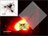 |
Fig. 1 Colour image: Haro 11 imaged with HST/NICMOS/NIC3 in the F160W filter (~H-band). Based on a 5 ks exposure obtained under a general observer programme 10902. North is up, east to the left. The scale is indicated with a solid white bar. The perturbed morphology is evident and demonstrates that the stellar mass distribution of Haro 11 is very asymmetric. Telltale merger features like sharp edges and tails are clearly visible. The apertures for the FLAMES/ARGUS and VIMOS/IFU spectra are indicated as grey semi-transparent rectangles. Greyscale image on the upper left: HST/ACS Hα image (Östlin et al. 2009) with the three knots |
Log of spectroscopic observations.
2. Observations and reductions
We make use of several spectroscopic observations of Haro 11 all obtained at the ESO telescopes in Chile; for a summary see Table 2. In addition we show images from the NASA/ESA Hubble Space Telescope (HST), obtained under general observer programmes 10575 and 10902 (PI Östlin).
2.1. Long-slit spectra with FORS2
Our long-slit spectra were taken with FORS2 (under ESO programme 071.B-0602) at moderate and low resolution, using two slit orientations on the galaxy, see Table 2 and Fig. 1. One, at position angle (PA) 57.5° passes through both knot and knot (hereafter referred to as slit  ); the other at PA 140° (hereafter referred to as slit ℬ) passes through knot ℬ and the galaxy’s apparent kinematical centre (see Fig. 1 and Hayes et al. 2007). We obtained spectra for both position angles using the high-resolution G1028z grism and a slit width of 0.7′′, and for slit only also using the lower resolution G600B and G600RI grisms. The higher resolution spectra cover ~7700−9400 Å, and include several transitions of the H i Paschen series, nebular lines such as [S iii]9069 and the Ca ii triplet. The lower resolution data cover the spectral region from 3330 Å to 8450 Å. The relatively narrow slit width was chosen to improve spectral resolution (resulting R ~ 4800 and 2000 for high- and low-resolution grisms, respectively). A number of template stars (of spectral type F8 to K2), to be used in the cross-correlation analysis, were also observed with the same set-up. The instrument resolution was measured from unresolved sky lines. We obtained and reduced the low-resolution spectra in a standard manner with wavelength calibration provided by arc lamp exposures.
The G1028z observations were designed to optimise subtraction of the strong sky emission from atmospheric OH and O2. For both slit positions, we took a number of identical exposures with the galaxy placed at different positions along the slit. We set the nodding step between two consecutive exposures to always have a different length from previous exposures, and in addition made sure that the step is always larger than the apparent size of the galaxy.
First, a constant background value was subtracted from each exposure, with the level determined between the OH lines at 8510 Å. Then adjacent pairs of exposures were subtracted from each other, each time scaling the subtracted frame, so that residuals from the OH and O2 lines were minimised. Wavelength calibration was carried out in two dimensions using OH sky lines in the non-subtracted frames, and wavelengths from Osterbrock et al. (1996). To remove pixel-to-pixel variations in the response of the CCD, we divided each pair-subtracted frame by a dome flatfield. We found that the OH and O2 lines varied somewhat differently from each other from exposure to exposure. They are, however, easy to separate. In the region of interest, O2 emission dominates the background between 8600 and 8720 Å, so we were able to perform scaling and subtraction for the two cases separately, and then spliced the spectra together again after flat-fielding. The spectra were registered and median combined to produce the final frames for use in the subsequent analysis. We extracted the spectra three detector rows at a time (0.̋75) and flux-calibrated by comparison with standard stars LTT 7379 and LTT 7987.
2.2. Integral field spectra with FLAMES/ARGUS
Integral field unit (IFU) spectroscopy was taken using the FLAMES integral field unit ARGUS, connected to the spectrograph GIRAFFE (Pasquini et al. 2002) under observing programme 074.B-0771. We used the  pix-1 scale with grating set-up LR8, giving a spectral coverage from 8200 to 9380 Å with spectral resolution R ≈ 10 400. The 22 × 14 lenslets result in a field of view of
  placed with the long side in east-west direction (see Fig. 1). Three spectral template stars (of spectral type K0II, K0III, G8Iab) were observed with the same set-up.
We reduced the data in the same manner as in Marquart et al. (2007), using the software and methods of Piskunov & Valenti (2002) for bias subtraction, flat-fielding, wavelength calibration, and optimised extraction of each spectrum. Sky emission was subtracted using simultaneously observed spectra from the separate 15 sky fibres (see e.g. Kaufer et al. 2003). As a consistency check, we integrated the spectra over the whole galaxy and derived the systemic velocity to be 6179 km s-1, in good agreement with previous results (cf. Table 1).
2.3. Integral field spectra with VIMOS
Haro 11 was also observed with the VIMOS IFU using the HR-blue grism in programme 74.B-0802 (PI Bergvall). These observations, originally designed for a different scientific purpose, were obtained at a pointing well outside the main body (15′′ to the NW, see Fig. 1), but contain velocity information on the ionised gas, which was deemed useful for the current investigation, and therefore we included these data in our analysis.
The VIMOS/IFU with HR-blue grism1 and scale  per fibre delivers a field of view of 27″ × 27″ over the wavelength range 4150–6200 Å. We detect [O iii]λλ4959,5007 and often also Hβ over most of the field of view. The spectral resolution is R ≈ 2550, verified by the width of sky lines in the spectrum. The IFU spectra results from a single 7200s integration. To remove cosmic rays in this single deep exposure, we first normalised each spectrum to the continuum near [O iii] and took the median of 5 × 5 pixels, constructing a binned spectral image with 3.̋3 resolution. Since VIMOS/IFU lack dedicated sky fibers, the sky level was estimated from a dedicated blank sky exposure of 1800s next to the target. Some regions of the IFU showed a significantly higher residual background level and were not included in the further analysis.
2.4. Fabry-Perot interferometry
Fabry-Perot interferometry was collected with CIGALE (Amram et al. 1991) mounted on the ESO 3.6-m telescope, under programme 63.N-0736, using an etalon with free spectral range (FSR) of 390 km s-1. The spatial sampling was 0.94′′/pixel. The etalon was scanned in 64 channels (each 6.1 km s-1 wide) for a total integration time of 3200 s. The data was reduced with the Adhoc (Boulesteix 1993) software, and a Gaussian smoothing of 1.̋5 was applied. The effective spectral resolution in the reduced data cube, as measured by the width of the instrument profile, is 29 km s-1 FWHM.
3. Stellar kinematics from the calcium triplet
Observing the stellar velocity field in metal-poor starbursting galaxies is very challenging because of intrinsically weak stellar absorption lines and contamination from ionised gas emission. In galaxies like Haro 11 with very strong emission line spectrum, the Balmer lines become completely emission dominated. The calcium triplet, which originates from photospheric absorption in red giants and red super giant stars, is one of very few practically accessible probes. However the calcium triplet lines are partly blended with Paschen lines, which needs to be dealt with before stellar velocities can be derived.
3.1. Removing Paschen emission lines
We subtracted the lines of the H i Paschen series from our FORS2 spectra, according to the scheme presented in Cumming et al. (2008). As a template for the higher order Paschen lines, we constructed a model profile by adding the profiles of the three strongest H i lines in our spectra that are not blended with the calcium triplet lines (Pa 10, 11 and 12). Where the signal-to-noise ratio was low, we used [S iii] λ9069 as a template.
We adjusted the width, flux, and velocity of the model lines to give the best subtraction around those Paschen lines, which do not blend with Ca ii absorption. Finally we masked the few other emission lines seen in the spectra, O iλ8446, [Cl ii] λ8579 and Fe iiλ8617. For the ARGUS spectra, we followed the same procedure for subtracting Paschen emission lines, using Pa 10 as the sole profile template because of the limited wavelength coverage.
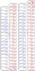 |
Fig. 2 Variation along the slit of the cross-correlation function (CCF, first and third columns) from fxcor and the [S iii] λ9069 line profile (second and fourth columns). The leftmost two columns show the results for slit ℬ and the rightmost columns the results for slit |
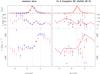 |
Fig. 3 Kinematical results along FORS2 slit ℬ showing (from upper to lower) the flux level, the line-of-sight velocity dispersion, and the heliocentric radial velocity (relative to the systemic velocity of 6175 km s-1). Zero on the abscissa is defined as the point where our two slits cross. The left panels show results for the [S iii] λ9069 (red open circles), and H i Paschen emission lines (weighted means of all measured lines; blue filled circles). The flux scale show the normalised strengths of the emission lines. The dotted vertical lines at 2′′ and 5′′ marks the position along the slit of knot ℬ, and where the slit crosses the loop of structures is referred to as the ear (see also Figs. 1 and 6). The dotted horizontal line in the σ-plot is arbitrarily put at 75 km s-1. The right panel shows at the top the spatial variation of the normalised continuum flux near the calcium triplet (orange), in arbitrary units. The red solid line repeats the [S iii] flux distribution from the left panel. The middle and lower panels show the derived stellar velocity dispersion and radial velocity, respectively. Again, the red solid line repeats the [S iii] results from the left panels. The results from cross-correlation is shown with orange squares and the pPXF is shown as magenta open circles. The grey triangles represent the extreme values derived (as described in Sect. 3.2) from the cross-correlation method when we take systematics in the Paschen emission line subtraction into account. At the distance of Haro 11, 10′′ corresponds to 4 kpc. |
3.2. Stellar kinematics from FORS2 slit spectra
We derived the stellar kinematics with cross-correlation of the cleaned spectra using FXCOR (based on Tonry & Davis 1979) and the same set of template stars as in Cumming et al. (2008). We followed the method of Östlin et al. (2007) for deriving the resulting errors in the velocity dispersion. Figure 2 shows how the cross-correlation function (CCF) peak and the [S iii] profiles vary along each slit. In the right panels of Figs. 3 and 4, we show the resulting stellar velocities (relative to the systemic velocity 6175 km s-1) and velocity dispersions (with orange squares plus error bars). Independently, we derived the velocities and dispersions using the penalised pixel-fitting (pPXF) method of Cappellari & Emsellem (2004) (shown as magenta circles in Figs. 3 and 4).
The derived velocities and velocity dispersions are subject to systematic errors from the Paschen line subtraction, in particular, where the Paschen emission is strong and the calcium triplet weak. In Fig 2 those CCFs for which the peak amplitude was below 0.25, or the Paschen subtraction was not deemed reliable, are shown in grey, and these points were discarded from the subsequent analysis. To quantify the effects of over- and under-subtraction of the Paschen lines, we additionally investigated two extreme cases:
-
(i)
We increased the Paschen line intensities as much as possiblewithout inducing artificial absorption features, all the whileadjusting the velocity dispersion and velocity of the nebular linemodel to allow the maximum intensity to be subtracted.
-
(ii)
In the other case, we instead kept the subtracted intensity as low as possible without leaving any residual emission features at the unencumbered Paschen lines, again letting the velocity and velocity dispersion take any values to assure this.
The spectra resulting from the two alternative subtractions were then cross-correlated as before. The results bracket the possible range of velocities allowed by the data, and give a good estimate of the maximum systematic errors. In Figs. 3 and 4 we show, with upwards and downwards triangles, the velocities and dispersions resulting from these extreme Paschen subtractions. The comparison with the pPXF results give further information about the systematics. Sometimes the differences are larger than those represented by the error bars, and other times smaller. In the latter case, the obtained result should be regarded as quite robust. The stellar velocities are found to be insensitive to the template star used in the cross-correlation, so we treat the data for the bright KO giant HD 164349 as representative.
For slit , we see that the stellar velocities and dispersions resulting from the two different methods (FXCOR and PPXF) and extreme Paschen subtractions agree very well, and hence the overall velocity and dispersion profile must be regarded as very reliable. For slit ℬ the agreement is worse, partly because the emission lines are stronger along this slit.
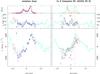 |
Fig. 4 Same as Fig. 3, but for slit |
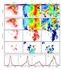 |
Fig. 5 Maps of the field of view of FLAMES/ARGUS showing the derived properties of the [S iii] λ9069 line. The tick marks have a spacing of 1′′. Upper row: results from a single component fit, from left to right: intensity in arbitrary logarithmic units (with the location of the 3 knots indicated with crosses), velocity and velocity dispersion. Since we find that over large areas, a single velocity component is insufficient to reproduce the line profile, we present an attempt to decompose the line by fitting multiple Gaussians. The number of components was chosen conservatively and additional components were only included when deemed necessary to produce a decent fit. The results are presented in the three middle rows. Lower row: examples of measured [S iii] line profiles (black solid line), and our multi-component fits to them (first: blue dotted, second: green dash-dotted, third: yellow dashed). The red solid line is the sum of the components. The x-axis indicates velocity, relative to the systemic velocity, in km s-1. The positions that correspond to the spectra are shown with numbers over-plotted on the panels above them. |
3.3. Stellar kinematics from FLAMES/ARGUS
After Paschen subtraction, we followed the procedure described in Marquart et al. (2007). However, poor signal to noise and strong Pa emission lines in many of the spaxels meant that we could not derive a detailed spatial map of the stellar velocities. After binning 2 × 2 we were able to determine the stellar velocity in the region around where the Paschen emission is relatively weak, finding good agreement with the FORS2 result. The only region where we get reliable velocity data, which was not covered by FORS2, is 2′′ south-east of knot . Here the stellar velocities are the same as those for gas (derived from [S iii]). We do not discuss the stellar kinematics from ARGUS further.
4. Ionised gas kinematics
Velocities for the ionised gas are calculated using rest wavelengths from van Hoof (1999) and (for [S iii] only) Hippelein & Muench (1981).
4.1. Gas kinematics along the FORS2 slits
The analysis of the FORS2 ionized gas velocities and their errors follow (Cumming et al. 2008). In general we use [S iii] λ9069, the strongest line in the G1028z spectra. Along slit position we also observed Hα with grism G600RI, which allows us to probe the velocities to somewhat larger radii than for [S iii], albeit with lower spectral resolution. The [S iii] emission line profiles are shown in Fig. 2 and it is obvious that they are non-Gaussian at many places. Since the ARGUS data has higher spectral resolution, we restrict our analysis of the detailed line shape to this data; see next subsection. In Figs. 3 and 4 we show the velocities and velocity dispersions for stars and gas derived from the assumption of a single Gaussian component. The regions coinciding with knots , ℬ, and have smaller velocity dispersion than the average of their surroundings.
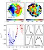 |
Fig. 6 Results from CIGALE Fabry-Perot Hα observations of Haro 11. Upper left: line-of-sight velocity (relative to the systemic velocity) with the scale (in km s-1) given by the colour bar beneath. The spatial scale is indicated in the corner and a single Hα flux contour (at ~5 × 10-15 erg s-1cm-2 arcsec-2) is over-plotted for reference. The solid black line shows the line along which the rotation curve (in the lower left panel) was extracted and the dashed lines indicate the ± 40deg wedge of points included. Upper right: velocity dispersion map. The same contour as in the first panel is over-plotted. The white circles mark the positions of knots |
4.2. ARGUS
We used [S iii] λ9069, the strongest emission line in our spectra from ARGUS, to derive spatially resolved kinematics of the ionised interstellar medium. The upper row of Fig. 5 shows maps of amplitude, velocity, and velocity dispersion resulting from a fit to the line using a single velocity component. Because the line shape at this spectral resolution is non-Gaussian over large regions of the field of view, we allowed for two additional degrees of freedom in the form of the parameters h3 and h4 from the Gauss-Hermite polynomials. They represent skewness and kurtosis (spikiness/boxiness), respectively, and generally allow the fitted velocity to better correspond to the peak of the line profile.
The [S iii] line shows a complex kinematic structure and several individual line profiles indicate the presence of multiple velocity components. We next decompose the [S iii] line profiles into several components by fitting multiple Gaussians in the regions where it is clear that the profile cannot be described by a single component. We use the smallest numbers of components deemed necessary from the shape of the line profile and the quality of the data. This means that for some pixels we have one component, for some two, and for others three. Even three components are sometimes insufficient (e.g. lower right panel labelled “4” in Fig. 5), but we refrain from fitting more than three profiles because of the ambiguity in the interpretation.
The line decomposition in some places reveal up to three dynamical components: how can we spatially make sense of these components? There is a principle problem of multi-component fits in that one needs to arrive at a spatially consistent identification and labelling. The question of whether a component at one place in the galaxy is related to a particular component in a nearby region is non-trivial as each component may vary spatially both in velocity, width, and amplitude. We use spatial continuity over several pixels as a criterion for manually deciding how to sort the components in an iterative fashion. This means that we tried to avoid discrete jumps in velocity and line width for a given component. Rows 2−4 in Fig. 5 show maps of the resulting kinematical components: the first component is wide spread over the field. The second component forms a kinematically cold structure that is well defined in space, intensity, velocity, and line width, and which we associate with the ear. The third component is somewhat more elusive. The first component represents everything that does not belong to the second or third component or when the line shape does not obviously require more than one component.
In addition to the sorting problem, there is another uncertainty that affects the velocities and dispersions shown in Fig. 5: multiple components can only be clearly identified if they have different amplitude or are separated in velocity by an amount comparable to the FWHM of the individual lines. This means that even where a single component may seem sufficient, there might in reality be several distinct regions projected along the line of sight. If the velocity separation and relative intensity of different components change, at some positions they may blend and two relatively narrow slightly separated components may be mistaken for a single broad one, leading to velocity and σ jumps.
4.3. CIGALE
The Hα velocity field from CIGALE was analysed by fitting a Gauss-Hermite polynomial to the line profiles in each pixel. The resulting velocity field (h1) and velocity dispersion (h2) are shown in Fig. 6. There is a good agreement with the [S iii] velocity field (Fig. 5). To allow a comparison with the results of Östlin et al. (1999, 2001), we have also extracted a rotation curve along the major axis defined by the new photometry presented in Micheva et al. (2010), where the shape of the K = 23 mag/arcsec2 isophote was fitted with a position angle PA = 103° and an inclination i = 47° (see Fig. 6). The line-of-sight Hα line widths are σ ≈ 60 km s-1 at and , and ~80 km s-1 at ℬ. The broadest lines are seen in the overlap region (i.e. approximately the point where the two FORS2 slits cross and where the ARGUS data reveals at least three velocity components in the [S iii]-line), and also 4′′ south of this region and in addition 2−3′′ north and east of .
4.4. VIMOS
In the VIMOS data, the Hβ, [O iii] λ4959, and λ5007 lines are detected in all binned pixels. We simultaneously fit the [O iii] lines with a single red-shifted Gaussian each, connected by the intensity ratio 1:3, a common width and a separation of Δλ = (5007−4959)(1 + vr/c) Å where vr is the fitted radial velocity. We independently fit the Hβ line with a single Gaussian.
The field of view of the VIMOS IFU was placed at a 45° angle north-west of knot ℬ. Since we are interested in how the gas velocity and line width changes with distance from the starburst, we collapsed the velocity field along the direction of slit B, resulting in a single set of velocity versus radius data; shown as black dots in Fig. 7. Scattered light could potentially be an issue with VIMOS IFU data (Monreal-Ibero et al. 2006), however, our pointing is far from the bright centre, which is well outside the field of view of VIMOS/IFU.
The Hβ data is quite noisy but on average the [O iii]/Hβ ratio is ~5, similar to that seen in the centre (Bergvall & Östlin 2002). We find that the Hβ velocities match those of the [O iii] lines within the uncertainties. Therefore we only further investigate the [O iii] lines. The stacked [O iii] lines show no apparent structure, such as asymmetries or double components. They are, however, significantly broader than the instrument profile, which we measured to be FWHMinstr = 124 km s-1 (or equivalently σinstr = 53 km s-1). In the high signal-to-noise bins, the raw width as determined from a Gaussian is σraw = 100 ± 10 km s-1, implying an instrument corrected line width of σ ≈ 85 ± 10 km s-1, i.e. very similar to the average value in the centre of 81 km s-1 (Östlin et al. 2001); see also Fig. 6. There is a weak decline in σ with increasing radius.
5. Results and analysis
Figures 3 and 4 show how the velocity, σ and flux vary along the FORS2 slits, for selected emission lines (left panels) and for Ca ii (right panels). The results for slit (Fig. 4) show a clear correspondence between the velocities and dispersions for gas and stars. The velocity curves are not identical, but overall, stars and gas have very similar kinematical properties. Slit ℬ adheres to this trend even if the poorer data makes it less obvious.
The ARGUS ionised gas velocity field, on closer inspection, showed evidence for multiple kinematical components, as discussed below. Also the stellar velocities may be multi-component in nature as hinted by the shape of some of the CCFs in Fig. 2, but the current data does not allow us to reliably investigate this further.
The similarity of the stellar and gaseous velocities suggest that they have a similar physical origin, namely virial motions. Whereas gas is known to be affected by feedback, this apparently has not affected the line core, perhaps because gas that is affected by feedback tends to become diluted and have low intensity. The motions of stars are, on the other hand, not affected by feedback.
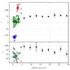 |
Fig. 7 Line-of-sight velocity of gaseous emission lines along PA −45°. Black dots are the [O iii] velocities and line-of-sight σ from our VIMOS data. The error bars for all points represent the spread (1σ) of the individual measurements within the radial bin, not the measurement error. Green, red, and blue dots correspond to the first, second, and third velocity component from the ARGUS analysis of the [S iii] line (cf. Fig. 5), as derived by a cut through the velocity field in the north-west direction. Small symbols represent individual spaxels and large symbols radial averages with error bars showing the spread. The scale is 0.4 kpc/arcsec. |
5.1. Analysis of the [SII] velocity field
The high spectral resolution of the ARGUS IFU-spectra allows us to have a closer look at the shape of a gaseous emission line. If one measures a line shape that is clearly the sum of multiple components with different velocities, it is safe to assume that they originate from physically distinct regions since it is hard to imagine a single region with two or more distinct bulk motions. This means that we have a handle on the third dimension of Haro 11, perpendicular to the plane of the sky.
Figure 5 shows the result and some examples of fitted line profiles. Several results emerge from this:
-
(1)
There is a main velocity component in the sense that it can beseen across the galaxy. There seems to be no indication of adiscontinuity as one would expect in a system that has not yetmerged. The decomposed line has its broadest(σ ≈ 90 km s-1) component ~1″ south-west of knot ℬ (see spectrum “2” in Fig. 5). This is also apparently the most dusty region (see Fig. 9). It is possible that the broad component giving rise to the high line width is in fact due to unresolved narrower components.
-
(2)
The second velocity component shows a near spatial coincidence with the ear (Fig. 1). It forms a high velocity component that is narrow in space and velocity (σ ~ 30 km s-1). It is likely a likely tidal arm, that was flung out in the merger, and which may be associated with the ear. In a less detailed investigation, the high velocities at the location of the ear could have been misinterpreted as due to rotation. Structures like this could easily be hiding in low spectral resolution studies of BCGs or merging galaxies, and highlight a potential pitfall in interpreting the kinematics of complex galaxies through low-resolution spectra. The kinematical information from VIMOS (see Fig. 7) support this interpretation. The velocities measured further to the north-west (Fig. 1) do not coincide with the high velocity of the second component, but instead joins smoothly with the first component. Hence, the ear is a spatially and kinematically distinct region. Figure 1 shows that the Hα emission in the ear is dominated by a chain of compact young star clusters, Adamo et al. (2010). Similar structures as the ear are seen in the Antennae (see Whitmore et al. 2010, and also Sect. 5.5 in this paper).
-
(3)
There is a third lower velocity component, mostly around knot A and the overlap region (position 3 in Fig. 5).
The Hα velocities probed by Cigale (Fig. 6) in general agree well with those from [S iii] although the spatial resolution is worse. The Hα line is markedly non-Gaussian over most of the galaxy, and is broadest in the overlap region.
5.2. Stellar kinematics and virial masses of knots , ℬ, and
The stellar velocities along slit shows a gradient of about 50 km s-1 kpc-1 (Fig. 4). The stellar velocity dispersion ranges between 60 and 150 km s-1 and largely follows that of the gas, peaking halfway between knots and (close to 0′′ on the abscissa, i.e. the overlap region). At this point the ionised gas spectrum from all instruments (CIGALE, ARGUS, FORS2) is markedly multi-component. Also the CCF structure is suggestive of multiple stellar components, and this is the most likely explanation for the very high stellar velocity dispersion found.
Both the stellar continuum and the absorption line equivalent width of the Ca ii triplet are strongest at the position of knot , where the velocity dispersion of gas and stars show a local minimum of σ ≈ 50 ± 10 km s-1. knot is very compact and unresolved if not viewed with the HST or adaptive optics. Using the baolab package (Larsen 1999) and the HST/ACS/HRC/F814W image, we find the light distribution to be best fitted with a King profile with effective radius of reff = 40 ± 10 pc. This indicates a virial mass for knot of 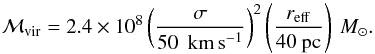 (1)Adamo et al. (2010) used SED fitting to estimate an order of magnitude lower stellar mass, which however was based on the assumption that was a point source and therefore grossly underestimated the total flux.
In HST images, knot is resolved into a group of bright star clusters. The size of the group is reff ≈ 200 pc and the velocity dispersion σ ≈ 50 km s-1. Hence the dynamical mass of the complex making up knot is ℳvir ~ 109 M⊙.
For knot ℬ we measure σ ≈ 80 km s-1, although it is more uncertain than for and because of the very bright emission lines. With a size of reff ≈ 140 pc the mass is of the order ~2 × 10⁹ M⊙.
The velocity dispersion (both for gas and stars) have local minima at the positions of knots and bright clusters. This is understandable since in these kinds of cases the light is dominated by the knot in question and the measured line width is strongly biased by local conditions in the knot, whereas in a random position, the line profile has (often unresolved) contributions from many velocity components along the line of sight. It does not imply that the knots are necessarily dynamically cooler.
Comparing the stellar and nebular gas velocity field, it is striking how similar they are on average. While we do not have the same possibility to resolve the stellar velocity field into multiple components, the similarities indicate that Ca ii and nebular lines trace the dynamics of the system in a similar way. Stars are not subject to outflows and, hence, while there may well be outflow components present in the nebular spectrum at many points, they do not dominate the local fluxes.
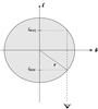 |
Fig. 8 Schematic illustration of relevance for the discussion in 5.3. An observer sees the galaxy at an impact parameter b along the line of sight (dashed line). The line of sight intersects the hypothetical galaxy between lmin and lmax |
5.3. The VIMOS far out velocity field
How do we explain the VIMOS results showing a flat velocity curve and an emission line width of σlos ~ 80 km s-1 at galactocentric distances ≥ 10 kpc? First, this value is similar to the average found for a one-component fit to the nebular gas (and the stars) in the more central regions. The spectral resolution of the VIMOS spectra and the S/N do not allow for a multi-component analysis. Below we discuss a few alternative explanations for the broad lines.
Thermal broadening: thermal broadening can be ruled out since the implied temperature (~106 K) would be unrealistic for a gas showing [O iii] in emission. The [O iii] electron temperature in the centre (where the line is equally broad) is ~104 K (Bergvall & Östlin 2002). Hence, the line broadening must be macroscopic and due to bulk motions.
Rotational broadening: if the far reaches of Haro 11 were a rotating disk, the line profile would be broadened by the fact that the rotational velocity has a different sign and amplitude along the line of sight. Assume we view the galaxy at some impact parameter b according to Fig. 8 and that the galaxy has a constant rotational speed vrot, which we observe at an inclination i. The observed velocity is vobs = vrotsin(i) and from Fig. 7 we find that vobs = 50 km s-1. At b ≫ 0, the line would be made up by components with velocities ranging from  km s-1 (at l = lmin and lmax) to vobs at l = 0, and the induced line broadening would be
 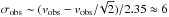 km s-1 (where the factor 1 / 2.35 comes from the transformation of FWHM to σ). Hence, rotation gives a negligible contribution to the line width.
A radial outflow: a scenario that is compatible with a flat velocity gradient and broad emission lines is a uniform radial expansion, since this does not affect the velocity centroid (i.e. the rotation curve), but broadens the line. A spectrum at a projected galactocentric distance b would sample velocities with line-of-sight components 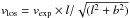 from lmin to lmax, see Fig. 8. At l = 0, the expansion is purely transversal, whereas l< 0 and l> 0 produce blue- and red-shifted components, respectively, which broaden the line. The resulting broadening in FWHM would be approximately vexp, which therefore would have to be ~200 km s-1 to explain the width of the line. The line width would be expected to get narrower at larger radii and there is indeed a weak trend in that direction.
However, a real outflow is unlikely to be spherically symmetric. For instance, Johnson et al. (2012) investigated the nearby dwarf galaxy NGC 1569 in ionised gas and Hi, finding very extended and irregular bipolar velocity structures. If the far out velocity field in Haro 11 is due to outflows, it would be a coincidence that the VIMOS FOV happened to capture them. Kunth et al. (1998) found evidence for an outflow (of neutral gas) with 58 km s-1 from HST/GHRS spectroscopy in a pointing towards the centre of Haro 11. Additional sight lines were probed by Na absorption in Sandberg et al. (2013) who found an outflow of 44 km s-1 towards ℬ, but an inflow of 27 km s-1 towards . In conclusion, there is no evidence for a galaxy-wide radial outflow of the magnitude needed to explain the halo line width.
Turbulence from feedback: it has been debated whether emission line widths are due to virial motions or turbulence created through feedback from star formation (Terlevich & Melnick 1981; Green et al. 2010; Moiseev & Lozinskaya 2012). The fact that stellar and gas velocity dispersions tend to agree in Haro 11 argues against turbulent feedback driving the gas velocity dispersion. Moreover, the mechanical energy output of an instantaneous starburst peaks at about 20 Myr (Starburst99, Leitherer et al. 1999). In their analysis of the luminous star cluster population, Adamo et al. (2010) found that the star formation rate in Haro 11 started to increase rapidly 20 Myr ago. Hence, the current starburst has had limited time to transport mechanical energy out into the halo. For a scale of 10 kpc and a timescale of 10 Myr, the implied velocity is 1000 km s-1. We see no indications of a wind at this speed, and hence the line width is unlikely to have been produced purely by feedback.
Virial motions: we are left with the most plausible explanation that the line width is mainly due to macroscopic bulk motions of the ions. We can then use the clouds as tracers of the gravitational potential and Eq. (1) to get an order of magnitude dynamical mass estimate of ~1011 M⊙. The rotational velocity (~50 / sin(i) km s-1 at r = 12 kpc) provides another 5 × 10⁹/ sin2(i) M⊙, but is negligible in this context, and the “halo” of Haro 11 would be dominated by velocity dispersion. This assumes dynamical equilibrium and isotropic velocity dispersion, both which are questionable for a merging system like Haro 11, but the order of magnitude dynamical mass should nevertheless be 1011 M⊙ in this scenario. If the merging galaxies came in on parabolic orbits, pre-virialisation velocities are a factor of  higher and the inferred virial mass would be a factor of 2 too high.
To conclude, Haro 11 is rotating to the largest scales we can probe, and the rotationally supported mass is, under the assumption of circular motions, ~1010 M⊙. The emission lines in the halo region are broad, σ ~ 80 km s-1. We find that the line width is likely due to bulk motions indicating a mass of ~1011 M⊙.
5.4. Stellar and dynamical masses
From multi-wavelength data it is possible to estimate the mass in stars through a comparison with spectral evolutionary synthesis models, under the assumption of an initial mass function (IMF) and a certain star formation history. This is commonly referred to as stellar mass. While the resulting age and star formation history is subject to degeneracies, the stellar mass is often more robust (for reasons discussed in e.g. Östlin et al. 2001).
Östlin et al. (2001) found that for radii r> 1 kpc, the stellar mass distribution in Haro 11 could not be supported by rotation. Only by assuming that the observed Hα velocity dispersion trace mass could the dynamical and stellar masses be reconciled. Then the inferred dynamical mass is 1.9 × 10¹⁰ M⊙ for an effective radius of 2.8 kpc and σ = 81 km s-1.
Here we also make use of the stellar population modelling of Haro 11 performed in Hayes et al. (2007). In that paper, the stellar population was modelled in a spatially resolved fashion using HST multi-band imaging from 1500 Å to the I-band, and with two populations (one young and one old) plus one ionised gas component. The underlying assumptions were that both populations are single stellar populations, calculated with Starburst99 and Geneva tracks with metallicity Z = 0.004 and Salpeter (1955) IMF. If we integrate the stellar mass from the reference position where the slits cross (r = 0) and out to r = 10′′ , we find a total stellar mass of 2.4 × 10¹⁰ M⊙. Half the quoted mass is contributed by the inner r< 3′′, which encompasses the three main knots. The stellar mass estimate is primarily sensitive to the assumed low-mass slope and cut-off of the IMF. For more realistic IMFs where the slope flattens a low mass (e.g. Scalo 1986; Chabrier 2003) this estimate should be reduced to about 60% of the quoted value, or ≈ 1.4 × 10¹⁰ M⊙. These estimates are of the same order as those by Östlin et al. (2001) (M⋆ = 1.6 × 10¹⁰ M⊙) and Madden et al. (2014) (M⋆ = 1.7 × 10¹⁰ M⊙), both studies using independent data.
We see a sharp velocity gradient along slit from −6′′ to + 4′′ (i.e. a total extent of 4 kpc) over which the velocity varies monotonically with 200 km s-1. Interpreting this in terms of rotation gives a rotationally supported mass of 4.6 × 10⁹/ sin2(i) M⊙, which for i> 30° is smaller than the mass inferred from the line width (if using the same radius). The inclination is not well constrained, but rotation likely gives a significant contribution to the central (r ≤ 10′′) region. Further out, we can follow the Hα kinematics along slit from −12′′ to + 16′′ (a total scale of 11 kpc). The velocities change the slope on both sides, but the gradients are about equally steep, and the same is observed in the CIGALE velocity field (Fig. 6).
Hence the velocity field in this ongoing merger is complex. If the velocity gradients are interpreted in terms of gravitational motions, there also seems to be ample dynamical mass outside the central 4 kpc. The velocity amplitudes and σ are the same as in the centre, but the spatial extent is almost three times larger. With this assumption, the total dynamical mass for the Haro 11 system may approach 1011 M⊙. This is close to the value inferred from the VIMOS far out velocity field discussed in the previous subsection
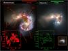 |
Fig. 9 Antennae (left, credit STScI and B. Whitmore) and Haro 11 (right, Adamo et al. 2010, credit ESO/ESA/Hubble and NASA) put next to each other. The Antennae image has been rotated to the same apparent orientation as Haro 11 (which is shown as N up E left) and the images have been scaled so that the two systems look equally big on screen, for ease of comparison. The physical scale for the image of each system is shown with the red and green bars. In the image of Haro 11, we labelled the three main knots according to their common designation A, B, and C (Hayes et al. 2007). In the image of the Antenna we point out with arrows and roman numerals some regions of similarity, which are discussed in text. In the lower right inset we show the image of Haro 11 at the same physical scale of the Antennae. The image of Haro 11 is a composite of observations from HST/ACS (filters F435W, F550W, F814W) and VLT/NACO (Ks). The inset plot in red (lower left) show the position-velocity (PV) diagram for the Antennae (Amram et al. 1992) and the green inset to the right shows the same for Haro 11(this work). The PV diagrams have been extracted through the two nuclei in the Antennae and the corresponding for Haro 11 as seen in Fig. 9, i.e. knots |
5.5. Haro 11 – a denser version of the Antennae
Haro 11 presents a very rich and complex velocity structure. This comes as no surprise given the morphological features seen in the 1.6 μm HST/NICMOS image (Fig. 1). However, Haro 11 presents yet more intriguing features. Comparing it to the Antennae galaxies reveals striking similarities. We demonstrate this in Fig. 9 where the HST images of the Antennae2 have been rotated and scaled to the same apparent orientation and size as Haro 11. On detailed inspection they almost look like copies, and bright irregular features and dust lanes in Haro 11 have close counterparts at the same apparent place in the Antennae and vice versa.
In Fig. 9 we highlight, using roman numerals, some conspicuous features, which are also discussed below: both galaxies present distinct edges in the underlying stellar distribution (I). Dust streaks that in the reference system of Haro 11 runs horizontally north of knot (II). A dusty Hα-bright region at ℬ (III). The region, which is called in Haro 11, is bright in Hα and has many optically bright and blue star clusters SE of it (IV). A faint tidal feature south-east of (V). An optically bright compact nucleus with dust lanes leading into it (VI). Also the ear in Haro 11 may have its analogue in the Antennae system (see e.g. Sect. 8 in Whitmore et al. 2010). Of course, there are differences too: knot is a complex of star clusters rather than a nucleus as in the Antennae, and Haro 11 lack extended tidal tails (see below). Nevertheless, the striking similarity of the two systems suggest a similar origin. The mergers appear equally advanced and have presumably been created by progenitor galaxies that are similar to both systems and that have had similar orbits with respect to each other. However, despite the striking similarities there is one important difference: Haro 11 is physically four times smaller than the Antennae.
The ionised gas velocity field of the Antennae was studied by Amram et al. (1992) where they used CIGALE, i.e. the same Fabry-Perot interferometer as in this work, to study the Hα line. The smaller distance and larger physical size allow for greater detail to be seen in the Antennae, so we compare gross properties (in the reference system of Haro 11). The region around in both galaxies show low velocity, the region around have significantly higher velocities, with ℬ being intermediate. Hence, the image projected on the sky plane is similar in both galaxies and the relative motions. Amram et al. (1992) showed a position-velocity (PV) diagram, extracted along the line joining the two nuclei, i.e. corresponding slit . We extracted a PV diagram from our CIGALE data cube along this direction and compare it with that of Antennae in Fig. 9. Again, the nearer distance to Antennae allows for more detail and a larger number of velocity points to be extracted, but overall the two PV diagrams are strikingly similar: they share the same overall shape and have the same velocity amplitudes (Δv ≈ 250 km s-1). The recent evolution of the SFR in the two galaxies also appears to be similar. From studying the ages and masses of young star clusters, Adamo et al. (2010) find that the SFR in Haro 11 has increased by a factor of 50 over the last 40 Myr. This corresponds to the estimated time of the 2nd pericentre passage of the merging galaxies in the Antennae after which the SFR has increased with a factor of 40 (Karl et al. 2010; Whitmore et al. 2007). Hence the timescales for the two mergers seems to be similar.
While knots and are separated by 2 kpc, and the nuclei in Antennae by 8 kpc (indicating a factor of 4 difference in size), the PV diagram in Haro 11 appears relatively more stretched. The distance between the extreme velocity values is 3.7 kpc in Haro 11and 7.6 in Antennae. This is because in Haro 11 and do not lie at the extreme values, but the velocity curve continues with the same shape beyond them. This is also obvious in Figs. 6 and 4, hence, Haro 11 is more compact in position space than in velocity space. We determine the velocity gradient is ~2.2 times steeper in Haro 11 taking into account that the beam smearing is larger for the more distant Haro 11. The dynamical mass and density of a system scales as, i.e.  The morphological similarity suggests that inclinations are similar for Haro 11 and the Antennae. Therefore our results suggest that the mass density in the central parts of Haro 11 is 2.22 ~ 5 times higher than that of the Antennae. Of course, given the non-equilibrium nature of mergers and the uncertainty of inclinations one should not take masses at face value, but the physical compactness of Haro 11 in any case argues for a higher density as compared to Antennae.
The star formation rate density is known to, on average, scale with the gas surface density as  (Kennicutt 1998). Since Σ = ρr the difference in surface density is again 2.2 and, hence, ΣSFR should be a factor of 2.21.4 = 3 higher in Haro 11, if the gas mass fraction is similar in the two systems.
The total star formation rate, SFR = r2ΣSFR, and we thus expect the total star formation rate of the Antennae to be 2.22/ 2.21.4 = 1.6 times that of Haro 11. Hayes et al. (2007) quote a probable SFR in the range 20 to 25 M⊙ yr-1 and Madden et al. (2014) finds 29 for Haro 11, whereas Karl et al. (2010) compile various estimates for the Antennae in the range 10 to 20 M⊙ yr-1. The Hα luminosity (uncorrected for extinction) is about three times higher in Haro 11 and the IRAS 60 μm luminosity is a factor of 2 higher (based on the values in NED). Hence Haro 11 seems to be forming stars at 2−3 times the rate of the Antennae, contrary to the expectation from the mass scaling.
To get a proxy for the stellar mass ratio of the two galaxy systems, we consider the K-band luminosities. NED gives Ks = 7.2 for the Antennae, or (for m − M = 31.9) MK = −24.7, while Haro 11 has MK = −22.9 (Bergvall & Östlin 2002). Hence the K-band luminosity of the Antennae is five times higher than that of Haro 11, and the stellar mass is likely at least ten times higher if one accounts for the fact that Antennae is more dusty and that Haro 11 due to its a stronger starburst should have lower M/LK. Hence, the specific star formation rate is at least 20 times higher in Haro 11 than in the Antennae.
The formation of tidal tails in mergers have been investigated in several simulation studies. Early claims that the absence of tails indicated very high dark matter fractions (Dubinski et al. 1996) were countered by Springel & White (1999), who showed that tails can be produced for high dark matter fractions provided the halo spin is sufficiently high. Hence the progenitor galaxies of the Haro 11 merger may have had smaller angular momentum or less extended dark haloes than the Antennae progenitors, both options suggesting more compact participating galaxies in Haro 11. A retrograde merger would also lead to weaker tails, but this explanation is unlikely in the case of Haro 11 given the close similarity with the Antennae, which has been successfully modelled with a pro-grade encounter (e.g. Karl et al. 2010). Certainly, dedicated hydrodynamical simulations would be key to better understand Haro 11.
Other merging systems do not possess such obvious apparent similarity as Haro 11 and Antennae. Arp 299 has a somewhat similar morphology. It is halfway in size between Haro 11 and Antennae and has a FIR luminosity 0.4 dex higher than Haro 11. Hence the SFR surface densities in Haro 11 and Arp 299 are comparable. While there is an abundance of gas in Haro 11 detected through various tracers it is remarkably devoid of cold Hi (Bergvall et al. 2000; MacHattie et al. 2014). The SFR per unit mass is very high in Haro 11 and Östlin et al. (1999) estimated that the mass of ionised gas in Haro 11 could be as high as 109 M⊙. The detection of [OIII] lines so far out suggest that the galaxy may be density bounded, which would be consistent with the claimed direct detection of Lyman continuum radiation (Bergvall et al. 2006; Grimes et al. 2007; Leitet et al. 2011).
To conclude, the morphological and kinematical properties of Haro 11 and the Antennae are stunningly similar, with the exception that the physical size of Haro 11 is a factor of ~4 smaller and the implied mass density roughly five times higher. The star formation rate is twice as high in Haro 11, which implies that the star formation efficiency is higher in Haro 11.
5.6. On the origin of the line width
It has long been known that the ionised gas follow a relation between the line width σ and the emission line strength of e.g. Hβ (Terlevich & Melnick 1981). The reason for this relation has been discussed over the years, and its discoverers have argued that it originates in virial motions. This has been challenged by others (Green et al. 2010; Moiseev & Lozinskaya 2012), however, who argue that the relation with the emission line luminosity, hence star formation rate, indicates that star formation itself, through feedback, broadens the line. In the current context, this question is important as we have used the line width to estimate masses. Feedback is of course also present in Haro 11 and similar luminous BCGs, but the question is whether feedback can produce lines with σ ~ 80 km s-1, i.e. affecting the bulk motions of the ionised gas rather than just producing broad low-intensity wings. Any matter in a galaxy must respond to the gravitational potential and in non-rotating systems, the line width always has a component from virial motions. In Haro 11 it is evident from this work, that the broad lines may be composed of many discrete velocity components and, what could be wrongly interpreted as a very turbulent ISM, is in fact a collection of moderately broad lines, which it takes high spectral and spatial resolution plus high signal to noise to reveal. The BCGs that so far have their stellar motions investigated through calcium triplet observations show that the H ii and stellar line widths are remarkably similar on a global scale (Östlin et al. 2004; Marquart et al. 2007; Cumming et al. 2008, this work). The motions of these predominantly young stars are not affected by feedback and they must have been born with this velocity dispersion. Hence, the ionised gas velocity dispersion must also be dominated by gravitation.
Studies of the evolution of the emission line width σ and σ/vrot show both increase with increasing red shift (e.g. Wisnioski et al. 2015). This can be intepreted as due to increased gas mass fractions, requiring higher σ to be stable, according to the Toomre criterion (Toomre 1964). Therefore we must conclude that the H ii line width seen in Haro 11 and similar systems to a large extent must be of gravitational origin. Numerical simulations (e.g. Bournaud et al. 2014) also show that turbulence drives star formation and not vice versa. The lines are not broad because of feedback from strong star formation, it is the turbulent medium that (by increasing the pressure and the Jeans mass) increases the star formation rate.
6. Conclusions
We have investigated the kimematics of ionised gas and stars in Haro 11, a luminous blue compact galaxy. Haro 11 hosts a very strong starburst in terms of specific star formation rate (or equivalently, birthrate b-parameter), and is also one of the nearest galaxies that match z ~ 3 Lyman break galaxies in terms of far UV luminosity and surface brightness. The kinematical data have been collected with the ESO VLT and 3.6 m telescopes. We also make use of imaging data from the Hubble Space Telescope.
We find that the stellar and ionised gas kinematics to first order agree very well, both showing the same large scale features and similar velocity dispersions. Hence, wherever we can trace their motions, stars are moving in similar directions and amplitude as the ionised gas. This implies that the bulk of the ionised gas emission arises from gas whose velocities are governed by gravitational motions. The irregularities in the velocity field must hence be attributed to real dynamical disturbances, providing further evidence that Haro 11 is a bona fide merger. This interpretation is also supported by the morphology, exemplified by the deep HST/NICMOS image showing telltale merger signs. The similar velocity dispersions in stars and gas also suggests that the Hα line width is primarily caused by virial motions. This suggests that emission lines provide a good probe of the kinematical state of dwarf starbursts, near and far.
When analysing the ionised gas velocity field at higher spectral resolution with integral field spectroscopy, we find several examples of double and triple line profiles. These components can only be resolved with high spectral resolution. We find high- and low-velocity components, however, which make a small contribution to the total intensity and which would therefore be missed by low-resolution spectroscopy. We used continuity arguments to associate the multiple line profiles with kinematical components. Notably, we find an elongated, kinematically cold, red-shifted arm.
Using an off-centre IFU observation, we can trace the ionised gas ([O iii] and Hβ) kinematics to large radii (r> 10 kpc), where we find a flat velocity curve offset from the centre with just 50 km s-1. The line width is the same as in the centre. We discuss various alternative explanations for the outer velocity field, such as outflows and turbulence, but favour an interpretation where the outer halo is slowly rotating but mainly supported by velocity dispersion, implying a total dynamical mass of 1011 M⊙.
We finally compare Haro 11 to the famous Antennae system and find stunning similarities. Haro 11 appears to be a more compact version of the Antenna, but otherwise shows very similar central morphology and kinematics. The Antennae is ten times more massive than Haro 11, but only forms stars at half the rate. One important difference is that Haro 11 lacks extended tidal arms, which may be due to more compact (denser) galaxies participating in the merger.
This is the old HR-blue grism. The new HR-blue grism has lower spectral resolution and a different wavelength range.
STScI News Release Number: STScI-2006-46, see: http://hubblesite.org/newscenter/archive/releases/2006/46
Acknowledgments
We thank a number of unnamed colleagues for interesting discussions. G.Ö. is a Royal Swedish Academy of Science research fellow (supported by a grant from the Knut & Alice Wallenbergs foundation). This work was supported by the Swedish Research Council and the Swedish National Space Board. This research has made use of the NASA/IPAC Extragalactic Database (NED), which is operated by the Jet Propulsion Laboratory, California Institute of Technology, under contract with the National Aeronautics and Space Administration. This research has made use of NASA’s Astrophysics Data System.
References
- Adamo, A., Östlin, G., Zackrisson, E., et al. 2010, MNRAS, 407, 870 [NASA ADS] [CrossRef] [Google Scholar]
- Adamo, A., Östlin, G., & Zackrisson, E. 2011, MNRAS, 417, 1904 [NASA ADS] [CrossRef] [Google Scholar]
- Amram, P., Boulesteix, J., Georgelin, Y. M., et al. 1991, The Messenger, 64, 44 [NASA ADS] [Google Scholar]
- Amram, P., Marcelin, M., Boulesteix, J., & Le Coarer, E. 1992, A&A, 266, 106 [NASA ADS] [Google Scholar]
- Bergvall, N., & Östlin, G. 2002, A&A, 390, 891 [NASA ADS] [CrossRef] [EDP Sciences] [Google Scholar]
- Bergvall, N., Masegosa, J., Östlin, G., & Cernicharo, J. 2000, A&A, 359, 41 [NASA ADS] [Google Scholar]
- Bergvall, N., Zackrisson, E., Andersson, B.-G., et al. 2006, A&A, 448, 513 [NASA ADS] [CrossRef] [EDP Sciences] [Google Scholar]
- Blanton, M. R., Hogg, D. W., Bahcall, N. A., et al. 2003, ApJ, 592, 819 [NASA ADS] [CrossRef] [Google Scholar]
- Boulesteix, J. 1993, ADHOC reference manual (Publications de l’Observatoire de Marseille) [Google Scholar]
- Bournaud, F., Perret, V., Renaud, F., et al. 2014, ApJ, 780, 57 [NASA ADS] [CrossRef] [EDP Sciences] [Google Scholar]
- Cappellari, M., & Emsellem, E. 2004, PASP, 116, 138 [NASA ADS] [CrossRef] [Google Scholar]
- Chabrier, G. 2003, PASP, 115, 763 [NASA ADS] [CrossRef] [Google Scholar]
- Cumming, R. J., Fathi, K., Östlin, G., et al. 2008, A&A, 479, 725 [NASA ADS] [CrossRef] [EDP Sciences] [Google Scholar]
- Dubinski, J., Mihos, J. C., & Hernquist, L. 1996, ApJ, 462, 576 [NASA ADS] [CrossRef] [Google Scholar]
- Gallego, J., Zamorano, J., Aragon-Salamanca, A., & Rego, M. 1995, ApJ, 455, L1 [NASA ADS] [CrossRef] [Google Scholar]
- Gil de Paz, A., Madore, B. F., & Pevunova, O. 2003, ApJS, 147, 29 [NASA ADS] [CrossRef] [Google Scholar]
- Gonçalves, T. S., Basu-Zych, A., Overzier, R., et al. 2010, ApJ, 724, 1373 [NASA ADS] [CrossRef] [Google Scholar]
- Green, A. W., Glazebrook, K., McGregor, P. J., et al. 2010, Nature, 467, 684 [NASA ADS] [CrossRef] [Google Scholar]
- Grimes, J. P., Heckman, T., Hoopes, C., et al. 2006, ApJ, 648, 310 [NASA ADS] [CrossRef] [Google Scholar]
- Grimes, J. P., Heckman, T., Strickland, D., et al. 2007, ApJ, 668, 891 [NASA ADS] [CrossRef] [Google Scholar]
- Hayes, M., Östlin, G., Atek, H., et al. 2007, MNRAS, 382, 1465 [NASA ADS] [Google Scholar]
- Heckman, T. M., Hoopes, C. G., Seibert, M., et al. 2005, ApJ, 619, L35 [NASA ADS] [CrossRef] [Google Scholar]
- Hippelein, H., & Muench, G. 1981, A&A, 95, 100 [NASA ADS] [Google Scholar]
- Hoopes, C. G., Heckman, T. M., Salim, S., et al. 2007, ApJS, 173, 441 [NASA ADS] [CrossRef] [Google Scholar]
- James, B. L., Tsamis, Y. G., Walsh, J. R., Barlow, M. J., & Westmoquette, M. S. 2013, MNRAS, 430, 2097 [NASA ADS] [CrossRef] [Google Scholar]
- Johnson, M., Hunter, D. A., Oh, S.-H., et al. 2012, AJ, 144, 152 [NASA ADS] [CrossRef] [Google Scholar]
- Karl, S. J., Naab, T., Johansson, P. H., et al. 2010, ApJ, 715, L88 [NASA ADS] [CrossRef] [Google Scholar]
- Kaufer, A., Pasquini, L., Castillo, R., Schmutzer, R., & Smoker, J. 2003, The Messenger, 113, 15 [NASA ADS] [Google Scholar]
- Kennicutt, Jr., R. C., 1998, ARA&A, 36, 189 [Google Scholar]
- Kobulnicky, H. A., & Gebhardt, K. 2000, AJ, 119, 1608 [Google Scholar]
- Kochanek, C. S., Pahre, M. A., Falco, E. E., et al. 2001, ApJ, 560, 566 [NASA ADS] [CrossRef] [Google Scholar]
- Kunth, D., & Östlin, G. 2000, A&ARv, 10, 1 [NASA ADS] [CrossRef] [Google Scholar]
- Kunth, D., Mas-Hesse, J. M., Terlevich, E., et al. 1998, A&A, 334, 11 [NASA ADS] [Google Scholar]
- Larsen, S. S. 1999, A&AS, 139, 393 [NASA ADS] [CrossRef] [EDP Sciences] [Google Scholar]
- Leitet, E., Bergvall, N., Piskunov, N., & Andersson, B.-G. 2011, A&A, 532, A107 [NASA ADS] [CrossRef] [EDP Sciences] [Google Scholar]
- Leitherer, C., Schaerer, D., Goldader, J. D., et al. 1999, ApJS, 123, 3 [NASA ADS] [CrossRef] [Google Scholar]
- MacHattie, J. A., Irwin, J. A., Madden, S. C., Cormier, D., & Rémy-Ruyer, A. 2014, MNRAS, 438, L66 [NASA ADS] [CrossRef] [Google Scholar]
- Madden, S. C., Rémy-Ruyer, A., Galametz, M., et al. 2014, PASP, 126, 1079 [CrossRef] [Google Scholar]
- Marquart, T., Fathi, K., Östlin, G., et al. 2007, A&A, 474, L9 [NASA ADS] [CrossRef] [EDP Sciences] [Google Scholar]
- Micheva, G., Zackrisson, E., Östlin, G., Bergvall, N., & Pursimo, T. 2010, MNRAS, 405, 1203 [NASA ADS] [Google Scholar]
- Micheva, G., Östlin, G., Bergvall, N., et al. 2013a, MNRAS, 431, 102 [NASA ADS] [CrossRef] [Google Scholar]
- Micheva, G., Östlin, G., Zackrisson, E., et al. 2013b, A&A, 556, A10 [NASA ADS] [CrossRef] [EDP Sciences] [Google Scholar]
- Moiseev, A. V., & Lozinskaya, T. A. 2012, MNRAS, 423, 1831 [NASA ADS] [CrossRef] [Google Scholar]
- Monreal-Ibero, A., Roth, M. M., Schönberner, D., Steffen, M., & Böhm, P. 2006, New A Rev., 50, 426 [Google Scholar]
- Nagamine, K., Springel, V., Hernquist, L., & Machacek, M. 2004, MNRAS, 350, 385 [NASA ADS] [CrossRef] [Google Scholar]
- Night, C., Nagamine, K., Springel, V., & Hernquist, L. 2006, MNRAS, 366, 705 [NASA ADS] [CrossRef] [Google Scholar]
- Osterbrock, D. E., Fulbright, J. P., Martel, A. R., et al. 1996, PASP, 108, 277 [NASA ADS] [CrossRef] [Google Scholar]
- Östlin, G., Amram, P., Masegosa, J., Bergvall, N., & Boulesteix, J. 1999, A&AS, 137, 419 [NASA ADS] [CrossRef] [EDP Sciences] [Google Scholar]
- Östlin, G., Amram, P., Bergvall, N., et al. 2001, A&A, 374, 800 [NASA ADS] [CrossRef] [EDP Sciences] [Google Scholar]
- Östlin, G., Cumming, R. J., Amram, P., et al. 2004, A&A, 419, L43 [NASA ADS] [CrossRef] [EDP Sciences] [Google Scholar]
- Östlin, G., Cumming, R. J., & Bergvall, N. 2007, A&A, 461, 471 [NASA ADS] [CrossRef] [EDP Sciences] [Google Scholar]
- Östlin, G., Hayes, M., Kunth, D., et al. 2009, AJ, 138, 923 [NASA ADS] [CrossRef] [Google Scholar]
- Overzier, R. A., Heckman, T. M., Kauffmann, G., et al. 2008, ApJ, 677, 37 [NASA ADS] [CrossRef] [Google Scholar]
- Overzier, R. A., Heckman, T. M., Tremonti, C., et al. 2009, ApJ, 706, 203 [NASA ADS] [CrossRef] [Google Scholar]
- Pasquini, L., Avila, G., Blecha, A., et al. 2002, The Messenger, 110, 1 [NASA ADS] [Google Scholar]
- Pérez-Gallego, J., Guzmán, R., Castillo-Morales, A., et al. 2011, MNRAS, 418, 2350 [NASA ADS] [CrossRef] [Google Scholar]
- Piskunov, N. E., & Valenti, J. A. 2002, A&A, 385, 1095 [NASA ADS] [CrossRef] [EDP Sciences] [Google Scholar]
- Puech, M., Hammer, F., Flores, H., Östlin, G., & Marquart, T. 2006, A&A, 455, 119 [NASA ADS] [CrossRef] [EDP Sciences] [Google Scholar]
- Salpeter, E. E. 1955, ApJ, 121, 161 [Google Scholar]
- Sandberg, A., Östlin, G., Hayes, M., et al. 2013, A&A, 552, A95 [NASA ADS] [CrossRef] [EDP Sciences] [Google Scholar]
- Scalo, J. M. 1986, Fund. Cosmic Phys., 11, 1 [NASA ADS] [EDP Sciences] [Google Scholar]
- Searle, L., & Sargent, W. L. W. 1972, ApJ, 173, 25 [NASA ADS] [CrossRef] [Google Scholar]
- Springel, V., & White, S. D. M. 1999, MNRAS, 307, 162 [NASA ADS] [CrossRef] [Google Scholar]
- Steidel, C. C., Adelberger, K. L., Giavalisco, M., Dickinson, M., & Pettini, M. 1999, ApJ, 519, 1 [NASA ADS] [CrossRef] [Google Scholar]
- Terlevich, R., & Melnick, J. 1981, MNRAS, 195, 839 [NASA ADS] [CrossRef] [Google Scholar]
- Tonry, J., & Davis, M. 1979, AJ, 84, 1511 [NASA ADS] [CrossRef] [Google Scholar]
- Toomre, A. 1964, ApJ, 139, 1217 [NASA ADS] [CrossRef] [Google Scholar]
- Vader, J. P., Frogel, J. A., Terndrup, D. M., & Heisler, C. A. 1993, AJ, 106, 1743 [NASA ADS] [CrossRef] [Google Scholar]
- van Hoof, P. 1999, Atomic Line List, version 2.04 [Google Scholar]
- Whitmore, B. C., Chandar, R., & Fall, S. M. 2007, AJ, 133, 1067 [NASA ADS] [CrossRef] [Google Scholar]
- Whitmore, B. C., Chandar, R., Schweizer, F., et al. 2010, AJ, 140, 75 [NASA ADS] [CrossRef] [Google Scholar]
- Wisnioski, E., Förster Schreiber, N. M., Wuyts, S., et al. 2015, ApJ, 799, 209 [NASA ADS] [CrossRef] [Google Scholar]
- Wyder, T. K., Treyer, M. A., Milliard, B., et al. 2005, ApJ, 619, L15 [Google Scholar]
All Tables
All Figures
|
Fig. 1 Colour image: Haro 11 imaged with HST/NICMOS/NIC3 in the F160W filter (~H-band). Based on a 5 ks exposure obtained under a general observer programme 10902. North is up, east to the left. The scale is indicated with a solid white bar. The perturbed morphology is evident and demonstrates that the stellar mass distribution of Haro 11 is very asymmetric. Telltale merger features like sharp edges and tails are clearly visible. The apertures for the FLAMES/ARGUS and VIMOS/IFU spectra are indicated as grey semi-transparent rectangles. Greyscale image on the upper left: HST/ACS Hα image (Östlin et al. 2009) with the three knots |
| In the text | |
|
Fig. 2 Variation along the slit of the cross-correlation function (CCF, first and third columns) from fxcor and the [S iii] λ9069 line profile (second and fourth columns). The leftmost two columns show the results for slit ℬ and the rightmost columns the results for slit |
| In the text | |
|
Fig. 3 Kinematical results along FORS2 slit ℬ showing (from upper to lower) the flux level, the line-of-sight velocity dispersion, and the heliocentric radial velocity (relative to the systemic velocity of 6175 km s-1). Zero on the abscissa is defined as the point where our two slits cross. The left panels show results for the [S iii] λ9069 (red open circles), and H i Paschen emission lines (weighted means of all measured lines; blue filled circles). The flux scale show the normalised strengths of the emission lines. The dotted vertical lines at 2′′ and 5′′ marks the position along the slit of knot ℬ, and where the slit crosses the loop of structures is referred to as the ear (see also Figs. 1 and 6). The dotted horizontal line in the σ-plot is arbitrarily put at 75 km s-1. The right panel shows at the top the spatial variation of the normalised continuum flux near the calcium triplet (orange), in arbitrary units. The red solid line repeats the [S iii] flux distribution from the left panel. The middle and lower panels show the derived stellar velocity dispersion and radial velocity, respectively. Again, the red solid line repeats the [S iii] results from the left panels. The results from cross-correlation is shown with orange squares and the pPXF is shown as magenta open circles. The grey triangles represent the extreme values derived (as described in Sect. 3.2) from the cross-correlation method when we take systematics in the Paschen emission line subtraction into account. At the distance of Haro 11, 10′′ corresponds to 4 kpc. |
| In the text | |
|
Fig. 4 Same as Fig. 3, but for slit |
| In the text | |
|
Fig. 5 Maps of the field of view of FLAMES/ARGUS showing the derived properties of the [S iii] λ9069 line. The tick marks have a spacing of 1′′. Upper row: results from a single component fit, from left to right: intensity in arbitrary logarithmic units (with the location of the 3 knots indicated with crosses), velocity and velocity dispersion. Since we find that over large areas, a single velocity component is insufficient to reproduce the line profile, we present an attempt to decompose the line by fitting multiple Gaussians. The number of components was chosen conservatively and additional components were only included when deemed necessary to produce a decent fit. The results are presented in the three middle rows. Lower row: examples of measured [S iii] line profiles (black solid line), and our multi-component fits to them (first: blue dotted, second: green dash-dotted, third: yellow dashed). The red solid line is the sum of the components. The x-axis indicates velocity, relative to the systemic velocity, in km s-1. The positions that correspond to the spectra are shown with numbers over-plotted on the panels above them. |
| In the text | |
|
Fig. 6 Results from CIGALE Fabry-Perot Hα observations of Haro 11. Upper left: line-of-sight velocity (relative to the systemic velocity) with the scale (in km s-1) given by the colour bar beneath. The spatial scale is indicated in the corner and a single Hα flux contour (at ~5 × 10-15 erg s-1cm-2 arcsec-2) is over-plotted for reference. The solid black line shows the line along which the rotation curve (in the lower left panel) was extracted and the dashed lines indicate the ± 40deg wedge of points included. Upper right: velocity dispersion map. The same contour as in the first panel is over-plotted. The white circles mark the positions of knots |
| In the text | |
|
Fig. 7 Line-of-sight velocity of gaseous emission lines along PA −45°. Black dots are the [O iii] velocities and line-of-sight σ from our VIMOS data. The error bars for all points represent the spread (1σ) of the individual measurements within the radial bin, not the measurement error. Green, red, and blue dots correspond to the first, second, and third velocity component from the ARGUS analysis of the [S iii] line (cf. Fig. 5), as derived by a cut through the velocity field in the north-west direction. Small symbols represent individual spaxels and large symbols radial averages with error bars showing the spread. The scale is 0.4 kpc/arcsec. |
| In the text | |
|
Fig. 8 Schematic illustration of relevance for the discussion in 5.3. An observer sees the galaxy at an impact parameter b along the line of sight (dashed line). The line of sight intersects the hypothetical galaxy between lmin and lmax |
| In the text | |
|
Fig. 9 Antennae (left, credit STScI and B. Whitmore) and Haro 11 (right, Adamo et al. 2010, credit ESO/ESA/Hubble and NASA) put next to each other. The Antennae image has been rotated to the same apparent orientation as Haro 11 (which is shown as N up E left) and the images have been scaled so that the two systems look equally big on screen, for ease of comparison. The physical scale for the image of each system is shown with the red and green bars. In the image of Haro 11, we labelled the three main knots according to their common designation A, B, and C (Hayes et al. 2007). In the image of the Antenna we point out with arrows and roman numerals some regions of similarity, which are discussed in text. In the lower right inset we show the image of Haro 11 at the same physical scale of the Antennae. The image of Haro 11 is a composite of observations from HST/ACS (filters F435W, F550W, F814W) and VLT/NACO (Ks). The inset plot in red (lower left) show the position-velocity (PV) diagram for the Antennae (Amram et al. 1992) and the green inset to the right shows the same for Haro 11(this work). The PV diagrams have been extracted through the two nuclei in the Antennae and the corresponding for Haro 11 as seen in Fig. 9, i.e. knots |
| In the text | |
Current usage metrics show cumulative count of Article Views (full-text article views including HTML views, PDF and ePub downloads, according to the available data) and Abstracts Views on Vision4Press platform.
Data correspond to usage on the plateform after 2015. The current usage metrics is available 48-96 hours after online publication and is updated daily on week days.
Initial download of the metrics may take a while.