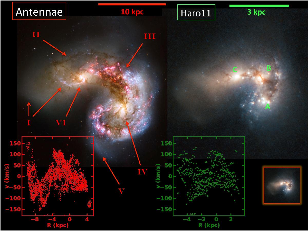
Antennae (left, credit STScI and B. Whitmore) and Haro 11 (right, Adamo et al. 2010, credit ESO/ESA/Hubble and NASA) put next to each other. The Antennae image has been rotated to the same apparent orientation as Haro 11 (which is shown as N up E left) and the images have been scaled so that the two systems look equally big on screen, for ease of comparison. The physical scale for the image of each system is shown with the red and green bars. In the image of Haro 11, we labelled the three main knots according to their common designation A, B, and C (Hayes et al. 2007). In the image of the Antenna we point out with arrows and roman numerals some regions of similarity, which are discussed in text. In the lower right inset we show the image of Haro 11 at the same physical scale of the Antennae. The image of Haro 11 is a composite of observations from HST/ACS (filters F435W, F550W, F814W) and VLT/NACO (K_s). The inset plot in red (lower left) show the position-velocity (PV) diagram for the Antennae (Amram et al. 1992) and the green inset to the right shows the same for Haro 11(this work). The PV diagrams have been extracted through the two nuclei in the Antennae and the corresponding for Haro 11 as seen in Fig. 9, i.e. knots and . Both PV diagrams cover the same total range in velocity (Δv = 250 km s^-1). The Antennae VF extend over 130′′ (16 kpc), while the one in Haro 11 covers 20′′ (8 kpc) and the same velocity scale. As is shown, the shape and amplitude of the PV diagrams are remarkably similar.