| Issue |
A&A
Volume 581, September 2015
|
|
|---|---|---|
| Article Number | A86 | |
| Number of page(s) | 11 | |
| Section | Cosmology (including clusters of galaxies) | |
| DOI | https://doi.org/10.1051/0004-6361/201526660 | |
| Published online | 09 September 2015 | |
The high-redshift gamma-ray burst GRB 140515A⋆,⋆⋆
A comprehensive X-ray and optical study
1
INAF–Osservatorio Astronomico Brera, via E. Bianchi 46, 23807 Merate ( LC),
Italy
e-mail:
This email address is being protected from spambots. You need JavaScript enabled to view it.
2
Instituto de Astrofísica de Andalucía (IAA-CSIC),
Glorieta de la Astronomía s/n,
18008
Granada,
Spain
3
Unidad Asociada Grupo Ciencias Planetarias (UPV/EHU, IAA-CSIC),
Departamento de Física Aplicada I, E.T.S. Ingeniería, Universidad del País Vasco
(UPV/EHU), Alameda de Urquijo
s/n, 48013
Bilbao,
Spain
4
Ikerbasque, Basque Foundation for Science, Alameda de Urquijo
36-5, 48008
Bilbao,
Spain
5
Universitá degli Studi dell’Insubria, via Valleggio 11, 22100
Como,
Italy
6
Racah Institute of Physics, The Hebrew University of
Jerusalem, 91904
Jerusalem,
Israel
7
Faculty of Mathematics and Physics, University of
Ljubljana, Jadranska ulica
19, 1000
Ljubljana,
Slovenia
8
Dark Cosmology Centre, Niels Bohr Institute, University of
Copenhagen, Juliane Maries Vej
30, 2100
Copenhagen,
Denmark
9
ASI – Science Data Center, via del Politecnico snc,
00133
Roma,
Italy
10 INAF–Osservatorio Astronomico di Roma, via Frascati 33,
00040 Monte Porzio Catone ( RM), Italy
11
The Oskar Klein Center, Department of Astronomy, AlbaNova,
Stockholm University, 10691
Stockholm,
Sweden
12
APC, U. Paris Diderot, CNRS/IN2P3, CEA/IRFU,
Obs. Paris, Sorbonne Paris Cité,
France
13
Particle Astrophysics Center, Fermi National Accelerator
Laboratory, Batavia,
IL
60510,
USA
14
Department of Astronomy & Astrophysics, The University
of Chicago, Chicago,
IL
60637,
USA
15
Kavli Institute for Cosmological Physics, The University of
Chicago, Chicago,
IL
60637,
USA
16
INAF – IASF Milano, via E. Bassini 15,
20133
Milano,
Italy
17
GEPI, Observatoire de Paris, CNRS, Univ. Paris Diderot, 5 place Jule Janssen,
92190
Meudon,
France
18
National Astronomical Observatories, Chinese Academy of
Sciences, 20A Datun Road, Chaoyang
District, 100012
Beijing, PR
China
Received: 2 June 2015
Accepted: 13 July 2015
Abstract
High-redshift gamma-ray bursts (GRBs) offer several advantages when studying the distant Universe, providing unique information about the structure and properties of the galaxies in which they exploded. Spectroscopic identification with large ground-based telescopes has improved our knowledge of this kind of distant events. We present the multi-wavelength analysis of the high-zSwift GRB GRB 140515A (z = 6.327). The best estimate of the neutral hydrogen fraction of the intergalactic medium towards the burst is xHI ≤ 0.002. The spectral absorption lines detected for this event are the weakest lines ever observed in GRB afterglows, suggesting that GRB 140515A exploded in a very low-density environment. Its circum-burst medium is characterised by an average extinction (AV ~ 0.1) that seems to be typical of z ≥ 6 events. The observed multi-band light curves are explained either with a very hard injected spectrum (p = 1.7) or with a multi-component emission (p = 2.1). In the second case a long-lasting central engine activity is needed in order to explain the late time X-ray emission. The possible origin of GRB 140515A in a Pop III (or in a Pop II star with a local environment enriched by Pop III) massive star is unlikely.
Key words: gamma-ray burst: general / gamma-ray burst: individual: GRB 140515A / galaxies: high-redshift / intergalactic medium
Based on observations collected at the European Southern Observatory, ESO, the VLT/Kueyen telescope, Paranal, Chile (proposal code: 093.A-0069), on observations made with the Nordic Optical Telescope, operated by the Nordic Optical Telescope Scientific Association at the Observatorio del Roque de los Muchachos, La Palma, Spain, of the Instituto de Astrofísica de Canarias (programme 49-008), and on observations made with the Italian 3.6-m Telescopio Nazionale Galileo (TNG), operated by the Fundación Galileo Galilei of the INAF (Instituto Nazionale di Astrofisica) at the Spanish Observatorio del Roque de los Muchachos, La Palma, Spain, of the Instituto de Astrofísica de Canarias (programme A26TAC_63).
Appendix A is available in electronic form at http://www.aanda.org
Deceased.
© ESO, 2015
1. Introduction
A better understanding of the chemical enrichment and evolution of the high-redshift Universe is one of the fundamental goals of modern astrophysics. High-redshift surveys have been performed by means of wide field surveys of bright quasars (e.g. Fan 2012) or deep field analyses to identify distant galaxies by how they drop-out (e.g. Bouwens et al. 2014). The identification of high-redshift gamma-ray bursts (GRBs) add a different and valuable view of the distant Universe (see Salvaterra 2015, for a recent review). With respect to other probes, GRBs have many advantages: (i) they are detected at higher redshifts; (ii) they are independent of the galaxy brightness; (iii) they do not suffer from usual biases affecting optical and/or near infrared (NIR) surveys; and (iv) they reside in average cosmic regions. High-z GRBs can provide fundamental and, in some cases, unique information about the early stages of structure formation and the properties of the galaxies in which they blow up. For example, GRBs can be used to trace the cosmic star formation rate (Kistler et al. 2009; Ishida et al. 2011; Robertson & Ellis 2012), to pinpoint high-z galaxies and explore their metal and dust content (Tanvir et al. 2009; Salvaterra et al. 2013; Elliott et al. 2015), to shed light on the re-ionisation history (Gallerani et al. 2008; McQuinn et al. 2008), to constrain both the dark matter particle mass (de Souza et al. 2013) and the amount of non-Gaussianity present in the primordial density field (Maio et al. 2012), and to measure the level of the local intergalactic radiation field (Inoue et al. 2010). Additionally, they can also provide direct and/or indirect evidence of the first massive, metal-free stars, the so-called Population III stars (Campisi et al. 2011; Toma et al. 2011; Wang et al. 2012; Ma et al. 2015).
Since the launch of the Swift satellite (Gehrels et al. 2004) seven events have been identified at redshift greater than 6, and for four of them spectroscopic redshift was secured, including in the list GRB 140515A that we discuss in this paper. Remarkably, some of them show fairly bright early afterglows, which are even detectable by small robotic telescopes (e.g. GRB 050904; Tagliaferri et al. 2005; Boër et al. 2006), but in general the observational features of high-z events do not seem to differ significantly from those of their closer siblings, as clearly seen when studying, for example, the event with the highest spectroscopically confirmed redshift, z ~ 8.2: GRB 090423 (Salvaterra et al. 2009; Tanvir et al. 2009).
In this paper we describe our observations of high-z GRB 140515A in Sect. 2 and the result of the analyses in Sect. 3. A discussion occurs in Sect. 4, and the main conclusions of our work are summarised in Sect. 5.
Throughout the paper, distances are computed assuming a Λ CDM-Universe with H0 = 71 km s-1 Mpc-1, Ωm = 0.27, and ΩΛ = 0.73 (Larson et al. 2011; Komatsu et al. 2011). Magnitudes are in the AB system and errors are at a 1σ confidence level. Raw and reduced data not explicitly reported in tables are available from the authors upon request.
2. Observations
On 2014 May 15 at 09:12:36 UT (=T0), the Swift/BAT triggered and located the long GRB 140515A (D’Avanzo et al. 2014). Swift/XRT promptly detected the afterglow emission whereas Swift/UVOT did not identify any credible bright optical candidate. A faint optical afterglow was later identified by ground-based observations with the 8 m Gemini-North telescope (Fong et al. 2014), the 2.5 m NOT telescope (de Ugarte Postigo et al. 2014a), the 2.2 m GROND telescope (Graham et al. 2014), and the 3.6 m TNG telescope (Melandri et al. 2014a).
Spectroscopic observations performed with the Gemini-North telescope (Chornock et al. 2014a) and the GTC telescope (de Ugarte Postigo et al. 2014b) detected sharp decrement in flux below 8900 Å, caused by Lyα absorption at redshift z = 6.327 (Chornock et al. 2014b). The spectral analysis is described in detail in Sect. 3.3.1.
3. Results
3.1. BAT temporal and spectral analysis
The Swift/BAT data were processed with the standard Swift analysis software included in NASA’s HEASARC software (HEASOFT, version 6.16) and the relevant latest calibration files. For each GRB, we extracted mask-weighted, background-subtracted light curves and spectra with the batmaskwtevt and batbinevt tasks in FTOOLS. The mask-weighted light curve shows a double-peaked structure. The first pulse started at T0−22 s and peaked at T0−18 s. It was followed by a second brighter pulse between T0−10 s and T0 + 4 s (see Fig. 1). The total duration of the burst event in the 15−150 keV energy band in the observer frame is T90 = (23.4 ± 2.1) s (90% confidence level), corresponding to ~3.2 s in the rest frame.
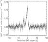 |
Fig. 1 BAT mask-weighted light curve showing the count rate in the 15−150 keV energy range. |
A fit to a simple power law of the time-averaged spectrum from T0−22 s to T0 + 4 s gives a photon index Γ = 1.86 ± 0.14 (χ2 = 61.21, d.o.f. = 56). A power law with an exponential cutoff gives a moderately better fit (χ2 = 54.57, d.o.f. = 55; F-test probability P = 98.8%). For this model the photon index is  ,
,  keV and the total fluence in the 15−150 keV band is
  erg/cm2. The 1 s peak flux measured from T0 + 1.50 s in the 15−150 keV band is fpk,BAT = 0.86 ± 0.10 ph cm-2 s-1.
We also tested for the presence of a blackbody component in the prompt emission spectrum. We added a blackbody component to the non-thermal (power-law) spectrum, and we fitted this model to the data, obtaining a photon index  and a blackbody temperature
  keV that, in the source rest frame, corresponds to
  keV. This model provides an adequate fit (χ2 = 54.29, d.o.f. = 54) but not a significant improvement over the cutoff power-law model.
We searched for a spectral evolution between the two main emission episodes of the prompt emission. The spectrum of the first peak (from T0−22 s to T0−14 s) can be modelled as a power-law spectrum with a photon index  . The spectrum’s second peak (from T0−14 s to T0 + 4 s) is represented better by a power law with an exponential cutoff (F-test probability P = 99.6%), with photon index
  ,
,  keV.
keV.
Assuming the exponential cutoff model, the total bolometric (rest frame 1−104 keV) isotropic energy is Eiso = (5.8 ± 0.6) × 1052 erg at z = 6.327 and  keV, consistent with the Epk,rf − Eiso correlation within its 1σ scatter (Amati 2006; Amati et al. 2008; Nava et al. 2012). The isotropic luminosity is Liso = (3.6 ± 0.8) × 1052 erg s-1, consistent with the Epk,rf − Liso correlation within its 1σ scatter (Yonetoku et al. 2004; Nava et al. 2012).
3.2. XRT temporal and spectral analysis
The XRT began observing ~60 s after the BAT trigger with the first 9 s in windowed timing (WT) mode and the remainder in photon counting (PC) mode. We collected the XRT data from the online Burst Analyzer (Evans et al. 2010) and converted the observed [0.3–10] keV count rate into flux at 3 keV. The X-ray light curve at that energy (Fig. 2) is described well by an initial steep decay (α1 ~ 2.9) followed by a broad bump after ~103 s that lasted for almost one day. From Fig. 1, it appears clear that the “real” burst began at T0,GRB = T0,real ~ T0−22 s. If we consider T0,GRB as the beginning of the burst, shifting the temporal axis of Fig. 2 backwards, the initial decay becomes less steep (α1 ~ 2.4), but it makes no difference for later breaks and decay indices (see Table 1).
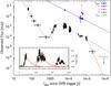 |
Fig. 2 Observed multi-wavelength light curve of GRB 140515A. We report the best fits for the optical (blue) and X-rays (grey) band. The orange line shows the possible decay of the late-time X-ray afterglow, assuming a possible jet break. Inset: the time interval of the X-ray bump on a linear scale. Red curves represent three independent flaring episodes. This is discussed further in Sect. 4.1 and Fig. 7. |
Observed X-ray light-curve fitting results (χ2/d.o.f. = 59.31/51 = 1.16 assuming that T0,GRB = T0, and χ2/d.o.f. = 55.89/51 = 1.09 if instead T0,GRB = T0,real).
Later on, a further steepening in the light curve is detected, also confirmed by Chandra’s deep upper limit. If we consider only XRT data, the late time decay index is αlate = 3.9 ± 0.6, while if we also take the deep late time upper limit into account, this value appears to be at least ≥2.6 (Margutti et al. 2014). Although it cannot be confirmed by the optical/NIR data, the late-time X-ray decay index might suggest a possible jet-break origin.
We performed a time-integrated spectral analysis of the X-ray emission from t − T0 = 86.4 s to t − T0 = 105 s using XSPEC version 12.8.2. The best fit to the data is an absorbed power law model: the Galactic absorption is kept fixed to the value  cm-2 (Willingale et al. 2013), the photon index is Γ = (1.79 ± 0.11) and the local absorption at z = 6.327 is NH< 5.6 × 1022 cm-2 (c-stat = 341.1, d.o.f. = 360). Selecting photons from t − T0 = 86.4 s to t − T0 = 2152 s, when the spectral changes are minor, we obtain an upper limit on the column density of NH< 8.9 × 1022 cm-2.
Also for the XRT spectrum we tested the presence of a possible blackbody component. The resulting fit, adding a thermal component to the power-law spectrum, did not improve the absorbed power law model described above.
The total isotropic energy in the 0.3−30 keV rest frame energy band is EX,iso = (7.19 ± 0.43) × 1051 erg, thus GRB 140515A is also consistent with the EX,iso − Epk,rf − Eiso correlation within its 2σ scatter (Bernardini et al. 2012; Margutti et al. 2013).
3.3. Optical/NIR temporal analysis
The Swift/UVOT began observing the field of GRB 140515A 3.7 ks after the trigger (D’Avanzo et al. 2014). The afterglow was not detected in any of seven UVOT filters. This is consistent with the redshift reported by Chornock et al. (2014a). To provide deep upper limits, we coadded the exposures within the first sequence of observations. We determined the count rate using a 5 arcsec circular source region centred on the optical afterglow position reported by Fong et al. (2014) and a circular background region of radius 20 arcsec positioned on a blank area of sky situated near the source position. The photometry was extracted using the UVOT tool uvotsource. The count rates were converted to magnitudes using the UVOT photometric zero points (Breeveld et al. 2011). We used Heasoft software version 6.15.1 and UVOT calibration version 20130118.
In Table 2 we summarise ultraviolet and optical 3σ upper limits and other optical/NIR detections of the optical afterglow. We note that at the redshift of GRB 140515A, the SDSS-z filter is slightly affected by the absorption of the intergalactic medium (IGM) since the optical depth for the Ly-α at z> 6 rises dramatically (i.e. Fan et al. 2006). Extrapolating the IGM properties from low redshift to z = 6.327 we estimated the expected correction for the z′ filter to be ≥0.30 mag (see Japelj et al. 2012 for details of the method). Even though this is formally a lower limit of the correction – not taking the rise in optical depth at z> 6 into account, we consider it before converting all the observed magnitudes reported in Table 2 into flux densities.
Optical observations.
Although the optical light curve is sparsely sampled (Fig. 2), it is possible to estimate the decay index of the optical afterglow in the z′-band at late times. From 6 ks after the burst event the optical afterglow follows a power-law decay with αz′ = 0.89 ± 0.02.
 |
Fig. 3 Flux-calibrated GTC spectrum: Lyα lines at z = 6.327 are shown in red, while the lines of the intervening system at z = 4.804 are shown in green. Black lines at the top of the panel mark telluric absorptions, with the thickness of the line indicating the absorption strength. At the bottom the error spectrum is shown (blue), while the parts of the spectrum where the strength of the sky emission lines is strong enough to leave significant residuals have been masked with light blue columns. The spectrum has been smoothed with a Gaussian filter. |
3.4. Optical/NIR spectral analysis
3.4.1. GTC spectrum
We obtained spectroscopy of the afterglow of GRB 140515A with OSIRIS (Cepa et al. 2000) at the 10.4 m Gran Telescopio Canarias (de Ugarte Postigo et al. 2014b). The observations were obtained between 22:37:31 UT and 00:09:46 UT (mean epoch 14.184 h after the GRB onset) with 0.6′′ seeing, and they consisted of 3 × 1800 s exposures. We used the R2500I VPH grism, which covers the range between 7330 and 10 000 Å at a resolution of ~1600 using a 1′′ slit.
The data were reduced in a standard way (bias subtraction, pixel-to-pixel response correction, cosmic ray removal, wavelength calibration, 1D extraction, flux calibration, and combination of spectra) using self-made routines based on IRAF (Tody 1993). The resulting combined GTC spectrum (Fig. 3) shows a strong continuum above ~8900 Å, where the signal-to-noise ratio is ~20 per pixel, or ~40 per resolution element.
3.4.2. X-Shooter spectrum
We observed the field of GRB 140515A with the X-Shooter spectrograph mounted at the ESO/VLT using the nodding mode with 1 × 2 binning. The spectrum was acquired on 2014 May 16, starting at 00:42:43 UT (~15.5 h after the GRB onset), and consisted of 2 × 4 × 600 s exposures, for a total integration time of 4800 s on source, covering the range between ~3000 and ~24 000 Å. The mid exposure time is 16.3 h (~0.68 d) after the GRB trigger. The final reduced spectrum (see Fig. A.1) has a signal-to-noise ratio (S/N) of ~3 per pixel1, with a seeing of ~0.9′′ (measured from combined 2D spectrum in the VIS and NIR arms). The flux calibration of the X-Shooter, which is problematic in general (Krühler et al. 2015; Japelj et al. 2015), is uncertain due to unavailable standard spectrophotometric stars in the night when the observations were done and because the photometric observations, which could be used to check the quality of calibration, had rather high errors at this epoch. Thus, it is not possible to use them to reliably rescale the spectrum.
3.4.3. Lyα forest constraints on the IGM
We analysed the ionisation state of the IGM using the Gunn & Peterson (1965) optical depth, defined as  , where
  is the average transmission in a redshift bin. Following Songaila & Cowie (2002) and Songaila (2004), we normalised the GTC spectrum (as its S/N is better than the X-Shooter one, see Sect. 3.4.4) by fitting a power law to the continuum, and divided it into redshift bins of 0.1 between z = 5.2 and z = 6.3. The results are presented in Fig. 4 and in Table 3.
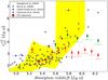 |
Fig. 4 Lyα effective optical depth in the line of sight of GRB 140515A compared with previous GRB and QSO works. The coloured area shows the optical depth found by Songaila (2004), while grey points are measurements from Fan et al. (2006) with a sample of quasars. |
IGM absorption towards GRB 140515A.
We only see sky line residuals up to z ~ 5.5, above which we can just give detection limits based on the noise spectrum. Our limits are less restrictive than the ones presented by Chornock et al. (2014b) owing to the lower S/R, but show the same behaviour (Fig. 4). Results coming from both GRB 140515A and GRB 130606A (Chornock et al. 2013; Castro-Tirado et al. 2015; Hartoog et al. 2015) are consistent with quasar measurements (Songaila 2004; Fan et al. 2006).
3.4.4. Lyα red-damping wing fitting
We tried to fit the strongest feature seen in the spectrum (at ~8900Å) to an absorption Lyman-α feature with a Voigt profile. Following Chornock et al. (2014b), we first computed a Voigt model using the same constraints, obtaining inconsistent results. This could be because they do not seem to consider the instrumental profile, the effect of which on the Ly-α feature is not negligible at this resolution when log (NHI) ≲ 19. Looking at Fig. 5, we can observe the residuals of a sky line subtraction that is a few angstroms blue-wards of the wing, precisely at the zone crucial to fit a Voigt model. After a careful inspection of the 2D images of both GTC and X-Shooter instruments, we concluded that there is no flux in this zone. Consequently, the wing profile is too sharp to get a satisfactory fit, suggesting that the absorption is dominated by the IGM and that the host absorption is masked.
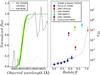 |
Fig. 5 Left: best IGM damping wing fit to the spectrum of GRB 140515A. Right: redshift evolution of the hydrogen neutral fraction. The dotted line shows the Gnedin & Kaurov (2014) model and points to (see legend) the observational measurements of this quantity (data from Totani et al. 2006; Patel et al. 2010; and Chornock et al. 2013). Points with arrows are lower or upper limits. |
We then built our IGM models following the prescription of Miralda-Escudé (1998), fixing the lower redshift value to z = 6.0 because the contribution to the wing shape below this redshift is negligible. It starts to be important closer to the host. Our best fit, with z = 6.3298 ± 0.0004 and a fraction of neutral hydrogen xHI ≤ 0.002, is shown in Fig. 5. We caution that, due to the sharpness of the wing, the few points we have because of GTC resolution and the sky line next to the absorption, any formal constraints on these quantities would be unreliable. This means the values should be interpreted as the most plausible estimations that we can obtain from the data. Moreover, especially because z cannot be determined by metal lines, hybrid models cannot offer a more accurate fit than the one showed in Fig. 5, so no constraints on the host HI abundance can be derived from this event (for further discussion, see Miralda-Escudé 1998). However, due to the sharpness of the red damping wing, it is obvious that the neutral hydrogen present in the IGM cannot mask either the presence of a DLA nor a sub-DLA, because their damping wings would be easily identified. Consequently, we can establish a conservative upper limit of log (NHI) ≲ 18.5 for the HI abundance in the host galaxy of GRB 140515A. As shown in Fig. 5, the fraction of neutral hydrogen derived from this analysis fits well with the model by Gnedin & Kaurov (2014), and it provides a very relevant observational constraint.
Last of all, we estimated the 3σ upper limits on the observer-frame equivalent width (EW) for the Si II λ1260, O I λ1302, and C II λ1334 lines. We find a value of 0.67 Å, 1.06 Å, and 1.30 Å, respectively. These estimates are a factor ~2 more stringent than those reported by Chornock et al. (2014b), resulting in upper limits on the gas-phase abundances of [ Si / H ] ≲ −1.4, [ O / H ] ≲ −1.1, and [ C / H ] ≲ −1.0. Furthermore, these lines are weaker than the average rest-frame EWs observed for a typical GRB (de Ugarte Postigo et al. 2012). In fact, the strength of those lines compared to the average GRB spectrum that can be estimated with the use of the line strength parameter (LSP, as defined in de Ugarte Postigo et al. 2012), is LSP < –3.15, <–3.89, and <–2.88, respectively. This means that these lines are very weak and that GRB 140515A exploded in a relatively low-density environment. However, our limits on the metals abundances do not allow us to put a stringent limit on the metallicity of the progenitor.
3.4.5. Spectral energy distribution
We constructed a broadband spectral energy distribution (SED) using the flux-calibrated X-Shooter spectrum and Swift X-ray data (Fig. 6). X-Shooter data are treated as outlined in Japelj et al. (2015). The spectrum was corrected for Galactic extinction (E(B − V) = 0.02 mag) by using the Cardelli et al. (1989) extinction curve and Galactic extinction maps (Schlafly & Finkbeiner 2011). Regions of telluric absorption were masked out. The spectrum was re-binned in bins of approximately 50 Å to increase S/N and to guarantee a comparable weight of the optical and X-ray SED part. The absolute flux calibration was fine-tuned with simultaneously obtained near-infrared photometric observations. The X-ray part of the SED was built from time-integrated observations obtained between 5–60 ks and its mean epoch was interpolated to the mean epoch of the X-Shooter observations.
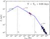 |
Fig. 6 Spectral energy distribution (solid line) obtained with X-Shooter (red) and XRT data (black), corrected for the rest-frame AV and NH respectively. We also included the radio detection (green) of Laskar et al. (2014). The dashed blue line represents the extinction uncorrected best-fit. Dashed lines indicate the position of the injection frequency (νi = 2 × 10¹² Hz) and the cooling frequency (νc ~ 2 × 10¹⁶ Hz) expected for a pure synchrotron model. |
The SED fitting was carried out with the spectral fitting package XSPECv12.8 (Arnaud 1996). We model the SED with either a single or broken power-law intrinsic spectrum. For the latter we assume βX = βO + 0.5 (Sari, et al. 1998). Extinction is modelled with the three commonly assumed extinction curves to be found in Milky Way, Large and Small Magellanic Cloud (Pei 1992). Only the spectrum red-wards of Lyα line has been used in the analysis. The broadband SED is best described by a broken power law and an SMC-type extinction with AV = 0.11 ± 0.02 mag and βO = 0.33 ± 0.02. By requiring Δβ = 0.5, it has been possible to better constrain the X-ray column density to  cm-2. This value is consistent with the direct estimate from X-ray data alone (see Sect. 3.2). In the absence of a very good SED, it is feasible and justified to use a generic SMC extinction curve to model our data. At such a high-z, our wavelength range is very narrow and so is difficult to separate between different extinction curves even though, in principle, the dust properties may differ, as already suggested by several examples (e.g. Perley et al. 2008; Fynbo et al. 2014; Friis et al. 2015).
As a consistency check we also built the spectral energy distribution of the optical afterglow using all the available photometric observations reported in Table 2 and in the Swift X-ray data. The extinction estimated with photometric information (AV ~ 0.6 mag) is much higher than the one obtained from the more accurate spectral analysis reported above. This is because photometric measurements are too sparse to give reliable results. The rest-frame extinction (AV ~ 0.1 mag) of GRB 140515A is consistent with the AV distribution found for the complete BAT6 sample (Covino et al. 2013), and suggests that this is also a typical value for high-z events.
4. Discussion
4.1. Late time flare emission/refreshed shock
The most straightforward explanation for the observed X-ray peak at t ~ 3000 s (Fig. 2) is the onset of the afterglow emission. This interpretation is supported by the rise and decay indices of the X-ray light curve, which are consistent with the expectations for the emission of the forward shock interacting with a homogeneous medium. An alternative possibility is that the X-ray peak corresponds to a late-time flaring activity or to variability of the GRB afterglow interacting with the ambient medium. A powerful tool for investigating the nature of this variability is the comparison of the flux increase as a function of the temporal variability of the peak with the regions of allowance for bumps in the afterglow on the basis of kinematic arguments (Ioka et al. 2005). This diagnostic tool has been successfully applied to GRBs displaying early- and/or late-time strong variability (e.g. Margutti et al. 2010; De Cia et al. 2011; Melandri et al. 2014b). In Fig. 7 we portrayed the sample of early-time (tpk ≲ 1 ks) flares (Chincarini et al. 2010) and late-time (tpk ≳ 1 ks) flares (Bernardini et al. 2011).
If we interpret the broad X-ray bump of GRB 140515A as a single long-lasting flaring episode it would occupy a different region with respect to the observed X-ray flares since it is characterised by a very long duration (Δt/tpk ~ 50 ≫ 1) and large flux variation (Δf/f ~ 102). It would therefore be consistent with being produced by refreshed shocks (Rees & Mészáros 1998; Kumar & Piran 2000b; Sari & Mészáros 2000), or with an intrinsic angular structure on the emitting surface (a “patchy shell”) (Mészáros et al. 1998; Kumar & Piran 2000a), or by shock reflection generated by the interaction of the reverse shock with dense shells formed at an earlier stage of the explosion (Hascoët et al. 2015). An increase in the external medium density (e.g. Jakobsson et al. 2004) would require a sharp and large jump in a uniform density profile to produce the observed increase in the observed light curves, which seems unlikely.
A single X-ray broad peak is well outside the region of validity for the internal shock model. However, there is still the possibility that the broad single peak that we observe is the result of the superposition of multiple peaks, each with Δt/tpk ≪ 1. In the inset of Fig. 2 we sketched a possible temporal behaviour for GRB 140515A, where three flaring events (with a typical profile as described in Norris et al. 2005), superimposed to the underlying temporal decay, could be responsible of the shape of the broad bump observed. If we consider this scenario the observed behaviour becomes consistent with the internal shocks scenario (Fig. 7). This situation resembles the case of GRB 050904, a GRB at very similar redshift (z = 6.29) that shows a late time variability in the X-rays and a sudden drop of the observed emission afterwards. However, GRB 140515A is fainter than GRB 050904, and its variability has not been fully captured by the XRT.
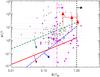 |
Fig. 7 Kinematically allowed regions for afterglow variability in the Δf/f vs. Δt/tpk plane. Coloured lines with arrows represent the permitted regions for density fluctuations on-axis (blue), density fluctuations off-axis (red), multiple density fluctuations off-axis (green), refreshed shocks (pink), and patchy shell (black). (See Ioka et al. 2005; Chincarini et al. 2010; Bernardini et al. 2011, for details.) In this plot we show early-time (tpk ≲ 1 ks, grey points) and late-time (tpk ≳ 1 ks, magenta squares) flares. The red triangles are the three flaring episodes in GRB 140515A. The error bars account for the uncertainty on the behaviour of the underlying continuum: the lower bar corresponds to a flat power-law decay after 103 s, the high bar to a flat decay normalised to the last datapoint, and the central value to a power-law decay consistent with the slope of the optical light curve after 103 s. |
4.2. Standard afterglow interpretation
To explain the observed light curves, we consider a semi-analytic model that describes the dynamical evolution of the fireball when interacting with the external circumburst medium and the respective radiative emission in the standard forward shock scenario (Nava et al. 2013). The radiative description is based on the model illustrated by Nappo et al. (2014), which allows us to compute the synchrotron spectrum as a function of time, normalised to the bolometric luminosity obtained by the dynamical model. We assume that the electrons are injected with a power – law energetic distribution with index p and can cool for synchrotron and synchrotron self-Compton (SSC) radiation. The model allows us to obtain at each step:
-
(i)
the synchrotron break frequencies (i.e. the self-absorptionfrequency νa, the injection frequency νi, and the cooling frequency νc);
-
(ii)
the fraction of dissipated energy that is emitted in radiation ϵrad that is used to determine the bolometric luminosity;
-
(iii)
the comptonisation parameter Y;
-
(iv)
the synchrotron spectrum Lν,syn.
Since the spectrum of the radiation is estimated each time, the light curve at a specific frequency Fν(tobs) can be derived.
The parameters that can be varied to reproduce the observed light curves are the initial bulk Lorentz factor (Γ0), the isotropic prompt emitted energy Eiso, the prompt radiation efficiency (η), the circumburst density (n, in case of homogeneous medium), the injected electron spectral index (p), and the fraction of dissipated energy distributed to the leptons (ϵe) and to the magnetic field (ϵB). The model assumes an isotropic ejecta so it cannot reproduce geometrical features, such as jet break and side-expansion effects.
From the modelling, two different interpretations of the multi-wavelength light curve of GRB 140515A are possible: a pure synchrotron emission by electrons with a very hard spectrum (with p< 2) or a multi-component model (with p> 2). We considered only the radio, J, H, and the X-ray band emissions, since, as shown in Sect. 3.3, the optical SDSS-z′ emission is strongly affected by absorption, and the resulting flux is very likely underestimated.
4.2.1. A very hard injected spectrum
We model the observations in the J, H, radio, and X-ray bands as synchrotron radiation produced in the forward shock. To obtain a successful modelling, we need to assume that the electron injection spectrum is a power law with a very hard index (p = 1.67) that extends up to the maximum Lorentz factor γmax. Even in this case, the model cannot find a solution for the early time (very steep) X-ray emission. As suggested by Ghisellini et al. (2009) among others, we assume that the X-ray light curve is composed of a late prompt component decaying with time as a power law of slope ≥–3 (dominant for tobs ≲ 600 s) and by a second component interpreted as the actual X-ray afterglow emission (tobs ≳ 600 s).
A good description of the detection in J, H, radio, and X-ray bands (Fig. 8, dashed lines) was obtained using the parameters reported in Table 4. The bump observed in the X-ray light curve is due to the onset of the afterglow, which correspond to Γ0 = 195.
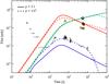 |
Fig. 8 Two multi-wavelength interpretations of the GRB 140515A afterglow light curve in X-ray band (black dots, blue lines), SDSS-z′ band (yellow circles), J band (orange circles), H band (red circles, red lines) and radio band (green star, green lines). Dashed lines represent the solution in the “hard electron spectrum” scenario (p = 1.67). Solid lines describe the solution for the “multi-component” scenario (p = 2.1). |
Parameters of the proposed light curve scenarios.
The last detection in the X-ray band shows a sudden drop in the X-ray flux. The temporal index after the break is very steep (αlate = 3.9 ± 0.6, see Table 1) and is not consistent with theoretical predictions from jetted outflows. As an alternative we then suggest that this steepening is due to the passage of the maximum synchrotron frequency (associated to the maximum Lorentz factor γmax of the electrons) in the X-ray band. To model the maximum frequency, we assume that the ratio between the maximum and minimum Lorentz factors of the electrons is constant in time, and is equal to γmax/γmin ≃ 2800. This interpretation allows us to describe the observations fully with no need for a jet break. Since the light curve does not show any break until 105s, this time represents a lower limit on the jet break time. The corresponding lower limits on the jet opening angle and on the collimation corrected energy Eγ are reported in Table 4. This lower limit on Eγ is consistent with the Epk − Eγ correlation (Ghirlanda et al. 2004). Consistency with this correlation, in fact, requires a jet break at times greater than 3.5 × 10⁵s, strengthening the hypothesis that the steep break in the late X-ray light curve is not due to the jetted geometry of the outflow.
4.2.2. Multi-component model
An alternative interpretation could be obtained with a steeper electron injected spectrum. However, in this case it is not possible to obtain a pure synchrotron solution that can correctly explain the J, H, the X-ray emission and the radio detection. In fact, if we describe simultaneously the J, H and radio emissions, we underestimate the X-ray light-curve. As also shown in previous sections, the peculiar shape of the X-ray light curve, characterised by an important time variability up to tobs ~ 104 s, suggests that the X-ray emission at those times could probably be caused by the composition of the standard afterglow emission in a forward shock scenario and some additional emissions (for instance, flares, or a long-lasting prompt emission).
Therefore, the time of the X-ray peak must be similar to the deceleration time computed by the model. Moreover, the predicted X-ray emission cannot overcome the observed flux, since it must be a composition of the afterglow and additional emissions. In this scenario, we expect the rise in the X-ray flux (at tobs ~ 103 s) to correspond to the rise in the X-ray afterglow. Adding few constraints, we obtain a compatible multi-wavelength prediction of the afterglow light curve (see solid lines in Fig. 8). The set of parameters for this scenario is reported in Table 4.
In this scenario the X-ray afterglow prediction is below the observed data at early-times, while the last observed detection becomes compatible with the expected afterglow emission. This is consistent with the hypothesis of a multi-component X-ray emission, and we can assume that it is only for tobs ≳ 2 × 10⁵ s that we observe a pure X-ray afterglow emission that is not contaminated by long-lasting central engine activity.
At the time of the Chandra observation, the X-ray afterglow flux predicted by this modelling is marginally consistent with the Chandra upper limit. A jet break around this time would make the energetics consistent with the prediction of the Epk − Eγ correlation. However, since a break is not strictly required by our modelling, we have set a conservative lower limit on the jet break at tjet> 2 × 10⁵s. The corresponding lower limits on the jet opening angle and on the collimation corrected energy are listed in Table 4.
4.3. Pop III or enriched Pop II progenitor
GRB 140515A shows evidence of long-lasting central-engine activity up to ~104 s after the burst event. Its redshift (z> 6) could suggest a Pop III star progenitor. These types of massive stars (M ≥ 100 M⊙), which are thought to form in the early Universe at low metallicity (Z ~ 10-4Z⊙), have also been proposed as progenitor of the so-called ultra-long GRBs (Salvaterra et al. 2013; Ma et al. 2015), i.e. GRB 111209A (Gendre et al. 2013), GRB 121027A (Hou et al. 2014), and GRB 130925A (Evans et al. 2014).
In this scenario, the long duration is the result of the time needed for the accretion and collapse mechanisms. In the hypothesis of such a GRB progenitor, one would expect to detect a very low-density environment with a density profile dominated by the IGM. Another expectation for such massive collapsing stars is a long-lasting blackbody emission component in their spectra, with a typical average rest-frame temperature of kTBB ~ 0.5 keV (Piro et al. 2014). This thermal emission would, in principle, be detectable by BAT and/or XRT if the redshift of the event is low.
In the case of GRB 140515A, our observations support the idea of a low density environment with negligible contribution from the host galaxy but there are no hints of a particularly low value in the metallicity (see Sect. 3.4.3). Moreover, being at such a high-z we did not detect any blackbody component with Swift instruments (see Sect. 3.1), and we did not find any improvement of the fit with the inclusion of a blackbody component in the prompt emission spectrum. Therefore, the hypothesis that GRB 140515A originated in a Pop III star (or even in a Pop II star with environment enriched by Pop III stars) is unlikely.
4.4. Reionization and escape fraction of ionizing radiation
The distribution of intrinsic column densities of GRB hosts can be used to constrain the average escape fraction of ionizing radiation from the hosts (Chen et al. 2007), based on the assumption that GRB sight lines, taken as an ensemble, sample random lines of sight from star forming regions in GRB hosts. At intermediate redshifts (z> 2), the sample of GRB hosts from Chen et al. (2007) indicates that only in about 5% of all cases does one expect a GRB sightline with log (NHI) < 18.5. With GRB 140515A being only one out of seven GRBs with z> 6 (and only one out of three with measured HI column densities), it appears that high-redshift GRB hosts may have, on average, lower HI column densities, hence higher escape fractions than their lower redshift counterparts.
More quantitatively, the Kolmogorov-Smirnov test for the two distributions of HI column densities – first from Chen et al. (2007) and the second of four z> 5.9 GRBs with measured NHI values – shows that the two distributions are consistent with only 9% probability. That probability rises to 30% if GRB 140515A is excluded. The importance of constraining the escape fractions in reionisation sources is obvious, so a larger sample of z> 6 GRBs with measured HI column densities would be highly desirable.
Such a sample would also serve as a direct test of reionisation at z> 6, where constraints from high redshift quasars become scarce. A significant advantage of GRBs over quasars is in their low or negligible bias. While bright quasars often do reside in the most massive, highly biased dark matter halos, GRB hosts at high-z seem to sample the general galaxy population. As a result, constraints for the neutral hydrogen fraction obtained from the analysis of the IGM damping wing profile in the absorption spectra of GRB hosts can be expected to be more reliable than the analogous constraints from the quasar proximity zones.
In addition, constraints on the mean neutral fraction from observations of QSO proximity zones are, typically, lower limits (neutral fraction can be larger if a quasar lifetime is longer) (Bolton et al. 2011; Robertson et al. 2013, 2015), while constraints from GRBs are upper limits. The two observational probes are therefore highly complementary to each other (demonstrated by red and orange diamonds in Fig. 5).
Absorption properties of the GRBs with z ≥ 5.
4.5. High-z GRBs absorption properties
In Table 5 we report the absorption properties – neutral hydrogen column density in the host galaxy (NHI), X-ray equivalent column density (NH,X), and optical dust extinction (AV) – for all known GRBs with redshift z ≥ 5. As shown in Table 5, host galaxies of high-z GRBs have low but not zero extinction, and the value of their optical extinction remains, in fact, rather constant (0.1 ≲ AV ≲ 0.2 mag) over a broad range of redshifts.
It should be noted that no high values for AV have ever been detected for GRBs at redshift ≥5, and this is probably due to an observational bias, since it would be difficult to carry out optical follow-ups. Nevertheless, owing to the general low level of metal abundances of the young galaxies at such high z, it is also plausible that high extinctions are intrinsically less probable than at lower redshifts.
While the AV does not seem to evolve with redshift, there are no detected events with low NH,X at z ≥ 6. This effect can be explained naturally by the increase in absorption of the intervening systems along the line of sight (Campana et al. 2012; Covino et al. 2013; Campana et al. 2015; Salvaterra 2015). This mimics the evolution of the NH/AV ratio with redshift observed in Fig. 9 (bottom panel) up to z ~ 10.
 |
Fig. 9 AV, NH, and NH/AV ratio as a function of redshift. Black points are from Covino et al. (2013) for events with z ≲ 4, while the remaining events (blue circles, purple stars) are listed in Table 5. GRB 140515A is marked with a red star. The solid and/or dashed gray lines in the middle panel represent the effect of the intervening material along the line of sight (see Campana et al. 2015; Salvaterra 2015). |
5. Conclusion
We have presented the multi-band spectroscopic and temporal analysis of the high-z GRB 140515A. The overall observed temporal properties of this burst, including the broad X-ray bump detected at late times, could be explained in the context of a standard afterglow model, although this requires an unusually hard index of the electron energy spectrum (p = 1.67). Another possible interpretation is to assume that an additional component (e.g. related to long-lasting central engine activity) is dominating the X-ray emission. In that case, the broadband observations can be explained using a more typical value of the spectral index for the injected electron spectrum (p = 2.1). Our modelling in this case shows that the central engine activity should cease at late times (~2 × 10⁵s), when the X-ray afterglow starts to dominate the emission. In both scenarios the cooling frequency is expected to be between the optical and the X-ray energy bands (νc ~ 2 × 10¹⁶ Hz), and the average rest-frame circumburst extinction (AV ~ 0.1) turned out to be typical of high-z bursts.
Our detailed spectral analysis provided a best estimate of the neutral hydrogen fraction of the IGM towards the burst of xHI ≤ 0.002 and a conservative upper limit of the HI abundance in the GRB host galaxy of NHI ≲ 1018.5 cm-2. These values are slightly different from the ones estimated by Chornock et al. (2014b). In addition, the spectral absorption lines observed in our spectra are the weakest lines ever observed in GRB afterglows (de Ugarte Postigo et al. 2012), suggesting that GRB 140515A happened in a very low-density environment. However, our upper limits on the gas-phase abundances, coupled with the fact that we cannot establish the exact metal-to-dust ratio, do not allow us to distinguish between metallicity in the range of 10-4< [ Z / H ] < 0.1. This makes the possible Pop III star origin for GRB 140515A uncertain and doubtful.
For all high-z GRBs, the contribution of the host galaxy was not negligible (Table 5). GRB 140515A is the first case where this does not happen, allowing us to give the best observational constraints on a theoretical model at z> 6.
Online material
Appendix A: X-Shooter spectrum
 |
Fig. A.1 X-Shooter spectrum: Lyα lines at z = 6.327 are indicated in red, while the lines of the intervening system at z = 4.804 are marked in green. Black lines at the top of the panel mark telluric absorptions, with the thickness of the line indicating the absorption strength. At the bottom the error spectrum is shown (blue). The spectrum has been smoothed with a Gaussian filter. |
The quoted difference in S/N between the GTC and X-Shooter spectra is due partly to the different pixel size of the two instruments and partly to the better observing conditions of the GTC observation.
Acknowledgments
We thank the anonymous referee for the valuable comments that contributed to improving the quality of the publication. This research has been supported by ASI grant INAF I/004/11/1. D.M. acknowledges support from the Instrument Center for Danish Astrophysics (IDA). The Dark Cosmology Centre is funded by the Danish National Research Foundation. This work made use of data supplied by the UK Swift Science Data Centre at the University of Leicester.
References
- Amati, L. 2006, MNRAS, 372, 233 [NASA ADS] [CrossRef] [Google Scholar]
- Amati, L., Guidorzi, C., Frontera, F., et al. 2008, MNRAS, 391, 577 [NASA ADS] [CrossRef] [MathSciNet] [Google Scholar]
- Arnaud, K. A. 1996, ASP Conf. Ser., 101, 17 [Google Scholar]
- Bernardini, M. G., Margutti, R., Chincarini, G., et al. 2011, A&A, 526, A27 [NASA ADS] [CrossRef] [EDP Sciences] [Google Scholar]
- Bernardini, M. G., Margutti, R., Zaninoni, E., & Chincarini, G. 2012, MNRAS, 425, 1199 [NASA ADS] [CrossRef] [Google Scholar]
- Boër, M., Atteia, J. L., Damerdji, Y., et al. 2006, ApJ, 638, 71 [Google Scholar]
- Bolton, J. S., Haehnelt, M. G., Warren, S. J., et al. 2011, MNRAS, 416, 70 [NASA ADS] [CrossRef] [Google Scholar]
- Bouwens, R. J., Illingworth, G. D., Oesch, P. A., et al. 2014, ApJ, 793, 115 [Google Scholar]
- Breeveld, A. A., Landsman, W., Holland, S. T., et al. 2011, AIP Conf. Ser., 1358, 373 [Google Scholar]
- Campana, S., Salvaterra, R., Melandri, A., et al. 2012, MNRAS, 421, 1697 [NASA ADS] [CrossRef] [Google Scholar]
- Campana, S., Salvaterra, R., Ferrara, A., & Pallottini, A. 2015, A&A, 575, A43 [NASA ADS] [CrossRef] [EDP Sciences] [Google Scholar]
- Campisi, M. A., Maio, U., Salvaterra, R., & Ciardi, B. 2011, MNRAS, 416, 2760 [NASA ADS] [CrossRef] [Google Scholar]
- Cardelli, J. A., Clayton, G. C., & Mathis, J. S. 1989, ApJ, 345, 245 [NASA ADS] [CrossRef] [Google Scholar]
- Castro-Tirado, A. J., Sánchez-Ramírez, R., Ellison, S. L., et al. 2015, ArXiv e-prints [arXiv:1312.5631] [Google Scholar]
- Cepa, J., Aguiar, M., Escalera, V. G., et al. 2000, SPIE, 4008, 623 [Google Scholar]
- Chen, H.-W., Prochaska, J. X., & Gnedin, N. Y. 2007, ApJ, 667, L125 [NASA ADS] [CrossRef] [Google Scholar]
- Chincarini, G., Mao, J., Margutti, R., et al. 2010, MNRAS, 406, 2113 [NASA ADS] [CrossRef] [Google Scholar]
- Chornock, R., Berger, E., Fox, D. B., et al. 2013, ApJ, 774, 26 [NASA ADS] [CrossRef] [Google Scholar]
- Chornock, R., Fox, D. B., & Berger, E. 2014a, GRB Coord. Network, 16269, 1 [Google Scholar]
- Chornock, R., Berger, E., Fox, D. B., et al. 2014b, ArXiv e-prints [arXiv:1405.7400] [Google Scholar]
- Covino, S., Melandri, A., Salvaterra, R., et al. 2013, MNRAS, 432, 1231 [NASA ADS] [CrossRef] [Google Scholar]
- D’Avanzo, P., Bernardini, M. G., D’Elia, V., et al. 2014, GRB Coord. Network, 16267, 1 [Google Scholar]
- De Cia, A., Jakobsson, P., Björnsson, G., et al. 2011, MNRAS, 412, 2229 [NASA ADS] [CrossRef] [Google Scholar]
- de Ugarte Postigo, A., Fynbo, J. P. U., Thöne, C. C., et al. 2012, A&A, 548, A11 [NASA ADS] [CrossRef] [EDP Sciences] [Google Scholar]
- de Ugarte Postigo, A., Gorosabel, J., Xu, D., et al. 2014a, GRB Coord. Network, 16278, 1 [Google Scholar]
- de Ugarte Postigo, A., Gorosabel, J., Thoene, C. C., et al. 2014b, GRB Coord. Network, 16279, 1 [Google Scholar]
- de Souza, R. S., Mesinger, A., Ferrara, et al. 2013, MNRAS, 432, 3218 [NASA ADS] [CrossRef] [Google Scholar]
- Elliott, J., Khochfar, S., Greiner, J., & Dal la Vecchia, C. 2015, MNRAS, 446, 4239 [NASA ADS] [CrossRef] [Google Scholar]
- Evans, P., Willingale, R., Osborne, J. P., et al. 2010, A&A, 519, A102 [NASA ADS] [CrossRef] [EDP Sciences] [Google Scholar]
- Evans, P. A., Willingale, R., Osborne, J. P., et al. 2014, MNRAS, 444, 250 [NASA ADS] [CrossRef] [Google Scholar]
- Fan, X. 2012, Res. Astron. Astrophys., 12, 685 [Google Scholar]
- Fan, X., Strauss, M. A., Becker, R. H., et al. 2006, AJ, 132, 117 [NASA ADS] [CrossRef] [EDP Sciences] [Google Scholar]
- Fong, W., Chornock, R., Fox, D., & Berger, E. 2014, GRB Coord. Network, 16274, 1 [Google Scholar]
- Friis, M., De Cia, A., Krühler, T., et al. 2015, MNRAS, 451, 4686 [Google Scholar]
- Fynbo, J. P. U., Krühler, T., Leighly, K., et al. 2014, A&A, 572, A12 [NASA ADS] [CrossRef] [EDP Sciences] [Google Scholar]
- Gallerani, S., Salvaterra, R., Ferrara, A., & Choudhury, T. R. 2008, MNRAS, 388, L84 [NASA ADS] [Google Scholar]
- Gehrels, N., Chincarini, G., Giommi, P., et al. 2004, ApJ, 611, 1005 [NASA ADS] [CrossRef] [Google Scholar]
- Gendre, B., Stratta, G., Atteia, J. L., et al. 2013, ApJ, 766, 30 [NASA ADS] [CrossRef] [Google Scholar]
- Ghirlanda, G., Ghisellini, G., & Lazzati, D. 2004, ApJ, 616, 331 [NASA ADS] [CrossRef] [Google Scholar]
- Ghisellini, G., Nardini, M., Ghirlanda, G., & Celotti, A., 2009, MNRAS, 393, 253 [NASA ADS] [CrossRef] [Google Scholar]
- Gnedin, N. Y., & Kaurov, A. A. 2014, ApJ, 793, 30 [NASA ADS] [CrossRef] [Google Scholar]
- Graham, J., Schmidl, S., Greiner, J. 2014, GRB Coord. Network, 16280, 1 [Google Scholar]
- Gunn, J. E., & Peterson, B. A. 1965, ApJ, 142, 1633 [NASA ADS] [CrossRef] [Google Scholar]
- Hartoog, O. E., Malesani, D., Fynbo, J. P. U., et al. 2015, A&A, 580, A139 [NASA ADS] [CrossRef] [EDP Sciences] [Google Scholar]
- Hascoët, R., Beloborodov, A. M., Daigne, F., & Mochkovitch, R. 2015, MNRAS, submitted [arXiv:1503.08333] [Google Scholar]
- Hou, S.-J., Gao, H., Liu, T., et al. 2014, MNRAS, 441, 2375 [NASA ADS] [CrossRef] [Google Scholar]
- Inoue, S., Salvaterra, R., Choudhury, T. R., et al. 2010, MNRAS, 404, 1938 [NASA ADS] [Google Scholar]
- Ioka, K., Kobayashi, S., & Zhang, B. 2005, ApJ, 631, 429 [NASA ADS] [CrossRef] [Google Scholar]
- Ishida, E. E. O., de Souza, R. S., & Ferrara, A. 2011, MNRAS, 418, 500 [NASA ADS] [CrossRef] [Google Scholar]
- Jakobsson, P., Hjorth, J., Ramirez-Ruiz, E., et al. 2004, New Astron., 9, 435 [NASA ADS] [CrossRef] [Google Scholar]
- Jakobsson, P., Levan, A., Fynbo, J. P. U., et al. 2006, A&A, 447, 897 [NASA ADS] [CrossRef] [EDP Sciences] [Google Scholar]
- Japelj, J., Gomboc, A., & Kopac, D. 2012, PoS(GRB 2012)078 [Google Scholar]
- Japelj, J., Covino, S., Gomboc, A., et al. 2015, A&A, 579, A74 [NASA ADS] [CrossRef] [EDP Sciences] [Google Scholar]
- Kistler, M. D., Yüksel, H., Beacom, J. F., Hopkins, A. M., & Wyithe, J. S. B. 2009, ApJ, 705, L104 [NASA ADS] [CrossRef] [Google Scholar]
- Komatsu, E., Smith, K. M., Dunkley, J., et al. 2011, ApJS, 192, 18 [NASA ADS] [CrossRef] [Google Scholar]
- Kumar, P., & Piran, T. 2000a, ApJ, 532, 286 [NASA ADS] [CrossRef] [Google Scholar]
- Kumar, P., & Piran, T. 2000b, ApJ, 535, 152 [NASA ADS] [CrossRef] [Google Scholar]
- Larson, D., Dunkley, J., Hinshaw, G., et al. 2011, ApJS, 192, 16 [NASA ADS] [CrossRef] [Google Scholar]
- Laskar, T., Zauderer, A., & Berger, E. 2014, GRB Coord. Network, 16283, 1 [Google Scholar]
- Ma, Q., Maio, U., Ciardi, B., & Salvaterra, R., 2015, MNRAS, 449, 3006 [NASA ADS] [CrossRef] [Google Scholar]
- Maio, U., Salvaterra, R., Moscardini, L., & Ciardi, B. 2012, MNRAS, 426, 2078 [NASA ADS] [CrossRef] [Google Scholar]
- Margutti, R., Genet, F., Granot, J., et al. 2010, MNRAS, 402, 46 [NASA ADS] [CrossRef] [Google Scholar]
- Margutti, R., Zaninoni, E., Bernardini, M. G., et al. 2013, MNRAS, 428, 729 [NASA ADS] [CrossRef] [Google Scholar]
- Margutti, R., Berger, E., Chornock, R., et al. 2014, GRB Coord. Network, 16338, 1 [Google Scholar]
- McQuinn, M., Lidz, A., Zaldarriaga, M., Hernquist, L., & Dutta, S. 2008, MNRAS, 388, 1101 [NASA ADS] [Google Scholar]
- Melandri, A., D’Avanzo, P., Fiorenzano, A., & Mainella, G. 2014a, GRB Coord. Network, 16282, 1 [Google Scholar]
- Melandri, A., Virgili, F. J., Guidorzi, C. et al. 2014b, A&A, 572, A55 [NASA ADS] [CrossRef] [EDP Sciences] [Google Scholar]
- Mészáros, P., Rees, M. J., & Wijers, R. A. M. J. 1998, ApJ, 499, 301 [NASA ADS] [CrossRef] [Google Scholar]
- Miralda-Escudé, J. 1998, ApJ, 501, 15 [NASA ADS] [CrossRef] [Google Scholar]
- Nappo, F., Ghisellini, G., Ghirlanda, G., et al. 2014, MNRAS, 445, 1625 [NASA ADS] [CrossRef] [Google Scholar]
- Nava, L., Salvaterra, R., Ghirlanda, G., et al. 2012, MNRAS, 421, 1256 [NASA ADS] [CrossRef] [MathSciNet] [Google Scholar]
- Nava, L., Sironi, L., Ghisellini, G., Celotti, A., & Ghirlanda, G. 2013, MNRAS, 433, 2107 [NASA ADS] [CrossRef] [Google Scholar]
- Norris, J. P., Bonnel, J. T., Kazanas, D., et al. 2005, ApJ, 627, 324 [NASA ADS] [CrossRef] [Google Scholar]
- Patel, M., Warren, S. J., Mortlock, D. J., & Fynbo, J. P. U. 2010, A&A, 512, A3 [Google Scholar]
- Pei, Y. C. 1992, ApJ, 395, 130 [NASA ADS] [CrossRef] [Google Scholar]
- Perley, D. A., Bloom, J. S., Butler, N. R., et al. 2008, ApJ, 672, 449 [NASA ADS] [CrossRef] [Google Scholar]
- Perley, D. A., Bloom, J. S., Klein, C. R., et al. 2010, MNRAS, 406, 2473 [NASA ADS] [CrossRef] [Google Scholar]
- Piro, L., Troja, E., Gendre, B., et al. 2014, ApJ, 790, 15 [Google Scholar]
- Rees, M. J., & Mészáros, P. 1998, ApJ, 496, 1 [Google Scholar]
- Robertson, B. E., & Ellis, R. S. 2012, ApJ, 744, 95 [NASA ADS] [CrossRef] [Google Scholar]
- Robertson, B. E., Furlanetto, S. R., Schneider, E., et al. 2013, ApJ, 768, 71 [NASA ADS] [CrossRef] [Google Scholar]
- Robertson, B. E., Ellis, R. S., Furlanetto, S. R., & Dunlop, J. S. 2015, ApJ, 802, L19 [NASA ADS] [CrossRef] [Google Scholar]
- Salvaterra, R. 2015, J. High Energy Astrophys., in press [Google Scholar]
- Salvaterra, R., Della Valle, M., Campana, S., et al. 2009, Nature, 461, 1258 [NASA ADS] [CrossRef] [PubMed] [Google Scholar]
- Salvaterra, R., Maio, U., Ciardi, B., & Campisi, M. A. 2013, MNRAS, 429, 2718 [NASA ADS] [CrossRef] [Google Scholar]
- Sari, R., & Mészáros, P. 2000, ApJ, 535, 33 [Google Scholar]
- Sari, R., Piran, T., & Narayan, R. 1998, ApJ, 497, 17 [Google Scholar]
- Sari, R., Piran, T., & Halpern, J. P. 1999, ApJ, 519, 17 [Google Scholar]
- Schlafly, E. F., & Finkbeiner, D. P. 2011, ApJ, 737, 103 [NASA ADS] [CrossRef] [Google Scholar]
- Songaila, A. 2004, AJ, 127, 2598 [NASA ADS] [CrossRef] [Google Scholar]
- Songaila, A., & Cowie, L. L. 2002, AJ, 123, 2183 [NASA ADS] [CrossRef] [Google Scholar]
- Tagliaferri, G., Antonelli, L. A., Chincarini, G., et al. 2005, A&A, 443, 1 [Google Scholar]
- Tanvir, N. R., Fox, D. B., Levan, A. J., et al. 2009, Nature, 461, 1254 [NASA ADS] [CrossRef] [PubMed] [Google Scholar]
- Today, D. 1993, ASP Conf. Ser., 52, 173 [Google Scholar]
- Toma, K., Sakamoto, T., & Mészáros, P. 2011, ApJ, 731, 127 [NASA ADS] [CrossRef] [Google Scholar]
- Totani, T., Kawai, N., Kosugi, G., et al. 2006, PASJ, 58, 485 [NASA ADS] [Google Scholar]
- Wang, F. Y., Bromm, V., Greif, T. H., et al. 2012, ApJ, 760, 27 [NASA ADS] [CrossRef] [Google Scholar]
- Willingale, R., Starling, R. L. C., Beardmore, A. P., Tanvir, N. R., & O’Brien, P. T. 2013, MNRAS, 431, 394 [NASA ADS] [CrossRef] [Google Scholar]
- Yonetoku, D., Marakami, T., Nakamura, T., et al. 2004, ApJ, 609, 935 [NASA ADS] [CrossRef] [Google Scholar]
All Tables
Observed X-ray light-curve fitting results (χ2/d.o.f. = 59.31/51 = 1.16 assuming that T0,GRB = T0, and χ2/d.o.f. = 55.89/51 = 1.09 if instead T0,GRB = T0,real).
All Figures
|
Fig. 1 BAT mask-weighted light curve showing the count rate in the 15−150 keV energy range. |
| In the text | |
|
Fig. 2 Observed multi-wavelength light curve of GRB 140515A. We report the best fits for the optical (blue) and X-rays (grey) band. The orange line shows the possible decay of the late-time X-ray afterglow, assuming a possible jet break. Inset: the time interval of the X-ray bump on a linear scale. Red curves represent three independent flaring episodes. This is discussed further in Sect. 4.1 and Fig. 7. |
| In the text | |
|
Fig. 3 Flux-calibrated GTC spectrum: Lyα lines at z = 6.327 are shown in red, while the lines of the intervening system at z = 4.804 are shown in green. Black lines at the top of the panel mark telluric absorptions, with the thickness of the line indicating the absorption strength. At the bottom the error spectrum is shown (blue), while the parts of the spectrum where the strength of the sky emission lines is strong enough to leave significant residuals have been masked with light blue columns. The spectrum has been smoothed with a Gaussian filter. |
| In the text | |
|
Fig. 4 Lyα effective optical depth in the line of sight of GRB 140515A compared with previous GRB and QSO works. The coloured area shows the optical depth found by Songaila (2004), while grey points are measurements from Fan et al. (2006) with a sample of quasars. |
| In the text | |
|
Fig. 5 Left: best IGM damping wing fit to the spectrum of GRB 140515A. Right: redshift evolution of the hydrogen neutral fraction. The dotted line shows the Gnedin & Kaurov (2014) model and points to (see legend) the observational measurements of this quantity (data from Totani et al. 2006; Patel et al. 2010; and Chornock et al. 2013). Points with arrows are lower or upper limits. |
| In the text | |
|
Fig. 6 Spectral energy distribution (solid line) obtained with X-Shooter (red) and XRT data (black), corrected for the rest-frame AV and NH respectively. We also included the radio detection (green) of Laskar et al. (2014). The dashed blue line represents the extinction uncorrected best-fit. Dashed lines indicate the position of the injection frequency (νi = 2 × 10¹² Hz) and the cooling frequency (νc ~ 2 × 10¹⁶ Hz) expected for a pure synchrotron model. |
| In the text | |
|
Fig. 7 Kinematically allowed regions for afterglow variability in the Δf/f vs. Δt/tpk plane. Coloured lines with arrows represent the permitted regions for density fluctuations on-axis (blue), density fluctuations off-axis (red), multiple density fluctuations off-axis (green), refreshed shocks (pink), and patchy shell (black). (See Ioka et al. 2005; Chincarini et al. 2010; Bernardini et al. 2011, for details.) In this plot we show early-time (tpk ≲ 1 ks, grey points) and late-time (tpk ≳ 1 ks, magenta squares) flares. The red triangles are the three flaring episodes in GRB 140515A. The error bars account for the uncertainty on the behaviour of the underlying continuum: the lower bar corresponds to a flat power-law decay after 103 s, the high bar to a flat decay normalised to the last datapoint, and the central value to a power-law decay consistent with the slope of the optical light curve after 103 s. |
| In the text | |
|
Fig. 8 Two multi-wavelength interpretations of the GRB 140515A afterglow light curve in X-ray band (black dots, blue lines), SDSS-z′ band (yellow circles), J band (orange circles), H band (red circles, red lines) and radio band (green star, green lines). Dashed lines represent the solution in the “hard electron spectrum” scenario (p = 1.67). Solid lines describe the solution for the “multi-component” scenario (p = 2.1). |
| In the text | |
|
Fig. 9 AV, NH, and NH/AV ratio as a function of redshift. Black points are from Covino et al. (2013) for events with z ≲ 4, while the remaining events (blue circles, purple stars) are listed in Table 5. GRB 140515A is marked with a red star. The solid and/or dashed gray lines in the middle panel represent the effect of the intervening material along the line of sight (see Campana et al. 2015; Salvaterra 2015). |
| In the text | |
|
Fig. A.1 X-Shooter spectrum: Lyα lines at z = 6.327 are indicated in red, while the lines of the intervening system at z = 4.804 are marked in green. Black lines at the top of the panel mark telluric absorptions, with the thickness of the line indicating the absorption strength. At the bottom the error spectrum is shown (blue). The spectrum has been smoothed with a Gaussian filter. |
| In the text | |
Current usage metrics show cumulative count of Article Views (full-text article views including HTML views, PDF and ePub downloads, according to the available data) and Abstracts Views on Vision4Press platform.
Data correspond to usage on the plateform after 2015. The current usage metrics is available 48-96 hours after online publication and is updated daily on week days.
Initial download of the metrics may take a while.