| Issue |
A&A
Volume 686, June 2024
|
|
|---|---|---|
| Article Number | A56 | |
| Number of page(s) | 43 | |
| Section | Astronomical instrumentation | |
| DOI | https://doi.org/10.1051/0004-6361/202348159 | |
| Published online | 30 May 2024 | |
Fires in the deep: The luminosity distribution of early-time gamma-ray-burst afterglows in light of the Gamow Explorer sensitivity requirements★,★★
1
Hessian Research Cluster ELEMENTS, Giersch Science Center,
Max-von-Laue-Strasse 12, Goethe University Frankfurt, Campus Riedberg,
60438
Frankfurt am Main,
Germany
2
Instituto de Astrofísica de Andalucía (IAA-CSIC),
Glorieta de la Astronomía s/n,
18008
Granada,
Spain
3
Department of Physics, George Washington University,
Corcoran Hall, 725 21st Street NW,
Washington,
DC
20052,
USA
e-mail: This email address is being protected from spambots. You need JavaScript enabled to view it.
4
INAF – Osservatorio Astronomico di Brera,
Via E. Bianchi 46,
23807,
Merate (LC),
Italy
5
Department of Physics, Lancaster University,
Lancaster,
LA1 4YB,
UK
6
Astronomical Institute of the Czech Academy of Sciences (ASU-CAS),
Fričova 298,
251 65
Ondřejov,
Czech Republic
7
Aix Marseille Univ, CNRS, LAM
Marseille,
France
8
Department of Astrophysics/IMAPP, Radboud University,
Nijmegen,
The Netherlands
9
Department of Physics, University of Warwick,
Coventry,
UK
10
School of Physics and Centre for Space Research, University College Dublin,
Dublin 4,
Ireland
11
SNU Astronomy Research Center, Dept. of Physics & Astronomy, Seoul National University,
1 Gwanak-ro, Gwanak-gu,
Seoul
08826,
Republic of Korea
12
DARK, Niels Bohr Institute, University of Copenhagen,
Jagtvej 128,
2200
Copenhagen,
Denmark
13
Osservatorio Astronomico di Capodimonte, Istituto Nazionale di Astrofisica (INAF),
Salita Moiariello, 16,
80131
Naples,
Italy
14
Centro Astronómico Hispano-Alemán, Observatorio de Calar Alto,
Sierra de los Filabres,
04550
Gérgal,
Spain
15
INAF IASF-Milano,
Via Alfonso Corti 12,
20133
Milano,
Italy
16
School of Physics and Astronomy, University of Leicester,
University Rd,
Leicester,
LE1 7RH,
UK
17
Jet Propulsion Lab,
4800 Oak Grove Dr,
Pasadena,
CA
91109,
USA
18
INAF – Osservatorio di Astrofisica e Scienza dello Spazio,
Via Piero Gobetti 93/3,
40129
Bologna,
Italy
19
Astrophysics Research Institute, Liverpool John Moores University, IC2,
Liverpool Science Park, 146 Brownlow Hill,
Liverpool
L3 5RF,
UK
20
INAF – Osservatorio Astronomico di Roma,
Via Frascati 33,
00040
Monte Porzio Catone (RM),
Italy
21
Korea Astronomy and Space Science Institute,
776 Daedukdae-ro, Yuseong-Gu,
Daejeon
34055,
Republic of Korea
22
Space Science Data Center (SSDC) – Agenzia Spaziale Italiana (ASI),
Via del Politecnico,
00133
Roma,
Italy
23
Department of Astronomy, University of Maryland,
College Park,
MD
20742–4111,
USA
24
Astrophysics Science Division, NASA Goddard Space Flight Center,
8800 Greenbelt Rd,
Greenbelt,
MD
20771,
USA
25
Department of Astronomy and Astrophysics, The Pennsylvania State University,
525 Davey Lab,
University Park,
PA
16802,
USA
26
Center for Astrophysics and Cosmology, University of Nova Gorica,
Vipavska 13,
5000
Nova Gorica,
Slovenia
27
Nicolaus Copernicus Superior School,
ul. Nowogrodzka 47A,
00-695,
Warsaw,
Poland
28
Astrophysics Research Center of the Open university (ARCO), The Open University of Israel,
PO Box 808,
Ra’anana
43537,
Israel
29
Department of Natural Sciences, The Open University of Israel,
PO Box 808,
Ra'anana
43537,
Israel
30
Department of Physics and Earth Science, University of Ferrara,
Via Saragat 1,
44122
Ferrara,
Italy
31
INFN – Sezione di Ferrara,
Via Saragat 1,
44122
Ferrara,
Italy
32
Clemson University, Department of Physics & Astronomy,
Clemson,
SC
29634,
USA
33
Czech Technical University in Prague, Faculty of Electrical Engineering,
Prague,
Czech Republic
34
V. P. Engelgardt Astronomical Observatory, Kazan Federal University,
Kazan,
Republic of Tatarstan,
Russia
35
Department of Physics, Northwestern College,
Orange City,
IA
51041,
USA
36
Daegu National Science Museum,
20, Techno-daero 6-gil, Yuga-myeon, Dalseong-gun,
Daegu
43023,
Republic of Korea
37
Thüringer Landessternwarte Tautenburg,
Sternwarte 5,
07778
Tautenburg,
Germany
38
Nicolaus Copernicus Astronomical Center, Polish Academy of Sciences,
Bartycka 18,
00-716
Warsaw,
Poland
39
Department of Physics and Astronomy, University of Pennsylvania,
Philadelphia,
PA
19104,
USA
40
INAF – Osservatorio Astronomico di Cagliari –
via della Scienza 5,
09047
Selargius,
Italy
41
Department of Physics, University of the Free State,
PO Box 339,
Bloemfontein
9300,
South Africa
42
European Space Agency (ESA), European Space Astronomy Centre,
E-28692 Villanueva de la Canñada,
Madrid,
Spain
43
Department of Physics, University of Bath,
Claverton Down,
Bath,
BA2 7AY,
UK
44
Institute of Astronomy, Faculty of Physics, Astronomy and Informatics, Nicolaus Copernicus University,
Grudzia̧dzka 5,
87-100
Toruń,
Poland
45
Roger Williams University,
Bristol,
RI,
USA
46
Institute of Astronomy, National Central University,
Chung-Li
32054,
Taiwan
Received:
4
October
2023
Accepted:
15
February
2024
Abstract
Context. Gamma-ray bursts (GRBs) are ideal probes of the Universe at high redshift (ɀ), pinpointing the locations of the earliest star-forming galaxies and providing bright backlights with simple featureless power-law spectra that can be used to spectrally fingerprint the intergalactic medium and host galaxy during the period of reionization. Future missions such as Gamow Explorer (hereafter Gamow) are being proposed to unlock this potential by increasing the rate of identification of high-ɀ (ɀ > 5) GRBs in order to rapidly trigger observations from 6 to 10 m ground telescopes, the James Webb Space Telescope (JWST), and the upcoming Extremely Large Telescopes (ELTs).
Aims. Gamow was proposed to the NASA 2021 Medium-Class Explorer (MIDEX) program as a fast-slewing satellite featuring a wide-field lobster-eye X-ray telescope (LEXT) to detect and localize GRBs with arcminute accuracy, and a narrow-field multi-channel photo-ɀ infrared telescope (PIRT) to measure their photometric redshifts for > 80% of the LEXT detections using the Lyman-α dropout technique. We use a large sample of observed GRB afterglows to derive the PIRT sensitivity requirement.
Methods. We compiled a complete sample of GRB optical–near-infrared (optical-NIR) afterglows from 2008 to 2021, adding a total of 66 new afterglows to our earlier sample, including all known high-ɀ GRB afterglows. This sample is expanded with over 2837 unpublished data points for 40 of these GRBs. We performed full light-curve and spectral-energy-distribution analyses of these after-glows to derive their true luminosity at very early times. We compared the high-ɀ sample to the comparison sample at lower redshifts. For all the light curves, where possible, we determined the brightness at the time of the initial finding chart of Gamow, at different high redshifts and in different NIR bands. This was validated using a theoretical approach to predicting the afterglow brightness. We then followed the evolution of the luminosity to predict requirements for ground- and space-based follow-up. Finally, we discuss the potential biases between known GRB afterglow samples and those to be detected by Gamow.
Results. We find that the luminosity distribution of high-ɀ GRB afterglows is comparable to those at lower redshift, and we therefore are able to use the afterglows of lower-ɀ GRBs as proxies for those at high ɀ. We find that a PIRT sensitivity of 15 µJy (21 mag AB) in a 500 s exposure simultaneously in five NIR bands within 1000 s of the GRB trigger will meet the Gamow mission requirements. Depending on the ɀ and NIR band, we find that between 75% and 85% of all afterglows at ɀ > 5 will be recovered by Gamow at 5σ detection significance, allowing the determination of a robust photo-ɀ. As a check for possible observational biases and selection effects, we compared the results with those obtained through population-synthesis models, and find them to be consistent.
Conclusions. Gamow and other high-ɀ GRB missions will be capable of using a relatively modest 0.3 m onboard NIR photo-ɀ telescope to rapidly identify and report high-ɀ GRBs for further follow-up by larger facilities, opening a new window onto the era of reionization and the high-redshift Universe.
Key words: methods: observational / space vehicles / space vehicles: instruments / techniques: photometric / gamma-ray burst: general / dark ages, reionization, first stars
Table B.1 is available at the CDS via anonymous ftp to cdsarc.cds.unistra.fr (138.79.128.5) or via https://cdsarc.cds.unistra.fr/viz-bin/cat/J/A+A/686/A56
This study is partially based on data collected under ESO programmes 089.A-0067(B) (PI: Fynbo), 091.A-0703(A) (PI: Krühler), 091.A-0703(B) (PI: Krühler), 091.C-0934(B) (PI: Kaper).
Deceased.
© The Authors 2024
 Open Access article, published by EDP Sciences, under the terms of the Creative Commons Attribution License (https://creativecommons.org/licenses/by/4.0), which permits unrestricted use, distribution, and reproduction in any medium, provided the original work is properly cited.
This article is published in open access under the Subscribe to Open model. This email address is being protected from spambots. You need JavaScript enabled to view it. to support open access publication.
1 Introduction
At their peak, gamma-ray bursts (GRBs) are the most luminous events in the Universe and occur when either massive stars reach their final stage in a supernova explosion or when binary compact objects – one of which is a neutron star (for a review see Zhang 2018) – merge. In both cases, a relativistic jet emerges powered by accretion onto a newly formed black hole, which results in a bright panchromatic afterglow. In the first few hours to days following a GRB, the afterglow is brighter by several orders of magnitude than a conventional supernova and can be detected to very high redshift (z ~ 10 and in principle to z ~ 20 viz. Akerlof et al. 1999; Boër et al. 2006; Kann et al. 2007; Racusin et al. 2008; Bloom et al. 2009; Perley et al. 2011; Cucchiara et al. 2011c; Jin et al. 2023; Burns et al. 2023). As the class of “long/soft” GRBs (Mazets et al. 1981; Kouveliotou et al. 1993) – also known as “Type II” GRBs in a more physically motivated classification scheme (Zhang et al. 2009) – is linked to the explosions of massive stars (for reviews, see e.g., Woosley & Bloom 2006; Hjorth & Bloom 2012; Cano et al. 2017b), the detection and localization of a long GRB points to a young region forming massive stars within a galaxy.
The intrinsic spectra of GRB afterglows are nonthermal synchrotron radiation (e.g., Rossi et al. 2011; Zheng et al. 2012, see e.g., Pe’er 2015; Kumar & Zhang 2015 for reviews of GRB emission physics). Therefore, the intrinsic spectrum within an observing band can be described by a simple power law, or a smoothly broken power law (Sari et al. 1998; Granot & Sari 2002). This not only means that they are interesting objects to study in their own right, but also implies that they are ideal backlight sources with which to probe the intra- and intergalactic medium, especially with rapid high-signal-to-noise-ratio (S/N) and high-resolution spectroscopy (Vreeswijk et al. 2007, 2011b; Prochaska et al. 2009; Sheffer et al. 2009; D’Elia et al. 2009, 2010; de Ugarte Postigo et al. 2012; Krühler et al. 2013; Thöne et al. 2013; Heintz et al. 2019).
GRBs are especially interesting tools with which to study the high-redshift (ɀ > 5) Universe (Salvaterra 2015; Yuan et al. 2016). Not only do they pinpoint extremely distant and very faint star forming galaxies (e.g., Tanvir et al. 2012a; Basa et al. 2012; Salvaterra et al. 2013; McGuire et al. 2016), but, given sufficient S/N, their afterglow spectra also enable the study of the era of reionization (Totani et al. 2006; Gallerani et al. 2008; Vangioni et al. 2015; Lidz et al. 2021), the phenomenon of UV leakage (Tanvir et al. 2019; Vielfaure et al. 2020), and the transparency of the Gunn-Peterson trough (Chornock et al. 2013, 2014; Hartoog et al. 2015). GRBs furthermore allow the study of cosmic chemical enrichment (Sparre et al. 2014; Saccardi et al. 2023), the evolution of dust at high ɀ (Perley et al. 2010; Jang et al. 2011; Zafar et al. 2011b,a; Bolmer et al. 2018), and, with sufficiently large samples, trace the star-formation history of the Universe (Lloyd-Ronning et al. 2002; Kistler et al. 2008; Li 2008; Wang & Dai 2009, 2011; Virgili et al. 2011; Ishida et al. 2011; Robertson & Ellis 2012; Wang 2013; Hao et al. 2020; Palmerio & Daigne 2021; Ghirlanda & Salvaterra 2022). Moreover, GRBs at high redshifts can constrain the possible evolution of the initial mass function with redshift (Fryer et al. 2022) and the existence of Pop-III stars (Burlon et al. 2008; Ma et al. 2015, 2017).
However, the detectability of GRBs at high redshifts represents a problem (e.g., Qin et al. 2010; Ghirlanda et al. 2015). Before the launch of the Neil Gehrels Swift Observatory satellite (henceforth Swift, Gehrels et al. 2004), the most distant known GRB was GRB 000131 at ɀ = 4.50 (Andersen et al. 2000). Swift’s coded-mask imager, the Burst Alert Telescope (BAT, Barthelmy et al. 2005) along with novel image-based triggering schemes (Lien et al. 2014), the rapid repointing capability, and the arc-second localization capabilities of the onboard X-ray Telescope (XRT, Burrows et al. 2005) promised a general increase not only in the detection but also in the precise localization rate, and especially an increase in the detection rate of high-ɀ GRBs. In a certain sense, Swift has fulfilled this promise with the first detection of a GRB at ɀ > 6, GRB 050904 (Cusumano et al. 2007; Haislip et al. 2006; Kawai et al. 2006), and the subsequent extension to the spectroscopic (GRB 090423, ɀ = 8.26, Tanvir et al. 2009; Salvaterra et al. 2009) and photometric (GRB 090429B, ɀ ≈ 9.4, Cucchiara et al. 2011c) redshift record holders.
Over the past 18 yr, Swift has discovered 17 GRBs at ɀ > 5, representing ~3% of the total for which redshifts have been obtained. As the bright GRB afterglow fades quickly within a day or two, it is critical to obtain early high-S/N, medium-resolution (R ≳ 2500) near-infrared (NIR) spectroscopy for these events. To date, only four have medium-resolution NIR spectra, and all at redshift ɀ < 6.3, when reionization was largely complete. A bottleneck is that large ground-based telescopes are currently required to identify high-redshift candidates (e.g., as optical dropout sources), which adds unacceptable delays (see Appendix A). Even GRBs in the redshift range of ɀ ≈ 4.5– 6 have been rare among detections (GRB 160327A, de Ugarte Postigo et al. 2016; GRB 201014A, de Ugarte Postigo et al. 2020a; GRB 201221A, Malesani et al. 2020).
Analyses of near redshift-complete samples suggest that only 1–2% of Swift bursts originate at ɀ > 6 (Perley et al. 2016a). If GRBs are to fulfil their promise as cosmological probes in the era of the James Webb Space Telescope (JWST, Gardner et al. 2006) and the upcoming 30–40 m class ground-based optical/NIR Extremely Large Telescopes (ELTs), future GRB missions must not only mirror Swift’s capabilities of rapidly and precisely localizing GRBs, but also yield an increased total rate of GRBs, with the sensitivity optimized to increase the fraction from high-ɀ. With increased rates approaching 1 or 2 GRBs per day, it will be important for future GRB missions to provide confirmed redshifts in order to avoid triggering large telescopes to follow up every GRB.
There are proposed missions that include a NIR telescope to directly identify high-ɀ events using the photo-ɀ technique, so as to immediately flag the interesting bursts for follow-up by JWST and large (>6 m) ground-based telescopes of these rare high-z GRB events. These include Gamow (White et al. 2021), the High-ɀ Gamma-ray bursts for Unraveling the Dark Ages Mission (HiZ-GUNDAM; Yonetoku et al. 2014; Kinugawa et al. 2019), and the Transient High-Energy Sky and Early Universe Surveyor (THESEUS; Amati et al. 2018, 2021; Tanvir et al. 2021; Ghirlanda et al. 2021). The science goals and concepts of these missions are similar to those previously and unsuccessfully proposed a decade ago to NASA: JANUS (Burrows et al. 2010; Roming et al. 2012) and Lobster (Gehrels et al. 2012). This paper considers the history of GRB afterglow measurements in order to assess the requirements for future GRB missions and follow-up by >6 m observatories to study a large sample GRBs from the high-redshift Universe. We focus on using the predicted GRB afterglow NIR brightness from high redshift to specify the required sensitivity of the Gamow NIR telescope. This work is applicable to all the mission concepts mentioned.
The paper is organized as follows. In Sect. 2, we give a brief overview of Gamow. In Sect. 3, we extend the work of Kann et al. (2006, 2010b; 2011, K6, K10, K11 henceforth) and introduce our new, expanded sample of optical–NIR afterglows to provide light curves shifted to various high-ɀ redshifts, which can then be used to set the sensitivity requirements. To check for observational biases and/or selection effects in Sect. 4, we approach the problem from the standpoint of GRB and afterglow predictions from population synthesis models of long GRB afterglows (e.g., Ghirlanda et al. 2015). We discuss our results in Sect. 5, including limitations and outcomes from the current capabilities and requirements of Gamow, before concluding in Sect. 7. We present more details on the expanded afterglow sample in Appendix B, both at high-ɀ and at low-ɀ, and the challenge of rapidly obtaining redshifts using ground-based facilities in Appendix A.
In our calculations, we assume a flat Universe with a matter density ΩM = 0.27, a cosmological constant ΩΛ = 0.73, and a Hubble constant H0 = 71 km s−1 Mpc−1 (Spergel et al. 2003), to remain in agreement with our older sample papers1. Errors are given at the 1σ level, and upper limits at the 3σ level for a parameter of interest.
2 The Gamow explorer mission
Gamow was proposed to the NASA 2021 Medium-Class Explorer (MIDEX) opportunity (White et al. 2021). It features a wide-field X-ray detector (LEXT, a Lobster Eye X-ray Telescope covering 0.3–5 keV; Feldman et al. 2021) to detect the GRBs across a wide field of 0.41 sr with a localization accuracy of <3′ .A rapidly slewing spacecraft points a narrow field of view multichannel NIR telescope (PIRT, Photo-ɀ InfraRed Telescope; Seiffert et al. 2021) to detect the afterglow in the 0.5–2.4 µm band, with 5 channels. Gamow will be orbiting around L2 so as to minimize viewing constraints (e.g., Earth limb) that limit low Earth orbiting missions such as Swift. Gamow will observe within the JWST’s field of regard (sun angle 85 deg to 135 deg), to ensure high-ɀ GRBs are available for follow-up.
It is expected PIRT will start taking data ≈ 100 s after the trigger, and the first exposure of 500 s duration will be used to detect the GRB afterglow, measure its position to arc second precision and its brightness simultaneously in five different filters to determine a photometric redshift estimate via the Lyman dropout technique (Fausey et al. 2023; Steidel & Hamilton 1992; Haislip et al. 2006; Krühler et al. 2011b). This redshift determination will identify high-ɀ (ɀ ≳ 5) candidates and alert observers to allow selective observations with 6-10 m class ground- and space-based telescopes. While the Gamow 2021 MΓDEX proposal was not successful, it is expected that a variation on the Gamow concept, THESEUS, or HiZ GUNDAM will be necessary to survey and employ high-ɀ GRBs for cosmology.
A ɀ > 5 sample of >20 GRBs with high S/N follow-up spectra with R ~ 2500 is required to determine the profile of reionization with sufficient precision to distinguish between slow and fast reionization models (Lidz et al. 2021). To accomplish this within a typical 2–3 yr prime mission lifetime requires a high-z detection rate ≳10 times that of Swift. For the case we are considering of Gamow LEXT must be sensitive enough to detect GRBs that are potentially faint because of high luminosity distance, stretched out in duration by cosmological time dilation, and spectrally soft due to redshifting. The PIRT must be able to significantly detect the associated afterglows and measure their photo-ɀ to a precision reliable enough to trigger observations on the most advanced astronomical facilities. To obtain the required sample and minimize the cost of the LEXT (which scales with field of view) it is essential to not miss high-ɀ GRBs (approx. one every month). This requires a PIRT sensitivity sufficient to retrieve the redshift for at least ≃80% of GRB afterglows. This is to be compared to the Swift redshift retrieval rate of 30% (Perley et al. 2016b) using primarily ground-based telescopes.
3 Sample selection and analysis
Over the past two decades, we have been building a database of GRB afterglow and host galaxy photometry2 (Zeh et al. 2004, 2006; K6; K10; K11). Using this database as a foundation, we here describe how we expand it to create an extended sample with which we will be able to study the early time luminosity distribution of GRB afterglows.
3.1 The high-redshift sample
To study the luminosity distribution of GRB afterglows at high redshift, one must first address the question of whether GRBs at low and high redshifts are the same (Littlejohns et al. 2013) or if there might be some optical luminosity evolution (Coward et al. 2013).
So far, Swift has enabled the discovery of a total of ten GRBs at z ≳ 6, with a wide disparity in follow-up quality, mainly linked to their redshift. The GRBs at ɀ ≈ 5.9–6.3, such as GRBs 050904, 130606A, 140515A, and 210905A, were still able to be observed with almost no Lyman-α damping in the ɀ′ band, allowing significantly better light curve coverage, in addition, the afterglows of GRBs 050904, 130606A, and 210905A were very luminous (see Appendix B.2 for detailed descriptions of our analysis for all these GRB afterglows). Also, for these three events, high quality spectroscopy was obtained. On the other hand, the most distant known event, GRB 090429B (Cucchiara et al. 2011c), has only four detections, no spectroscopy3, and assumptions on the underlying spectrum need to be made to analyze the SED (in the terminology of K10, it is only a “Silver Sample” GRB). However, we include all of them to allow the largest possible sample.
The analysis follows the outline described in K10. After correction for Galactic foreground extinction (Schlafly & Finkbeiner 2011), the afterglow light curves are modeled with either a simple power-law (SPL) or a smoothly broken power-law (BPL) function, depending on what is needed. Hereby, if possible, the host galaxy magnitude in each band is taken into account separately. The fit uses, if possible, all available afterglow data. An achromatic evolution is assumed (and then checked via the fit) and therefore the fit parameters (prebreak decay index α1, post-break decay index α2, break time tb in days, and break smoothness n) are shared parameters (n often has to be fixed, usually to a value of 10, see Zeh et al. 2006, but see also Lamb et al. 2021). The derived normalization of the fit (derived at 1 d for a SPL fit, and at break time assuming n = ∞ for a BPL fit) then represent a spectral energy distribution (SED) of the GRB afterglow, not just derived as a “slice of time” but using the entire data set (and the assumption of achromaticity). If the afterglow shows variability beyond what can be fit with a BPL, then this data is either excluded (e.g., short term flares) or separate fits are undertaken (double peaked light curves, steep shallow steep evolution). In such cases, we obtain several SEDs that can be checked for color evolution, and if none is found, they are jointly fit in a similar process to that used for the afterglow light curves in different bands. The details for each GRB are given in Appendix B.2.
The SEDs are fit with four models, namely an SPL (no dust), and extinction curves derived from local galaxies (Milky Way (MW), Large (LMC), and Small Magellanic Clouds (SMC), Pei 1992). While it may seem counter intuitive to use local Universe dust models to describe dust at high-ɀ, it has been shown that most low extinction cases are fit well by SMC dust (e.g., K6; K10; Starling et al. 2007; Schady et al. 2007, 2010), though some clear cases of deviating dust models have been found (e.g., Perley et al. 2010; Jang et al. 2011). Furthermore, with the “large” sample, we confirm what had already been pointed out by e.g., K6; K11, namely that dust extinction at high-ɀ is generally lower than at low-ɀ, though certain biases apply. In this sample, only GRBs 090429B (Cucchiara et al. 2011c) and 120521C (Laskar et al. 2014) show evidence for small amounts (AV ≈ 0.10–0.14 mag) of dust along the line of sight (but see citations on the discussion on dust signatures in the afterglow of GRB 050904, Appendix B.2.1).
We should note that our sample of ten high-z GRBs represents only those with data sufficiently good to derive at least a photo-ɀ and allow their classification as high-ɀ events. There are more examples of high-ɀ GRB candidates known. For example, GRB 060116 was suggested to lie at ɀ ≈ 6.60 based on a photometric analysis (Kocevski et al. 2006a,b; D’Avanzo et al. 2006; Malesani et al. 2006; Piranomonte et al. 2006; Grazian et al. 2006), however, a lower-ɀ solution with a significantly larger host galaxy dust extinction was also possible. Furthermore, the burst lay behind a complex region of Galactic dust, making the foreground extinction for this event high but also poorly determined (Tanvir et al. 2006). Then, Chrimes et al. (2019) report on observations of GRB 100205A, which had an afterglow that was yet again significantly fainter than that of GRB 090429B, and no reasonably precise photo-ɀ could be determined, but it could lie at up to ɀ ≈ 8.
We show the high-ɀ sample in comparison to the joint sample of K6, K10, K11 in the left panel of Fig. 1. At 1 day after the GRB (in the observer frame) we find that the afterglows of high-ɀ GRBs are, in general, in the fainter half of the long GRB afterglow brightness distribution. As we have shown that dust along the line of sight plays a minor role, at best this is most likely a pure distance effect.
As we have derived the intrinsic spectral slope as well as any dust extinction, we can use the method of K6 to correct the afterglows to a common redshift of ɀ = 1 (additionally taking the empirical correction for Lyman damping into account, see above). This sample is shown in the right panel of Fig. 1. It is immediately clear that the afterglows of high-ɀ GRBs are distributed similarly in brightness/luminosity as the comparison sample.
We derive the magnitudes at one day for the high-ɀ sample, which is possible by interpolation for five GRB afterglows (of GRBs 050904, 080913, 090423, 120923A, and 210905A). It needs only a very short extrapolation in the case of GRB 130606B, and needs longer extrapolations in the cases of GRBs 090429B, 100905A, 120521C, 140515A, though never more than 0.7 dex. We then use knowledge of the intrinsic spectral slope to transform the derived magnitudes at z = 1 to absolute magnitudes MR, and finally to MB to compare directly to the results derived in K104. We find that the mean of the luminosity distribution is  mag (FWHM 1.25 mag). K10 divided their “Golden Sample” (comprised of Swift-era GRB afterglows from that work and pre-Swift GRB afterglows from K6) into two populations at ɀ < 1.4 and ɀ ≥ 1.4, with the 43 higher-z afterglows yielding
  mag (FWHM 1.51 mag), fully overlapping our result for our ɀ ≳ 6 samples. We therefore conclude there is no evidence for significant afterglow luminosity evolution between ɀ ≳ 6 to 1.4 < ɀ ≲ 6.
Now, the problem that arises is that most ɀ ≳ 6 GRB afterglows have only been observed, and have only really been observable, by large (∅ ≳ 2 m) telescopes with NIR capabilities, such as the 2.2 m MPG/GROND, the 3.8 m United Kingdom InfraRed Telescope (UKIRT)/Wide Field Infrared Camera (WFCAM; Casali et al. 2007), and “big glass” such as the 8.2 m VLT/(ISAAC or HAWKI), 8.1 m Gemini/NIRI, and 10.0 m Keck/MOSFIRE (Chrimes et al. 2019). This implies that few high-ɀ GRB afterglows (specifically the aforementioned, very luminous GRBs 050904, 130606A, as well as, with some extrapolation, GRBs 080913, 210905A) have actually been detected during the time after trigger that Gamow will be attaining its first finding chart; and this sample is very clearly biased toward the most luminous high redshift events as only those have been detectable by rapidly slewing telescope robots of small aperture. The issue is exacerbated as, above ɀ ≈ 6, the Lyman-α break increasingly cuts off flux in the SDSS ɀ′ band, presenting a further obstacle to optical detection. Hence we lack a good census of the early afterglow behavior of typical high-ɀ bursts.
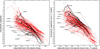 |
Fig. 1 GRB afterglow sample from 2008 to 2021. Left panel: the observer frame light curves. These have been corrected for Galactic foreground extinction as well as, where applicable, the host-galaxy contribution and the supernova contribution. Light-gray curves represent the pre-Swift and Swift era samples of K6, K10, K11 (Type II GRB afterglows only). Red curves represent new GRB afterglow light curves presented in this work. Thick black curves represent the ɀ ≳ 6 high-ɀ sample. These light curves have been constructed by using the intrinsic spectral slopes to extrapolate the magnitude from redder bands to the RC band, essentially assuming the Universe is completely transparent. For these, the GRBs are labeled. Right panel: GRB afterglow light curves when shifted to all originate from ɀ = 1. See text for more details. |
3.2 Extended early time sample
As we have shown that the luminosity of GRB afterglows at the targeted high redshifts are directly comparable to the lower-ɀ sample of K6, K10, K11, we can use those afterglows as proxies, shifting them to high-ɀ with our knowledge of the intrinsic spectral slope. We can then use them in lieu of actual high-ɀ GRB afterglows, assuming they are detected at an early enough time, hereby greatly increasing our sample. We not only shift them in terms of distance and time, but also shift them to NIR bands, which, at the target redshift, are not affected by Lyman damping. These are: J@z = 5, J@z = 6, H@z = 8, K@z = 10, and K@ɀ = 15. However, almost all pre-Swift afterglows are useless for this exercise as their initial detections are too late. Only GRB 990123 and its extremely early prompt flash (Akerlof et al. 1999) can be used directly, for GRBs 021004 and 021211, we are able to back extrapolate the data in a secure manner and add them to the sample as well. We note that such a back extrapolation may yield a result that is not only insecure by up to 0.5 mag, but may be even significantly incorrect, e.g., in the case where a well determined, smooth decay is back extrapolated, but in reality it experienced a steep rise and turnover shortly before the first actual detection. Of course, in such cases, there is no way to know this for a fact. Afterglows whose earliest behavior is a rise to peak are more secure, however, even in such cases, prompt emission linked variability may be superimposed, such as in the cases of GRBs 080603A (Guidorzi et al. 2011) and 161023A (de Ugarte Postigo et al. 2018b). However, we will come to see that most GRB afterglows are more luminous than the assumed detection threshold by margins so large that even a result dimmer by several magnitudes will not make a difference to the simple binary classification of “brighter than the threshold” or not.
The position of the injection frequency, the frequency at which the lowest energy electrons are radiating, could affect our analyses (Mangano et al. 2007). In general, even at relatively early times, the injection frequency is expected for typical afterglow parameters to be at lower frequencies than optical/NIR. However, in a few cases, afterglow spectra have been modeled including the crossing of the optical/NIR bands by the injection frequency. While a detailed modeling could be needed in those cases, we do not expect that our statistical conclusions could be affected by the injection frequency position in any relevant way.
The Type II GRB samples of K10, K11 extend to late 2009, however, many well-observed GRBs from 2008 and 2009 are missing as large swathes of their photometric data were still unpublished at the time. These samples yield a total of 31 GRB afterglows that can be used in our sample, but this is still a small number. We therefore undertook the task of mining the literature for events from the years 2008 to 2021 to add to this sample. These events need to fulfil the K6, K10, K11 criteria namely:
A well-measured redshift, to allow us to correctly model and subtract host-galaxy dust extinction, and determine the shift in magnitude dRc to ɀ = 1 (and the further magnitude shifts to the high-ɀ targets given above).
Multicolor detections to allow the creation of a usable SED for extinction determination (“Golden” or “Silver Sample” following K10).
A second set of criteria establishes this as the Early Light Curve Sample:
Detection of the afterglow at early times. This criterion was ad hoc, “by eye”, leading to some cases with a full analysis which, in the end, could not be included in the sample as the first detection was too late, and no secure back-extrapolation could be achieved. We still list the analyses of these afterglows in Appendix B.3 but point out they were not included in the rest of the study.
The existence of a publication in the literature featuring a well calibrated data set, and not just data from GCN Circulars5. The reason for this is twofold. For one, it has kept the literature mining within a reasonable scope, as such publications usually feature figures that allow a rapid evaluation of the quality of the light curve data, whereas GRBs with only GCN values only yield this information post facto, after collecting and plotting all available data. Secondly, such data from actual publications (usually from refereed journals, but some are from conference proceedings, which may not be refereed) generally yield a trustworthy “backbone”, which is often multicolor, against which other data can be compared. We make an exception for GRB 180720B, for which our team obtained well-calibrated multi-epoch, multicolor data, which we present here for the first time (see Sect. 3.3).
These selection criteria yield a total of 45 new afterglows in the sample, furthermore four GRB afterglows already published in K10/K11 were reanalyzed with additional data, and we add a further 14 GRB afterglows from a separate sample dealing with the SNe associated with GRBs (Kann et al. 2019a, 2024). These latter events are only studied in terms of their early afterglow luminosity here, we defer further analysis to a future publication.
The data are gathered, plotted, cleaned of outliers, and fit according to the methods detailed further above. Hereby, potential multicolor host galaxy and supernova data are taken into account, and the host galaxy and supernova contributions are then subtracted to yield pure afterglow light curves. These are then combined (individually for each GRB) into composite RC light curves using the derived normalization, fully analog to what has been described in K6, K10. These composite light curves are shown in red in Fig. 1 (left panel: observer frame and right panel: shifted to ɀ = 1). It can be seen that compared to the samples presented in K10, K11, several even less luminous GRB afterglows have been added, here we especially highlight GRB 120714B associated with SN 2012eb, which is, over a large time-span, the least luminous well-observed afterglow so far (Klose et al. 2019). Generally, however, the new sample is in excellent agreement with the distribution of the K6, K10, K11 samples, albeit with an increase in very early detections, which was the aim all along.
Any detailed discussion of salient light curve features is deferred to future publications. Here we concentrate on the early luminosity distribution. As it is expected that Gamow will typically be on target within 100 s and observe for 500 s, we derive the logarithmic meantime of 245 s post-trigger as the point in time where we derive the flux density. This is an observer-frame time point, and the higher the redshift of the GRB is, the earlier we are probing into the rest-frame evolution of the light curve, a circumstance which will make Gamow a powerful tool for probing the early relationship between prompt emission and rest-frame UV/optical emission. As most of our light curves exhibit regular evolution over this time span, deviations from this time point stemming from an asymmetric flux distribution over the exposure are expected to be low. Furthermore, this allows us to derive the flux density with a simple linear interpolation between the two measurements closest in time.
Finally, for the J@ɀ = 5, J@ɀ = 6, H@ɀ = 8, K@ɀ = 10, and K@ɀ = 15 light curve plots, we derive 116, 115, 95, 82, and 53 detections, respectively. We show one example in Fig. 2. We do not differentiate between the K6, K10, K11 samples and the new Early Light Curve sample anymore, but still highlight the high-ɀ GRB afterglows up to 2021. The red two-headed arrow represents the time span during which Gamow will take its initial finding chart, and it is placed at the expected 5σ detection limit of 15 µJy. It is clearly visible that almost all GRB afterglows which actually have follow-up at such early times are detectable by Gamow. Plots for the other filter-redshift combinations look very similar. As redshift increases, afterglows become fainter (distance increases) and stretch out (time dilation), but they also become more luminous as we move to redder filters. These effects cancel each other out for the most part, but the fainter/more stretched out effect dominates, implying it becomes harder and harder to detect enough afterglows. From a purely practical standpoint, the sample also decreases with higher red-shift as even very rapid observations now correspond to times which are after the 500 s initial finding chart. We also point out that a significant fraction of early afterglows show a rising behavior, implying they will be significantly fainter during the finding chart than purely by the effect of increasing distance. Therefore, it is an informed strategy for further follow-up with Gamow to obtain further and deeper finding charts, as the afterglow may not “pop up” until many hundred to perhaps several thousand seconds after the initial GRB, something that is discussed more in Sect. 6.2.
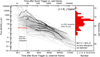 |
Fig. 2 Light curves of GRB afterglows and the sensitivity of the initial Gamow image. Afterglow light curves have been corrected for Galactic extinction, host extinction, and, where necessary, for the host-galaxy and supernova components. All afterglows are shifted to ɀ = 6 using knowledge of the intrinsic spectral slope, and flux densities have been converted to the J band. Thick black lines are the high-ɀ sample of GRB afterglows lying at ɀ ≳ 6. It can be seen that they agree with the distribution of afterglow luminosities at lower redshifts. The red horizontal bar with arrows represents the time span of the first image Gamow will take after slewing to a GRB position, a 500 s integration which we assume starts at 100 s after the trigger and reaches a limit of 15 µJy (21 mag in the AB system). The situation for the J band at ɀ = 5, the H band at ɀ = 8, and the K band at ɀ = 10, ɀ = 15 are similar, the time dilation and distance-induced luminosity decrease mostly cancel each other out for the higher redshifts. The distribution of afterglow brightness during the first 1000 s after the GRB trigger is shown in the histogram in the right panel. |
3.3 Additional data
To improve the results of our sample (e.g., additional filters), and especially to extend the number of early detections, here we analyze and present so-far unpublished data on a total of 40 GRBs.
Here, we highlight data sets for GRB 080413B (126 data points), GRB 080605 (104 data points), GRB 080721A (102 data points), GRB 081203A (144 data points), GRB 091018 (139 data points), GRB 091020 (111 data points), GRB 091208B (161 data points), GRB 100906A (230 data points), GRB 110213A (132 data points), GRB 131030A (261 data points), GRB 141221A (112 data points), GRB 150910A (109 data points), and GRB 180720B (132 data points), the last GRB not having a well-calibrated data set in the literature prior to this publication yet.
Observations have been obtained from these telescopes:
The Swift 30 cm modified Ritchey-Chretien UltraViolet/Optical Telescope UVOT (Roming et al. 2005), which yields data in three UV lenticular filters uυw2, uυm2, and uυw1, three optical filters u, b, and υ, and unfiltered (white). Early data are taken in “event mode” and can be split up into a finer time resolution.
The 0.6 m Rapid Eye Mount REM (Zerbi et al. 2001), equipped with the optical/NIR camera ROSS (Johnson-Cousins optical filters, 2MASS JHKS filters), and later the optical camera ROSS2 (SDSS filters) and the NIR camera REMIR (Z and 2MASS JHK filters), situated at ESO La Silla Observatory, Chile.
The 1.34 m lens/2 m mirror Tautenberg classical Schmidt telescope of the Thüringer Landessternwarte Tautenberg, Thuringia, Germany, equipped with a 2k × 2k CCD detector and Johnson-Cousins BVRCIC filters as well as a Z filter.
The 2.0 m Liverpool telescope (LT), equipped with RAT-Cam and SDSS filters, located at Observatorio Roque de los Muchachos (ORM), La Palma, Canary Islands, Spain (Steele et al. 2004), as well as its copies, the Faulkes Telescopes North (FTN) and South (FTS) located at Haleakalā Observatory, Maui, Hawaii, USA; and Siding Springs Observatory, New South Wales, Australia, respectively, as well as the 1.0 m telescope at McDonald Observatory, Texas, USA, which are now part of the Las Cumbrés Observatory Global Telescope (LCOGT) Network (Brown et al. 2013).
The 0.5 m D50, and the 0.25 m Burst Alert Robotic Telescope (BART, with Near-Field and Wide-Field detectors, NF, WF respectively; Jelínek et al. 2005) at the Astronomický ústav Akademie věd České republiky (AsÚ), Ondřejov, Czech Republic, yielding RC or unfiltered CR (calibrated to RC) observations.
The 0.4 m Watcher telescope, equipped with an RC filter or unfiltered, at Boyden observatory, near Bloemfontein, South Africa (Ferrero et al. 2010).
The 0.9 m T90 and 1.5 m T150 telescopes at the Obser-vatorio Sierra Nevada (OSN), Granada, Spain, equipped with Johnson-Cousins filters.
The 0.8 m Javalambre Auxiliary Survey Telescope JAST/T80, equipped with a 2 deg2 wide-field imager and SDSS filters (Cenarro et al. 2019).
Telescopes used by the team of the Seoul National University (SNU): the 1.0m LOAO telescope located at Mt. Lemmon Optical Astronomy Observatory, Tucson, Arizona, USA (Han et al. 2005; Lee et al. 2010). The 1.8 m Bohyunsan telescope at the Bohyunsan observatory, Korea, equipped with the Korea Astronomy and Space Science Institute Near-Infrared Camera System (Bohyunsan/KASINICS; Moon et al. 2008). The 2.1 m Otto Struve Telescope, located at McDonald Observa-tory,Texas, USA, equipped with the Camera for QUasars in EArly uNiverse (CQUEAN; Park et al. 2012). The 1.5 m AZT-22 telescope of Maidanak Observatory, Uzbekistan, equipped with the Seoul National University 4k× 4k Camera (SNUCAM; Im et al. 2010d). The UKIRT/WFCAM on Mauna Kea, Hawaii, USA (Casali et al. 2007).
A small number of data points have been acquired by the 8.2m Very Large Telescope equipped with the FOcal Reducer and low dispersion Spectrograph 2 (FORS2) and the X-shooter acquisition camera, Cerro Paranal, Chile, the F/Photometric Robotic Atmospheric Monitor (FRAM) at the Pierre Auger Observatory (PAO) in Malargue, Argentina, and the 1.0 m Anna L. Nickel telescope, Lick Observatory, California, USA. The 10.4 m Gran Telescopio Canarias (GTC) High PERformance CAMera (HiPERCAM) located at the Roque de los Muchachos Observatory on the island of La Palma, in the Canary Islands, Spain (Dhillon et al. 2021).
UVOT usually begins observing the fields of GRBs within the first minutes after the Swift/BAT trigger. Observations are typically taken in both event and image modes. In Table B.1, we only give data for certain filters for each GRB if there is at least one detection in that filter, in that case, all data, including upper limits, are presented. Before extracting count rates from the event lists, the astrometry was refined following the methodology of Oates et al. (2009). The source counts were extracted initially using a source region of 5″ radius. When the count rate dropped to below 0.5 counts s−1, we used a source region of 3″ radius. In order to be consistent with the UVOT calibration, these count rates were then corrected to 5″ using the curve of growth contained in the calibration files. Depending on the GRB, background counts were extracted using one or more circular regions located in source-free regions. The count rates were obtained from the event and image lists using the Swift tools uvotevtlc and uvotsource, respectively. They were converted to magnitudes using the UVOT photometric zero-points (Poole et al. 2008; Breeveld et al. 2011). To improve the S/N, the count rates in each filter were binned using ∆t/t = 0.1 or ∆t/t = 0.2, depending on circumstances, leading to longer but deeper exposures at later times. The early event-mode white and u finding charts were usually bright enough to be split into multiple exposures.
Ground-based photometry was generally analyzed using standard procedures: bias-subtraction, flat-fielding, and stacking, where necessary. Field calibration was obtained against on-chip comparison stars from the Sloan Digital Sky Survey (Alam et al. 2015) or the Pan-STARRS survey (Chambers et al. 2016). These values were either used directly for observations obtained in SDSS filters, or converted to Johnson-Cousins filters using the transformations of Lupton6. Zero point 1-sigma errors of the calibration are usually 0.02–0.07 mag, rarely higher. This systematic error is added in quadrature to the statistical measurement errors. NIR observations are calibrated against the 2 Micron All-Sky Survey 2MASS (Skrutskie et al. 2006).
The Tautenberg data of GRB 080605 had to be specially analyzed. This bright afterglow occurred in a crowded field, with a total of three stars nearby (Kann et al. 2008c). These stars were separated from the afterglow in VLT and LT/FTN images, but the large pixel scale of the Tautenberg camera  led to them being blended together. About 84 to 86 d after the GRB trigger, we revisited the field and acquired deep template imaging under good conditions in VRCIC. These template images were subtracted from fully reduced images containing the afterglow using the High Order Transform of PSF ANd Template Subtraction (HOTPANTS) software (Becker 2015). For S/N reasons, the three obtained V images as well as the four final IC images of the first epoch were stacked. All images in the second (RCIC) and third (IC only) epochs were stacked. The afterglow was not detected in the third epoch. In a few cases, the input images had a smaller PSF than the template images (in IC only). In these cases, as well as in the case of one further IC image where HOTPANTS did not converge, we modeled the PSF of stars in the image and used that model to subtract the two nearby bright stars. This leaves the afterglow as well as an even closer, faint star. We applied the PSF subtraction to the reference images, and determined the contribution of the faint third star, which was then subtracted in flux space. The derived Tautenberg magnitudes agree excellently with the contemporaneous LT measurements.
Reduction and analysis of data from the telescopes at AsÚ, namely the Ondřejov 0.5 m D50, the 0.25 m BART/NF (Nekola et al. 2010),WF, as well as the 0.3 m FRAM/PAO, are described in Jelínek et al. (2019), including the weighted image co-addition technique.
4 Theoretical approach via GRB simulations
The afterglow sample studied in this work is mostly composed of Swift/BAT bursts (with a few INTEGRAL GRBs, such as GRBs 161023A and 210312B, as this satellite also delivers positions with arcmin precision within seconds). Given its detection threshold, Swift/BAT introduces a redshift-dependent bias on the minimum luminosity of detectable GRBs. Any future mission design with improved sensitivity, like Gamow, will access less luminous GRBs than Swift/BAT. It is worth exploring how this systematic difference reflects on the afterglow luminosity in comparison to the current afterglow sample of GRBs detected by Swift/BAT.
The long GRB population is simulated following the prescription of Ghirlanda et al. (2015). We assume that the long GRB rate is ∝(1 + ɀ)δψ⋆(ɀ), where ψ⋆(ɀ) is the cosmic star formation rate (Li 2008) and δ = 1.7 (Salvaterra et al. 2012). GRBs are assigned a luminosity according to a broken power-law probability density function with low (high) end power-law slopes −1.3 (−2.5) and break L⋆= 1052 erg s−1. This function is defined within the limits [1046, 1056] erg s−1. In order to compute the flux of each simulated burst we assume a Band function (Band et al. 1993) for the prompt emission spectrum with low (high) energy spectral index assigned randomly from uniform distributions centered at −1 (−2.5) and standard deviation 0.1. We link the GRB luminosity to its rest frame peak energy via the Yonetoku correlation Log(Liso) = −27.02 + 0.57 Log(Epeak) (Yonetoku et al. 2004; Nava et al. 2012) where we account also for a 0.30 dex the scatter around this correlation. Similarly the isotropic equivalent energy is assigned following the Amati correlation (Amati et al. 2002; Nava et al. 2012) Log(Eiso) = −34.46 + 0.7 Log(Epeak) with a scatter 0.25 dex.
The afterglow emission is computed through the public code afterglowpy (Ryan et al. 2020) assuming distributions of the microphysical parameters as reported in Table 1 of Campana et al. (2022). By considering the Swift/BAT flux limit and Gamow LEXT instrumental design (Feldman et al. 2021), we compare in the right panel of Fig. 3 the distributions of the prompt-emission isotropic-equivalent energy Eiso of GRBs detectable by Swift/BAT (blue histogram) and LEXT (red histogram) at ɀ ~ 6. Owing to its softer energy range (0.3–5 keV) and better sensitivity, LEXT detects less energetic GRBs from all redshifts: there is a systematic difference of ~4 between the two distributions (the dashed blue line histogram shows the Swift distribution shifted by this factor).
Within the standard fireball model (e.g., Mészáros & Rees 1997), the afterglow luminosity depends on the outflow isotropic equivalent kinetic energy  which can be related to the prompt emission isotropic equivalent energy Eiso through the γ-ray emission efficiency parameter η. Moreover, afterglow emission depends on the external shock efficiency of accelerating relativistic particles and amplifying seed magnetic fields. Following the approach explained in Campana et al. 2022, we adopt the afterglow model of Ryan et al. (2020) to simulate afterglow emission produced in a constant density external medium7 by a uniform jet. The free model parameters regulating the shock micro-physics and the external medium density are calibrated by reproducing the afterglow flux density distributions of Swift GRBs in the X-rays (at 11 h) and optical (RC) bands at 600 s, 1, 11, 24 h of the BAT6 complete sample (D’Avanzo et al. 2014d; Melandri et al. 2014a).
The left panel of Fig. 3 compares the simulated afterglow flux density of GRBs at ɀ ~ 6 detectable by Swift (blue) and the observed sample of GRB afterglows collected in this work and redshifted to ɀ = 6 (solid filled gray histogram from Fig. 2). These two distributions have similar central values. The afterglow flux density distribution of GRBs detected by the Gamow at ɀ ~ 6 instead is on average dimmer by a factor ~6. This is mainly determined by the smaller kinetic energy (of which Eiso is a proxy) of bursts detected by LEXT. Indeed, by assuming a standard afterglow model, the flux in the optical-NIR band, sampling the frequency range between the maximum frequency and the cooling one (Starling et al. 2007; Greiner et al. 2003), should scale as  (Panaitescu & Kumar 2000) in the constant density external medium case, assuming all the other parameters are fixed. For a typical value of the shock-accelerated electron energy distribution p = 2.3 the difference between the Swift and Gamow isotropic energies (Fig. 3, right panel) accounts for the factor of 6 in the flux density distributions (Fig. 3, left panel). The corresponding rescaled flux density distribution is shown by the dashed blue histogram in the left panel of Fig. 3.
5 Results
5.1 The sensitivity of Gamow and the Early Light Curve sample
Using the results on the flux density at 245 s after trigger (observer-frame) that we derived for the Early Light Curve sample, we are now able to check how many early afterglows would be detected at at least 5σ significance by Gamow, depending on the band and the assumed redshift. Histograms for all five combinations studied here are shown in Fig. 4.
With the exception of the extreme case of K@z = 15 (so all the way up to K@ɀ = 10), we find that Gamow will recover 84%–86% of all early afterglows. We can also ask the inverse question: If we set the goal of 80% early afterglow recovery, what would the limiting flux densities PIRT needs to achieve? To do so, we simply check the flux densities of the GRB afterglow detections spanning the 80% demarcation, and do a linear interpolation. For example, for the J@z = 5 samples, we have 114 detections, so the brightest 91 detections contribute to the recovered sample, with the exact demarcation being 91.2. The 91st brightest afterglow is detected at 46.3 µJy, whereas the 92nd brightest is 39.4 µJy, a difference of 6.9 µJy, 20% of that is 1.4 µJy and thus the threshold is at 44.9 µJy. For the other filter-redshift combinations, we find 33.8 µJy, 35.2 µJy, and 30.3 µJy, respectively, and for K@ɀ = 15 we find 11.0 µJy, as for this sample PIRT with a sensitivity of 15 µJy is capable of recovering only 77% of all afterglows. In conclusion, overall, an 80% recovery rate with PIRT could be reached even if it is only half as sensitive, with a 5σ limit of 30 µJy in 500 s. However, as the true luminosity distribution of very high redshift GRB afterglows at early times is unknown (combined with the different sample in terms of prompt-emission properties LEXT will detect), and may indeed be fainter than our redshifted sample, as our simulations show, this should not be a place for cutting corners, and the 15 µJy limit provides a necessary safety margin.
The improved sensitivity and softer energy range extension of Gamow make it more efficient in detecting high redshift slightly fainter than Swift bursts. Based on the results shown in Fig.3, the theoretical approach leads to 70%–75% of recovery of all early afterglows by PIRT. However, this fraction may increase if there is a mild evolution of the characteristic luminosity of the GRB progenitors with redshift as recently found (Ghirlanda & Salvaterra 2022).
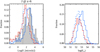 |
Fig. 3 Simulated GRB samples detectable by Swift and Gamow at z ~ 6. Right panel: distributions of the isotropic equivalent energy of simulated Swift (blue) and Gamow LEXT (red) GRBs. The dashed histograms in the right-hand panel corresponds to a rescaling of the Swift GRB distribution by a factor ~4 to reproduce the Gamow (red) distribution. Left panel: afterglow flux density distributions in the J band. This corresponds to the central frequency 1.84 × 10¹⁴ Hz of observed Swift GRBs (solid filled gray histogram from Fig. 2) compared with the distribution of J flux densities at 560 s (observer frame) of simulated Swift bursts (blue histogram) and simulated LEXT GRBs (red histogram). The dashed blue histogram shows the afterglow flux density rescaled by the energy factor ratio (see text). Dotted vertical line shows the flux density threshold of 15 µJy. |
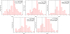 |
Fig. 4 Distribution of early GRB afterglow luminosities. These are measured at 245 s, the logarithmic center of an observation stretching from 100 s to 600 s after the trigger in the observer frame. The legends indicate to which redshiſt and which band the afterglows have been shifted, as well as the number of afterglows that are brighter than 15 µJy. The vertical dashed lines show the 15 µJy sensitivity requirement. The dotted vertical dashed line shows the flux threshold required to recover 80% of redshiſts, which exceeds the requirement for all but ɀ ≃ 15. |
6 Discussion
6.1 Meeting the Gamow requirements
Our results using past observations of GRB optical-NIR afterglows transformed to high redshift combined with the photo-ɀ simulations of Fausey et al. (2023) demonstrate that a space-based NIR multiband telescope with a sensitivity of 15 µJy in 500 s can provide photo-ɀ measurements with sufficient precision to determine whether or not a GRB is from high redshift ɀ > 5. This can be achieved with a modest 30 cm diameter telescope, cooled to below 210 K to eliminate its thermal radiation for sensitivity out to 2.4 microns (Seiffert et al. 2021).
This result is based on past observations, which will have selection biases. Gamow with a lower energy response for the LEXT compared to traditional GRB detectors will be sensitive to lower isotropic luminosity GRBs, especially at high redshift. K11 and K10 show that there is a mild correlation between prompt isotropic bolometric luminosity and the Rc band afterglow at 1 day, with an order of magnitude lower over three orders of magnitude of GRB luminosity. As noted by K11 there is almost a factor of 200 (over 5 mag) scatter in optical magnitude for a given GRB luminosity (see Fig. 13 in K11), most likely caused by differences in the jet viewing angle and circumstellar material. As a further validation our population modelling combined with a simple theoretical model for the jet interaction with a uniform circumstellar material shows that at most there is a overall factor of 4 lower average isotropic bolometric luminosity, and overall a factor of ~6 flux reduction, which is also consistent with the large scatter in the K11 Fig. 13. Even in this worst case scenario, the 15 µJy sensitivity threshold recovers ≈75% of the ɀ > 5 GRBs.
Another concern is that while the comparison sample is corrected for extinction, there maybe dust in the high redshift host galaxies which may impact the predictions. In the rest-frame (F)UV even small amounts of LOS extinction can have a large impact. Potentially GRB which would be only “somewhat extinguished” at low-ɀ become invisible at high-ɀ. This complete sample analysis suggest there cannot be a large number of dusty high-ɀ GRB host galaxies – which maybe consistent with the expectation of less dust at high redshift. JWST observations will likely provide more constraints on dust formation at high redshift.
6.2 Follow-up strategies with Big Glass and JWST
Figure 5 shows the distribution of flux-density at 4.7 h, 12 h and 3 days (observer-frame) after the GRB trigger of the ɀ = 8 H band sample. 4.7 h was used based on concept of operations simulations which show that this is the average time for one of the three major observatory sites to become available for Gamow detected GRBs. Also shown are approximate sensitivities with a 6m-10m NIR spectroscopy with ~2500 resolution and a S/N of ~20 per spectral resolution element in a few hours exposure. From this, it is clear that for the current largest telescopes it is essential to begin spectroscopy within a few hours. For the coming 25 m to 40 m telescopes this can be relaxed to ~12 h. Follow-up by JWST using a 3 days disruptive TOO is feasible for a large fraction of high-ɀ GRBs. A cascading strategy would be to first attempt spectroscopy from the ground, then trigger JWST if the former does not succeed because of weather, badly placed atmospheric telluric lines or being simply too high a redshift (where JWST excels).
It is important to note that cosmological dimming is offset almost completely by the time-stretching involved in increased redshift. As an example, we studied the luminosity sample for the “detected” sample at two days after redshift notification (2.011 d after trigger), and find for J@ɀ = 6 a mean and standard deviation:  mag. For H@ɀ = 8, it is:
  mag. And for K@ɀ = 10, it is:
  mag. We also derived mean magnitudes of the sample (in this case the representative H@ɀ = 8 “detect” sample) for even later times to check the feasibility of JWST follow-up at 5, 10, and 14 d, the latter case representing the time delay when a ToO request to JWST does not fall into the disruptive ToO category (which are limited in number). We find
  , respectively. Using again H < 24 mag as a threshold for useful spectroscopy from JWST, we find that 69% (50/72), 41% (24/59), and 32% (16/50) are still bright enough, respectively. Hence, while a not insignificant portion of GRB afterglows remain viable spectroscopic targets for JWST even two weeks after the GRB, the sample becomes increasingly biased toward the brightest afterglows. Additionally, as the afterglow evolution cannot be predicted, even initially bright afterglows should, for best results, be observed within the first week after the GRB.
7 Summary and conclusions
We took a large sample of GRB optical and NIR afterglows from 2008 to 2021 and used them to predict the expected afterglow brightness verses time for GRBs from high-ɀ (ɀ > 5). This sample is used to set the requirements for future GRB missions optimized to find high-ɀ GRBs and use them for cosmological studies of early star formation, galaxy evolution, metal enrichment, and reionization. We compared our findings to predictions from population studies combined with theoretical predictions and find good agreement. Our conclusion is that for future missions designed to survey and then use high-ɀ GRBs for cosmology, an onboard NIR telescope with multiband filters such as PIRT is essential in order to carry out the following functions:
- 1.
Determine for every GRB whether there is a sufficiently bright IR afterglow that can be spectroscopically followed up with large-telescope (>6 m) observatories.
- 2.
Determine the redshift of the IR afterglow to flag which of many hundreds of GRBs are from high redshift in order to identify the few high-ɀ objects worthy of follow-up observation.
- 3.
Determine the position of the IR transient with sufficient accuracy that a large ground-based telescope can directly follow up and place the afterglow in the spectrometer slit.
- 4.
Do all of this within 1000 s, so that spectroscopy of the afterglow can start when the afterglow is bright; and if possible within 1 h.
We conclude by noting that these capabilities will continue the legacy of Swift (Gehrels & Cannizzo 2015) and will address many astrophysics questions in tandem with new ground-based facilities such as the Vera Rubin Observatory, and future gravitational wave observatories.
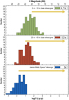 |
Fig. 5 Flux-density distributions at different observer-frame time points of the ɀ = 8 H band sample. These represent a 4.7 h ground-based reaction with current 6 m to 10 m class telescopes (top panel), a 12 h reaction with future 25 m to 40 m telescopes (middle panel), and a 3 days disruptive TOO reaction by JWST (bottom panel). With the arrows, we indicate the magnitude span over which each of the indicated telescope classes can acquire the required NIR spectrum (~ 2500 resolution) with a few hour integration time. |
Acknowledgements
Based in part on observations made at the Sierra Nevada Observatory, operated by the Instituto de Astrofísica de Andalucía (IAA-CSIC). D.A.K. acknowledges support from Spanish National Research Project RTI2018-098104-J-I00 (GRBPhot). D.A.K. is indebted to U. Laux, C. Högner, and F. Ludwig for long years of observational support at the Thüringer Landessternwarte Tautenburg, and S. Ertel, M. Röder, H. Meusinger, as well as A. Nicuesa Guelbenzu for observation time and further support. A.d.U.P. and C.C.T. acknowledge support from Ramón y Cajal fellowships RyC-2012-09975 and RyC-2012-09984 and the Spanish Ministry of Economy and Competitiveness through projects AYA2014-58381-P and AYA2017-89384-P, A.d.U.P. furthermore from the BBVA foundation We thank T Sakamoto, M Jang, Y. Jeon, M. Karouzos, E. Kang, P. Choi, and S. Pak for either assisting us obtaining the UKIRT, LOAO, Maidanak, and McDonald data for their role in securing the observational resources. M.I. and G.S.H.P. acknowledge the support from the National Research Foundation (NRF) grant nos. 2020R1A2C3011091 and 2021M3F7A1084525, and the KASI R & D program (Program No. 2020-1-600-05) supervized by the Ministry of Science and ICT (MSIT) of Korea. H.D.J. was supported by the NRF grant nos. 2022R1C1C2013543 and 2021M3F7AA1084525, and Y.K. was supported by the NRF grant no. 2021R1C1C2091550, both funded by MSIT. Y.K. was supported by the National Research Foundation of Korea (NRF) grant funded by the Korean Government (MSIT) (nos. 2021R1C1C2091550 and 2022 R1A4A3031306). M.M. acknowledges financial support from the Italian Ministry of University and Research -Project Proposal CIR01_00010. This research was funded in part by the National Science Center (NCN), Poland under grant number OPUS 2021/41/B/ST9/00757. This work made use of data supplied by the UK Swift Science Data Centre at the University of Leicester. The Pan-STARRS1 Surveys (PS1) and the PS1 public science archive have been made possible through contributions by the Institute for Astronomy, the University of Hawaii, the Pan-STARRS Project Office, the Max-Planck Society and its participating institutes, the Max Planck Institute for Astronomy, Heidelberg and the Max Planck Institute for Extraterrestrial Physics, Garching, The Johns Hopkins University, Durham University, the University of Edinburgh, the Queen’s University Belfast, the Harvard-Smithsonian Center for Astrophysics, the Las Cumbres Observatory Global Telescope Network Incorporated, the National Central University of Taiwan, the Space Telescope Science Institute, the National Aeronautics and Space Administration under Grant No. NNX08AR22G issued through the Planetary Science Division of the NASA Science Mission Directorate, the National Science Foundation Grant No. AST-1238877, the University of Maryland, Eotvos Lorand University (ELTE), the Los Alamos National Laboratory, and the Gordon and Betty Moore Foundation. Funding for SDSS-III has been provided by the Alfred P. Sloan Foundation, the Participating Institutions, the National Science Foundation, and the U.S. Department of Energy Office of Science. The SDSS-III web site is http://www.sdss3.org/. SDSS-III is managed by the Astrophysical Research Consortium for the Participating Institutions of the SDSS-III Collaboration including the University of Arizona, the Brazilian Participation Group, Brookhaven National Laboratory, Carnegie Mellon University, University of Florida, the French Participation Group, the German Participation Group, Harvard University, the Instituto de Astrofísica de Canarias, the Michigan State/Notre Dame/JINA Participation Group, Johns Hopkins University, Lawrence Berkeley National Laboratory, Max Planck Institute for Astrophysics, Max Planck Institute for Extraterrestrial Physics, New Mexico State University, New York University, Ohio State University, Pennsylvania State University, University of Portsmouth, Princeton University, the Spanish Participation Group, University of Tokyo, University of Utah, Vanderbilt University, University of Virginia, University of Washington, and Yale University. This work includes the data taken by the Mt. Lemmon Astronomy Observatory 1.0 m and the Bohyunsan Optical Astronomy Observatory 1.8 m telescope of the Korea Astronomy & Space Science Institute (KASI), the 2.1 m Otto-Struve telescope of the McDonald Observatory of The University of Texas at Austin, and UKIRT which was supported by NASA and operated under an agreement between the University of Hawaii, the University of Arizona, and Lockheed Martin Advanced Technology Center; UKIRT operations were enabled through the cooperation of the Joint Astronomy Centre of the Science and Technology
Appendix A Redshift Measurement Delays
The question might be asked Why not do this from the ground using e.g., the existing assets utilized in this work? The answer to this can be found by analysing the Swift percentage of redshifts recovered and the delay time to broadcast them for follow-up spectroscopy by large telescopes.
While Swift has proved exceptionally efficient at providing prompt gamma-ray (~ 2′ – 3′), X-ray (~ 2″ – 3″) and often UV/optical  localization of GRBs, it has in the vast majority of cases been reliant on ground-based follow-up to determine the GRB redshift with only ~ 30% recovered (Perley et al. 2016b).
In some cases a detection by Swift UVOT does provide rapid limits on the redshift. The white light filter typically used for finding charts is most sensitive in the UV, and cuts out at around 7000 Å. Hence, a UVOT detection is immediately indicative of ɀ < 5, with the most distant GRB detected by UVOT being GRB 060522 (Fox et al. 2006; Holland 2006) at redshift ɀ = 5. 11 (Cenko et al. 2006). However, the converse is not true. While > 50% of Swift detected GRBs are undetected by the UVOT, only a small fraction of these lie at ɀ > 5. The majority of non-detections are the result of either observations of insufficient depth, where the extrapolation of the X-ray flux to the optical lies below the available upper limits, where appropriate ground-based telescopes were unavailable because of weather, downtime, sky location or lack of time allocation to GRB science, or where intrinsic extinction renders the optical afterglow too faint, so called dark GRBs (Jakobsson et al. 2004; Rol et al. 2005; Greiner et al. 2011; Melandri et al. 2012).
A consequence of this is that any robust redshift measurements are substantially delayed from the time of the burst trigger. Such delays have significant implications for the ability to plan follow-up. It is much more straightforward to recover the GRB redshift with earlier data when the afterglow is brighter. The situation for high-ɀ bursts is even more acute, since NIR spec-troscopy is not routinely attempted. Hence, the afterglow must first be identified as a high-ɀ candidate via imaging observations and then targeted for NIR spectroscopy.
To quantify this effect we retrieved relevant times via a search of the GCN archives for all Swift bursts. Fig. A.1 gives an overview of the number of redshifts determined each year since the launch of Swift and the telescopes used to obtain them. The number of redshifts retrieved has clearly decreased as the mission has continued, while the GRB detection rate has maintained a comparable rate of between ~ 80 and 100 GRBs yr−1.
Where possible we record both the time of observation either from the GCN or available archives, and the time of dissemination to the community. Where recovery of the observation time is not possible we set it equal to the report time. We did not include observations obtained within the first days but only reported via papers that appear much later (months to years after the GRB) because they were not, for whatever reason, promptly reported to the community.
Fig. A.2 and Fig. A.3 show the delay times for all Swift bursts, both in terms of the time to observation, and of reporting to the community. The mean and median delays to observations are 29 and 5.5 hours (with the mean significantly skewed by a handful of very long delay times), and the 90% range 0.3 – 200 hours. For reports to the community the corresponding mean and median times are 45 and 11.8 hours with 90% of the reports coming within 2 –200 hours. It is important to note that the earliest robust indications of a redshift (photometric or spectro-scopic) are not reported to the community for > 1 hour after the burst. For the high redshift bursts, the situation is further complicated by the requirement to first identify IR counterparts before acquiring spectroscopy.
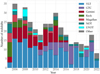 |
Fig. A.1 ber of redshifts obtained each year since the launch of Swift. The histograms are color-coded by the telescope that obtained the redshift measurement. |
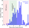 |
Fig. A.2 Delays in obtaining redshifts for GRBs in the Swift era. Highlighted are the time spans during which PIRT is expected to measure photo-ɀs on-board and transmit them to the ground, as well as our planned rapid follow-up observations. |
In Fig. A.4 we show timelines for all bursts in our high-ɀ sample with spectroscopic or photometric redshifts of ɀ ≳ 6. The mean and median delays here are not substantially different to those for the population of bursts as a whole. However, this is skewed low because for bursts at ɀ ~ 6 ɀ′-band detections are still possible, enabling direct spectroscopy, in some cases with optical spectrographs (e.g., Kawai et al. 2006). For example, the X-shooter instrument has provided more GRB red-shifts than any other, but acquires with an optical camera. In the case of ɀ ~ 6 bursts it can therefore, on occasion, obtain rapid spectroscopy, as was the case for GRB 210905A (Rossi et al. 2022). For bursts which require IR spectroscopy none was attempted at < 12 hours, and in each case, not at the same site as the initial photometric identification as a high–ɀ candidate.
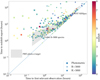 |
Fig. A.3 Delays between the time when a redshift was recorded vs. when the first relevant observation was obtained. We differentiate between redshifts that are only photometric, those that have been obtained by low-to-medium resolution spectrographs (resolution R< 3000) and those that have been obtained by medium-to-high resolution spectrographs (R> 3000). For each observation, the redshift itself is color-coded. Finally, with gray areas, we highlight the expected observation and report times for the initial PIRT observation, our planned follow-up with large ground-based facilities, and planned follow-up with JWST NIRSpec. |
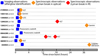 |
Fig. A.4 Timelines of the redshift determination for ten high-ɀ GRBs in the ɀ ≳ 6 sample. Two of these only have relatively insecure photometric redshifts. Three further ones were so distant that the Lyman-α line lies in the infrared and only low-S/N spectra allowing a redshift determination and little else could be obtained. In the other cases the Lyman-α line still lies in the optical regime and higher-quality spectra were usually obtained (especially for GRBs 130606A, 140515A, and 210905A). |
Having quantified the actual delays in obtaining observations, it is also relevant to consider their origin. The majority of the redshifts for GRBs reported in the literature arise from ground-based observations. Only in a handful of cases were there Swift UVOT grism observations (three events, Kuin et al. 2009; Kuin & Swift/UVOT Team 2019, 2021), or UVOT determined photometric redshifts (~ 15 events8). The delay to observations can therefore be decomposed into physical constraints and operational constraints. Once a burst is detected it takes some time before it becomes visible to a given observatory – such delays are unavoidable and can be many hours. The operational constraints then refer to the time to begin observations once the target is visible. A robust quantification of these issues is difficult because different telescopes have individual pointing constraints and the reasons for delays during visibility can also arise from varying sources (technical issues, weather, visiting astronomers, etc.).
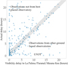 |
Fig. A.5 Actual delay time in obtaining redshift observations vs. the minimum possible delay. These are from the three premier observing sites La Palma, Chile, and Mauna Kea. GRBs apparently observed before the minimum possible delay (lower right) were observed by other observatories (e.g., in China or Russia) or by UVOT. Large delays despite being well-placed (top left) are usually down to weather or technical issues, instrumentation not being mounted or the lack of a redshift programme. |
To approximately understand the origin of the delays for Swift bursts we calculate the delay from the burst time until the source reaches 40 degrees of elevation with the Sun 18 degrees below the horizon at one of the following three: 1.) La Palma (Canary Islands, Spain), 2.) Chile (for which we adopt Cerro Paranal as a location) or 3.) Mauna Kea (Hawaii, USA), since these three sites are responsible for the vast majority of GRB redshift measurements. The resulting outcome is shown in Fig. A.5. A handful of bursts are apparently observed before the earliest possible observations. These cases are predominantly GRBs that had redshift measurements from other observatories including Swift UVOT. In some cases they are also cases where the burst was promptly visible at one of the three sites, but in twilight, or with an elevation < 40°. One feature that is clear from Fig. A.5 is that having redshifts and arc second positions determined onboard Swift by UVOT, reduces the delay time, so that when the afterglow does become visible to big glass these observatories can be ready to obtain the required spectra for high– ɀ GRBs, when the afterglow is still bright.
The China-France Space Variable Objects Monitor (SVOM) will launch in the near future and is predicted to detect ≈ 5 GRBs per year at ɀ > 5 by using a coded mask GRB detector in the X-ray band (Götz et al. 2009; Paul et al. 2011; Wei et al. 2016; Wang et al. 2020). SVOM carries an onboard Visible Telescope (VT) that is sensitive from 400-950 nm, considerably redder than the UV/Optical Telescope (VT) on Swift, which will provide rapid identification of optically dark afterglows. SVOM will rely on a network of ground-based telescopes to identify and obtain high resolution NIR spectra of the high redshift events. While the performance of this network is yet to be seen, it very likely will have the same challenges as Swift in obtaining rapid ground-based follow-up (telescope availability, weather, visibility, etc.) which means the rare high–ɀ events may be missed or observed too late to obtain high quality spectra.
Improvements in the speed of obtaining redshifts, and hence in redshift completion since bursts are brighter earlier, can therefore be obtained by three key improvements in the design of future programmes.
- 1.
GRB detectors should point at regions of sky that are promptly visible to large ground-based observatories. Although the duty cycle of large ground-based telescopes is not 100% there are relatively few gaps in the night time regions between the three major sites considered here. Therefore a pointing strategy which prioritises such visibility could potentially significantly improve delay times.
- 2.
Future GRB observatories should provide arc sec positions, accurate enough for direct spectroscopic measurements in the majority of cases.
- 3.
Since ground-based follow-up of premier facilities (e.g., ELTs) is very limited, missions should provide prompt and reliable indications of high redshift.
Gamow aims to maximize use of these strategies.
Appendix B Details on the new sample
Appendix B.1 Additional data added to the Swift-era sample
The following GRBs have data added that changes their light curves (usually at very early times) without changing the analyses presented in K10. For GRB 080319B, we added the high time resolution data of the prompt flare as measured by the TOR-TORA wide field camera presented by Beskin et al. (2010). We add V-band data presented by Brivio et al. (2022) to the light curve of GRB 080928. Page et al. (2019) present an analysis of Swift UVOT “settling images”, very earlytime υ-band detections. In the context of our sample, we add these data points to the light curves of GRBs 050922C, 060418, 060908, and 081008. Further GRBs are mentioned below in the context of our early-time sample.
Appendix B.2 The high–ɀ sample
Appendix B.2.1 GRB 050904, ɀ = 6.295 ± 0.002
Data are taken from Haislip et al. (2006); Tagliaferri et al. (2005); Kawai et al. (2006); Boër et al. (2006); Price et al. (2006); Berger et al. (2007); Gendre et al. (2007), and GCN Circulars (Perley et al. 2005). Deep host galaxy observations are presented in Berger et al. (2007); Tanvir et al. (2012a); Schulze et al. (2015); McGuire et al. (2016); Blanchard et al. (2016). The redshift is given by Kawai et al. (2006). The full analysis of this GRB afterglow has been done by Kann et al. (2007).
This GRB afterglow is characterized by a very early, extremely luminous (Kann et al. 2007) prompt flash and a reverse shock (Boër et al. 2006; Tagliaferri et al. 2005; Wei et al. 2006). The very luminous and extremely variable X-ray afterglow (Cusumano et al. 2006, 2007; Watson et al. 2006) has led to the interpretation that it belongs to the class of ultralong GRBs (Zou et al. 2006; Kann et al. 2018b). It was also highly luminous in the radio bands (Frail et al. 2006), and generally one of the most luminous GRBs observed to date (Sugita et al. 2009, K10). The presence or absence of dust along the line of sight to this GRB has been controversially discussed (Stratta et al. 2007, 2011; Zafar et al. 2010, 2011b; Liang & Li 2009), an interesting contrast to the very high column density in X-rays and evidence for dense surroundings (Campana et al. 2007; Gou et al. 2007).
Appendix B.2.2 GRB 080913, ɀ = 6.733
Data are taken from Greiner et al. (2009, see also Bolmer et al. 2018), Pérez-Ramírez et al. (2010). Deep host galaxy observations are presented in Tanvir et al. (2012a); Basa et al. (2012); Blanchard et al. (2016). The redshift is given by Patel et al. (2010). The full analysis of this GRB afterglow has been done by K10. The afterglow is relatively faint and shows a steady decay from early on (Greiner et al. 2009), which is followed by a very strong rebrightening (Greiner et al. 2009; Pérez-Ramírez et al. 2010). The GRB itself was quite short temporally, in contrast to the expected long lasting time dilated light curves such as in the case of GRB 050904. This led Zhang et al. (2009) to discuss the long/short nature of such GRBs.
Appendix B.2.3 GRB 090423, 
Data are taken from Tanvir et al. (2009, see also Bolmer et al. 2018), Yoshida et al. (2010b); Laskar et al. (2014). Deep host galaxy observations are presented in Tanvir et al. (2012a); Laskar et al. (2014); Blanchard et al. (2016). The redshift is given by Tanvir et al. (2009, see also Salvaterra et al. 2009). The full analysis of this GRB afterglow has been done by K10. The afterglow shows an extended early plateau phase (Tanvir et al. 2009; Yoshida et al. 2010b). Similar to GRB 080913, it was temporally short (Zhang et al. 2009).
Appendix B.2.4 090429B: 
Data are taken from Cucchiara et al. (2011c, see also Bolmer et al. 2018). Deep host-galaxy observations are presented in Cucchiara et al. (2011c); Tanvir et al. (2012a). The photometric redshift is given by Cucchiara et al. (2011c). This is the most distant GRB known to date. Data are very sparse. From the two K-band detections, we derive a decay slope α ≈ 0.6, in full agreement with Cucchiara et al. (2011c). The J band is strongly suppressed by Lyman damping, leaving only two filters to measure the SED. Without dust, we find β ≈ 1.14. While this value is not extraordinary, Cucchiara et al. (2011c) show via a joint NIR to X-ray fit that the cooling break must lie between the two spectral regimes, and that the intrinsic slope in the NIR range is β = 0.51 ± 0.17. Fixing this value, we derive AV = 0.23, 0.15, and 0.11 mag for MW, LMC, and SMC dust, respectively. Owing to the high-ɀ nature of the GRB, we prefer SMC dust, our value being in excellent agreement with the more detailed fitting procedure from Cucchiara et al. (2011c). We find the afterglow luminosity is very close to that of the GRB 090423 afterglow.
Appendix B.2.5 GRB 100905A, 
Data are taken from Bolmer et al. (2018), and GCN Circulars (Im et al. 2010a). Deep host-galaxy observations are presented in Bolmer et al. (2018). The (photometric) redshift is given by Bolmer et al. (2018). This GRB has very sparse data, with only two epochs of JHK detections. Bolmer et al. (2018) derive a photometric redshift from GROND data. We find the afterglow exhibits a shallow decay, α = 0.29 ± 0.09, which is shallower than that reported by Bolmer et al. (2018). It is indeed so shallow that the late upper limit on a host galaxy also implies that a light curve break must have occurred. Assuming a fixed break immediately after the GROND epoch at 0.658 d, we find α2 ≳ 0.88, which does not yield strong evidence that this break is a jet break. The large errors in the data lead to an insecure spectral slope, we find the JGHGKG SED can be fit by a simple power-law with no extinction and β = 0.48 ± 0.73, in excellent agreement with Bolmer et al. (2018).
Appendix B.2.6 GRB 120521C, ɀ = 6.15
Data are taken from Laskar et al. (2014), where we follow their correction of the ɀ′-band flux. We also present early RCICZ upper limits from observations with the Tautenberg Schmidt, first reported in Kann et al. (2012). The redshift is given by Laskar et al. (2014), based on a very low-S/N spectrum which shows a Lyman-α cutoff. The light curve shows a long rise and likely a smooth rollover to the decay. We fix n = 2 and find α1 = −0.84 ± 0.26, α2 = 0.96 ± 0.11, tb = 0.248 ± 0.049 d. We find a very similar α1 to Laskar et al. (2014), but a somewhat earlier break time, and shallower post-break decay slope α2, however, they still agree within errors. We follow the best-fit of Laskar et al. (2014) and fix β = 0.34, and derive a small amount of extinction, AV = 0.13 ± 0.03 mag from the ɀ′JHK SED, using SMC dust.
Appendix B.2.7 GRB 120923A, 
Data are taken from Tanvir et al. (2018). We also present upper limits from the 1.8m (Bohyunsan/KASINICS) in Korea, first reported in (Im et al. 2012). The redshift is given by Tanvir et al. (2018), based on a very low S/N spectrum which shows a Lyman-α cutoff. Deep host-galaxy observations are presented in Tanvir et al. (2018); Blanchard et al. (2016). We find that similar to several other high-ɀ GRB afterglows, that of GRB 120923A exhibits an early plateau phase. We find α1 = 0.06 ± 0.09, α2 = 1.96 ± 0.29, tb = 1.59 ± 0.33 d. This implies Δα = 1.89 ± 0.30, an unusually large value (Zeh et al. 2006). The JHK SED is modeled perfectly well by a simple power-law with no dust extinction and β = 0.54 ± 0.48.
B.2.8 Appendix GRB 130606A, ɀ = 5.91285 ± 0.00002
Data are taken from Castro-Tirado et al. (2013); Littlejohns et al. (2014, 2015); Hartoog et al. (2015); Bolmer et al. (2018), from GCN Circulars (Masi & Nocentini 2013; Nagayama 2013; Morgan 2013b; Perley & Cenko 2013a; Trotter et al. 2013a,b; Klotz et al. 2013), as well the 2.0 m LT/FTN (first reported in Virgili et al. 2013b,c) and 1.0m LOAO observations (first reported in Im et al. 2013). Deep host galaxy observations are presented in McGuire et al. (2016). The redshift is given by Hartoog et al. (2015, see also Chornock et al. 2013; Castro-Tirado et al. 2013; Totani et al. 2014, 2016). This GRB has the second most luminous afterglow among the high-z sample, and was studied in great detail spectroscopically (Chornock et al. 2013; Castro-Tirado et al. 2013; Hartoog et al. 2015; Totani et al. 2014, 2016). The optical/NIR light curve is also, by far, the richest of the high-ɀ GRBs, and, similar to GRB 050904 (Boër et al. 2006), it was detected at early times by small (aperture < 0.5 m) robotic telescopes.
We find that the afterglow initially features a rise to an early peak, and a rollover into a decay phase. It is αrise = 0.972 ± 0.088, α1 = 1.591 ± 0.097, tb = 0.0076 ± 0.0009 d (657 ± 79 s), with n = 1 fixed. This fit yields a r′RCi′ɀ′ JHKS SED. At t ≈ 0.039 d, the afterglow transitions into a shallow decay phase before breaking again into a “normal” decay. It is αplateau = 0.502 ± 0.29, α2 = 1.807 ± 0.017, tb,2 = 0.160 ± 0.008 d, and n = 2 was fixed (we found n = 2.08 ± 0.53 when leaving it free, however, this leads to very large errors in the normalizations, so we fixed n when deriving the SED). This decay is 2.2σ steeper than α1, however, it is still likely that the plateau represents an energy injection and the decay after the end of the injection continues as before. The final ɀ′ data point lies significantly above the extrapolation of the earlier decay slope, indicating another rebrightening has probably taken place.
The second fit yields a gGrGr′RCi′Zz′YJGJHGHKSKG SED (gG being an upper limit only). We fit both SEDs simultaneously, leaving the normalizations free for each SED but sharing the other parameters. We find no evidence for any color evolution between the two SEDs. A fit without extinction is perfectly acceptable, and we find β = 0.886 ± 0.092. Fits with extinction in all cases yield similar spectral slopes and AV = 0 mag within errors. This is in full agreement with “Solution 3” of Littlejohns et al. (2014) and in good agreement (1.4σ) with the X-ray-to-optical fit shown in Hartoog et al. (2015), who also set an upper limit on the extinction of AV ≲ 0.2 mag. At ≈ 0.05 d, this is among the most luminous GRB afterglows ever detected, comparable to the dusty moderately high-ɀ GRB afterglows of GRB 080607 and GRB 140311A, as well as the strong rebrightening of GRB 081029.
Appendix B.2.9 GRB 140515A, ɀ = 6.3298 ± 0.0004
Data are taken from Melandri et al. (2015); Bolmer et al. (2018), and GCN Circulars (Fong et al. 2014). Deep host galaxy observations are presented in McGuire et al. (2016). The redshift is given by Melandri et al. (2015, see also Chornock et al. 2014).
The available data are fit by a simple power-law decay, however, later upper limits indicate a light curve break must have occurred. Furthermore, the earliest detections (Fong et al. 2014) lie somewhat above the back extrapolation of the later decay and were not included in the fit. Fixing the break time to tb = 1 d, we find α1 = 0.48 ± 0.23, α2 ≳ 1.67. This is qualitatively in agreement with the X-ray results presented in Melandri et al. (2015), who find tb ≥ 105 s and a very steep decay α2 = 3.9 ± 0.6. The prebreak slope we find is shallower than that given by Melandri et al. (2015), as they include the early detection (Fong et al. 2014), and use only their data, while we perform a joint fit together with the GROND data (Bolmer et al. 2018). The iGɀGJGHGKG SED (iGɀG are clearly affected by Lyman damping and are not included) is fit perfectly well by a simple power-law with no dust extinction and β = 0.22 ± 0.35, a very shallow spectral slope. From an optical to X-ray fit using their X-shooter spectrum, Melandri et al. (2015) derive β = 0.33 ± 0.02 and AV = 0.11 ± 0.02 mag.
Appendix B.2.10 GRB 210905A, ɀ = 6.312
This was a very energetic and long high-ɀ event with many similarities to GRB 050904. All data, the redshift, and the full analysis are presented in Rossi et al. (2022); Saccardi et al. (2023). At late times, the afterglow is one of the most luminous ever detected (along with that of GRB 160625B Xu et al. (2016)).
Appendix B.2.11 Erratum on GNz-11 Flash
Jiang et al. (2021b) reported on a potential K-band flash detected in the spectral sequence of the lensed high-ɀ galaxy GN-z11, which they find to be at ɀ ≈ 11 (Jiang et al. 2021a). They interpreted this flash as associated with the prompt emission of a GRB. This led to intense discussion in the literature (Nir et al. 2021a,b; Padmanabhan & Loeb 2022; Steinhardt et al. 2021; Jiang et al. 2021c), before Michałowski et al. (2021) convincingly showed that it resulted from a satellite in Earth orbit crossing the spectrograph slit. In Kann et al. (2020), we showed that, assuming GN-z11 Flash is located at ɀ = 11, its brightness would be in agreement with the early UV/optical/NIR luminosity of transients associated with GRBs. While the association has been shown to very likely be incorrect, we here wish to point out one incorrect statement in that work. The first upper limit after the “flash” was also put into context, and it was stated the afterglow of this potential GRB had to be among the least luminous known so far. However, this continued to assume the spectral slope derived for the flash, which was extremely blue and not in agreement with usual GRB afterglow spectra. Applying a spectral slope in the typical range β ≈ 0.5 – 1.1, as expected for GRB afterglows, leads to a significantly larger dRc and therefore significantly shallower upper limits, e.g., for β = 0.6, it is dRc = −5.47 mag, whereas it is dRc = −1.98 mag for the spectral slope β = −1.2 which Jiang et al. (2021b) measure. Therefore, the upper limits do not impose a strong constraint on potential afterglow emission if it were to exist.
Appendix B.3 The early time afterglow sample
Appendix B.3.1 GRB 080413A, ɀ = 2.4330
Data are taken from Yuan et al. (2008), K10, from GCN Circulars (Klotz et al. 2008a; Fukui et al. 2008; Marshall et al. 2008), as well as our own Swift UVOT data (first reported in Oates & Marshall 2008), 0.6 m REM optical and NIR data (first reported in Antonelli et al. 2008), and 2.0 m LT and FTS data (first reported in Gomboc et al. 2008a), which are mostly upper limits with one unpublished low-significance detection. The redshift is given by Fynbo et al. (2009).
The analysis of this GRB afterglow was first presented in K10. Here, with expanded data from Swift UVOT, REM, and LT, we reanalyze the event. The early afterglow shows variability superposed on the general decay. Data beginning at 0.005 d can be fit well (χ2/d.o.f. = 1.29) with a smoothly broken power-law with α1 = 0.824 ± 0.038, α1 = 1.520 ± 0.030, tb = 0.015 ± 0.002 d, n = 10 fixed and no host galaxy contribution. The post break decay slope is in agreement with K10, whereas a different choice of starting time makes the prebreak slope different.
The SED (uBVRCICɀ′ JHK) is significantly broader than before, and now shows clear curvature. A fit without dust finds it to be moderately red, β = 1.17 ± 0.10 (χ2/d.o.f. = 1.58). A fit with MW dust shows that the 2175 Å is not detected, and therefore ruled out. LMC dust, with a smaller bump, is able to be accommodated, however, the fit yields high extinction and a strongly negative intrinsic spectral slope. K10 stated that SMC dust yielded the best result, which we confirm, however, a free fit yields an intrinsic spectral slope ≈ 0 (χ2/d.o.f. = 0.28). We fix the intrinsic spectral slope to a value derived from X-rays under the assumption νc lies between optical and X-rays, β = 0.55, and derive AV = 0.228 ± 0.037 mag (χ2/d.o.f. = 0.49). This value is larger than that derived for SMC dust in K10 (β = 0.52 ± 0.37, AV = 0.13 ± 0.17 mag), but consistent within errors. The somewhat larger value also leads to a larger correction, we find  . As already stated in K10, the early afterglow is one of the most luminous known, reaching nearly 9th magnitude in the ɀ = 1 system.
Appendix B.3.2 GRB 080413B, ɀ = 1.1014
Data are taken from Filgas et al. (2011b), from GCN Circulars (Brennan et al. 2008), as well as our own Swift UVOT data, first reported in Oates & Stamatikos (2008), and FTS data, first reported in Gomboc et al. (2008b). The data from Brennan et al. (2008) were made fainter by 0.7 mag to bring them into agreement with those of Filgas et al. (2011b). The redshift is given by Fynbo et al. (2009).
This burst was first analyzed in K11 with GCN and preliminary Swift UVOT data. It shows a decay turning into a long plateau phase, followed by a steep decay, and has been explained by a double-jet model (Filgas et al. 2011b). It also shows strong evidence for spectral evolution from a very flat to a “normal” spectral slope (Filgas et al. 2011b, K11).
With the full Swift UVOT data set, we confirm and expand these results, and fill the large data gap found in Filgas et al. (2011b). Our first fit covers data up to 0.1d. We find the early afterglow is best fit with a broken power-law decay, with a steep to shallow transition. It is α1 = 0.817 ± 0.022, α2 = 0.523 ± 0.011, tb = 0.0098 ± 0.0011 d (850.2 ± 96.8 s), n = −10 fixed and here we do not add a host contribution which is several magnitudes fainter. The fit is excellent, χ2/d.o.f. = 0.62. The second fit uses data beginning at 0.14 d (there is no data between 0.1 and 0.14 d) and we find: α3 = −0.009 ± 0.058, α2 = 2.39 ± 0.08, tb = 2.28 ± 0.14d, n = 1 fixed (a soft rollover), the host galaxy magnitudes for g′r′ were left free. Only these two bands show a transition into the host. Scatter in the data leads to a worse fit than the initial one (χ2/d.o.f. = 2.33). The first fit agrees very well with the result from K11, and the second fit yields the same α4 within errors, but the additional Swift UVOT data coverage shows a different behavior for the earlier part of this data set (a flat plateau instead of a decay similar to the earliest decay), and the break time is over a day earlier.
In both cases, the SED is very broad9, but the two show completely different behavior, as found before. The first SED shows some scatter, with especially b being too faint, the source of this offset is unclear as the second SED does not show this effect. The uvw2 uvm2 uvw1 bands are affected by Lyman dropout and are not included. We fit both SEDs simultaneously, fixing AV as a shared parameter, but not β. Without dust, we find β1 = 0.409 ± 0.047, β2 = 0.772 ± 0.046, with χ2/d.o.f. = 2.65. The result for the second SED is very similar to that found in K11, but the result for the early SED is steeper. This stems from the addition of the full UVOT u data set, which shows some curvature in the SEDs. For MW dust, we find slightly negative extinction (0 within errors). For LMC dust, the extinction is higher, but a 2175 Å bump is ruled out by the bright g′ band. The best fit is found for SMC dust, with β1 = 0.03 ± 0.14, β2 = 0.39 ± 0.14, AV = 0.23 ± 0.08 mag. The latter slope value agrees perfectly with the late-time XRT spectrum presented on the XRT repository if the cooling break lies between optical and X-rays. We find  , ≈ 0.44 mag brighter than the value found in K11.
Appendix B.3.3 GRB 080603B, ɀ = 2.6893
Data are taken from Jelínek et al. (2012), from GCN Circulars (Rujopakarn et al. 2008; Klotz et al. 2008c,b; Zhuchkov et al. 2008; Kuin & Mangano 2008; Xin et al. 2008; Miller et al. 2008; Klunko & Pozanenko 2008; Rumyantsev et al. 2008a; Ibrahimov et al. 2008), as well as our own observations from Swift UVOT (first reported in Kuin & Mangano 2008), from the Tautenberg (first reported in Kann et al. 2008a,b), and the LT (first reported in Melandri et al. 2008). The redshift is given by Fynbo et al. (2009).
This GRB afterglow features multiple phases and breaks in its light curve. The initial afterglow is reported to be “rapidly fading” (Rujopakarn et al. 2008) from an initial detection at mid-time 25.3 s. However, we find the afterglow to fade rapidly from the first detection of the white finding chart on, at 79 s, with a slope αsteep = 1.89 ± 0.10, a good indicator of reverse-shock flash behavior. During the first v observations, the afterglow transitions into a plateau phase, a behavior noted before (Klotz et al. 2008c,b). This is followed by dense multicolor coverage showing a further break, first reported by Zhuchkov et al. (2008) and confirmed by Jelínek et al. (2012). We find α1 = 0.436 ± 0.019, α1 = 1.147 ± 0.046, tb = 0.109 ± 0.006 d, n = 10 fixed and no host-galaxy contribution. Within errors, this is fully in agreement with Jelínek et al. (2012) and also similar to the results of Zhuchkov et al. (2008). The afterglow then breaks for a final time during a gap in data coverage, and later observations show it to decay steeply, with α3 = 2.35 ± 0.20, as first noted by Kann et al. (2008b). This latter break very likely represents a jet break. The earlier break may stem from the cessation of energy injection into the afterglow.
The SED is broad (uvw1 ubg′vr′RCi′JHKS) and straight. uvw1 ubg′ are affected by Lyman dropout and are not included. Fits with dust find very small values, all 0 within errors (negative for SMC dust). We prefer a fit without dust and a spectral slope β = 0.621 ± 0.068 (χ2/d.o.f. = 0.74). This agrees fully within errors with the value derived by Jelínek et al. (2012). For this fit, we find  .
.
Appendix B.3.4 GRB 080605, ɀ = 1.6403
Data are taken from Zafar et al. (2012); Jelínek et al. (2013), from GCN Circulars (Clemens et al. 2008; Rumyantsev & Poza-nenko 2008), as well as our own analysis of Swift UVOT data (first reported in Holland & Sbarufatti 2008; Kuin et al. 2008), Tautenburg observations (first reported in Kann et al. 2008e,d,c, see Sect. 3.2 for the special analysis done for this data), 2.0 m LT and 2.0 m FTN observations (first reported in Gomboc et al. 2008c), and 8.2m VLT/FORS2 spectroscopy acquisition images (first reported in Jakobsson et al. 2008). Host galaxy observations have been taken from Krühler et al. (2012); Blanchard et al. (2016); Lyman et al. (2017). The redshift is given by Fynbo et al. (2009).
This was a bright burst in a crowded field with high line-of-sight extinction and a clear 2175 Å bump in the spectrum (Zafar et al. 2012). The afterglow shows a steep-shallow-steep evolution. We find αsteep = 1.344 ± 0.017, α1 = 0.620 ± 0.005, tb = 0.00575 ± 0.00021 d (tb = 487 ± 18 s), n = −10 fixed (χ2/d.o.f. = 3.23 owing to some scatter). The early decay compares well with the result Jelínek et al. (2013) find, αsteep = 1 .27 ± 0.04, based on a smaller data set. Using data after 0.0076 d, we find α1 = 0.535 ± 0.015, α2 = 0.782 ± 0.022, tb = 0.069 ± 0.013 d (tb = 5981 ± 1137 s), n = 10 fixed (χ2/d.o.f. = 2.26). This break is clearly not a jet break. To our knowledge, it has not been reported in the literature yet.
The SED derived from the second fit is broad (bgGg′vrGr′RCiGi′ICɀG JHK) and clearly red but not strongly curved, without dust we find β = 1.482 ± 0.079 (χ2/d.o.f. = 1.41). A fit with MW dust finds very little extinction and an intrinsic spectral slope that is still too red: β = 1.37 ± 0.21, AV = 0.085 ± 0.146 mag (χ2/d.o.f. = 1.51). LMC dust leads to a significantly bluer intrinsic spectral slope and higher extinction: β = 0.31 ± 0.45, AV = 0.78 ± 0.29 mag (χ2/d.o.f. = 0.92). We point out that the v band lies in the 2175 Å but does not support its detection. It is clearly seen in the X-shooter spectrum shown by Zafar et al. (2012), but not very deep, and their photometry does not actually cover it. Therefore, it may come as no surprise that our SED is also well-fit by SMC dust: β = 0.57 ± 0.35, AV = 0.51 ± 0.19 mag (χ2/d.o.f. = 0.84). Zafar et al. (2011a) find a large extinction value  mag with a full Fitzpatrick-Massa parametrization. Later studies do not support this large extinction, Zafar et al. (2012) find β = 0.60 ± 0.03,
  mag, and β = 0.60 ± 0.02,
  , for two different SEDs at different times, with RV = 3.24 ± 1.05 and
  , respectively. Greiner et al. (2011) derive β = 0.67 ± 0.01, AV = 0.47 ± 0.03 mag. These results are in good agreement with our SMC dust result, which we will continue to use henceforth. For this result, we find dRc = −2.473 ± 0.489 mag. The early afterglow in the ɀ = 1 system is luminous, with RC ≈ 11 .9 mag.
Appendix B.3.5 GRB 080721, ɀ = 2.5914
Data are taken from Starling et al. (2009); Page et al. (2019), from GCN Circulars (Chen et al. 2008; Huang et al. 2008), as well as our own Swift UVOT analysis (first reported in Holland et al. 2008; Ward et al. 2008). The redshift is given by Fynbo et al. (2009).
The GRB was already presented in K10, however, we here add the large and complete UVOT data set. We reaffirm a fit with a broken power-law as presented in K10, we find α1 = 1.192 ± 0.009, α2 = 1.53 ± 0.09, tb = 2.08 ± 0.89 d, n = 10 fixed and no host-galaxy contribution. This implies Δα = 0.34 ± 0.09, in agreement with the result of K10 within errors and still conform with a cooling-break passage.
The SED (uvw1ubvRCIC) is significantly improved compared to the analysis of K10. It is clearly Lyman-damped in uvw1u, so these bands are not included. The slope without dust is still red (β = 1.48 ± 0.12, χ2/d.o.f. = 0.83), but less so than in K10 (β = 2.36 ± 0.30). MW dust is ruled out as there is no indication of a 2175 Å bump in the IC band. A fit with LMC dust yields a viable result but the intrinsic spectral slope is significantly steeper than the X-ray slope βX = 0.86 derived by Starling et al. (2009), so we prefer the fit with SMC dust, just as K10 did, finding β = 0.65 ± 0.79, AV = 0.18 ± 0.17 mag,χ2/d.o.f. = 0.50. As a direct comparison, a fit with β = 0.86 fixed yields AV = 0.137 ± 0.025 mag, significantly less than the result of K10, AV = 0.35 ± 0.07 mag.
Using our new SMC result, we derive  mag, less than the K10 value of dRc = −3.68 mag. The earlier detection from Page et al. (2019) leads to a similar early peak magnitude of RC ≈ 9.2 mag, however. Therefore, GRB 080721 still has one of the most luminous early afterglows discovered so far.
Appendix B.3.6 GRB 081007, ɀ = 0.5295 ± 0.0001
Data are taken from Jin et al. (2013), Olivares E. et al. (2015, including unpublished higher time-resolution early GROND observations). Host-galaxy observations are taken from Vergani et al. (2015); Blanchard et al. (2016); Lyman et al. (2017). The redshift is given by Berger et al. (2008).
This was a moderately low-redshift GRB with dense follow-up and an associated, spectroscopically confirmed SN. The SED shows a blue intrinsic spectrum and a quite large amount of SMC dust extinction, AV = 0.82 ± 0.09. For this fit, we derive dRc = 0.377 ± 0.128 mag, the early afterglow peaks at RC = 15.7 mag.
Appendix B.3.7 GRB 081029, ɀ = 3.8479 ± 0.0002
Data are taken from Nardini et al. (2011); Holland et al. (2012), and from a GCN circular (West et al. 2008a). The redshift is given by Holland et al. (2012).
This GRB afterglow shows a very complex evolution which was followed up in detail by GROND (Nardini et al. 2011). The initial afterglow shows a shallow decay with a break to a more regular value, we find: αshallow = 0.420 ± 0.027, α1,a = 0.789 ± 0.017, tb = 0.01118 ± 0.00097 d(tb = 966 ± 84 s), n = 10 fixed (χ2/d.o.ƒ. = 0.85). This is followed by a very strong, fast rebrightening which turns over into a decay phase with superposed small-scale substructure. For this phase, we measure: αrise = −4.19 ± 0.18, α1,b = 0.707 ± 0.0069, tb = 0.05442 ± 0.00063 d, n = 1.68 ± 0.13 (χ2/d.o. ƒ. = 5.32 resulting from the above-mentioned deviations). The decay after the rise is similar to the decay preceding it. After a sharp break at 0.195 d, the afterglow decays steeply before turning more shallow again -this slope decrease would indicate a transition to the host galaxy, however, deep late-time observations (Nardini et al. 2011) do not reveal any host at the GRB position. We find: α2 = 2.019 ± 0.011, α3 = 0.97 ± 0.16, tb = 1.90 ± 0.25 d, n = −5 fixed (χ2/d.o.ƒ. = 2.61). As the afterglow is dominated by GROND data, Nardini et al. (2011) find values mostly in agreement with ours. For the early phase, they find αshallow = 0.38 ± 0.05, α1,a = 1.12 ± 0.06, the latter value being significantly steeper than our result. For the rise, they determine αrise ≈ −4.7, in general agreement with our value. They exclude flaring activity from the following decay and derive an underlying α1,b ≈ 0.47, shallower than our result. For the steep decay, they find α3 = 2.3 ± 0.2. When fitting the entirety of the light curve with a sum of broken power-law models, they find similar values except for the rise, which becomes much steeper, αrise = −8.2 ± 0.4. They explain the final flattening with the renewed detection of the early component α1,a. Together with color evolution, Nardini et al. (2011) interpret the light curve as the superposition of two separated and spectrally different components, with the first one becoming dominant again at late times as the second decays more rapidly.
As Nardini et al. (2011) detect a color change in the SED between the first and second component, we derive two SEDs and fit them separately. The first (gGrGRCi′GɀGJJGHGHKG) is determined from the first fit derived above, whereas the second (uvw2uvm2uvw1ubgGvrGRCi′GƒCɀGJJGHGHKGK are upper limits only) is derived from the fit the strong rise and following decay. Data blueward of the R bands is affected by Lyman-damping and is excluded. The SEDs show some scatter and clear curvature. Without dust, we find β = 0.869 ± 0.044 (χ2/d.o. ƒ. = 3.76) and β = 1.062 ± 0.011 (χ2/d.o.ƒ. = 30.54). The latter value is in perfect agreement with that of Nardini et al. (2011). The two SEDs are markedly different by 4.2σ, confirming the result of Nardini et al. (2011). A fit with MW dust finds negative extinction, whereas fits with LMC dust are generally viable, but find extremely blue (partially negative) intrinsic spectral slopes. Fits with SMC dust yield the best result, with β1 = 0.11 ± 0.20, AV,1 = 0.25 ± 0.06 mag (χ2/d.o.ƒ. = 1.89), β = 0.33 ± 0.05, AV,2 = 0.240 ± 0.016 mag (χ2/d.o.ƒ. = 5.00), respectively. The intrinsic spectral slopes agree within the large errors, however, Δβ is identical to the ft without dust. The derived AV for the two fits is in excellent agreement with each other, remaining constant as expected whereas the underlying slope changes. Nardini et al. (2011), using an X-ray-to-optical analysis, find a less-curved SED and therefore a redder intrinsic result and less extinction: β = 1.00 ± 0.01,  for SMC dust.
For the second, more precise SMC fit, we derive a large  . At ɀ = 1, the early afterglow is luminous (RC = 11 .6 mag). The strong rebrightening makes this one of the most luminous afterglows known at later times.
Appendix B.3.8 GRB 081203A, ɀ = 2.05 ± 0.01
Data are taken from Page et al. (2019), from GCN circulars (Andreev et al. 2008a,b; Volkov 2008; West et al. 2008b; Liu et al. 2008; Mori et al. 2008; Isogai & Kawai 2008; Rumyantsev et al. 2008b; Fatkhullin et al. 2008) as well as our own Swift UVOT analysis (first reported in De Pasquale & Parsons 2008). The redshift is given by Kuin et al. (2009).
This was a very bright GRB afterglow which yielded the first Swift UVOT grism spectrum which allowed the measurement of the redshift. It was already presented in K10 but here we add the full UVOT data set which improves especially the characterization of the early afterglow. It shows a well-detailed rise to a rollover peak followed by a simple power-law decay, we find: αrise = −3.13 ± 0.08, α1 = 1.549 ± 0.009, tb = 0.00434 ± 0.00006 d (tb = 375.0 ± 5.2 s), n = 1 fixed, and no host-galaxy contribution (χ2/d.o.ƒ. = 4.56 resulting from scatter and small error bars).
The SED (uvw2uvm2uvw1ubg′vRCIC) is significantly improved compared to the one used in K10. The UV filters and u are Lyman-damped and excluded. Also, g′ is anomalously low and not included. The goodness of the afterglow fit leads to small errors in the SED and increased χ2 values. For no extinction, we find β = 0.92 ± 0.05 (χ2/d.o. ƒ. = 5.17.) MW dust leads to negative extinction, and SMC dust yields an excellent fit but with a negative intrinsic spectral slope. LMC dust yields a viable result, β = 0.72 ± 0.17, AV = 0.10 ± 0.08 mag, but with a worse fit than without dust (χ2/d.o.ƒ. = .95). We follow K10 and use SMC dust, fixing the spectral slope to β0 = ΓX − 1 − 0.5 = 0.45, for this value we find AV = 0.127 ± 0.017 mag, fully in agreement with K10. For this fit, we derive  . The early peak rises to RC = 10.4 mag in the ɀ = 1 system.
Appendix B.3.9 GRB 090426, ɀ = 2.609
Data are taken from Antonelli et al. (2009); Xin et al. (2011); Thöne et al. (2011); Nicuesa Guelbenzu et al. (2011), from GCN circulars (Yoshida et al. 2009b,a; Mao et al. 2009a; Kinugasa et al. 2009a), and from our own Swift UVOT analysis (first reported in Oates & Cummings 2009). The redshift is given by Levesque et al. (2010).
This GRB was discussed widely in the literature as it has a very short duration, especially in the rest-frame, but is likely to be a Type II GRB (Antonelli et al. 2009; Zhang et al. 2009; Levesque et al. 2010; Xin et al. 2011; Thöne et al. 2011; Nicuesa Guelbenzu et al. 2011, K11). Nicuesa Guelbenzu et al. (2011) already showed the optical luminosity of the afterglow is compatible with a Type II origin. We therefore include this GRB in our sample.
The afterglow shows a complex evolution. After a potential initial sharp rise, the afterglow decays at a shallow rate before smoothly turning over into a steeper day (Xin et al. 2011). We find: αshallow = 0.20 ± 0.07, α1 = 1.177 ± 0.038, tb = 0.00236 ± 0.00026 d (tb = 203.9 ± 22.5 s), n = 3 fixed (χ2/d.o.ƒ. = 1.07). These values are fully in agreement with those of Xin et al. (2011), who find αshallow , = 0.26 ± 0.07, α1 = 1.22 ± 0.04, tb = 227 ± 27 s. Nicuesa Guelbenzu et al. (2011) also find values that agree well, except for a steeper initial decay: αshallow = 0.48 ± 0.04, α1 = 1.22 ± 0.05, tb = 290 ± 20 s (with n = 3 fixed). After a short plateau phase, at ≈ 0.06 d (Xin et al. 2011 find tb = 0.082 ± 0.042 d), the decay steepens again. The afterglow, following a data gap, shows complex behavior, which is likely comprise of a short, steep decay, another sharp rise, and then a clear steep decay that is likely post-jet-break (Nicuesa Guelbenzu et al. 2011). This variability, however, is not well-defined. Fitting data from 0.06 d onward, including the multicolor host-galaxy detections, we find α2 = 0.664 ± 0.020, α3 = 2.64 ± 0.11, tb = 0.497 ± 0.009 d, n = 10 fixed (χ2/d.o.ƒ. = 1.67). Our results also generally agree with those of Nicuesa Guelbenzu et al. (2011), who found: α2 = 0.46 ± 0.15, α3 = 2.43 ± 0.19, tb = 0.39 ± 0.02 d.
The SED is very broad (uvw2uvw1ubgGg′VrGRCiGICɀG JGHGKS), is straight and shows some scatter. Without dust, we find β = 0.850 ± 0.046. Fits with dust models yield negative extinction (SMC) or only small amounts of extinction compatible with 0 (LMC, MW). We therefore use the fit without extinction, This is fully compatible with Nicuesa Guelbenzu et al. (2011), who find β = 0.76 ± 0.14 and no evidence for extinction either.
Using the dustless fit, we find dRc = −2.488 ± 0.030 mag. The early peaks at RC = 13.8 mag.
Appendix B.3.10 GRB 090516, ɀ = 4.111 ± 0.006
Data are taken from Bolmer et al. (2018), GCN Circulars (Gorosabel et al. 2009; Christie et al. 2009), the automatic Swift UVOT analysis page (offline at time of writing, see Siegel & Rowlin-son 2009 for a preliminary report), and our own FTS data (first reported in Guidorzi et al. 2009), as well as VLT/FORS2 data (first reported in de Ugarte Postigo et al. 2009b). A late-time host galaxy observation has been taken from Greiner et al. (2015a). The redshift is given by de Ugarte Postigo et al. (2012).
This light curve has only been studied at late times so far. At early times, there is likely a rise following the first, faint white detection. Our afterglow discovery data from FTN shows the afterglow to be achromatically decaying with α1 = 1 .03 ± 0.06. This is followed by a large data gap, during which few observations were taken, however, the behavior reported by Coward et al. (2010) is contrary to known afterglow behavior (it would be an extreme flare with a very steep decay), so we do not implement this data. The afterglow is significantly recovered by the Liverpool Telescope and NOT (Gorosabel et al. 2009), and then GROND and VLT, at a magnitude only 0.5 mag fainter than the end of FTS observations and those of Stardome (Christie et al. 2009). It actually rebrightens a bit before going over into a steady decay with α2 = 1.551 ± 0.024. The final GROND data show it potentially flattening off to a host (Bolmer et al. 2018), which, however, would be exceedingly luminous at this high redshift. Bolmer et al. (2018) add this host component to their fit and therefore find a somewhat steeper decay than we do α2 ≈ 1.7.
The SED (gGrGRCiGi′ɀGJGHGKG) shows clear signs of a Lyman dropout affecting the bands blueward of iG. It furthermore shows curvature, and a red spectral slope without dust, β = 1.253 ± 0.034, χ2/d.o. ƒ. = 22.1. A fit with MW dust yields negative extinction, whereas free fits with LMC and SMC dust find negative spectral slopes and large extinction. Fixing the intrinsic spectral slope to a value derived from the XRT spectrum (β = 0.52), we find an improved but still formally unacceptable (χ2/d.o.ƒ. = 6.87) fit with SMC dust and AV = 0.250 ± 0.011 mag. The bad χ2 is a result of small errors, the fit looks satisfactory visually. Bolmer et al. (2018) find an intrinsically steeper slope (β = 0.97) but similar extinction (AV = 0.19 ± 0.03 mag). The moderately large redshift combined with the extinction leads to a large  . This large correction combined with the long plateau phase leads the afterglow of GRB 090516 to be one of the most intrinsically luminous at the late peak time of 0.124 d in the rest-frame.
Appendix B.3.11 GRB 090618, ɀ = 0.54
Data are taken from Cano et al. (2011); Page et al. (2011), and from GCN circulars (Updike et al. 2009a,b; Galeev et al. 2009). The redshift is given by Cenko et al. (2009). This was a very bright GRB at moderate redshift with a well observed, bright afterglow, also extensively studied in X-rays (Page et al. 2011; Campana et al. 2011). It has a prominent SN bump, but without spectroscopic confirmation (Cano et al. 2011). Using a fit with no dust extinction, we find dRc = +1.571 ± 0.006 mag, with a moderately luminous afterglow peak of RC ≈ 15.1 mag.
Appendix B.3.12 GRB 090726, ɀ = 2.713
Data were taken from Šimon et al. (2010), from GCN circulars (Moskvitin et al. 2009; Maticic & Skvarc 2009; Volnova et al. 2009; Kelemen 2009), and from our own Swift UVOT analysis (first reported in Landsman & Page 2009), as well as our own rereduction of the Ondrejov D50 data from Šimon et al. (2010) at a higher time resolution. This reanalysis does not recover the short flare Šimon et al. (2010) report. The redshift is given by Tanvir et al. (2019).
The afterglow is densely observed at early times but there is almost no data after 0.1 d. The early afterglow shows a rise and a long rollover to a relatively shallow decay before breaking to a steeper decay. We find αrise = −1.60 ± 0.12, α1 = 0.61 ± 0.03, tb = 0.00381 ± 0.00022 d (tb = 329 ± 19 s), n = 1 fixed (χ2/d.o. ƒ. = 2.21) for the early afterglow, and α1 = 0.55 ± 0.02, α2 = 1.49 ± 0.08, tb = 0.047 ± 0.0026 d, and n = 10 fixed, for the later afterglow. Šimon et al. (2010) undertake a different fit to their data but qualitatively find the same behavior.
The SED (ubvRC) is very red, and also u is affected by Lyman-damping, and we find β = 3.41 ± 0.60. Šimon et al. (2010) already pointed out that the RC band lies significantly under an extrapolation of the X-ray slope. The Swift XRT repository gives an X-ray slope of Γ − 1 = 1.30, which we adopt. The short baseline does not allow us to distinguish between dust models (the 2175 Å bump is insufficiently covered), and we conservatively use the SMC dust solution which has the lowest extinction, AV = 0.39 ± 0.11 mag (χ2/d.o.f. = 0.00006). For this fit, we find a large  . The corrected afterglow is luminous and peaks at Rc = 13.1 mag.
Appendix B.3.13 GRB 091018, ɀ = 0.9710 ± 0.0003
Data are taken from Wiersema et al. (2012); Page et al. (2019), from GCN circulars (Schaefer & Pandey 2009; de Ugarte Postigo et al. 2009c; LaCluyze et al. 2009a; Motohara et al. 2009; Cobb 2009a), and from our own Swift UVOT analysis (first reported in Landsman & Stamatikos 2009, our analysis includes early time-reseolved event mode data which was not given in Wiersema et al. 2012), as well as FRAM/PAO observations. Host galaxy observations are taken from Vergani et al. (2015). The redshift is given by Wiersema et al. (2012).
We find the afterglow is best fit by a broken power-law with α1 = 0.882 ± 0.007, α2 = 1.542 ± 0.013, tb = 0.402 ± 0.009 d, n = 10 fixed, and individual host galaxy magnitudes from late time follow-up (χ2/d.o. f. = 3.33). The high χ2 results from substructure seen in the dense GROND coverage, as pointed out by Wiersema et al. (2012). They find similar values, with α1 = 0.81 ± 0.01, α2 = 1.33 ± 0.02, tb = 0.374 ± 0.019 d.
The SED is very broad and rich (uvw2uvm2uvw1uBgGVrG RCiGICɀG YJJGHGHKSKG), however, there are a few outliers and we exclude BgG JHKS (note the NIR is still covered by GROND observations). Furthermore, the UV bands are Lyman-damped. We find the SED is best fit by a simple power-law without dust (β = 0.607 ± 0.018, χ2 /d.o.f. = 3.45), all dustmodels yield negative extinction. Wiersema et al. (2012) find similar values from a joint X-ray-to-optical fit, with β = 0.58 ± 0.07, along with a low amount of SMC extinction,  . For our extinction-less fit, we find dRc = +0.074 ± 0.001 mag. The early afterglow peaks at RC = 13.4 mag.
Appendix B.3.14 GRB 091020, ɀ = 1.71
Data are taken from Gorbovskoy et al. (2013); Page et al. (2019), from GCN Circulars (Gorbovskoy et al. 2009; Xu et al. 2009a; LaCluyze et al. 2009c), and from our own Swift UVOT analysis (first reported in Oates & Racusin 2009), Tautenberg (first reported in Kann et al. 2009a,b), and Lick Nickel observations (first reported in Perley 2009b,a). The redshift is given by Xu et al. (2009a).
A detailed multiwavelength analysis of this GRB has not yet been presented in the literature. We find it exhibits and initial plateau phase (likely preceded by an unobserved rise) that breaks into a simple power-law decay with no further significant break seen in the data until several days after the GRB (the Tautenberg datum at 5.2 d lies beneath the extrapolation of the earlier decay, but it is only a single 3σ detection). We find: αplateau = 0.108 ± 0.053, α1 = 1.061 ± 0.012, tb = 0.00294 ± 0.00015 d (tb = 254 ± 13 s), n = 10 fixed (χ2/d.o.f. = 2.10). Gorbovskoy et al. (2013), based only on their MASTER data, find α1 = 1.2 ± 0.1, in agreement with our result.
The SED is broad (uvw2uvm2uvw1ubvRcIcZ) but the UV filters and u are affected by Lyman-damping and are excluded (uvw2uvm2 are upper limits only). The SED is red, we find β = 1.91 ± 0.13 (χ2/d.o.f. = 1.12). Free dust fits yield an intrinsic spectral slope that is still too red (MW), negative extinction (SMC), and a viable fit, but with very large errors for LMC dust: β = 0.82 ± 0.99, AV = 0.57 ± 0.52 mag (χ2/d.o.f. = 1.03). Using the X-ray spectral slope from the Swift XRT repository, ΓX − 1 = 1.04 ± 0.09, we find a good fit with LMC dust only: AV = 0.453 ± 0.066 mag (χ2/d.o.f. = 0.54). While there is no direct evidence for the 2175 Å bump, the center lies between v and RC and a small bump as here cannot be ruled out.
Using this fit, we derive  . The early afterglow is luminous, peaking at RC = 11.7 mag.
Appendix B.3.15 GRB 091024, ɀ = 1.0924 ± 0.0002
Data are taken from Virgili et al. (2013d), and from GCN Circulars (Mao et al. 2009b; Moskvitin & Fatkhullin 2009; Rumyantsev et al. 2009). Our own observations with Tautenberg did not achieve a detection (Kann & Laux 2009). The redshift is given by Virgili et al. (2013d).
This was an extremely long duration GRB of over 1000 s length with three well separated episodes (Gruber et al. 2011) with a complex afterglow showing multiple peaks which has been explained by separate jets launched by a precursor and the main event (Nappo et al. 2014). It was well-observed at early times despite lying in a crowded field behind a large amount of Galactic extinction (AV,Gal = 2.6 mag).
We fit the two peaks separately. For the first, we find: αrise,1 = −1.98 ± 0.14, α1 = 1.32 ± 0.07, tb = 0.00547 ± 0.00012 d (tb = 473 ± 10 s), n = 2.83 ± 0.72 (χ2/d.o.f. = 1.48). For the second, we find: αrise,2 = −0.87 ± 0.07, α2 = 1.092 ± 0.025, tb = 0.0324 ± 0.00089 d (tb = 2799 ± 77 s), n = 5 fixed (χ2/d.o.f. = 3.45). The later afterglow shows a steeper decay with at least one plateau phase. Virgili et al. (2013d) present a series of more complex modelling fits not directly comparable with our simple fits.
Even after correction for the large foreground extinction, the short-baseline SED (BVRCIC) is red, we find β = 2.01 ± 0.06 (χ2/d.o.f. = 12.1). The B band is significantly fainter than an extrapolation of the VRCIC SED, which cannot be attributed to the redshift. All dust models are able to fit the SED exceedingly well, with χ2/d.o.f. values < 0.01 in all cases. SMC dust finds a negative intrinsic spectral slope. MW and LMC dust find the suppressed B band results from it lying in the 2175 Å bump. For MW dust, we find β = 0.99 ± 0.22, AV = 0.44 ± 0.09 mag, and for LMC dust β = 0.64 ± 0.29, AV = 0.67 ± .14 mag. Virgili et al. (2013d) find the X-ray slope is very blue,  , so we prefer the LMC fit. For this fit, we derive
  mag. The early afterglow is luminous, peaking at Rc ≈ 12.9 mag.
Appendix B.3.16 GRB 091029, ɀ = 2.751
Data have been taken from Filgas et al. (2012), and from GCN Circulars (LaCluyze et al. 2009b; Cobb 2009b). The redshift is given by Tanvir et al. (2019).
This afterglow shows a complex evolution. It begins with a steep rise which turns over into a standard decay, followed by a shallower decay which then breaks to a steeper day. While such behavior is not unprecedented, if the X-ray afterglow is taken into account it reaches “the limit of the fireball scenario” (Filgas et al. 2012). We fit data up to 0.06 d with a broken power-law: αrise = −3.10 ± 0.54, α1 = 0.571 ± 0.004, tb = 0.00358 ± 0.00018 d(tb = 309.3 = ±15.6 s), n = 1.87 ± 0.46 (χ2/d.o.f. = 1.39). Data after 0.06 d are fit with a second broken power-law: αshallow = 0.097 ± 0.022, α2 = 1.211 ± 0.014, tb = 0.2007 ± 0.0096 d, n = 2 fixed (χ2/d.o.f. = 0.86). Filgas et al. (2012) find αrise = −2.97 ± 0.67, α1 = 0.576 ± 0.004, and from a narrow- plus wide-jet model, αplateau = −0.12 ± 0.07, α2 = 1.14 ± 0.02, tb = 0.161 ± 0.009 d. These values compare well with our results.
We derive two SEDs from the two light curve fits, both of which are very broad (uvw2uvm2uvw1ubgGvrGRCiGICɀGJG HGKG and ubgGrGRCiGICɀGJGHGKG). Filters bluer than gG are influenced by Lyman-damping and are not included, with the UV filters being upper limits only. Without dust, we find β1 = 0.429 ± 0.026 (χ2/d.o.f. = 1.97), and β2 = 0.326 ± 0.030 (χ2/d.o.f. = 1.41), respectively. This is in qualitative agreement with Filgas et al. (2012), who also find a very blue spectral slope and color evolution. Both SEDs show some scatter and no curvature. Any fits with dust models yield either slightly negative extinction or very low values that are in agreement with 0 within errors. We therefore use the fits without extinction.
For the first of these fits (as we are interested in the early luminosity), we derive dRc = −2.335 ± 0.018 mag. The early afterglow peak reaches only a moderate luminosity, RC = 15.0 mag.
Appendix B.3.17 GRB 091127, ɀ = 0.49044 ± 0.00008
Data are taken from Cobb et al. (2010); Filgas et al. (2011a); Ver-gani et al. (2011); Troja et al. (2012); Gorbovskoy et al. (2013); Coward et al. (2017), and from GCN Circulars (Xu et al. 2009c,d; Klotz et al. 2009; Andreev et al. 2009b; Haislip et al. 2009a,b,c; Kinugasa et al. 2009b). The redshift is given by Vergani et al. (2011). The associated SN 2009nz was spectroscopically confirmed (Berger et al. 2011). This was a well-observed GRB afterglow at moderately low redshift with an associated SN. The early afterglow showed a very flat spectral slope and continuous color evolution (Filgas et al. 2011a). Correcting for a small amount of SMC extinction, we find  . The early afterglow is only moderately luminous, rc = 16.4 mag.
Appendix B.3.18 GRB 091208B, ɀ = 1.0633 ± 0.0003
Data are taken from Uehara et al. (2012), GCN Circulars (Nakajima et al. 2009; Xu et al. 2009b; Updike et al. 2009c; Andreev et al. 2009a; Kinugasa et al. 2009c; Xin et al. 2009), and our own Swift UVOT (first reported in De Pasquale & Pagani 2009), and FTN, FTS, LT data (first reported in Cano et al. 2009). The redshift is given by Perley et al. (2009).
This GRB was also detected by an improved analysis of Fermi/LAT data (Akerlof et al. 2011). It showed early optical polarization (Uehara et al. 2012). The afterglow, initially discovered by de Ugarte Postigo et al. (2009a, who give no magnitude in their report), shows a simple light curve evolution well fitted by a broken power-law, we find α1 = 0.621 ± 0.008, α2 = 1.554 ± 0.185, tb = 0.286 ± 0.037 d, n = 10 fixed, and no host galaxy contribution. Hereby, we excluded our last two detections each in RC and IC as they show what seems to be a short-lived rebrightening or flare. The prebreak decay is somewhat shallower than that found by Uehara et al. (2012), who, however, included later, more steeply decaying data, and had significantly less early data to measure the slope.
The SED we derive is very broad (uvw2 uvm2 uvw1 uBgGg′vrGRCiGICɀGJGHG), red, and shows clear curvature. The uvw2 uvm2 uvw1 bands are affected by Lyman dropout and are not included. For no dust, we find β = 1.991 ± 0.077 (χ2/d.o.f. = 3.25). Fits with MW and LMC dust are unable to incorporate the curvature, finding negative extinction and no extinction, respectively. The SMC fit is clearly the best, finding β = 0.24 ± 0.40, AV = 0.85 ± 0.19 mag, and is fully acceptable (χ2/d.o.f. = 0.98).
For this fit, we find  . The early afterglow is moderately luminous, peaking at RC = 14.2 mag.
Appendix B.3.19 GRB 100219A, ɀ = 4.66723 ± 0.00037
Data are taken from Mao et al. (2012); Thöne et al. (2013); Bolmer et al. (2018), and GCN Circulars (Kuroda et al. 2010f; Kinugasa et al. 2010), as well as our own Swift UVOT data, first reported in Holland & Rowlinson (2010). The redshift is given by Thöne et al. (2013). For this GRB, a source was detected (Holland et al. 2010), nearby but at a clear offset from the GRB afterglow (Jakobsson et al. 2010), which was originally suggested to be the host galaxy (Bloom & Nugent 2010), but was found to be an unrelated foreground galaxy at ɀ = 0.217 (Cenko et al. 2010). This source contaminates the Swift UVOT analysis. As a result of the high redshift, the very large gG – rG ≈ 3 mag color, and the low depth of UVOT observations in v, we assume that the actual afterglow is undetected in all Swift UVOT filters except white. In white, we use a high S/N detection of this galaxy from the final epoch as a “host galaxy” and subtract the value in flux space from the other detections, leaving five actual afterglow detections from the early phase. We give upper limits otherwise.
This GRB afterglow is double peaked (Mao et al. 2012) and we fit the two peaks separately. For the first peak, we find αrise,1 = −0.49 ± 0.18, αdecay,1 = 1.29 ± 0.06, tb,1 = 0.0126 ± 0.0007 d, n = 10 fixed. We back extrapolate this rising slope to derive flux densities for the shifts to high-z. The second peak gives αrise,2 = −0.58 ± 0.43, αdecay,2 = 1.36 ± 0.03, tb,2 = 0.203 ± 0.021 d, n = 10 fixed. The post peak decay slope is fully in agreement with Thöne et al. (2013). The host galaxy is detected in i′ (Thöne et al. 2013), and we find the late rG data exhibit a decreasing decay rate (also remarked upon by Thöne et al. 2013) indicative of an underlying host, our fit finds  (AB magnitude, corrected for Galactic extinction). The high ɀ and large rG − iG color (see below) make this detection somewhat doubtful, however. The similarity of the two post peak decay rates indicates this could be the result of a strong energy injection, as suggested also by Mao et al. (2012). The decay slope also indicates no jet break has taken place, however, this is in strong contrast to the X-ray data, which decay steeply with αX ≳ 3 after 3.5 × 10⁴ s (Mao et al. 2012). This may indicate a similar case to GRB 070110 (Troja et al. 2007) and GRB 130831A (De Pasquale et al. 2016a).
The SED (gGRCiGɀGJGHGKG) shows clear signs of a Lyman dropout with gG − Rc = 2.92 mag and also RC − iG = 1.65 mag. The data redward of Lyman-α can be well fit (χ2/d.o.f. = 0.049) with an SPL with no dust and β0 = 1.33 ± 0.18. However, the X-ray slope is significantly harder, indicating some dust must be reddening the afterglow (Mao et al. 2012; Japelj et al. 2015). Fixing the spectral slope to the value derived from the XRT repository late time spectrum (β = 0.68), we find good fits with LMC dust and AV = 0.30 ± 0.09 mag (χ2/d.o.f. = 0.20), as well as SMC dust and AV = 0.20 ± 0.06 mag (χ2/d.o.f. = 0.17). The 2175 Å bump lies in the J band, and we find no indication of a flux depression, so we prefer the SMC solution. From this fit, we derive a correction for Lyman damping to the RC composite light curve of 1.19 mag (a factor of almost exactly 3).
Our result agrees very well with that of Thöne et al. (2013), who also used the flux-calibrated X-shooter spectrum and find β = 0.66 ± 0.13 AV = 0.13 ± 0.05 mag. Japelj et al. (2015) find β = 0.73 ± 0.02 and AV = 0.23 ± 0.02 mag for LMC dust (and β ≈ 0. 66, Av ≈ 0. 26 mag after applying a correction to the X-ray flux), in full agreement with our result. Zafar et al. (2018b), fitting a combination of photometric and X-shooter spectroscopic data with a more general model, find a lower spectral slope  , and a lower extinction of AV = 0.14 ± 0.03 mag for a blue RV = 2.65 ± 0.09.
Appendix B.3.20 GRB 100418A, ɀ = 0.6239 ± 0.0002
Data are taken from Marshall et al. (2011); Niino et al. (2012); Laskar et al. (2015); Jelínek et al. (2016); de Ugarte Postigo et al. (2018b), GROND data from the PhD thesis of K. Varela10, and from GCN circulars (Updike et al. 2010c,a; Siegel & Marshall 2010; Pearson et al. 2010; Klein et al. 2010; Rumyantsev et al. 2010; Rumyantsev & Pozanenko 2010a,b; Morgan et al. 2010; Moody et al. 2010; Andreev et al. 2010c; Volnova et al. 2010a). The redshift is given by de Ugarte Postigo et al. (2018b). This was a faint, soft GRB (technically an X-ray Flash, XRF) with a complex light curve evolution. The early afterglow shows a long plateau phase at a faint magnitude level with a strong flare superposed which is only detected in Swift UVOT data. This is followed by a very strong rebrightening and a further long plateau phase which goes over into a decay only about 1d after the GRB. The associated SN is likely the faintest found so far for a GRB (Niino et al. 2012; de Ugarte Postigo et al. 2018b). A full analysis of the light curve is given in de Ugarte Postigo et al. (2018b). We also use their X-ray t optical SED which finds  , AV = 0.086 ± 0.039 for SMC dust. Japelj et al. (2015) find a somewhat bluer intrinsic slope and slightly higher extinction,
 , for SMC dust. Zafar et al. (2018b) find very similar values to the ones we use here,
  , AV = 0.12 ± 0.03 mag, with a blue
  . For this fit, we derive
  mag. The early afterglow is of very low luminosity, at a level of RC ≈ 21 mag. It reaches RC ≈ 19.5 mag at 0.43 d in the ɀ = 1 frame.
Appendix B.3.21 GRB 100621A, ɀ = 0.5426
Data are taken from Greiner et al. (2013), and from a GCN circular (Naito et al. 2010). Late-time host-galaxy observations are taken from Krühler et al. (2011a), see also Blanchard et al. (2016); Vergani et al. (2015). The redshift is given by Japelj et al. (2016). This was a bright but soft GRB at a moderately low redshift. The afterglow is covered very well by early GROND observations and exhibits a peculiar behavior, with a steep rise, a plateau with substructure, and a decay, which is followed by a second, extremely steep rise (Greiner et al. 2013, see also de Ugarte Postigo et al. 2018a), another plateau with substructure, and a final decay. However, there is likely another rebrighten-ing at ≈ 1 .2 d, but data density is strongly reduced by this time. We subtract the individual host-galaxy values in each band, and fit data from ≈ 0.062 d onward, the beginning of the second plateau phase. We find α1 = 0.456 ± 0.036, α2 = 2.14 ± 0.06, tb = 0.1065 ± 0.0009 d, n = 15.3 ± 4.4 (χ2/d.o.ƒ. = 0.81). This compares well with the results from Greiner et al. (2013), α1 = 0.42 ± 0.05, α2 = 2.3 ± 0.1, tb ≈ 0.1 d.
The afterglow SED (gGrGiGɀGJGHGKG) is extremely red, we find β = 3.989 ± 0.013 (χ2/d.o.ƒ. = 340, an extremely high result stemming from the very small errors of the SED). Free fits with MW and LMC dust find generally viable results, however, the intrinsic spectral slope is very blue (β = 0.05 − 0.2).
For SMC dust, we find β = 0.778 ± 0.085, AV = 3.715 ± 0.098 mag (χ2/d.o.ƒ. = 24.5, still exceedingly high because of small errors, the fit is perfectly fine visually, however). In all cases, the g′ band is too bright and excluded, we caution that the very high extinction implies g′ is always close to the host-galaxy level and small effects such as differing apertures for afterglow and host measurements may strongly influence the detection level. Greiner et al. (2013) find a very similar extinction value, with β = 0.82 ± 0.02, AV = 3.65 ± 0.06 mag. The same is true for Krühler et al. (2011a), who find β = ΓX − 1 − 0.5 = 0.79 and AV = 3.8 ± 0.2 mag. For the SMC fit, we derive, despite the moderately low redshift,  . The afterglow peaks late, during the second peak, at a moderate RC ≈ 15.9 mag.
Appendix B.3.22 GRB 100814A, ɀ = 1.439
Data are taken from Nardini et al. (2014); De Pasquale et al. (2015), and from GCN circulars (Elenin et al. 2010a,b; Volnova et al. 2010c). The redshift is given by Selsing et al. (2019). The afterglow evolution is complex and reminiscent of GRB 081029 (Nardini et al. 2011). It begins with a sparsely covered flare, a decay and a small rebrightening. After this, it goes over into a smooth decay well-covered by GROND, which turns into a long rise that peaks at ≈ 1 .2 d before turning over into a steeper decay, the afterglow after host-galaxy subtraction is detectable until ≈ 26 d. The afterglow shows color evolution across the different components (Nardini et al. 2014) and we perform two different fits, the first encompassing the first long-term decay and the beginning of the rebrightening, for which we find: α1 = 0.5756 ± 0.0026, αrise,1 = −1.49 ± 0.10, tb,1 = 0.340 ± 0.014 d, n1 = −1.29 ± 0.11 (χ2/d.o. ƒ. = 2.33). For the second fit, our result comes to be: αrise,2 = −0.156 ± 0.016, α2 = 2.162 ± 0.013, tb,2 = 2.119 ± 0.011, n2 = 1.86 ± 0.08 (χ2/d.o. ƒ. = 5.70). Hereby, αrise,1 and αrise,2 cover different parts of the light curve and therefore do not have to be similar. Nardini et al. (2014) even fit part of the second peak with a shallow decay. Their other results are in agreement with ours, they find the early decay is slightly chromatic and derive decay indices in the range α1 = 0.40 – 0.58. After correcting for the host-galaxy contribution, they find a late decay α2 = 2.25 ± 0.08. Under the assumption of achromatic evolution, De Pasquale et al. (2015) derive α1 = 0.48 ± 0.02, α2 = 1.97 ± 0.02, tb = 2.52 ± 0.028 d, also in reasonable agreement with our results.
We also create two SEDs to take the different fits and the color evolution into account. Both SEDs are very broad (uvw2uvm2uvw1ubgGvrGRCiGɀGJGHGKG), however, we find that gG is anomalously bright, and v anomalously faint so we exclude them. We also exclude uvw2uvm2uvw1 as they are clearly affected by Lyman damping. In accordance with Nardini et al. (2014), the first SED is very blue (while still exhibiting slight curvature), we find β1 = 0.348 ± 0.020 (χ2/d.o.ƒ. = 3.62). Nardini et al. (2014) generally find AV ≈ 0 mag, and that the spectral index becomes bluer during the first decay before reaching β = 0.18 ± 0.08. The second SED, also exhibiting curvature, is significantly redder and more typical for a GRB afterglow, we find β2 = 0.743 ± 0.014 (χ2/d.o.ƒ. = 13.9), in agreement with Nardini et al. (2014), who derive β = 0.82 ± 0.15 for a late-time SED at 0.7 Ms. For dust fits, we find that in both cases the MW fit find negative extinction. LMC dust fits are not ruled out, but the intrinsic spectral slope is very blue (negative for the first fit). We prefer the SMC fits, for which we find β = 0.10 ± 0.06, AV = 0.123 ± 0.031 mag, (χ2/d.o.ƒ. = 1.43), and β = 0.411 ± 0.043, AV = 0.158 ± 0.020 mag, (χ2/d.o.ƒ. = 4.49), respectively. The Av values agree with each other within errors, strongly indicating it is indeed the intrinsic spectrum that changes, without any influence on the environment, in agreement with Nardini et al. (2014).De Pasquale et al. (2015) find roughly similar results and slightly variable extinction. At 500 s, they find (assuming Δβ = 0.5 from X-ray-to-optical fits, and LMC extinction) β = 0.34 ± 0.06,  ; whereas for 50 ks, they find
  , AV = 0.044 ± 0.016 mag. Japelj et al. (2015) also find results similar to ours, using SMC dust: β = 0.52 ± 0.07, AV = 0.20 ± 0.03 mag. Zafar et al. (2018b) find a steeper intrinsic spectral slope, however:
  , AV < 0.07 mag, with no RV value given. Using our second SMC fit, we derive dRc = −1.218 ± 0.045 mag. The light curve peak at a moderately luminous RC = 14.5 mag when shifted to ɀ = 1.
Appendix B.3.23 GRB 100901A, ɀ = 1.4084
Data are taken from Gorbovskoy et al. (2012); Hartoog et al. (2013); Laskar et al. (2015), from GCN Circulars (De Cia et al. 2010; Kuroda et al. 2010c,d,b; Hentunen et al. 2010a; Updike et al. 2010b; Sahu et al. 2010b,a; Kopac et al. 2010; Sanchez-Ramirez et al. 2010; Yoshida et al. 2010a; Andreev et al. 2010a,b; Ukwatta et al. 2010; Sposetti & Immler 2010), as well as our own observations with the Tautenberg (first reported in Kann et al. (2010a,c,d), the UKIRT/WFCAM (first reported in Im et al. 2010c), as well as an unpublished GROND data set. The red-shift is given by Hartoog et al. (2013). The early afterglow of this GRB shows a remarkable evolution, with multiple rebright-enings, likely stemming from energy injections (Laskar et al. 2015). After the final peak at ≈ 0.38 d, we find the afterglow can be fitted with a broken power-law, it is α1 = 1.392 ± 0.016, α2 = 1.930 ± 0.042, tb = 3.26 ± 0.22 d, n = 10 fixed, and no host galaxy was detected to deep limits in late GROND observations. This is likely a jet break.
The SED is very broad and rich (uvw2uvm2uvw1u,BgGvrG RCiGICɀGɀ′YJJGHGHKGK). It is well-fit by a simple power-law with β = 0.75 ± 0.06 (χ2/d.o.ƒ. = 0.81). All dust models yield viable solutions with low amounts of extinction. For MW dust, we find β = 0.57 ± 0.24, AV = 0.13 ± 0.17 mag (χ2/d.o.ƒ. = 0.83), for LMC dust, we find β = 0.40 ± 0.26, AV = 0.26 ± 0.17 mag (χ2/d.o.ƒ. = 0.87), and for SMC dust, we find β = 0.54 ± 0.18, AV = 0.14 ± 0.09 mag (χ2/d.o.ƒ. = 0.86). While mathematically indistinguishable, the lack of a clear 2175 Å bump makes us prefer the SMC solution. Japelj et al. (2015) also prefer SMC dust, finding a similar spectral slope but higher extinction: β = 0.50 ± 0.04, AV = 0.29 ± 0.03 mag. Zafar et al. (2018b) find a slightly redder slope and also somewhat higher extinction,  , AV = 0.25 ± 0.08 mag, for RV = 3.01 ± 0.11. Generally, the values are in agreement with our result. For the SMC fit, we derive
  . The afterglow is only moderately luminous, peaking at RC ≈ 15.8 mag, however, this peak is until ≈ 0.24 d in the ɀ = 1 system. At early times, the magnitude is almost always RC > 16 mag.
Appendix B.3.24 GRB 100906A, ɀ = 1.727
Data are taken from Gorbovskoy et al. (2012); Page et al. (2019), from GCN Circulars (Kuroda et al. 2010e,a; Hentunen et al. 2010b; Tkachenko et al. 2010; Strobl et al. 2010; Volnova et al. 2010b), as well as our own observations with Swift UVOT (first reported in Siegel & Markwardt 2010), Tautenberg (first reported in Kann et al. 2010f,e), FTN (first reported in Melandri et al. 2010), UKIRT/WFCAM (first reported in Im et al. 2010b), and Ondrejov D50 data (reported in Strobl et al. 2010) which are not published in this paper. The redshift is given by Tanvir et al. (2010). The GRB afterglow is very bright and a “classic” example of a forward-shock rise, captured very early by MASTER (Gorbovskoy et al. 2012). We fit data up to ≈ 0.15 d after the trigger with a smoothly broken power-law which is best fit by an extremely smooth rollover. We find α1 = −25.27 ± 0.47, α2 = 1.0544 ± 0.0026, tb = 0.00038 ± 0.0000004 d (32.83 ± 0.32 s), n = 0.1 fixed, and no host-galaxy contribution. This extremely steep rise is not realistic, but the extremely smooth rollover implies that the afterglow takes a long logarithmic timespan to asymptotically reach this value. The short baseline of the measured rise leads to an imprecise determination of the rising slope. The post-peak decay index is very precisely measured. After ≈ 0.15 d, the afterglow transitions into a plateau phase with additional variability as well as a following sharp flare overlaid over a break to a steep decay. We find α1 = 0.274 ± 0.037, α2 = 1.988 ± 0.020, tb = 0.370 ± 0.0052 d, n = 10 fixed. This is very likely a jet break. Gorbovskoy et al. (2012), using a significantly smaller data set, find generally similar results with  .
.
The SED is very broad (uvw2 uvm2 uvw1 ubg′uRCICɀ′YJ HK). Without dust, we find a moderately red but curved afterglow SED, it is β = 0.840 ± 0.011 (χ2/d.o.ƒ. = 43.1). A fit with MW dust yields negative extinction. LMC dust, on the other hand, yields a negative spectral slope and high extinction, we also find no compelling evidence for a 2175 Å bump. SMC dust, finally, yields a viable solutions: β = 0.151 ± 0.039, AV = 0.292 ± 0.016 mag, with χ2/d.o.ƒ. = 2.20. For this fit, we derive dRc = −1.953 ± 0.044 mag. The early afterglow is luminous, peaking at RC ≈ 10.7 mag.
Appendix B.3.25 GRB 101219B, ɀ = 0.55185 ± 0.00005
Data are taken from Olivares E. et al. (2015); Sparre et al. (2011). The redshift is given by Sparre et al. (2011). This was a soft GRB at moderate redshift which was followed-up in detail by Swift UVOT and GROND, the latter which discovered an SN bump (Olivares E. et al. 2015), which was confirmed spectroscopically (Sparre et al. 2011). We find the SED is best fit by a small amount of SMC dust, with β = 0.578 ± 0.067, AV = 0.077 ± 0.037 mag (χ2/d.o.ƒ. = 3.05 as there is some scatter). For this fit, we find dRc = 1.375 ± 0.054 mag. Our results compare well with Olivares E. et al. (2015), who find β = 0.62 ± 0.01, AV = 0.12 ± 0.01 mag. Zafar et al. (2018b), using the X-shooter spectrum and a full Fitzpatrick-Massa parametrization, find a steeper spectral slope  , but a similar extinction AV < 0.11 mag. The steeper spectral slope may be the result of a different RV, but no value is given.
Appendix B.3.26 GRB 110205A, ɀ = 2.21442 ± 0.00044
Data are taken from Cucchiara et al. (2011b); Zheng et al. (2012); Gendre et al. (2012); Steele et al. (2017), and from GCN circulars (Vreeswijk et al. 2011a; Kugel 2011; Kuroda et al. 2011d,c). The redshift is given by Cucchiara et al. (2011b). This GRB afterglow has one of the densest broadband follow-ups obtained to date. The afterglow is characterized by an initial plateau phase with a superposed optical flare linked to prompt-emission activity (Guiriec et al. 2016), followed by a steep. long rise to a very bright peak. After this, the afterglow decays smoothly, experiences a short plateau phase at ~ 0.5 d before finally breaking to an even steeper decay. For the rising and decaying phase, before 0.5 d, we find: αrise = −4.278 ± 0.077, α1 = 1.4873 ± 0.0018, tb = 0.01074 ± 0.00005 d(tb = 927.9 ± 4.3 s), n = 2.34 ± 0.11, no host galaxy (r′ ≳ 27 mag, Cucchiara et al. 2011b) (χ2/d.o.f. = 6.04 resulting from some scatter and small errors). Data after 0.53 d is fit with a steeper decay, we find α2 = 1.989 ± 0.036 (χ2/d.o.f. = 1.76). We note late-time detections presented in Cucchiara et al. (2011b) are significantly brighter than the data presented in Gendre et al. (2012), the latter being in good agreement with the extrapolation of earlier data after the short plateau phase. Cucchiara et al. (2011b) find αrise = −6.13 ± 0.75, α1 = 1.71 ± 0.28,  , α2 = 1.74 ± 0.28, roughly in agreement with our results. Zheng et al. (2012) use a multicomponent model, making comparison difficult, e.g., they fix αrise = 5.5 in a scenario where the early peak is a pure reverse shock. For a different model, the late-time decay is model-independent and they report α1 = 1 .50 ± 0.04, in excellent agreement with our result. Their tb = 1064 ± 42 s is somewhat later than ours. Steele et al. (2017) report αrise = −4.63 ± 0.29, α1 = 1.52 ± 0.02, tb = 1027 ± 8 s, n = 2.18 ± 0.45, in good agreement with our results.
The SED is very broad (uvw2uvm2uvw1 ubg′vr′RCi′ICɀ′JHK), shows little scatter but also has very small errors, and is clearly curved. Without dust, we find β = 1.302 ± 0.011 (χ2/d.o.f. = 32.1). For MW dut, we find negative extinction, but LMC and SMC dust yield viable solution, with βLMC = 0.561 ± 0.062, AV,LMC = 0.396 ± 0.033 mag (χ2/d.o.f. = 16.2), and βSMC = 0.738 ± 0.042, Av,SMC = 0.191 ± 0.013 mag (χ2/d.o.f. = 6.95). While the goodness-of-fit is still high due to the small errors, the SMC fit is clearly preferred and represents one of the “best-behaved” SEDs in the entire sample.
Zheng et al. (2012) obtain multiple SEDs at several epochs (their table 6). For SMC dust, they generally find somewhat bluer intrinsic power-law slopes (β ≈ 0.55) and therefore somewhat higher extinction (Av ≈ 0.27 mag), but in general agreement with our result. Gendre et al. (2012) study the SED at two epochs, initially finding, from a joint X-ray-to-optical fit, βOX,1 = 0.84 ± 0.04 and no evidence for dust. From later data, they find βOX,2 = 1.03 ± 0.10, AV,MW = 0.27 ± 0.10 mag, AV,SMC = 0.14 ± 0.10 mag. The SMC result is in reasonable agreement with ours. For our SMC result, we derive  , and the early afterglow peak at ɀ = 1, is luminous, peaking at RC ≈ 11.3 mag.
Appendix B.3.27 GRB 110213A, ɀ = 1.4607 ± 0.0001
Data are taken from Cucchiara et al. (2011b); Jelínek et al. (2016); Wang et al. (2022), and from GCN circulars (Rujopakarn et al. 2011; Kuroda et al. 2011e; Nakajima et al. 2011; Wren et al. 2011; Zhao et al. 2011), and from our own Swift UVOT analysis (which completes the partial analysis already presented in Cucchiara et al. 2011b and presents late-time limits beyond the data given in Wang et al. 2022; first reported in Kuin & D’Elia 2011). The redshift is given by Cucchiara et al. (2011b). This GRB had a highly peculiar afterglow. After an initial decay, the afterglow rises slowly to a peak and then decays. We fit data from 0.00086 d to 0.024 d with a smoothly broken power-law and find: αrise,1 = −2.702 ± 0.019, α1,1 = 0.7455 ± 0.0053, tb,1 = 0.00223 ± 0.00001 d (tb,1 = 192.67 ± 0.86 s), n = 1.283 ± 0.034. This is an extremely precise fit, but the very small errors of the dense photometric coverage leads to a very high χ2/d.o.f. = 21.2. This decay then switches to a second rise to a peak with a following decay, in this case, the afterglow evolution is additionally characterized by rapidly variable substructure. In this case, we find: αrise,2 = −0.5253 ± 0.0052, α1,2 = 1.4011 ± 0.0087, tb,2 = 0.0642 ± 0.0001 d, n = 9.45 ± 0.49. The additional variability leads to an ever worse goodness-offit, χ2/d.o.f. = 43.2. The data indicates a plateau phase from ≈ 1.2 d to 2.3 d, after which the afterglow decays sharply, we find α2 = 3.52 ± 0.15. Such a decay is similar to what we find for GRB 120326A (see §B.3.35) and GRB 060526 (Thöne et al. 2010). This steep decay likely represents a post-jet break decay, as already remarked upon by Cucchiara et al. (2011b). These authors find αrise,1 = −2.08 ± 0.23, α1,1 = 1.10 ± 0.24,  , αrise,2 = −2.02 ± 0.34, α1,2 = 1.80 ± 0.15, tb,2 = 0.056 d. These values are somewhat discrepant to our results, this is because, for one, Cucchiara et al. (2011b) use a superposition of two Beuermann equations, and secondly, likely, because we let the break smoothness be a free parameter, which influence the temporal slopes.
The SEDs of this GRB afterglow are puzzling. Our temporal fits yield results with very small errors, and the creation of the joint light curve using the normalizations as offsets reveals an extremely densely covered light curve for which even small details, especially during the variability of the second bump, can be traced. This makes it highly unlikely that there are systematic offsets involved which would lead to erroneous scatter in the SEDs. They contain no NIR data but are otherwise broad (uvw2uvm2uvw1ubg′vr′Rci′Icɀ′, with the first fit containing no g′ data, uvw2uvm2uvw1 data are affected by Lyman damping and are not included). The SEDs show deviations from a power-law behavior that cannot be explained by the usual dust models, e.g., they are essentially flat between g′ and RC, only to the show a large r′ – i′ color. This behavior negates the possibility to obtain any useful free fit with dust models. Without dust, we find β = 1.322 ± 0.006 with an extreme χ2/d.o.f. = 742. Using the “late” data fit from the Swift XRT repository, we fix βopt = 0.90 and find that an SMC fit yields the “best” result, it is AV = 0.132 ± 0.0025 mag, with χ2/d.o.f. = 851.
However, we note that a dust model exists which shows a similar behavior to the SED derived here, that found in quasars in the high-redshift Universe, and also discovered in a single high-redshift event, GRB 071025 (Perley et al. 2010; Jang et al. 2011), which, we note, actually shows a temporal evolution similar to GRB 110213A, with a double bump. A deeper study is beyond the scope of this paper. For the SMC fit, we derive  . At ɀ = 1, the afterglow peaks at RC ≈ 14 mag.
Appendix B.3.28 GRB 110422A, ɀ = 1.770 ± 0.001
Data are taken from Pruzhinskaya et al. (2014), from GCN Circulars (Xu et al. 2011c,a,b; Moskvitin 2011; Melandri et al. 2011; Hentunen et al. 2011a; Kuroda et al. 2011a; Rumyantsev et al. 2011a,b,c). as well as our own observations with Swift UVOT (first reported in Breeveld & Mangano 2011), the Otto Struve/CQUEAN (first reported in Jeon et al. 2011; including late host galaxy detections in i′ ɀ′ ), the LOAO (upper limits only), the AZT-22/SNUCAM, and the Bohyunsan/KASINICS (NIR upper limit only). The redshift is given by de Ugarte Postigo et al. (2011). The afterglow consists of two parts. Data up to 0.027 d are fit by a single power-law decay, we find α1 = 1.082 ± 0.052 (χ2/d.o.f. = 1.84). Between this time and 0.1 d, a rebrighten-ing must take place which is not covered by observations. Data after 0.1 d are again fit with a simple power-law and a less steep slope (α2 = 0.893 ± 0.042). Hereby, we include the host galaxy as a free parameter in RCi′ɀ′, the latter two bands have late detections, while RC shows a flattening at ≈ 10 d, the fit finds Rc = 23.26 ± 0.16 mag (Vega, corrected for Galactic extinction) for the host.
The SED is broad (uvw2uvm2uvw1ubg′ vRCi′ɀ′), and red but straight (the UV filters are Lyman-damped and are not included). It is well-fit by a simple power-law (β = 1.79 ± 0.13,χ2/d.o.f. = 0.37), However, this value is steeper than typically found in the fireball model. Free fits with all dust models yield results with little extinction and too-red intrinsic slopes. The Swift XRT repository gives βX = 0.84 ± 0.09 for the “late” spectrum, and we fix the intrinsic slope to this value. MW dust would require a strong 2175 Å bump which is not observed, and SMC dust shows a too-steep far-UV slope. However, we find an excellent fit with LMC dust, it is AV = 0.49 ± 0.07 mag (χ2/d.o.f. = 0.49). Using these values, we find we derive  . The early afterglow is quite luminous, peaking at RC ≈ 12.1 mag.
Appendix B.3.29 GRB 110715A, ɀ = 0.8224 ± 0.0002
Data are taken from Sánchez-Ramírez et al. (2017), and from GCN circulars (Piranomonte et al. 2011; Nelson 2011). The red-shift is given by Sánchez-Ramírez et al. (2017). This is the first GRB for which a submillimeter afterglow was detected with ALMA (Sánchez-Ramírez et al. 2017). The afterglow shows a complex evolution with multiple rebrightening episodes. The very first detections show evidence for a steep decay which flattens quickly, we find αsteep = 1.85 ± 0.70, α1,a = 1.05 ± 0.16, tb = 0.00133 ± 0.00025 d (tb = 114.9 ± 21.6 s), n = −100 fixed (χ2/d.o.f. = 0.39). After multiple rebrightening episodes which are only sparsely sampled, the afterglow resumes a normal decay at ≈ 1.8 d, from here on, it is covered by multicolor GROND observations. We find it can be fit by a smoothly broken power-law, with α1,b = 1.15 ± 0.23 (in full agreement with α1,b as would be expected for energy injections), α2 = 1.88/pm0.12, tb = 3.95 ± 0.98 d, n = 10 fixed (χ2/d.o.f. = 0.53).
The early (Swift UVOT with a few RC points) and late observations (GROND with a few UVOT points) are almost disconnected in terms of filter coverage, so great care was taken in constructing the SED, which is broad despite the high Galactic foreground extinction (ubgGvrGiGɀG JGHGKG). We find it to be moderately red and clearly curved, β = 1.200 ± 0.054 (χ2/d.o.f. = 0.99). All dust models yield good fits, we find for MW dust: β = 0.67 ± 0.26, AV = 0.46 ± 0.22 mag (χ2/d.o.f. =), for LMC dust: β = 0.57 ± 0.31, AV = 0.54 ± 0.26 mag (χ2/d.o.f. = 0.49), and for SMC dust: β = 0.63 ± 0.28, AV = 0.46 ± 0.22 mag (χ2/d.o.f. = 0.50). These results are statistically indistinguishable, however, the 2175 Å would lie between the u and b bands, both which have large errors, but we see no conclusive evidence for this spectral feature. Therefore, we prefer the SMC fit. This result is different from that of Sánchez-Ramírez et al. (2017), who find β = 0.90 ± 0.22, AV = 0.09 ± 0.18 mag for SMC dust. This leads to us finding a significantly smaller dRc than Sánchez-Ramírez et al. (2017) do,  compared to
  . While the multiple rebrightenings make the afterglow obser-vationally very bright (Sánchez-Ramírez et al. 2017), the early afterglow is luminous but not exceedingly so, with RC ≈ 13.5 mag.
Appendix B.3.30 GRB 110726A, ɀ = 1.036
Data are taken from Steele et al. (2017), from GCN circulars (Schaefer et al. 2011; Kuroda et al. 2011b; Zheng et al. 2011; Gorosabel et al. 2011; Moskvitin & Sokolov 2011), and from our own Swift UVOT analysis (first reported in Siegel & Wolf 2011; Porterfield et al. 2011). We also present late-time g′r′i′ɀ′ observations of a bright, resolved host galaxy obtained by the GTC HiPERCAM. The redshift is given by Cucchiara et al. (2011a). The initial light curve shows a plateau phase which goes over into a steep decay (Zheng et al. 2011), which then transitions into a plateau phase Steele et al. (2017). We find α1,1 = 1.032 ± 0.033, αplateau = 0.16 ± 0.09, tb = 0.0189 ± 0.0014 d (tb = 1629 ± 124 s), n = −10 fixed (χ/d.o.f. = 0.73). Steele et al. (2017) model the light curve with two overlapping components, finding α11 = 1.03 ± 0.05, in perfect agreement with our value. Data after the plateau are scarce, using only RC data and our HiPERCAM host magnitude, we find that the late light curve is best fit with a smoothly broken power-law, however, the break time needs to be fixed, as the post-break decay is defined by only one data point. We find, setting the break conservatively at 1 d, right after the next-to-last detection: α1,2 = 0.81 ± 0.17, α2 = 1.75 ± 0.34, tb = 1 d fixed, n = 10 fixed (χ2/d.o.f. = 0.02). Using different data, Steele et al. (2017) find α1,2 = 1.13 ± 0.33, in agreement with our value within errors.
The SED is relatively narrow ubg′vr′Rci′, mildly red and straight (additional UVOT uvw2uvm2uvw1 upper limits from Porterfield et al. 2011 are in agreement with ɀ > 1), we find without dust: β = 1.21 ± 0.12 (χ2/d.o.f. = 1.11). This value is slightly steeper than the X-ray slope  , and the u band shows there is some curvature. Free fits with dust find negative extinction (MW, LMC dust) or a negative intrinsic spectral slope (SMC dust). Fixing βopt = ΓX − 1.0 − 0.5 = 0.5 and using SMC dust, we find AV = 0.297 ± 0.052 mag (χ2/d.o.f. = 0.55). Using this fit, we find dRc = −0.638 ± 0.096 mag, and the early afterglow is moderately luminous, having RC = 15.3 mag.
Appendix B.3.31 GRB 110731A, ɀ = 2.83
Data are taken from Ackermann et al. (2013), from GCN Circulars (Malesani et al. 2011; Tanvir et al. 2011), as well as our 2.0 m FTN and FTS data (first reported in Bersier 2011). The host galaxy is well-detected in deep HST observations (Blanchard et al. 2016), but not in ground-based follow-up (Lü et al. 2017). The redshift is given by Tanvir et al. (2019). This GRB represented, after several years of Fermi operations, the first Type II GRB to be simultaneously detected by Swift and Fermi/LAT. It was a temporally quite short, very bright event at a moderately high redshift, and has been extensively discussed in Ackermann et al. (2013). The initial light curve is found to be decaying rather steeply (α = 1.440 ± 0.011, χ2/d.o.f. = 0.70), in good agreement with Ackermann et al. (2013), who find α = 1.37 ± 0. 03 from UVOT data alone. After the end of dense data coverage at 0.052 d, the light curve exhibits a flattening, before going over into another steep decay, a rise, and then a further decay. Data are too sparse to categorize the light curve with fits, but Ackermann et al. (2013) also show the final epoch (from GROND observations) to be significantly brighter than an extrapolation of the early decay.
The SED is broad (ubgGvrGRciGIcɀGJGHG), with ubgG being affected by Lyman damping, showing a clear dropout. The GROND SED values were derived directly versus rG, and for simplicity, we assume rG = RC. The SED is moderately red (β = 1.20 ± 0.14,χ2/d.o.f. = 0.48 for no dust). The XRT spectral slope is actually bluer  , indicating reddening by dust. Fixing the intrinsic slope to the X-ray value, we find the best fit for LMC dust, with AV = 0.23 ± 0.08 mag (χ2/d.o.f. = 0.47). For these values, we derive
  . At ɀ = 1, the early afterglow is very luminous at RC ≈ 9.3 mag.
Appendix B.3.32 GRB 111209A, ɀ = 0.67702 ± 0.00005
Data are taken from Stratta et al. (2013); Levan et al. (2014); Kann et al. (2018b), and from GCN Circulars (Nysewander et al. 2011b). The redshift is given by Kann et al. (2018b). The afterglow of this famous ultralong GRB (Gendre et al. 2013; Levan et al. 2014, see Janiuk et al. 2013 for a potential model) has been analyzed in detail in Kann et al. (2018b). GRB 111209A was followed by the highly luminous, spectrally peculiar SN 2011kl (Greiner et al. 2015b; Mazzali et al. 2016; Kann et al. 2019a). Concerning the SED, we note Kann et al. (2018b) found a strong color change in the afterglow during a rebrightening episode, with β = 0.63 ± 0.25, AV = 0.25 ± 0.11 mag measured before 0.09 d, and β = 1.05 ± 0.06, AV = 0.12 ± 0.04 mag after the rebrightening. Recently, Zafar et al. (2018b) derived  , AV = 0.18 ± 0.08 mag, and
  (the ratio of total to selective extinction, for SMC dust it is Rv = 2.93.) from the X-shooter spectrum, which was taken at the beginning of the color change. These values agree well with the first SED of Kann et al. (2018b).
Appendix B.3.33 GRB 111228A, ɀ = 0.71627 ± 0.00002
Data are taken from Xin et al. (2016); Klose et al. (2019), and from GCN circulars (Kuroda et al. 2011f; Nysewander et al. 2011a; Hentunen et al. 2011b; Klotz et al. 2011; Morgan 2011; Usui et al. 2011; Guver et al. 2011; Cenko 2011; Krushinski et al. 2011; Pandey et al. 2011). The redshift is given by Selsing et al. (2019). This was a well-observed afterglow with a clear late-time SN component (Klose et al. 2019). The afterglow shows what is likely a very early flare followed by a rise and a very smooth rollover (see also Klose et al. (2019)). Correcting for a small amount of SMC dust, we find  . The early afterglow is not overly luminous, peaking at RC = 16.7 mag.
Appendix B.3.34 GRB 120119A, ɀ = 1.72883
Data are taken from Morgan et al. (2014); Steele et al. (2017); Blanchard et al. (2016), from GCN Circulars (Elenin et al. 2012; Klotz et al. 2012b; Sakamoto et al. 2012), as well as our own Swift UVOT, REM, and 1.0m LOAO data, first reported in Chester & Beardmore (2012), Fugazza et al. (2012), and Jang et al. (2012a), respectively. The redshift is given by Heintz et al. (2018b). This GRB was followed-up rapidly by multiple telescopes, yielding early multicolor observations which show a clear color change, the colors becoming bluer. This has been interpreted as a sign of dust destruction, the clearest known case for GRB afterglows (Morgan et al. 2014). The GRB itself was bright, and also detected by Fermi GBM (Gruber 2012).
The light curve shows a very early decay (and possibly a peak at earliest times) which we do not fit as the afterglow evolution here is not achromatic resulting from the rapidly variable line-of-sight extinction. At ≈ 150 s, the decay flattens and turns into a shallow rise, which peaks and goes over into a decay again. With the exception of a few NIR data points at the beginning of the rise, this evolution is achromatic. We fit it with a smoothly broken power-law (Morgan et al. 2014 also present host-galaxy magnitudes in many bands) and find αrise = −0.391 ± 0.019, α1 = 1.467 ± 0.009, tb = 0.0120 ± 0.0001 d (1038 ± 11 s), and n = 1.644 ± 0.075, implying a smooth rollover. This is one of the most precise values of n measured so far. Morgan et al. (2014) find a decaying slope α = 1.30 ± 0.01, somewhat shallower than our value, possibly stemming from them fitting only the later data with an SPL and not with a smooth break like we do. Japelj et al. (2015) also report α ≈ 1.3.
The high data density leads to a very precise determination of the fit normalizations and to an SED with small error bars and a wide coverage (uB𝑔′Vr′RCi′ICɀ′YJHK). The SED is very red, we find β = 2.60 ± 0.01 as well as clear curvature and an additional deviation (leading to χ2 /d.o. f. = 47) indicative of a dust bump. Indeed, we find the SED is best fit (however, it is still χ2/d.o.f. = 12.5 stemming from the small errors and some minor scatter) by LMC dust with β = 0.908 ± 0.086, AV = 1.114 ± 0.056 mag. This represents one of the most secure detections of line-of-sight extinction toward a GRB afterglow. For MW dust, the bump is too shallow compared to the curvature, which yields a very bad fit (β = 2.235 ± 0.046, AV = 0.258 ± 0.030 mag, χ2/d.o.f. = 44), whereas the SMC fit underestimates the data blueward of the dust bump, we find β = 1.255 ± 0.078, AV = 0.799 ± 0.046 mag, χ2/d.o.f. = 17.4. Morgan et al. (2014) present an extensive discussion of the SED, we refer to their paper for further details, but note they state that SMC dust fits best of the standard models. Adding X-ray data, they find β = 0.92, AV ≈ 1.15 mag for two different LMC extinction curves, in full agreement with our value. Japelj et al. (2015) also find results fully agreeing with ours, namely β = 0.89 ± 0.01, AV = 1.07 ± 0.03 mag, and they strongly favor LMC dust. However, they also state LMC dust over-predicts the strength of the 2175 Å bump and that none of the standard models gives a satisfactory fit. Zafar et al. (2018b) also present results in general agreement with ours, it is  , AV = 1.02 ± 0.11 mag, and
 ![Mathematical equation: $\[{{R}_{V}}=2.99_{-0.18}^{+0.24}\]$](/articles/aa/full_html/2024/06/aa48159-23/aa48159-23-eq63.png) , very similar to the SMC extinction curve. This agrees with the best fit Morgan et al. (2014) find with a full Fitzpatrick-Massa parametrization (Fitzpatrick & Massa 1986, 2007), they deduce RV = 4.11 ± 1.03 combined with β = 0.92 ± 0.02, AV = 1.09 ± 0.16 mag. The large extinction leads to a large correction to ɀ = 1, it is
, very similar to the SMC extinction curve. This agrees with the best fit Morgan et al. (2014) find with a full Fitzpatrick-Massa parametrization (Fitzpatrick & Massa 1986, 2007), they deduce RV = 4.11 ± 1.03 combined with β = 0.92 ± 0.02, AV = 1.09 ± 0.16 mag. The large extinction leads to a large correction to ɀ = 1, it is ![Mathematical equation: $\[dRc=-4.355_{-0.154}^{+0.147}\]$](/articles/aa/full_html/2024/06/aa48159-23/aa48159-23-eq64.png) mag. We find the early afterglow luminosity, despite the evinced capacity to burn dust, is rather unremarkable, reaching RC = 12.3 mag; however, the slow rise to the second peak leads to the late light curve lying in the brighter half of the luminosity distribution. The late luminosity and decay rate are similar to the afterglow of GRB 180325A (see also Cappellazzo et al. (2022)).
mag. We find the early afterglow luminosity, despite the evinced capacity to burn dust, is rather unremarkable, reaching RC = 12.3 mag; however, the slow rise to the second peak leads to the late light curve lying in the brighter half of the luminosity distribution. The late luminosity and decay rate are similar to the afterglow of GRB 180325A (see also Cappellazzo et al. (2022)).
Appendix B.3.35 GRB 120326A, ɀ = 1.798
Data are taken from Urata et al. (2014); Melandri et al. (2014c); Laskar et al. (2015); Jelínek et al. (2016, 2019), from GCN circulars (Klotz et al. 2012c; LaCluyze et al. 2012; Walker et al. 2012; Zhao et al. 2012a; Sahu et al. 2012), and from our own 1.0m LOAO observations (first reported in Jang et al. 2012b and partially published in Urata et al. 2014, we present a rereduction of the r′ band using stacked frames that reduces the scatter and brings the data into alignment with that from other sources), as well as late-time GTC HiPERCAM observations that detect a bright, slightly extended host galaxy, in agreement with the final detections from Laskar et al. (2015). The redshift is given by Tello et al. (2012). The light curve shows several peculiar properties. As has already been remarked upon by Jelínek et al. (2019), at earliest times, the light curve decays in RC/r′, while it rises in i′, causing a spectral reversal (i′ > r′) which is not typically seen in GRB afterglows. We do not discuss this part further. Frm 0.0109 to 0.202 d, the afterglow shows a decay before smoothly turning over into a moderately steep rise to a large, second peak (Urata et al. 2014; Melandri et al. 2014c). For his segment, we find α1,1 = 0.80 ± 0.16, αrise = −0.96 ± 0.19, tb = 0.041 ± 0.011 d, n = −1 fixed (χ2/d.o.f. = 0.95). While unable to let n vary freely, we find a smooth rollover fits the light curve better than a sharp break. From 0.285 d onward, the afterglow goes back over into a standard decay, breaking to an extremely steep one. Data in r′ from Laskar et al. (2015) already point to a transition to a host galaxy, which we fully confirm with our late-time GTC HiPERCAM imaging. We find: α1,2 = 0.891 ± 0.001, α2 = 3.686 ± 0.037, tb = 3.417 ± 0.014 d, n = 2 fixed (χ2/d.o.f. = 17.8). The very bad quality of fit stems from a combination of small errors and scatter, mostly from the data set of Urata et al. (2014), even after replacing their r' data with our own rereduction. We note that = α1j2 within errors, typical behavior for an energy injection. The steepness of t 2 is dependent on the break sharpness value n, we found that fixing it to 2 improves χ2/d.o. f. by 5. Allowing it to vary freely leads to a degenerate solution where n continues to become softer while α2 increases even further.
The SED, based on the second fit, is very broad (uυw2uυm2uυw1ub𝑔′υr′RCi′ɀ′YJHKS), has small errors and shows some scatter. The UVOT UV and u filters are affected by Lyman damping and are not included. The b band is also anomalously bright and is excluded. Finally, JHKS data is brighter than a redward extrapolation of the optical data, however, the errors are significantly larger so they are not that strong outliers. Fits with all dust models return negative extinction, and we prefer the fit with no dust: β = 0.950 ± 0.016 (χ2/d.o. f. = 17.2 resulting from small errors and the above-mentioned offset of NIR data).
Results from the literature for this GRB vary widely, in part because these publications only cover partial data sets. Urata et al. (2014) study the late rebrightening. They find α12 = 0.88…1.01 in different bands, in full agreement with our value, and α2 = 2.48…2.84, which is less steep than our result, likely as they do not take the bright host galaxy into account. They derive three different SEDs and find a range of β = 1.11…1.44, somewhat steeper than our value. They estimate AV = 0.3…0.5 mag via a joint X-ray-to-optical fit. Melandri et al. (2014c) cover the early light curve and the first days of the rebrightening, but have little data showing the late, very steep decay. For the first part of the light curve, they find α1,1 = 0.50 ± 0.05, αrise = 1.53 ± 0.18, α1,2 = 1.77 ± 0.11. This is shallower, steeper, and also steeper than our result. The steeper late-time decay likely results from them fitting additional data beyond the break Urata et al. (2014) and we find. Spectrally, they perform a X-ray-to-optical fit and find a spectral slope very similar to ours, β = 0.88 ± 0.03, but with a very high SMC dust column, AV = 1.1 ± 0.3 mag. Finally, Laskar et al. (2015) take the data sets of the other authors into account. For the rebrightening, they find αrise = −0.52 ± 0.06, α1,2 = 1.10 ± 0.10, the first value being shallower than our result and the second being slightly steeper. The post-break decay slope they find is also shallower than our result, with α2 = 2.05 ± 0.13, it is not made clear if the host-galaxy contribution was taken into account (it clearly is in their figure 4, top right). They derive an SED (their figure 3) that looks similar to our own, with a flatter optical part and overly bright NIR emission. Using a joint X-ray-to-optical fit, they find an optical-only slope of βopt = 1.80 ± 0.16 and in combination with the X-ray slope βX = 0.85 ± 0.04 an extinction of AV = 0.40 ± 0.01 mag. For the no-dust fit, we find dRc = −1.571 ± 0.006 mag. At ɀ = 1, the light curve is only moderately luminous, peaking at RC ≈ 16.3 mag, however, this is at ≈ 0.2 d. The early afterglow remains at RC > 17 mag.
Appendix B.3.36 GRB 120327A, ɀ = 2.81482
Data are taken from D’Elia et al. (2014); Steele et al. (2017); Melandri et al. (2017), and from GCN circulars (Sudilovsky et al. 2012; Klotz et al. 2012a). The redshift is given by Heintz et al. (2018b). The afterglow shows a classic rise and smooth decay, which transitions into a shalower decay and then a plateau phase and a subsequent decay. Fitting data up to ≈ 0.064 d, we find: αrise = −1.70 ± 0.17, α1 = 1.3660 ± 0.0096, tb = 0.00480 ± 0.00013 d (tb = 414 ± 11 s), n = 1 fixed (χ2/d.o.f. = 1.75). Fitting data between the peak and 0.18 d, we find α1 = 1.2959 ± 0.0.0041, αshallow = 0.907 ± 0.049, tb = 0.0876 ± 0.0061 d, n = −17.1 ± 7.71 (χ2/d.o.f. = 2.43). Fitting the shallow(er) and plateau phase, we find: αshallow = 1.087 ± 0.015, αplateau = 0.089 ± 0.068, tb = 0.174 ± 0.005 d, n = −10 fixed (χ2/d.o.f. = 2.42), Finally, in r′i′ we can fit the transition from plateau to subsequent decay: αplateau = −0.11 ± 0.14, α2 = 1.607 ± 0.034, tb = 0.248 ± 0.006 d, n = 10 fixed (χ2/d.o.f. = 2.61). Steele et al. (2017) find α1 = 1.22 ± 0.02. Melandri et al. (2017) find a similar value α ≈ 1.2. Both are close to our result, likely slightly shallower as the other authors fit the initial decay together with the shallower following one.
We derive three SEDs from our first three fits (the final one uses only two bands), with the first one being the broadest (uυw1ub𝑔′υRCICɀGJGHGKG). uυw1ub𝑔′ data are affected by Lyman damping and are excluded. The SEDs show slight curvature. We find no significant evidence for color change and fit all three SEDs simultaneously. Without dust, we find: β = 1.031 ± 0.025 (χ2/d.o.f. = 2.28). MW and LMC dust yield negative extinction, but we find an excellent fit for SMC dust: β = 0.656 ± 0.090, AV = 0.140 ± 0.032 mag (χ2/d.o.f. = 1.07). Melandri et al. (2017) find evidence for slight color change, modelling several SEDs either with constant slope and variable extinction, or vice versa. In the first case, they derive  and AV < 0.05 to
  mag. In the other case, AV = 0.05 ± 0.02 mag, and the slope spanning from
  to
to  . These values are in decent agreement with our result. Using our SMC fit, we derive
  mag. The early afterglow at ɀ = 1 is luminous, peaking at Rc ≈ 11 .2 mag.
Appendix B.3.37 GRB 120404A, ɀ = 2.8767
Data are taken from Guidorzi et al. (2014b); Ershova et al. (2020), from GCN circulars (Xin et al. 2012; Tristram et al. 2012; Volnova et al. 2012b,a), as well as from our own Swift UVOT analysis (first reported in Breeveld & Stratta 2012). The red-shift is given by Guidorzi et al. (2014b). The afterglow shows an initial shallow decay and a plateau phase which goes over into a long rise, smooth turnover and decay. Fitting data starting at 0.016 d, we find: αrise = −2.89 ± 0.11, α1 = 1.688 ± 0.023, tb = 0.02257 ± 0.00049 d, n = 0.5 fixed and no host galaxy (χ2/d.o.f. = 0.78). The final detection in (Guidorzi et al. 2014b, , from GROND) lies 7σ under the extrapolation of the earlier decay, indicating another break, likely a jet break, has taken place. Guidorzi et al. (2014b) state the rising slope has a large uncertainty but do not give a value, they measure α1 = 1.9 ± 0.1, and find a peak time tp = 0.0278 ± 0.0069 d. Laskar et al. (2015) find αríse = −1.74 ± 0.58, α1 = 1.71 ± 0.17 (B band, for the RC band they find α1 = 1.90 ± 0.02), tb = 0.028 ± 0.004 d, n = 0.78 ± 0.43. These values are generally in agreement with our own.
The SED is very broad (uυw2uυm2uυw1uB𝑔GVRCi′ ICɀG JGHG), with uυw2uυm2 being (deep) upper limits only, uυw1u are also strongly affected by Lyman damping and is not included in the fitting. The rest of the SED is moderately red and nearly straight, JGHG lie a bit above the redward extrapolation of the optical data. Without dust, we find β = 1.112 ± 0.041 (χ2/d.o.f. = 3.73). An SMC dust fit finds negative extinction, and an LMC dust fit yields a fit result that is worse than the fit without dust. However, we find a slight improvement using MW dust, finding: β = 1.040 ± 0.053, AV = 0.064 ± 0.029 mag (χ2/d.o.f. = 3.55). Using an optical-to-X-ray fit and MW, Guidorzi et al. (2014b) find their best fit results in: β = 1.01 ± 0.03, AV = 0.24 ± 0.07 mag. That is, a very similar spectral slope and a preference for MW dust, but a higher extinction value. Laskar et al. (2015) find an unextinguished spectral slope β = 1 .3 ± 0.2 (identical to our result within errors), and derive AV = 0.13 ± 0.01 mag from a broadband analysis; no dust model is given (close to our result). Using our MW dust result, we derive  mag. At ɀ = 1, the afterglow is luminous, peaking at RC = 13.7 mag. However, the peak is not until ≈ 0.015 d. The early-time afterglow is less luminous, at RC ≈ 15 mag.
Appendix B.3.38 GRB 120711A, ɀ = 1.405
Data are taken from Martin-Carrillo et al. (2014), from GCN circulars (Levato et al. 2012; Breeveld & Page 2012), from unpublished late-time GROND observations, and from our own rereduction of the 0.6m REM/REMIR data, as well as an upper limit from FRAM/PAO. The redshift is given by Tanvir et al. (2012b). The REM reanalysis reveals a peculiarity we have not been able to successfully solve. Aside from adding as-yet-unpublished “late-time” (0.06 − 0.1 d) JHK observations, the early observations are not in agreement with those published in Martin-Carrillo et al. (2014). The times are earlier and the afterglow exhibits an extreme flare reaching H ≈ 8.2 mag in the second image, exactly at the time the dense optical observations also peak, though they do not exhibit such a strong flaring behavior. The subsequent decay is flatter than that of the data Martin-Carrillo et al. (2014) present. A constant shift in time is able to align most of the data but would then move the flare away from the optical peak. The early data in our rereduction is sampled more finely in time which may explain why the flare is not seen in the reduction Martin-Carrillo et al. (2014) present.
Appendix B.3.39 GRB 120714B, ɀ = 0.3984
Data are taken from Klose et al. (2019) as well as from the automatic UVOT analysis page11. The redshift is given by Selsing et al. (2019). This was a faint GRB at moderately low redshift, with relatively sparse early follow-up, however, the SN phase is well-covered by GROND (Klose et al. 2019). The full analysis is given in Klose et al. (2019). We follow Klose et al. (2019) and adopt β = 0.7 ± 0.4 and no dust extinction, leading to  mag. The 𝑔′-band light curve of this afterglow is unaffected by the accompanying SN 2012eb, and allows follow-up up to ≈ 40 d in the ɀ = frame. The afterglow is one of the faintest in the entire sample, being RC = 20.7 mag (at ɀ = 1) already at very early times.
Appendix B.3.40 GRB 120729A, ɀ = 0.80
Data are taken from Cano et al. (2014a); Huang et al. (2018), and from GCN circulars (Wren et al. 2012; Wang et al. 2015).
The redshift is given by Tanvir & Ball (2012). This was a bright (initial detection RC = 12.8 mag correcting for Galactic extinction) afterglow which decayed steeply and showed late-time evidence for a SN bump Cano et al. (2014a) (see also Cano et al. (2014a)). Correcting for a small amount of SMC extinction, we find  mag and an early afterglow peak magnitude RC = 13.1 mag.
Appendix B.3.41 GRB 120815A, ɀ = 2.35820
Data are taken from Krühler et al. (2013), as well as our own analysis of Swift UVOT data (first reported in Holland & Pagani 2012a), and VLT data (X-shooter finding charts, first reported in Malesani et al. 2012). The redshift is given by Heintz et al. (2018b). We note that we added the recommended systematic errors from Krühler et al. (2013) to the data. The light curve shows an initial, shallow rise, which goes over into a shallow decay which steepens mildly in the final data points. We find αrise = −0.204 ± 0.033, α1 = 0.544 ± 0.009, tb,1 = 0.00595 ± 0.00023 d (tb,1 = 514.1 ± 19.9 s) (χ2/d.o.f. = 0.33); and α1 = 0.515 ± 0.017, α2 = 0.871 ± 0.035, tb,2 = 0.0528 ± 0.0066 d (χ2/d.o.f. = 0.43). This compares well with the results from Krühler et al. (2013), who find αrise = −0.18 ± 0.02, α1 = 0.52 ± 0.01, tb,1 = 440 ± 30 s, α2 = 0.86 ± 0.03,  .
.
The SED is broad (ub𝑔GυrGRCiGɀGJGHGKG), with u being affected by Lyman damping and not included. The SED is moderately red and clearly curved, without dust we find β = 1.220 ± 0.053 (χ2/d.o.f. = 3.86). A fit with MW dust yields negative extinction and is ruled out. A fit with LMC dust yields an improved result (χ2/d.o.f. = 1.60) but with a negative intrinsic spectral slope, and the iG detection lies within the 2175 Å bump region and shows there is no bump, so we rule this dust model out as well. The best fit is found with SMC dust, we derive β = 0.196 ± 0.209, AV = 0.423 ± 0.085 mag. This is in agreement with the result from Japelj et al. (2015), who derive  , AV = 0.32 ± 0.02 mag, also using SMC dust. Krühler et al. (2013) also prefer SMC dust and state they find no evidence for a dust bump, especially not from their X-shooter spectrum. Krühler et al. (2013) note they do not fit the 𝑔G data as the filter extends into the Lyman-α region, but we note the fit results are identical whether b𝑔G are included or not (except for the errors which become larger if the two filters are left out of the fit). Krühler et al. (2013) perform an XRT to optical fit and find no significant evidence for a cooling break between the two regimes, and β= 0.78 ± 0.01, AV = 0.15 ± 0.02 mag. Using our SED, leaving out b𝑔G and fixing β = 0.78, we derive AV = 0.13 ± 0.02 mag, confirming the result from Krühler et al. (2013). Finally, Zafar et al. (2018b), using a Fitzpatrick-Massa parametrization, derive and even redder intrinsic afterglow but with somewhat higher extinction compared to Krühler et al. (2013): β = 0.92 ± 0.10, AV = 0.19 ± 0.04 mag, and RV = 2.38 ± 0.09. Using our SMC result, we find
  mag. The afterglow is moderately luminous, peaking at RC ≈ 14.2 mag.
Appendix B.3.42 GRB 121024A, ɀ = 2.30244
Data are taken from Wiersema et al. (2014); Friis et al. (2015); Varela et al. (2016); Jelínek et al. (2016), from GCN circulars (Klotz et al. 2012d; Zhao et al. 2012b; Pandey & Kumar 2012; Cobb 2012), and from our own Swift UVOT data analysis (first reported in Holland & Pagani 2012b). The redshift is given by Heintz et al. (2018b). This GRB afterglow showed evidence for circular polarization (Wiersema et al. 2014). The afterglow potentially shows a bright, rapidly decaying flash at very early times (Klotz et al. 2012d). Thereafter, two rebrightenings/plateau phases are seen in the data presented by Friis et al. (2015). We begin our fit after the second plateau, at 0.0148 d. We find the afterglow can be modeled with a smoothly broken power-law, we measure: α1 = 0.939 ± 0.014, α2 = 1.72 ± 0.12, tb = 0.880 ± 0.077 d, n = 10 fixed, and the host-galaxy magnitudes given by individual late-time measurements especially from Friis etal. (2015) (χ2/d.o.f. = 1.41). (Wiersema et al. 2014) find α1 = 0.93 ± 0.02, α2 = 1.25 ± 0.04, tb = 0.4306 ± 0.0081 d, n = 5.01 ± 0.01. Varela et al. (2016) find α1 = 0.71 ± 0.03, α2 = 1.46 ± 0.04, tb = 0.363 ± 0.109 d, n = 2.7 ± 1.1. Our results are roughly in agreement, however, we find a steeper late-time decay and later break time.
The SED is broad (uB𝑔GυrGRCiGICɀGJGHGKG). The u band is definitely Lyman-damped and is excluded. Friis et al. (2015); Varela et al. (2016) comment that 𝑔G is affected by the Lymanα DLA as well and exclude it from their fits. However, we find that an SMC dust fit is essentially identical whether B𝑔G are included or not, except that exclusion leads to a significantly larger error. We therefore choose to include these two filters in the SED fit. The SED is moderately red and clearly curved, without dust we find: β = 1.446 ± 0.060 (χ2/d.o. f. = 2.36). We find negative extinction for MW dust, LMC dust yields a viable fit (χ2 /d.o. f. = 1.30), but with high extinction, a very blue intrinsic SED, and no significant evidence for a 2175 Å bump. We therefore prefer the SMC dust fit, for which we find β = 0.52 ± 0.46, AV = 0.39 ± 0.24 mag (χ2/d.o.f. = 0.58). (Wiersema et al. 2014) derive β = 0.88 ± 0.01, Av = 0.22 ± 0.02 mag from a joint X-ray-to-optical fit. Friis et al. (2015) find β = 0.90 ± 0.02, Av = 0.088 ± 0.059 mag from a joint X-ray-to-optical fit, using SMC dust. Also using a multi-epoch joint X-ray-to-optical fit (no evidence for color evolution is found), Varela et al. (2016) find β = 0.86 ± 0.02, Av = 0.18 ± 0.04 mag. Zafar et al. (2018b) study the X-shooter spectrum and derive:  , AV = 0.26 ± 0.07 mag,
  . We therefore find a bluer intrinsic SED slope, in agreement with a potential cooling break between optical and X-rays. Our extinction value is consequently higher, but only in disagreement with the value Friis et al. (2015) derive. Using our SMC fit, we derive
  mag, and find a very luminous early afterglow, RC ≈ 9.9 mag.
Appendix B.3.43 GRB 130427A, ɀ = 0.3399 ± 0.0002
Data are taken from Laskar et al. (2013); Xu et al. (2013a); Vestrand et al. (2014); Maselli et al. (2014); Perley et al. (2014b); Melandri et al. (2014b); Coward et al. (2017); Becerra et al. (2017a,b), and from GCN circulars (Morgan 2013a; Yatsu et al. 2013; Im 2013; Kuroda et al. 2013b; Wiggins 2013; Takahashi et al. 2013; Keel et al. 2013; Norris & Macomb 2013; Kuroda et al. 2013a; van de Stadt et al. 2013; Flewelling et al. 2013; Hermansson et al. 2013). The redshift is given by Selsing et al. (2019). GRB 130427A was a once-per-several-decades event, the brightest GRB since 1984, however, placing it in contest, it is just a close-by example of the kind of GRBs which are usually detected at ɀ > 1, earning it the moniker “a nearby, ordinary monster” (Maselli et al. 2014). It yielded very detailed high-energy observations including the longest-lasting LAT detection to date (Ackermann et al. 2014; Preece et al. 2014). The GRB was associated with SN 2013cq (de Ugarte Postigo et al. 2013; Xu et al. 2013a; Melandri et al. 2014b). Its X-ray afterglow was detected for years and shown to not break, implying a wide jet-opening angle and extreme energetics (De Pasquale et al. 2016b).
For this work, it is relevant that we derive dRc = +2.73 mag. The extremely bright early prompt flash (Vestrand et al. 2014) peaks at RC ≈ 9.6 mag.
Appendix B.3.44 GRB 130831A, ɀ = 0.4791
Data are taken from Cano et al. (2014a); De Pasquale et al. (2016a); Klose et al. (2019), and from GCN Circulars (Xu et al. 2013c; Xin et al. 2013; Leonini et al. 2013; Sonbas et al. 2013; Khorunzhev et al. 2013; Gorbovskoy et al. 2015). The redshift is given by Cucchiara & Perley (2013). This was a low-redshift GRB with extensive follow-up and a late-time SN with spectro-scopic confirmation, SN 2013fu (Cano et al. 2014a; Klose et al. 2019). The observed afterglow is bright, peaking at RC = 13.3 mag. No dust is found, and we find  mag, leading to a peak magnitude at ɀ = 1 of RC = 15.3 mag.
Appendix B.3.45 GRB 131030A, ɀ = 1.296
Data are taken from King et al. (2014); Huang et al. (2017), from GCN circulars (Xu et al. 2013b; Terron et al. 2013; Moskvitin 2013; Hentunen et al. 2013; Perley & Cenko 2013b; Tanigawa et al. 2013; Pandey et al. 2013), as well as our own extensive data set, consisting of Swift UVOT data (first reported in Breeveld & Troja 2013), very early Ondřejov D50 and BART (NF+WF) data (first reported in Strobl et al. 2013), Watcher data (first reported in Kubanek et al. 2013), LT data (first reported in Virgili et al. 2013a), LOAO telescope data (first reported by Im & Choi 2013 and presented but not tabulated in Huang et al. 2017), and late-time GTC HiPERCAM observations which detect a very faint host galaxy (in full agreement with the Subaru detection reported by Huang et al. 2017). The redshift is given by Selsing et al. (2019). This was a very extensively observed afterglow, over 1400 data points have been published so far, and it is the largest data set we present here, with 260 data points, including very early observations from multiple telescopes all the way to very deep host-galaxy observations. It was the first GRB afterglow to be observed by ALMA in open-use (Huang et al. 2017), and the early afterglow was polarised (King et al. 2014).
The afterglow shows classic behavior, with an initial rise which rolls over into a smooth decay, likely the forward-shock rise (initially noted by Strobl et al. 2013). We find αrise = −0.54 ± 0.11, α1 = 0.9745 ± 0.0036, tb,peak = 0.00131 ± 0.00005 d (tb,peak = 113.18 ± 4.32 s). The high data density allowed us to leave the break smoothness as a free parameter, n = 3.29 ± 0.56 (χ2/d.o. f. = 4.46 stemming from some scatter and small error bars). At ≈ 0.04 d, the light curve flattens, before completely flattening at ≈ 0.095 d. This is followed by a data gap, the afterglow is decaying again normally when observations resume at ≈ 0.2 d. We fit the afterglow from this point on with a broken power-law and find α1,2 = 0.9315 ± 0.0067, α2 = 1.474 ± 0.08, tb = 1.15 ± 0.04 d, n = 10 fixed, and using our HiPERCAM host-galaxy magnitudes (we neglected the host galaxy in the NIR as it is very blue). The similarity of α1 and α1,2 supports the rebrightening being an energy injection. King et al. (2014) find an early decay slope α1 = 0.78 ± 0.02, flatter than what we find. Huang et al. (2017), using later data, find α1 ≈ 0.84 ± 0.04, α2 ≈ 2.05 ± 0.16, tb = 2.91 ± 0.56 d. This is a later break and steeper post-break decay than our result. Nonetheless, all evidence points to this being a jet break.
We find no conclusive evidence for color change and fit the SED derived from the early fit (uυm2uυw1ubυRC) and the late fit (uυw2uυm2uυw1ub𝑔′υr′RCi′ICɀ′YJH) together. UV data was affected by Lyman damping and was not included. A fit without dust finds β = 0.838 ± 0.035, indicating dust extinction is likely low. MW dust find negative extinction and is ruled out. A viable solution is found for LMC dust (β = 0.24 ± 0.16, AV = 0.38 ± 0.10 mag, χ2/d.o.f. = 3.54), there is no clear evidence for a 2175 Å bump, however. The best solution is found for SMC dust: β = 0.36 ± 0.11, AV = 0.26 ± 0.05 mag, χ2/d.o.f. = 2.83. Huang et al. (2017) find no evidence for host-galaxy extinction and 2σ evidence for a slope change, an early SED showing β = 0.57 ± 0.09, while a later one results in β = 1.08 ± 0.23. Using our SMC solution, we find  mag. The early afterglow is bright, peaking at RC ≈ 12.9 mag.
Appendix B.3.46 GRB 140311A, ɀ = 4.954
Data are taken from Littlejohns et al. (2015); Laskar et al. (2018b), and from GCN Circulars (Klotz et al. 2014; D’Avanzo et al. 2014c; Xu et al. 2014; Yoshida et al. 2014; Malesani et al. 2014a). The redshift is given by Selsing et al. (2019). Observations of this event at moderately high redshift are sparse. The afterglows shows an early rise (αrise = −1.05 ± 0.32, χ2/d.o.f. = 0.34, in full agreement with Laskar et al. 2018b) later followed by a decay with no clear evidence for a further break (α1 = 0.771 ± 0.023, χ2/d.o.f. = 1.35). Laskar et al. (2018b) find a flatter decay and a break, however, they start their fit from the earliest detection, excluding the following points as a superposed flare.
The SED (RCi′ɀ′Y) is extremely red, with RC showing additional evidence for being Lyman-damped. We find β = 4.40 ± 0.21 (χ2/d.o. f. = 0.02), fully in agreement with Laskar et al. (2018b). It is, however, in strong contrast to Littlejohns et al. (2015), who report βopt ≈ 0.68 − only to later report  mag. We fix the spectral slope to an intrinsic value derived from X-rays (
 given on the Swift XRT repository) and find that MW dust strongly underestimates the Rc detection. LMC dust (AV = 1.01 ± 0.06 mag, χ2/d.o.f. = 1.40) and SMC dust (AV = 0.680 ± 0.038 mag, χ2/d.o.f. = 0.30) yield viable solutions, we prefer the latter, as it needs lower extinction and SMC dust is more typical for GRB host galaxies (the 2175 Å bump would need redder NIR data to be confirmed or rejected). This result is the same order of magnitude as what Littlejohns et al. (2015) report. This represents one of the strongest cases for extinction along the line of sight to a GRB at high redshift, and it is therefore an outlier to the findings of Bolmer et al. (2018). The large extinction combined with the high red-shift leads to a very large correction
  mag. The early flare, after this correction, is very luminous, peaking at RC ≈ 10 mag.
Appendix B.3.47 GRB 140419A, ɀ = 3.956
Data are taken from Littlejohns et al. (2015), from GCN Circulars (Guver et al. 2014; Cenko & Perley 2014a; Kuroda et al. 2014c,a; Pandey & Kumar 2014a; Zheng et al. 2014; Xu 2014; Volnova et al. 2014c,a,b), and from our own Swift UVOT observations (first reported in Kuin & Marshall 2014), as well as our LOAO observations (first reported in Choi et al. 2014). The red-shift is given by Cucchiara et al. (2015). This was an intense GRB at moderately high redshift with a very bright early afterglow peaking at RC = 12.5 mag. The initial afterglow decay is densely covered. It decays with a straight power-law, α1 = 1.185 ± 0.001 (χ2/d.o.f. = 5.19 stemming from some scatter and very small errors). At ≈ 0.07 d, the decay flattens. Following a data gap, from 0.36 d, it is seen to have resumed its former decay slope, indicating an energy injection. There is no significant evidence for a beak until the last observation at ≈ 6.5 d.
The SED (ub𝑔′VRCi′Icɀ′YJH) is cleary affected by the red-shift of the GRB, showing Lyman-damping all the way into the RC band. The redder bands show no evidence for curvature, a fit without dust yields β = 0.76 ± 0.08. MW and LMC dust lead to negative extinction. SMC dust yields an intrinsically very blue slope whereas the small amount of extinction derived is still 0 within errors, while χ2/d.o. f. is higher than for the fit without dust. Littlejohns et al. (2015) find only a small amount of dust for the SMC model as well,  mag. For the dustless model, we find a correction dRc = −3.436 ± 0.079 mag. At ɀ = 1 , this is among the most luminous early afterglows every detected, peaking at RC ≈ 9 mag.
Appendix B.3.48 GRB 140423A, ɀ = 3.26
Data are taken from Littlejohns et al. (2015); Li et al. (2020), from GCN Circulars (Ferrante et al. 2014; Cenko & Perley 2014b; Kuroda et al. 2014d; Akitaya et al. 2014; Pandey et al. 2014; Harbeck et al. 2014a,b; D’Avanzo et al. 2014a; Takahashi & Arai 2014; Cano et al. 2014b; Fujiwara et al. 2014; Bikmaev et al. 2014b; Sahu 2014; Sonbas et al. 2014), and from our own Swift UVOT observations (first reported in Chester et al. 2014). The redshift is given by Cucchiara et al. (2015). This was another bright GRB afterglow at moderately high redshift. The earliest detection (Ferrante et al. 2014) indicates a steeply decaying flare, which then goes over into a shallower rise and rollover into a typical decay. The rollover shows some substructure, including a short plateau phase from 0.0063 d to 0.0079 d. The beginning of the rise is quite steep (αrise,spl = −1.71 ± 0.10, χ2/d.o.f. = 1.00), steeper than what is found by fitting the rollover with a smoothly broken power-law: αrise,bpl = −1.074 ± 0.027, αsteep = 1.720 ± 0.010, tb,peak = 0.00352 ± 0.00004 d, n = 1 fixed (tb,peak = 304.13 ± 3.46 s). This fit, using data until ≈ 0.06 d, has a high χ2/d.o.f. = 11.9 as it does not take the short plateau mentioned above into account. The afterglow decay flattens after this point in time, fitting from after the short plateau to ≈ 2 d yields αsteep = 1.849 ± 0.017, α1 = 1.017 ± 0.008, tb,flattening = 0.0385 ± 0.0012 d, n = −10 fixed (χ2/d.o.f. = 1.53). This indicates the true decay post-peak is even steeper than the rollover fit indicated. The results indicate this is potentially a reverse- to forward-shock transition – Li et al. (2020) interpret it as a transition from a wind to a constant density circumburst medium. The final points indicate a renewed steepening, we find α2 = 2.09 ± 0.87, n = 10 fixed at tb = 2.70 ± 0.76 d (χ2/d.o.f. = 1.75). This is probably a jet break, but the lack of further observations prevents us from drawing firmer conclusions. Li et al. (2020) find a flatter initial rise (αO,I = −0.59 ± 0.04) but similar values for the steep and shallow decays (αO,II = 1.78 ± 0.03, αO,III = 1.13 ± 0.03), respectively).
The SED shows strong influence from Lyman damping. The afterglow is not detected to deep limits in the UVOT UV and u filters (Sonbas et al. 2014), and the b band is also suppressed. The rest of the SED (𝑔′Vr′RCi′ICɀ′YJHKs) shows some scatter and is generally flat, without dust we find β = 0.75 ± 0.06. Li et al. (2020), using only two optical filters, find an X-ray-to-optical spectral slope Γ − 1 = 0.95 ± 0.05, and quite large extinction (using SMC dust) of AV = 0.54 ± 0.16 mag. Our broader SED indicates the optical SED is flatter than the X-ray SED, indicating the existence of a cooling break between the bands, we therefore fix the intrinsic slope to β = 0.55 ± 0.08. We find the best solution for a small amount of LMC dust, with AV = 0.13 ± 0.03 mag (χ2/d.o.f. = 2.56). A similar low amount of SMC dust cannot be ruled out either (AV = 0.08 ± 0.02 mag, χ2/d.o.f. = 2.66). However, a small depression in the ɀ′ flux is in agreement with a 2175 Å bump at this redshift, making us prefer the LMC fit. Using it, we derive  mag. The very early flash is found to have RC = 10.1 mag, with the later peak lying at RC = 10.9 mag, making this a very luminous afterglow.
Appendix B.3.49 GRB 140430A, ɀ = 1.601
Data are taken from Kopac et al. (2015), from GCN Circulars (Malesani et al. 2014b; Kennedy 2014; Kennedy & Garnavich 2014), and from our own Swift UVOT observations (first reported in Breeveld & Siegel 2014), as well as a single datum from the Ondřejov D50. The redshift is given by Selsing et al. (2019). The initial optical light curve (two points) shows a shallow decay, but then the afterglow must fade very rapidly, as it is steeply rising when denser monitoring sets in shortly afterwards. From the rise, the afterglow breaks sharply to a standard decay, we find αrise = −5.05 ± 1.01, α1 = 0.812 ± 0.015, tb = 0.00182 ± 0.00003 d (tb = 157.25 ± 2.59 s), n = 10 fixed (χ2/d.o.f. = 1.22). The afterglow then goes over into a plateau phase before resuming decaying again, we find αplateau = 0.237 ± 0.035, α2 = 1.03 ± 0.06, tb = 0.094 ± 0.0015 d, n = 3 fixed (χ2/d.o.f. = 1.74). There is no evidence for a further break, however, observations extend only to 1.3 d. Kopac et al. (2015) differentiate two optical flares in the early data, finding an initial rise in perfect agreement with our results. They find later decay slopes of α1 ≈ 1 and α1 ≈ 0.8, respectively, a reverse of our result, however, no error bars are given so their result generally agrees with ours.
The SED (uυw2uυm2uυw1ubVRCIC) is strongly affected by Lyman damping, with the UV filters clearly suppressed. The slope is straight and moderately red, β = 1.05 ± 0.08 (χ2/d.o.f. = 0.69). All dust models yield viable results; however, the measured extinction is zero within errors for each, and therefore we use the fit without dust. Kopac et al. (2015) find a similar slope without extinction, β = 0.97 ± 0.08, and a joint X-ray-to-optical fit with SMC dust also only yields an upper limit AV < 0.14 mag. For the fit without extinction, we derive dRc = −1.288 ± 0.022 mag. At ɀ = 1 , the early afterglow is moderately luminous with RC = 14.5 mag.
Appendix B.3.50 GRB 140506A, ɀ = 0.88911
Data are taken from Fynbo et al. (2014); Heintz et al. (2017); Kann et al. (2024). The redshift is given by Fynbo et al. (2014). The afterglow of this otherwise ordinary GRB distinguished itself by showing strong extinction and a peculiar spectrum (Fynbo et al. 2014; Heintz et al. 2017), as well as a late blue bump that can be interpreted as a highly luminous and slow SN component (Kann et al. 2024). The full analysis is presented in Kann et al. (2024). Correcting for the very large extinction AV ≈ 1.1 mag leads to  mag. The afterglow is moderately luminous, peaking at RC ≈ 14.3 mag at early times.
Appendix B.3.51 GRB 140629A, ɀ = 2.276 ± 0.001
Data are taken from Xin et al. (2018); Hu et al. (2019), from GCN Circulars (Bikmaev et al. 2014a; Maehara 2014; Takaki et al. 2014; Kuroda et al. 2014b; Perley & Cenko 2014b,a; Garnavich & Rose 2014; D’Avanzo et al. 2014b; Honda et al. 2014; Moskvitin et al. 2014a,b; Yano et al. 2014; Pandey & Kumar 2014b), as well as our own Swift UVOT data set, which expands that presented in Hu et al. (2019) and also fixes errors in the upper limits presented in that work. The redshift is given by Hu et al. (2019). The light curve evolution is complex. The very first detections show a decay, before the light curve rises again to a peak, and breaks sharply into a typical decay. Using data up to 0.16 d, we find: αrise = −0.848 ± 0.097, α1 = 1.138 ± 0.005, tb = 0.00238 ± 0.00007 d (tb = 205.6 ± 6.0 s), n = 4.34 ± 0.86 (χ2/d.o.f. = 1.45), with host magnitudes fixed to the values from Hu et al. (2019) or estimated (they have little influence as the afterglow is far brighter than the host). After 0.16 d, the afterglow shows a bumpy structure superposed on a steepening decay, likely an achromatic jet break (Hu et al. 2019), making the light curve similar to that of GRB 021004 (e.g., de Ugarte Postigo et al. 2005) and GRB 060526 (Thöne et al. 2010). Xin et al. (2018) find αrise = −0.92 ± 0.24, α1 = 1.12 ± 0.02, tb = 179 ± 16 s, in excellent agreement with our values. Hu et al. (2019) find a fit with an additional break in the decaying part of the light curve:  , α1b = 1.17 ± 0.01,
  . As expected their α1a,b results straddle the single values from Xin et al. (2018) and our work.
The SED spans the full UV-to-NIR width (uvw2 uvm2 uvw1 ub𝑔′υRCICɀ′JHKS), with uυw2 uυm2 uυw1 u being affected by Lyman dropout and excluded. We note this is one of the highest redshifts at which an afterglow is still (albeit marginally) detected in uυw2 uυm2. It is moderately red and visibly curved, a fit without dust finds β = 1.026 ± 0.035 (χ2/d.o.f. = 8.22). A fit with MW dust yields negative extinction and is ruled out. The LMC dust fit shows a marked improvement but also a negative intrinsic spectral slope. The best fit is found with SMC dust: β = 0.197 ± 0.136, AV = 0.309 ± 0.048 mag (χ2/d.o.f. = 2.24). Xin et al. (2018) fit the X-ray-to-optical SED with a single power-law with β = 0.90 ± 0.05, and negligible extinction. This is based on a BVRCIC SED only. Hu et al. (2019) tested two SEDs, at 775 s and at 9350 s. In the first there is a significant difference neither in the presence or absence of a cooling break between X-rays and optical, nor in which dust model is preferred. In the second SED, SMC dust is favored, but again the presence of a cooling break cannot be significantly discerned. For SMC dust, they derive AV = 0.29 ± 0.01 mag and AV = 0.25 ± 0.03 mag, respectively, in good agreement with our result. The spectral slopes are β = 0.489 ± 0.01 and β = 0.540 ± 0.02, respectively12, steeper than what we find. Using our SMC dust fit, we derive  mag. The early afterglow peak is luminous, at RC = 10.5 mag.
Appendix B.3.52 GRB 140801A, ɀ = 1.3202 ± 0.0001
Data are taken from Lipunov et al. (2016); Pozanenko et al. (2017) as well as our own Swift UVOT analysis (first reported in Hagen & Troja 2014). Data from Pozanenko et al. (2017) were made brighter by 0.15 mag to bring them into accordance with contemporaneous values from Lipunov et al. (2016).The redshift is given by Lipunov et al. (2016). This GRB represents a rare case of an afterglow which was discovered very early on by wide-field observations of a Fermi GBM error box, without the benefit of a LAT localization (Lipunov et al. 2016). The afterglow shows a classic steep-shallow-steep decay. The initial decay slope is αsteep = 1.425 ± 0.076, in full agreement with Lipunov et al. (2016), who find αsteep = 1.42 ± 0.12. Following a data gap, the subsequent data decay following a broken power law, with the late steep decay partially based on a deep upper limit, and therefore the late-time decay slope is formally an upper limit, and also the break time may be somewhat different in reality. We find α1 = 0.828 ± 0.021, α2 = 2.37 ± 0.16, tb = 1.44 ± 0.10 d, n = 5 fixed. The shallow decay slope is also fully in agreement with Lipunov et al. (2016). The last detection by Pozanenko et al. (2017) shows a rebrightening must have taken place, as those authors already point out.
The SED is relatively broad (uυw1 u𝑔′Vr′RCICɀJH), with uυw1 being affected by Lyman damping and not included. The SED shows some scatter but is generally straight, we find a perfectly acceptable fit with no dust, β = 0.67 ± 0.16 (χ2/d.o.f. = 0.90). SMC dust yields negative extinction. For MW and LMC dust, we also find acceptable fits with blue intrinsic spectral slopes and some extinction: β = 0.17 ± 0.46, AV = 0.24 ± 0.21 mag (χ2/d.o.f. = 0.86) for MW dust and β = 0.19 ± 0.71, AV = 0.25 ± 0.36 mag (χ2/d.o.f. = 0.97). These fits do not improve the extinction-less fit significantly and have large errors. Furthermore, Lipunov et al. (2016) show the X-ray-to-optical SED is fit perfectly well with no dust and a simple power-law spanning the entire frequency range, with  , in agreement within errors with our result. We therefore continue with the fit without extinction, for which we derive
  mag. The early afterglow is moderately luminous, at RC ≈ 13.3 mag.
Appendix B.3.53 GRB 141221A, ɀ = 1.452
Data are taken from Bardho et al. (2016), from GCN circulars (Guidorzi et al. 2014a; Schweyer et al. 2014), and from our own Swift UVOT analysis (first reported in Marshall & Sonbas 2014) and REM seven-band observations (first reported in Covino 2014). The redshift is given by Perley et al. (2014a). The afterglow shows a steep rise, which goes over into a shallow decay/plateau phase (Bardho et al. 2016) before breaking to a typical decay. We fit the data in two epochs. For the first epoch, we use data until the end of the plateau phase (0.0031 d), we find: αrise = −4.69 ± 0.86, αplateau = 0.50 ± 0.11, tb = 0.00117 ± 0.0005 d (tb = 101.1 ± 4.3 s), n = 1 fixed, and no host galaxy has been detected (χ2/d.o.f. = 2.10). The second begins at 0.0014 d and yields: αplateau = 0.160 ± 0.032, α1 = 1.221 ± 0.015, tb = 0.00383 ± 0.0012 d (tb = 331 ± 10 s), n = 5 fixed, no host galaxy (χ2/d.o.f. = 3.51, resulting from some scatter in the data). The difference in decay slopes for the plateau is likely a result from the break to the regular decay not being sharp, making it hard to evaluate when to end the first fit. Bardho et al. (2016) obtain fits in several single bands, finding e.g., αrise = −1.6 ± 0.9, αplateau = 0.5 ± 0.2, tb = 110 ± 13 s. They also find the late decay is better fit by another broken power-law, with data starting at 337 s (almost exactly where we find the second break) they find α1 = 1.0 ± 0.2, α2 = 1.6 ± 0.4. Their rise index is shallower than what we find, they have probably used a sharper break. Their plateau decay is identical to our result, and our late-time decay index represents a mean value of what they find. The afterglow is only significantly detected until 0.11 d.
The SED is broad (ub𝑔′Vr′RCICɀ′JHK), red and clearly curved. Without dust, we find: β = 1.629 ± 0.021 (χ2/d.o.f. = 39.6). MW dust yields negative extinction. LMC dust find a very blue intrinsic slope and high extinction, there is no evidence for a 2175 Å bump and the steepness of the far-UV slope is underestimated. SMC dust yields the only plausible solution, with β = 0.26 ± 0.09, AV = 0.736 ± 0.048 mag (χ2/d.o.f. = 2.67). This 15σ detection of extinction is one of the most secure measured so far. For a broken power-law X-ray-to-optical fit, Bardho et al. (2016) find  mag for LMC dust and
  mag for SMC dust. Their spectral slope is slightly redder than our result, and accordingly their extinction result is slightly lower, but generally, they confirm the quite high extinction toward this GRB. For our SMC result, we derive
  mag. At ɀ = 1, the afterglow is luminous, peaking at RC ≈ 12.7 mag.
Appendix B.3.54 GRB 150301B, ɀ = 1.5169
Data are taken from Gorbovskoy et al. (2016), from GCN circulars (Kann et al. 2015; Guidorzi et al. 2015), and from our own Swift UVOT analysis (first reported in Chester & Lien 2015), and VLT X-shooter acquisition camera analysis (first reported in de Ugarte Postigo et al. 2015a). The redshift is given by Selsing et al. (2019). The afterglow evolution is simple, we find it can be fit with a simple power-law decay from the earliest to the last detection (0.00097 to 0.82 d). We find α1 = 0.9781 ± 0.0094 (χ2/d.o.f. = 1.70). Based only on their MASTER data set, Gorbovskoy et al. (2016) find α1 = 1.16. The SED is broad (uυw1ub𝑔GυrGRCiGɀGJGHG) and perfectly well fit by a simple power-law without dust, we find β = 0.806 ± 0.089 (χ2/d.o.f. = 0.13). a fit with MW dust yields negative extinction. Fits with LMC and SMC dust are viable but only find small amounts of extinction, 0 within errors. We therefore prefer the fit without dust. Gorbovskoy et al. (2016) use only unfiltered data but do find that the X-ray column density toward the GRB is equal to the (low) Galactic value, generally an indication of a low-AV line of sight (at this redshift). Using this fit, we find dRc = −1.081 ± 0.022 mag. The early afterglow, which has one of the earliest detections in our sample, is luminous, peaking at RC ≈ 14 mag.
Appendix B.3.55 GRB 150910A, ɀ = 1.3585
Data are taken from Xie et al. (2020), from GCN circulars (Kuroda et al. 2015c,a,b; Xu et al. 2015; de Ugarte Postigo et al. 2015b; Moskvitin & Goranskij 2015; Schmidl et al. 2015; Yanagisawa et al. 2015; Cano et al. 2015; Mazaeva et al. 2015c,b,a; Perley & Cenko 2015; Butler et al. 2015a,b; Andreev et al. 2015; Sonbas et al. 2015; Volnova et al. 2015a,b; Rumyantsev et al. 2015), and from our own Swift UVOT analysis (first reported in McCauley & Pagani 2015), as well as our FTN observations (first reported in Dichiara et al. 2015a). The redshift is given by Xie et al. (2020). The afterglow shows a short decay at very early times which goes over into a very steep rise to a peak, covered only by our UVOT data. After a short data gap, the afterglow is found to be decaying in our FTN data as well as the observations presented by Xie et al. (2020), the dense coverage shows some substructure in this decay. The late evolution is anomalous, the decay seems to steepen after 1.5 d to 2 d, but then slowly rises until at least 4 d, our final low-significance UVOT white detections at 5.9 d shows the decay must have commenced again. We fit the steep rise and following decay, and find: αrise = −5.60 ± 0.40, α1 = 1.240 ± 0.005, tb = 0.01061 ± 0.0017 d (tb = 917 ± 15 s), n = 1 fixed, no host galaxy (χ2/d.o.f. = 2.38). Xie et al. (2020), using a significantly smaller data set, especially at early times, find αrise = −2.24 ± 0.16, α1 = 1.36 ± 0.03, tpeak = 1451 ± 51 s.
The SED is very broad (uυw2uυm2uυw1uu'b𝑔′υr′RCi′ICɀ′ KS), the UV filters are affected by Lyman damping and are excluded, the rest of the SED is moderately red and slightly curved. We find β = 0.965 ± 0.034, which is similar to β ≈ 0.9 that Xie et al. (2020) find using an X-ray-to-optical fit but only two optical filters. With MW dust, we find negative extinction. We find viable fits for both LMC and SMC dust, for LMC dust: β = 0.50 ± 0.17, AV = 0.245 ± 0.085 mag (χ2/d.o.f. = 0.90), and for SMC dust: β = 0.53 ± 0.14, AV = 0.169 ± 0.050 mag (χ2/d.o.f. = 0.42). There is no clear evidence for a 2175 Å bump so we prefer the SMC fit. Using this fit, we derive  mag, at ɀ = 1 the afterglow peak is moderately luminous, RC ≈ 14.3 mag.
Appendix B.3.56 GRB 151027B, ɀ = 4.06463
Data are taken from Greiner et al. (2018), from GCN circulars (Watson et al. 2015; Buckley et al. 2015; Dichiara et al. 2015b), from the automatic Swift UVOT analysis page13, and from our Ondřejov D50 observations (partially already presented in Jelínek et al. 2019). The redshift is given by Heintz et al. (2018b). This is Swift’s 1000th detected GRB, which showed strong radio variability (Greiner et al. 2018). The afterglow shows an initial rise (based on an upper limit and a single detection), which goes over into a shallow decay, before breaking into a steeper decay. The final detections at ≈ 9 d (which were not included in the fitting) lie 2σ under the extrapolation of the earlier decay, and even later deep upper limit adds further evidence that another break to an even steeper decay (likely a jet break) must have taken place, however, the lack of data prevents a more quantitative analysis. We find αplateau = 0.42 ± 0.10, α1 = 1.088 ± 0.021, 0.23 ± 0.07 d, n = 10 fixed, no host galaxy (χ2/d.o.f. = 1.10). Greiner et al. (2018) find αplateau ≈ 0.4, α1 ≈ 1.4, the steeper late decay likely stems from their inclusion of the data at ≈ 9 d.
The SED is clearly influenced by the moderately high red-shift. The UVOT data yields relevant upper limits in uυw1 and u. For the detections (𝑔Gr′rGRCiGi′ICɀGɀ′JGHGKG), bands blue-ward of iG are also influenced by Lyman damping and are not included. We find the SED is best fit by a simple power-law with no dust extinction: β = 0.526 ± 0.087 (χ2/d.o.f. = 1.18). MW dust yields negative extinction, whereas LMC and SMC dust yield high extinction and negative slopes. From an X-ray-to-optical fit, Greiner et al. (2018) find a steeper spectral slope (β = 0.81 ± 0.01) but also no evidence for extinction. Using this fit, we find  mag. The early afterglow is moderately luminous, peaking at RC ≈ 14.6 mag. However, even in the ɀ = 1 system, the first detection is only 370 s after trigger, at higher redshift, this moves out of the initial detection window of Gamow. We therefore do not include this afterglow in the statistics.
Appendix B.3.57 GRB 161023A, ɀ = 2.71067
Data are taken from de Ugarte Postigo et al. (2018b), where a full analysis is presented. The redshift is given by Heintz et al. (2018b). The afterglow light curve shows an initial sharp flare likely linked to the prompt emission, followed by a large rise and a rollover into a typical decay, followed by a jet break at several days, all in all a very classical afterglow. The SED is fit by a small amount of SMC dust, and the very luminous afterglow peaks at RC = 9.75 mag.
Appendix B.3.58 GRB 161219B, ɀ = 0.1475
Data are taken from Cano et al. (2017a), Ashall et al. (2019), Laskar et al. (2018a), from GCN circulars (Martin-Carrillo et al. 2016; Fujiwara et al. 2016; Buckley et al. 2016b,a). The red-shift is given by Selsing et al. (2019). This is a low-redshift low-luminosity GRB with extensive optical follow-up. The very broad SED yields no evidence for dust and a spectral slope β = 0.497 ± 0.011, leading to  mag. Based on mostly the Swift UV data, which is unaffected by SN 2016jca, the afterglow is detected up to 100 d in the observer frame. In the ɀ = 1 frame, it is one of the least luminous detected afterglows, being RC ≈ 20 5 mag even at very early times.
Appendix B.3.59 GRB 180325A, ɀ = 2.2486
Data are taken from Zafar et al. (2018a); Becerra et al. (2021), from GCN Circulars (Littlefield & Garnavich 2018; Lipunov et al. 2018b; Malesani & Fynbo 2018), as well as our own Swift UVOT analysis (first reported in Marshall & Troja 2018), REM data (first reported in D’Avanzo et al. 2018), LT data (first reported in Guidorzi et al. 2018), as well as data from the Ondřejov D50, first reported in Strobl et al. (2018), which will not be published in this work. The redshift is given by Zafar et al. (2018a). After initial rapid variability, the afterglow exhibits a bright rapidly rising and decaying flare (see also Becerra et al. 2021), for which we find αflare,rise = −8.75 ± 1.80, αflare,decay = 2.12 ± 0.14, tb,flare = 0.00112 ± 0.00005 d (tb = 96.77 ± 4.32 s), n = 1.23 ± 0.61, and no host (χ2/d.o.f. = 0.92). Beginning at 0.005 d, the afterglow can be described by a second smoothly broken power-law with α1 = 0.442 ± 0.008, α2 = 1.521 ± 0.030, tb = 0.086 ± 0.0015 d (tb = 7456 ± 128 s), a very sharp break n = 25.6 ± 14.3, and no host (χ2/d.o.f. = 1.59). Zafar et al. (2018a), using a significantly sparser data set, find a similar break time (tb = 6480 ± 1200 s) but more extreme slopes (α1 = 0.02 ± 0.03, α2 = 2.00 ± 0.13). They do not report a break sharpness, but a smaller value combined with the sparser data may explain the shallower, then steeper decay they report. Becerra et al. (2021) report α1 = 0.46 ± 0.01, α2 = 1.48 ± 0.18, in good agreement with our values (they also note the predicted decay slope from the α−β relations should be α = 1.52, in perfect agreement with our measurement).
The broad SED (ub𝑔Gυr′i′ɀ′ JGHKG) has been extensively discussed in Zafar et al. (2018a), being very red and showing clear evidence for a 2175 Å bump. For a fit without dust, we find β = 2.537 ± 0.017 (χ2/d.o.f. = 65.9). Generally, χ2/d.o.f. values are very high in this case as the well-defined optical light curve leads to very small errors in the normalization which form the SED, and even small deviations lead to large values. The existence of the bump also leads to SMC dust not yielding a viable result, with β = 2.598 ± 0.052, AV = 0.027 ± 0.022 mag (χ2/d.o.f. = 76.4). MW dust, while yielding a much better fit, is not able to account for the steepness of the SED, we find β = 1.969 ± 0.040, AV = 0.431 ± 0.028 mag (χ2/d.o.f. = 35.2). LMC dust, finally, yields a somewhat worse fit but values in agreement with GRB theories, namely β = 1.137 ± 0.104, AV = 0.819 ± 0.060 mag (χ2/d.o.f. = 47.1). To directly compare with the results of Zafar et al. (2018a), we fix the spectral slope to the value derived from the X-rays (Zafar et al. 2018a find βX = 0.84 ± 0.10, in full agreement with the XRT repository value of βX = 0.79 ± 0.09), and find AV = 1.011 ± 0.010 mag. Using a multiparameter Fitzpatrick-Massa parameterization, Zafar et al. (2018a), using four different SEDs, derive a higher AV ≈ 1 . mag, albeit also with a much higher value RV ≈ 4.5. For the values we derive, we calculate a very large dRc = −4.957 ± 0.056 mag. Correcting for this, we find the early flare of GRB 180325A was very luminous, peaking at RC ≈ 11 mag.
Appendix B.3.60 GRB 180720B, ɀ = 0.654
This GRB does not yet have any optical observations published beyond GCN Circulars. We here present our own observations from telescopes of the LCOGT (the FTS, with later observations obtained by the FTN and the Haleakala Observatory; first reported by Martone et al. 2018), the OSN T90 and T150 telescopes, first reported in Kann et al. (2018a), the JAST/T80 telescope, first reported in Izzo et al. (2018b), the REM telescope, first reported in Covino & Fugazza (2018), as well as data from the Ondřejov D50, first reported in Jelínek et al. (2018), which will not be published in this work. Swift UVOT did not observe the GRB due to a very bright star in the FoV. We also add data from GCN Circulars (Sasada et al. 2018; Crouzet & Malesani 2018; Schmalz et al. 2018; Lipunov et al. 2018a; Zheng & Filippenko 2018). We furthermore obtained a late-time host-galaxy observation in u′𝑔′r′i′ɀ′ with the GTC HiPERCAM, discovering the host and detecting it in all bands. The redshift is given by Vreeswijk et al. (2018). This was a very bright GRB at moderately low redshift which was also the first GRB for which evidence of ultrahigh-energy emission was discovered (Abdalla et al. 2019, , however, the early high-GeV/TeV emission of GRB 190114C was reported first, MAGIC Collaboration et al. 2019a). This discovery resulted in extensive discussion in the literature (Duan & Wang 2019; Wang et al. 2019; Fraija et al. 2019; Ronchi et al. 2020; Sahu & Fortín 2020; Huang et al. 2020; Chen et al. 2021). The GRB was also detected prominently in the radio range (Rhodes et al. 2020).
The early afterglow is among the brightest ever discovered, at RC ≈ 9.4 mag (Sasada et al. 2018). We present an optical light curve of this event here for the first time based on our extensive observations spanning from early to late times. It initially shows a steep decay going over into an ill-defined plateau phase, we find αsteep = 1.702 ± 0.051, αplateau = −0.12 ± 1.69, tb,early = 0.0126 ± 0.0016 d (tb,early = 1089 ± 134 s), n = −10 fixed (χ2/d.o.f. = 0.04). The initial steep decay is in accordance with an interpretation of a reverse-shock flash. While it may be assumed the plateau could be the onset of the forward-shock afterglow caught at peak, a back-extrapolation of the later data slightly underestimates this data, indicating another steeper decay must have taken place that then transits into the shallower decay we find next. The rest of our data is described by a smoothly broken power-law with α1 = 0.856 ± 0.021, α2 = 1.574 ± 0.020, tb = 0.434 ± 0.023 d, n = 10.10 ± 3.95, and host galaxy values based on our GTC HiPERCAM detections. No SN component in the light curve has been reported so far, our data do not cover the time frame when a SN is expected. The broad SED (B𝑔′Vr′RCi′ƒCɀ′ JHK) shows a small amount of scatter, but is otherwise straight. All three dust models yield slightly negative extinction, we prefer the fit with no dust, which yields β = 0.851 ± 0.078 (χ2/d.o.f. = 0.23). Using this spectral slope, we derive dRc = 1.114 ± 0.016 mag.
Appendix B.3.61 GRB 181201A, ɀ = 0.450
Data are taken from Laskar et al. (2019); Belkin et al. (2020), and from GCN and ATel Circulars (Kong 2018; Heintz et al. 2018a; Watson et al. 2018; Ramsay et al. 2018; Srivastava et al. 2018; Kumar et al. 2019). The redshift is given by Izzo et al. (2018a). This was a bright INTEGRAL GRB at moderately low redshift. It shows evidence for a rising SN component at late times (Belkin et al. 2020). The SED shows no evidence for dust, we find β = 0.578 ± 0.030 and derive dRc = 1.984 ± 0.010 mag. The early peak reaches RC = 14.1 mag in the ɀ = 1 frame, but early coverage is sparse and the true peak mag is likely brighter.
Appendix B.3.62 GRB 190114C, ɀ = 0.4250
Data are taken from MAGIC Collaboration et al. (2019b); Jordana-Mitjans et al. (2020); Misra et al. (2021); Melandri et al. (2022), Thöne et al., in prep., and GCN Circulars (Kim & Im 2019; Kim et al. 2019; Mazaeva et al. 2019; Watson et al. 2019; Im et al. 2019), as well as some automatically reduced UVOT data (https://swift.gsfc.nasa.gov/uvot_tdrss/883832/index.html). The SN component (SN 2019jrj) was first reported by Melandri et al. (2019) and is discussed in more detail in Melandri et al. (2022). The host galaxy was first reported by de Ugarte Postigo et al. (2019) and has been discussed in detail in de Ugarte Postigo et al. (2020b). The redshift is given by Kann et al. (2019b). GRB 190114C was an exceptionally bright GRB, similar to GRB 130427A, it was a “full-fledged cosmological” GRB that occurred at a relatively low redshift. It is especially exceptional as a rapid reaction by the Major Atmospheric Gamma Imaging Cherenkov Telescopes (MAGIC Florian Goebel Telescopes) led to an early detection of radiation up to TeV energies (MAGIC Collaboration et al. 2019a,b). The bright prompt emission was detected by many satellites (Ajello et al. 2020; Ursi et al. 2020; Minaev & Pozanenko 2019; Xiao et al. 2019). The afterglow was detected right after the GRB at 10th magnitude (Jordana-Mitjans et al. 2020), yielding a very rich data set, despite the high line-of-sight extinction (Kann et al. 2019b; MAGIC Collaboration et al. 2019b; Misra et al. 2021). Campana et al. (2021) detect a decrease by a factor of two in the late X-ray column density, which they explain as a compact absorbing cloud that initially covers the entire radiating surface of the jet.
Appendix B.3.63 GRB 210312B, ɀ = 1.0690 ± 0.0005
Data are taken from Jelinek et al., in prep. The redshift is given by Kann et al. (2021b, see also Jelinek et al., in prep.). This was a relatively short (T90 ≈ 5 s) and faint GRB localized by ΓNTEGRAL/ľBAS (Mereghetti et al. 2021). It was followed-up rapidly by the Ondřrejov D50 telescope, which discovered the afterglow (Jelínek et al. 2021), which decayed rapidly (Kann et al. 2021a,b). The full analysis is presented in Jelinek et al., in prep.; we here focus on the late-time afterglow. We fit a small flaring episode and the subsequent decay with a smoothly broken power-law, finding α1 = −0.16 ± 0.75, α2 = 1.18 ± 0.09, tb = 0.046 ± 0.014 d. We fixed n = 10, and all data have been host-galaxy subtracted. The afterglow is very faint, being RC ≈ 24.7 mag at one day already. The SED (B𝑔′ Vr′RCi′ICɀ′) is red but shows no significant sign of curvature. All three dust fits yield negative extinction, and therefore we proceed with a simple power-law fit with no dust which is perfectly acceptable: β = 1.186 ± 0.077, χ2/d.o.f. = 0.77. Using this slope, we find dRc = −0.188 ± 0.003 mag. Both observationally and at ɀ = 1, the afterglow of GRB 210312B represents one of the faintest ever followed-up in such detail.
GRB afterglow/supernova/host observations.
References
- Abdalla, H., Adam, R., Aharonian, F., et al. 2019, Nature, 575, 464 [Google Scholar]
- Ackermann, M., Ajello, M., Asano, K., et al. 2013, ApJ, 763, 71 [CrossRef] [Google Scholar]
- Ackermann, M., Ajello, M., Asano, K., et al. 2014, Science, 343, 42 [NASA ADS] [CrossRef] [Google Scholar]
- Ajello, M., Arimoto, M., Axelsson, M., et al. 2020, ApJ, 890, 9 [Google Scholar]
- Akerlof, C., Balsano, R., Barthelmy, S., et al. 1999, Nature, 398, 400 [NASA ADS] [CrossRef] [Google Scholar]
- Akerlof, C. W., Zheng, W., Pandey, S. B., & McKay, T. A. 2011, ApJ, 726, 22 [NASA ADS] [CrossRef] [Google Scholar]
- Akitaya, H., Moritani, Y., Ui, T., Kanda, Y., & Yoshida, M. 2014, GRB Coordinates Network, 16163 [Google Scholar]
- Aksulu, M. D., Wijers, R. A. M. J., van Eerten, H. J., & van der Horst, A. J. 2022, MNRAS, 511, 2848 [NASA ADS] [CrossRef] [Google Scholar]
- Alam, S., Albareti, F. D., Allende Prieto, C., et al. 2015, ApJS, 219, 12 [Google Scholar]
- Amati, L., Frontera, F., Tavani, M., et al. 2002, A&A, 390, 81 [NASA ADS] [CrossRef] [EDP Sciences] [Google Scholar]
- Amati, L., O’Brien, P., Götz, D., et al. 2018, Adv. Space Res., 62, 191 [Google Scholar]
- Amati, L., O’Brien, P. T., Götz, D., et al. 2021, Exp. Astron., 52, 183 [NASA ADS] [CrossRef] [Google Scholar]
- Andersen, M. I., Hjorth, J., Pedersen, H., et al. 2000, A&A, 364, L54 [NASA ADS] [Google Scholar]
- Andreev, M., Sergeev, A., Babina, J., & Pozanenko, A. 2008a, GRB Coordinates Network, 8596 [Google Scholar]
- Andreev, M., Sergeev, A., Babina, J., & Pozanenko, A. 2008b, GRB Coordinates Network, 8615 [Google Scholar]
- Andreev, M., Sergeev, A., Parakhin, N., et al. 2009a, GRB Coordinates Network, 10273 [Google Scholar]
- Andreev, M., Sergeev, A., & Pozanenko, A. 2009b, GCN Circulars, 10207 [Google Scholar]
- Andreev, M., Sergeev, A., & Pozanenko, A. 2010a, GRB Coordinates Network, 11191 [Google Scholar]
- Andreev, M., Sergeev, A., Pozanenko, A., et al. 2010b, GRB Coordinates Network, 11200 [Google Scholar]
- Andreev, M., Sergeev, A., Volnova, A., & Pozanenko, A. 2010c, GRB Coordinates Network, 10694 [Google Scholar]
- Andreev, M., Mazaeva, E., Sergeev, A., Volnova, A., & Pozanenko, A. 2015, GRB Coordinates Network, 18306 [Google Scholar]
- Antonelli, L. A., D’Avanzo, P., Malesani, D., et al. 2008, GRB Coordinates Network, 7597 [Google Scholar]
- Antonelli, L. A., D’Avanzo, P., Perna, R., et al. 2009, A&A, 507, L45 [NASA ADS] [CrossRef] [EDP Sciences] [Google Scholar]
- Ashall, C., Mazzali, P. A., Pian, E., et al. 2019, MNRAS, 487, 5824 [NASA ADS] [CrossRef] [Google Scholar]
- Band, D., Matteson, J., Ford, L., et al. 1993, ApJ, 413, 281 [Google Scholar]
- Bardho, O., Gendre, B., Rossi, A., et al. 2016, MNRAS, 459, 508 [NASA ADS] [CrossRef] [Google Scholar]
- Barthelmy, S. D., Barbier, L. M., Cummings, J. R., et al. 2005, Space Sci. Rev., 120, 143 [Google Scholar]
- Basa, S., Cuby, J. G., Savaglio, S., et al. 2012, A&A, 542, A103 [NASA ADS] [CrossRef] [EDP Sciences] [Google Scholar]
- Becerra, R. L., Watson, A. M., Lee, W. H., et al. 2017a, ApJ, 837, 116 [NASA ADS] [CrossRef] [Google Scholar]
- Becerra, R. L., Watson, A. M., Lee, W. H., et al. 2017b, ApJ, 842, 68 [NASA ADS] [CrossRef] [Google Scholar]
- Becerra, R. L., De Colle, F., Cantó, J., et al. 2021, ApJ, 908, 39 [NASA ADS] [CrossRef] [Google Scholar]
- Becker, A. 2015, HOTPANTS: High Order Transform of PSF ANd Template Subtraction, Astrophysics Source Code Library [record ascl:1584.884] [Google Scholar]
- Belkin, S. O., Pozanenko, A. S., Mazaeva, E. D., et al. 2020, Astron. Lett., 46, 783 [NASA ADS] [CrossRef] [Google Scholar]
- Berger, E., Chary, R., Cowie, L. L., et al. 2007, ApJ, 665, 102 [NASA ADS] [CrossRef] [Google Scholar]
- Berger, E., Fox, D. B., Cucchiara, A., & Cenko, S. B. 2008, GRB Coordinates Network, 8335 [Google Scholar]
- Berger, E., Chornock, R., Holmes, T. R., et al. 2011, ApJ, 743, 204 [CrossRef] [Google Scholar]
- Bersier, D. 2011, GRB Coordinates Network, 12216 [Google Scholar]
- Beskin, G., Karpov, S., Bondar, S., et al. 2010, ApJ, 719, L10 [NASA ADS] [CrossRef] [Google Scholar]
- Bikmaev, I., Khamitov, I., Irtuganov, E., et al. 2014a, GRB Coordinates Network, 16482 [Google Scholar]
- Bikmaev, I., Khamitov, I., Melnikov, S., et al. 2014b, GRB Coordinates Network, 16185 [Google Scholar]
- Blanchard, P. K., Berger, E., & Fong, W.-f. 2016, ApJ, 817, 144 [NASA ADS] [CrossRef] [Google Scholar]
- Blažek, M., de Ugarte Postigo, A., Kann, D. A., et al. 2020, SPIE Conf. Ser., 11452, 1145218 [Google Scholar]
- Bloom, J. S., & Nugent, P. E. 2010, GRB Coordinates Network, 10433 [Google Scholar]
- Bloom, J. S., Perley, D. A., Li, W., et al. 2009, ApJ, 691, 723 [NASA ADS] [CrossRef] [Google Scholar]
- Boër, M., Atteia, J. L., Damerdji, Y., et al. 2006, ApJ, 638, L71 [CrossRef] [Google Scholar]
- Bolmer, J., Greiner, J., Krühler, T., et al. 2018, A&A, 609, A62 [NASA ADS] [CrossRef] [EDP Sciences] [Google Scholar]
- Breeveld, A. A., & Mangano, V. 2011, GRB Coordinates Network, 11969 [Google Scholar]
- Breeveld, A. A., & Page, M. J. 2012, GRB Coordinates Network, 13448 [Google Scholar]
- Breeveld, A. A., & Siegel, M. H. 2014, GRB Coordinates Network, 16198 [Google Scholar]
- Breeveld, A. A., & Stratta, G. 2012, GRB Coordinates Network, 13226, 1 [NASA ADS] [Google Scholar]
- Breeveld, A. A., & Troja, E. 2013, GRB Coordinates Network, 15414 [Google Scholar]
- Breeveld, A. A., Landsman, W., Holland, S. T., et al. 2011, in American Institute of Physics Conference Series, 1358, eds. J. E. McEnery, J. L. Racusin, & N. Gehrels, 373 [NASA ADS] [Google Scholar]
- Brennan, T., Reichart, D., Nysewander, M., et al. 2008, GRB Coordinates Network, 7629 [Google Scholar]
- Brivio, R., Covino, S., D’Avanzo, P., et al. 2022, A&A, 666, A179 [NASA ADS] [CrossRef] [EDP Sciences] [Google Scholar]
- Brown, T. M., Baliber, N., Bianco, F. B., et al. 2013, PASP, 125, 1031 [Google Scholar]
- Buckley, D., Potter, S., Kniazev, A., et al. 2015, GRB Coordinates Network, 18511 [Google Scholar]
- Buckley, D., Potter, S., Kniazev, A., et al. 2016a, GRB Coordinates Network, 20330 [Google Scholar]
- Buckley, D. A. H., Hamanowicz, A., Martin-Carrillo, A., et al. 2016b, GRB Coordinates Network, 20322 [Google Scholar]
- Burlon, D., Ghirlanda, G., Ghisellini, G., et al. 2008, ApJ, 685, L19 [NASA ADS] [CrossRef] [Google Scholar]
- Burns, E., Svinkin, D., Fenimore, E., et al. 2023, ApJ, 946, L31 [NASA ADS] [CrossRef] [Google Scholar]
- Burrows, D. N., Hill, J. E., Nousek, J. A., et al. 2005, Space Sci. Rev., 120, 165 [Google Scholar]
- Burrows, D. N., Roming, P. W. A., Fox, D. B., et al. 2010, SPIE Conf. Ser., 7732, 77321U [NASA ADS] [Google Scholar]
- Butler, N., Watson, A. M., Kutyrev, A., et al. 2015a, GRB Coordinates Network, 18302 [Google Scholar]
- Butler, N., Watson, A. M., Kutyrev, A., et al. 2015b, GRB Coordinates Network, 18312 [Google Scholar]
- Campana, S., Lazzati, D., Ripamonti, E., et al. 2007, ApJ, 654, L17 [Google Scholar]
- Campana, S., D’Avanzo, P., Lazzati, D., et al. 2011, MNRAS, 418, 1511 [CrossRef] [Google Scholar]
- Campana, S., Lazzati, D., Perna, R., Grazia Bernardini, M., & Nava, L. 2021, A&A, 649, A135 [NASA ADS] [CrossRef] [EDP Sciences] [Google Scholar]
- Campana, S., Ghirlanda, G., Salvaterra, R., et al. 2022, Nat. Astron., 6, 1101 [Google Scholar]
- Cano, Z., Melandri, A., Mundell, C. G., et al. 2009, GRB Coordinates Network, 10262 [Google Scholar]
- Cano, Z., Bersier, D., Guidorzi, C., et al. 2011, MNRAS, 413, 669 [NASA ADS] [CrossRef] [Google Scholar]
- Cano, Z., de Ugarte Postigo, A., Pozanenko, A., et al. 2014a, A&A, 568, A19 [NASA ADS] [CrossRef] [EDP Sciences] [Google Scholar]
- Cano, Z., Malesani, D., Geier, S., et al. 2014b, GRB Coordinates Network, 16169 [Google Scholar]
- Cano, Z., Malesani, D., de Ugarte Postigo, A., et al. 2015, GRB Coordinates Network, 18279 [Google Scholar]
- Cano, Z., Izzo, L., de Ugarte Postigo, A., et al. 2017a, A&A, 605, A107 [NASA ADS] [CrossRef] [EDP Sciences] [Google Scholar]
- Cano, Z., Wang, S.-Q., Dai, Z.-G., & Wu, X.-F. 2017b, Adv. Astron., 2017, 8929054 [CrossRef] [Google Scholar]
- Cappellazzo, E., Zafar, T., Corcho-Caballero, P., et al. 2022, MNRAS, 517, 6022 [NASA ADS] [CrossRef] [Google Scholar]
- Casali, M., Adamson, A., Alves de Oliveira, C., et al. 2007, A&A, 467, 777 [NASA ADS] [CrossRef] [EDP Sciences] [Google Scholar]
- Castro-Tirado, A. J., Sánchez-Ramírez, R., Ellison, S. L., et al. 2013, arXiv e-prints, [arXiv:1312.5631] [Google Scholar]
- Cenarro, A. J., Moles, M., Cristóbal-Hornillos, D., et al. 2019, A&A, 622, A176 [NASA ADS] [CrossRef] [EDP Sciences] [Google Scholar]
- Cenko, S. B. 2011, GRB Coordinates Network, 12771 [Google Scholar]
- Cenko, S. B., & Perley, D. A. 2014a, GRB Coordinates Network, 16129 [Google Scholar]
- Cenko, S. B., & Perley, D. A. 2014b, GRB Coordinates Network, 16153 [Google Scholar]
- Cenko, S. B., Berger, E., Djorgovski, S. G., Mahabal, A. A., & Fox, D. B. 2006, GRB Coordinates Network, 5155 [Google Scholar]
- Cenko, S. B., Perley, D. A., Junkkarinen, V., et al. 2009, GRB Coordinates Network, 9518 [Google Scholar]
- Cenko, S. B., Bloom, J. S., Perley, D. A., & Cobb, B. E. 2010, GRB Coordinates Network, 10443 [Google Scholar]
- Chambers, K. C., Magnier, E. A., Metcalfe, N., et al. 2016, arXiv e-prints, [arXiv:1612.05560] [Google Scholar]
- Chen, T. W., Huang, L. C., Chen, Y. T., et al. 2008, GRB Coordinates Network, 7990 [Google Scholar]
- Chen, J.-M., Peng, Z.-Y., Du, T.-T., Yin, Y., & Wu, H. 2021, ApJ, 920, 53 [CrossRef] [Google Scholar]
- Chester, M. M., & Beardmore, A. P. 2012, GRB Coordinates Network, 12880 [Google Scholar]
- Chester, M. M., & Lien, A. Y. 2015, GRB Coordinates Network, 17531 [Google Scholar]
- Chester, M. M., Sonbas, E., Page, K. L., Malesani, D., & Oates, S. R. 2014, GRB Coordinates Network, 16147 [Google Scholar]
- Choi, C., Im, M., Sung, H. I., & Urata, Y. 2014, GRB Coordinates Network, 16149 [Google Scholar]
- Chornock, R., Berger, E., Fox, D. B., et al. 2013, ApJ, 774, 26 [NASA ADS] [CrossRef] [Google Scholar]
- Chornock, R., Berger, E., Fox, D. B., et al. 2014, arXiv e-prints, [arXiv: 1405.7400] [Google Scholar]
- Chrimes, A. A., Levan, A. J., Stanway, E. R., et al. 2019, MNRAS, 488, 902 [NASA ADS] [CrossRef] [Google Scholar]
- Christie, G. W., de Ugarte Postigo, A., & Natusch, T. 2009, GRB Coordinates Network, 9396 [Google Scholar]
- Clemens, C., Kupcu Yoldas, A., Greiner, J., et al. 2008, GRB Coordinates Network, 7851 [Google Scholar]
- Cobb, B. E. 2009a, GRB Coordinates Network, 10110 [Google Scholar]
- Cobb, B. E. 2009b, GRB Coordinates Network, 10111 [Google Scholar]
- Cobb, B. E. 2012, GRB Coordinates Network, 13928 [Google Scholar]
- Cobb, B. E., Bloom, J. S., Perley, D. A., et al. 2010, ApJ, 718, L150 [NASA ADS] [CrossRef] [Google Scholar]
- Covino, S. 2014, GRB Coordinates Network, 17208 [Google Scholar]
- Covino, S., & Fugazza, D. 2018, GRB Coordinates Network, 23021 [Google Scholar]
- Coward, D. M., Todd, M., Vaalsta, T. P., et al. 2010, PASA, 27, 331 [NASA ADS] [Google Scholar]
- Coward, D. M., Howell, E. J., Branchesi, M., et al. 2013, MNRAS, 432, 2141 [NASA ADS] [CrossRef] [Google Scholar]
- Coward, D. M., Gendre, B., Tanga, P., et al. 2017, PASA, 34, e005 [NASA ADS] [CrossRef] [Google Scholar]
- Crouzet, N., & Malesani, D. B. 2018, GRB Coordinates Network, 22988 [Google Scholar]
- Cucchiara, A., & Perley, D. 2013, GRB Coordinates Network, 15144 [Google Scholar]
- Cucchiara, A., Bloom, J. S., & Cenko, S. B. 2011a, GRB Coordinates Network, 12202 [Google Scholar]
- Cucchiara, A., Cenko, S. B., Bloom, J. S., et al. 2011b, ApJ, 743, 154 [Google Scholar]
- Cucchiara, A., Levan, A. J., Fox, D. B., et al. 2011c, ApJ, 736, 7 [Google Scholar]
- Cucchiara, A., Veres, P., Corsi, A., et al. 2015, ApJ, 812, 122 [NASA ADS] [CrossRef] [Google Scholar]
- Cusumano, G., Mangano, V., Chincarini, G., et al. 2006, Nature, 440, 164 [NASA ADS] [CrossRef] [Google Scholar]
- Cusumano, G., Mangano, V., Chincarini, G., et al. 2007, A&A, 462, 73 [NASA ADS] [CrossRef] [EDP Sciences] [Google Scholar]
- D’Avanzo, P., Malesani, D., & Antonelli, L. A. 2006, GRB Coordinates Network, 4532 [Google Scholar]
- D’Avanzo, P., Covino, S., Malesani, D., Rossi, A., & Tagliaferri, G. 2014a, GRB Coordinates Network, 16166 [Google Scholar]
- D’Avanzo, P., Malesani, D., D’Elia, V., et al. 2014b, GRB Coordinates Network, 16493 [Google Scholar]
- D’Avanzo, P., Melandri, A., Malesani, D., et al. 2014c, GRB Coordinates Network, 15953 [Google Scholar]
- D’Avanzo, P., Salvaterra, R., Bernardini, M. G., et al. 2014d, MNRAS, 442, 2342 [Google Scholar]
- D’Avanzo, P., Melandri, A., Covino, S., & Fugazza, D. 2018, GRB Coordinates Network, 22536 [Google Scholar]
- De Cia, A., Vreeswijk, P. M., & Jakobsson, P. 2010, GRB Coordinates Network, 11170 [Google Scholar]
- De Pasquale, M., & Parsons, A. 2008, GRB Coordinates Network, 8603 [Google Scholar]
- De Pasquale, M., & Pagani, C. 2009, GRB Coordinates Network, 10267 [Google Scholar]
- De Pasquale, M., Kuin, N. P. M., Oates, S., et al. 2015, MNRAS, 449, 1024 [NASA ADS] [CrossRef] [Google Scholar]
- De Pasquale, M., Oates, S. R., Racusin, J. L., et al. 2016a, MNRAS, 455, 1027 [CrossRef] [Google Scholar]
- De Pasquale, M., Page, M. J., Kann, D. A., et al. 2016b, MNRAS, 462, 1111 [NASA ADS] [CrossRef] [Google Scholar]
- de Ugarte Postigo, A., Castro-Tirado, A. J., Gorosabel, J., et al. 2005, A&A, 443, 841 [NASA ADS] [CrossRef] [EDP Sciences] [Google Scholar]
- de Ugarte Postigo, A., Castro-Tirado, A. J., Gorosabel, J., et al. 2009a, GRB Coordinates Network, 10255 [Google Scholar]
- de Ugarte Postigo, A., Gorosabel, J., Malesani, D., Fynbo, J. P. U., & Levan, A. J. 2009b, GRB Coordinates Network, 9381 [Google Scholar]
- de Ugarte Postigo, A., Kubanek, P., Jelinek, M., et al. 2009c, GRB Coordinates Network, 1043 [Google Scholar]
- de Ugarte Postigo, A., Castro-Tirado, A. J., & Gorosabel, J. 2011, GRB Coordinates Network, 11978 [Google Scholar]
- de Ugarte Postigo, A., Fynbo, J. P. U., Thöne, C. C., et al. 2012, A&A, 548, A11 [NASA ADS] [CrossRef] [EDP Sciences] [Google Scholar]
- de Ugarte Postigo, A., Xu, D., Leloudas, G., et al. 2013, GCN Circulars, 14646 [Google Scholar]
- de Ugarte Postigo, A., Kruehler, T., Flores, H., & Fynbo, J. P. U. 2015a, GRB Coordinates Network, 17523 [Google Scholar]
- de Ugarte Postigo, A., Thoene, C., Lombardi, G., & Perez, A. 2015b, GRB Coordinates Network, 18274 [Google Scholar]
- de Ugarte Postigo, A., Tanvir, N. R., Cano, Z., et al. 2016, GRB Coordinates Network, 19245 [Google Scholar]
- de Ugarte Postigo, A., Thöne, C. C., Bensch, K., et al. 2018a, A&A, 620, A190 [NASA ADS] [CrossRef] [EDP Sciences] [Google Scholar]
- de Ugarte Postigo, A., Thöne, C. C., Bolmer, J., et al. 2018b, A&A, 620, A119 [NASA ADS] [CrossRef] [EDP Sciences] [Google Scholar]
- de Ugarte Postigo, A., Kann, D. A., Thoene, C. C., & Izzo, L. 2019, GRB Coordinates Network, 23692 [Google Scholar]
- de Ugarte Postigo, A., Kann, D. A., Blazek, M., et al. 2020a, GRB Coordinates Network, 28650 [Google Scholar]
- de Ugarte Postigo, A., Thöne, C. C., Martín, S., et al. 2020b, A&A, 633, A68 [EDP Sciences] [Google Scholar]
- D’Elia, V., Fiore, F., Perna, R., et al. 2009, ApJ, 694, 332 [CrossRef] [Google Scholar]
- D’Elia, V., Fiore, F., Goldoni, P., et al. 2010, MNRAS, 401, 385 [CrossRef] [Google Scholar]
- D’Elia, V., Fynbo, J. P. U., Goldoni, P., et al. 2014, A&A, 564, A38 [NASA ADS] [CrossRef] [EDP Sciences] [Google Scholar]
- Dhillon, V. S., Bezawada, N., Black, M., et al. 2021, MNRAS, 507, 350 [NASA ADS] [CrossRef] [Google Scholar]
- Dichiara, S., Guidorzi, C., Kobayashi, S., Gomboc, A., & Mundell, C. 2015a, GRB Coordinates Network, 18266 [Google Scholar]
- Dichiara, S., Kopac, D., Guidorzi, C., Kobayashi, S., & Gomboc, A. 2015b, GRB Coordinates Network, 18520 [Google Scholar]
- Duan, M.-Y., & Wang, X.-G. 2019, ApJ, 884, 61 [CrossRef] [Google Scholar]
- Elenin, L., Molotov, I., & Pozanenko, A. 2010a, GRB Coordinates Network, 11129 [Google Scholar]
- Elenin, L., Molotov, I., Volnova, A., & Pozanenko, A. 2010b, GRB Coordinates Network, 11133 [Google Scholar]
- Elenin, L., Volnova, A., & Pozanenko, A. 2012, GRB Coordinates Network, 12871 [Google Scholar]
- Ershova, O. A., Lipunov, V. M., Gorbovskoy, E. S., et al. 2020, Astron. Rep., 64, 126 [NASA ADS] [CrossRef] [Google Scholar]
- Fatkhullin, T., Moskvitin, A., Posanenko, A., et al. 2008, GRB Coordinates Network, 8695 [Google Scholar]
- Fausey, H. M., van der Horst, A. J., White, N. E., et al. 2023, MNRAS, 526, 4599 [NASA ADS] [CrossRef] [Google Scholar]
- Feldman, C., O’Brien, P., White, N., et al. 2021, SPIE Conf. Ser., 11822, 118221D [Google Scholar]
- Ferrante, F. V., Guver, T., Flewelling, H., Kehoe, R., & Dhungana, G. 2014, GRB Coordinates Network, 16145 [Google Scholar]
- Ferrero, A., Hanlon, L., Felletti, R., et al. 2010, Adv. Astron., 2010 [Google Scholar]
- Filgas, R., Greiner, J., Schady, P., et al. 2011a, A&A, 535, A57 [NASA ADS] [CrossRef] [EDP Sciences] [Google Scholar]
- Filgas, R., Krühler, T., Greiner, J., et al. 2011b, A&A, 526, A113 [NASA ADS] [CrossRef] [EDP Sciences] [Google Scholar]
- Filgas, R., Greiner, J., Schady, P., et al. 2012, A&A, 546, A101 [NASA ADS] [CrossRef] [EDP Sciences] [Google Scholar]
- Fitzpatrick, E. L., & Massa, D. 1986, ApJ, 307, 286 [NASA ADS] [CrossRef] [Google Scholar]
- Fitzpatrick, E. L., & Massa, D. 2007, ApJ, 663, 320 [Google Scholar]
- Flewelling, H., Schultz, A., Primak, N., et al. 2013, GCN Circulars, 14538 [Google Scholar]
- Fong, W., Chornock, R., Fox, D., & Berger, E. 2014, GRB Coordinates Network, 16274 [Google Scholar]
- Fox, D. B., Cummings, J. R., Gehrels, N., et al. 2006, GRB Coordinates Network, 5150 [Google Scholar]
- Fraija, N., Dichiara, S., Pedreira, A. C. C. d. E. S., et al. 2019, ApJ, 885, 29 [NASA ADS] [CrossRef] [Google Scholar]
- Frail, D. A., Cameron, P. B., Kasliwal, M., et al. 2006, ApJ, 646, L99 [NASA ADS] [CrossRef] [Google Scholar]
- Friis, M., De Cia, A., Krühler, T., et al. 2015, MNRAS, 451, 167 [NASA ADS] [CrossRef] [Google Scholar]
- Fryer, C. L., Lien, A. Y., Fruchter, A., et al. 2022, ApJ, 929, 111 [NASA ADS] [CrossRef] [Google Scholar]
- Fugazza, D., D’Avanzo, P., Melandri, A., & Antonelli, L. A. 2012, GRB Coordinates Network, 12882 [Google Scholar]
- Fujiwara, T., Yoshii, T., Saito, Y., et al. 2014, GRB Coordinates Network, 16173 [Google Scholar]
- Fujiwara, T., Saito, Y., Tachibana, Y., et al. 2016, GRB Coordinates Network, 20314 [Google Scholar]
- Fukui, A., Itow, Y., Sumi, T., & Tristram, P. 2008, GRB Coordinates Network, 7622 [Google Scholar]
- Fynbo, J. P. U., Jakobsson, P., Prochaska, J. X., et al. 2009, ApJS, 185, 526 [NASA ADS] [CrossRef] [Google Scholar]
- Fynbo, J. P. U., Krühler, T., Leighly, K., et al. 2014, A&A, 572, A12 [NASA ADS] [CrossRef] [EDP Sciences] [Google Scholar]
- Galeev, A., Bikmaev, I., Sakhibullin, N., et al. 2009, GCN Circulars, 9548 [Google Scholar]
- Gallerani, S., Salvaterra, R., Ferrara, A., & Choudhury, T. R. 2008, MNRAS, 388, L84 [NASA ADS] [Google Scholar]
- Gardner, J. P., Mather, J. C., Clampin, M., et al. 2006, Space Sci. Rev., 123, 485 [Google Scholar]
- Garnavich, P., & Rose, B. 2014, GRB Coordinates Network, 16492 [Google Scholar]
- Gehrels, N., & Cannizzo, J. 2015, J. High Energy Astrophys., 7, 2 [CrossRef] [Google Scholar]
- Gehrels, N., Chincarini, G., Giommi, P., et al. 2004, ApJ, 611, 1005 [Google Scholar]
- Gehrels, N., Barthelmy, S. D., & Cannizzo, J. K. 2012, in New Horizons in Time Domain Astronomy, 285, eds. E. Griffin, R. Hanisch, & R. Seaman, 41 [Google Scholar]
- Gendre, B., Galli, A., Corsi, A., et al. 2007, A&A, 462, 565 [NASA ADS] [CrossRef] [EDP Sciences] [Google Scholar]
- Gendre, B., Atteia, J. L., Boër, M., et al. 2012, ApJ, 748, 59 [NASA ADS] [CrossRef] [Google Scholar]
- Gendre, B., Stratta, G., Atteia, J. L., et al. 2013, ApJ, 766, 30 [Google Scholar]
- Ghirlanda, G., & Salvaterra, R. 2022, ApJ, 932, 10 [NASA ADS] [CrossRef] [Google Scholar]
- Ghirlanda, G., Salvaterra, R., Ghisellini, G., et al. 2015, MNRAS, 448, 2514 [Google Scholar]
- Ghirlanda, G., Salvaterra, R., Toffano, M., et al. 2021, Exp. Astron., 52, 277 [NASA ADS] [CrossRef] [Google Scholar]
- Gomboc, A., Guidorzi, C., Melandri, A., et al. 2008a, GRB Coordinates Network, 7625 [Google Scholar]
- Gomboc, A., Guidorzi, C., Melandri, A., et al. 2008b, GRB Coordinates Network, 7626 [Google Scholar]
- Gomboc, A., Melandri, A., Smith, R. J., et al. 2008c, GRB Coordinates Network, 7831 [Google Scholar]
- Gorbovskoy, E., Kuvshinov, D., Lipunov, V., et al. 2009, GRB Coordinates Network, 1052, 1 [NASA ADS] [Google Scholar]
- Gorbovskoy, E. S., Lipunova, G. V., Lipunov, V. M., et al. 2012, MNRAS, 421, 1874 [NASA ADS] [CrossRef] [Google Scholar]
- Gorbovskoy, E. S., Lipunov, V. M., Kornilov, V. G., et al. 2013, Astron. Rep., 57, 233 [NASA ADS] [CrossRef] [Google Scholar]
- Gorbovskoy, E., Lipunov, V., Tyurina, N., et al. 2015, GRB Coordinates Network, 18673 [Google Scholar]
- Gorbovskoy, E. S., Lipunov, V. M., Buckley, D. A. H., et al. 2016, MNRAS, 455, 3312 [NASA ADS] [CrossRef] [Google Scholar]
- Gorosabel, J., de Ugarte Postigo, A., Montes, D., Klutsch, A., & Castro-Tirado, A. J. 2009, GRB Coordinates Network, 9379 [Google Scholar]
- Gorosabel, J., Jimenez, D., Castro-Tirado, A. J., & de Ugarte Postigo, A. 2011, GRB Coordinates Network, 12206 [Google Scholar]
- Götz, D., Paul, J., Basa, S., et al. 2009, in American Institute of Physics Conference Series, 1133, Gamma-ray Burst: Sixth Huntsville Symposium, eds. C. Meegan, C. Kouveliotou, & N. Gehrels, 25 [Google Scholar]
- Gou, L. J., Fox, D. B., & Mészáros, P. 2007, ApJ, 668, 1083 [NASA ADS] [CrossRef] [Google Scholar]
- Granot, J., & Sari, R. 2002, ApJ, 568, 820 [NASA ADS] [CrossRef] [Google Scholar]
- Grazian, A., Fernandez-Soto, A., Testa, V., et al. 2006, GRB Coordinates Network, 4545 [Google Scholar]
- Greiner, J., Klose, S., Salvato, M., et al. 2003, ApJ, 599, 1223 [NASA ADS] [CrossRef] [Google Scholar]
- Greiner, J., Krühler, T., Fynbo, J. P. U., et al. 2009, ApJ, 693, 1610 [NASA ADS] [CrossRef] [Google Scholar]
- Greiner, J., Krühler, T., Klose, S., et al. 2011, A&A, 526, A30 [NASA ADS] [CrossRef] [EDP Sciences] [Google Scholar]
- Greiner, J., Krühler, T., Nardini, M., et al. 2013, A&A, 560, A70 [NASA ADS] [CrossRef] [EDP Sciences] [Google Scholar]
- Greiner, J., Fox, D. B., Schady, P., et al. 2015a, ApJ, 809, 76 [NASA ADS] [CrossRef] [Google Scholar]
- Greiner, J., Mazzali, P. A., Kann, D. A., et al. 2015b, Nature, 523, 189 [Google Scholar]
- Greiner, J., Bolmer, J., Wieringa, M., et al. 2018, A&A, 614, A29 [NASA ADS] [CrossRef] [EDP Sciences] [Google Scholar]
- Gruber, D. 2012, GRB Coordinates Network, 12874 [Google Scholar]
- Gruber, D., Krühler, T., Foley, S., et al. 2011, A&A, 528, A15 [Google Scholar]
- Guidorzi, C., Steele, I. A., Melandri, A., et al. 2009, GRB Coordinates Network, 9375 [Google Scholar]
- Guidorzi, C., Kobayashi, S., Perley, D. A., et al. 2011, MNRAS, 417, 2124 [NASA ADS] [CrossRef] [Google Scholar]
- Guidorzi, C., Dichiara, S., Kopac, D., & Gomboc, A. 2014a, GRB Coordinates Network, 17209 [Google Scholar]
- Guidorzi, C., Mundell, C. G., Harrison, R., et al. 2014b, MNRAS, 438, 752 [NASA ADS] [CrossRef] [Google Scholar]
- Guidorzi, C., Japelj, J., Gomboc, A., & Mundell, C. G. 2015, GRB Coordinates Network, 17530 [Google Scholar]
- Guidorzi, C., Kobayashi, S., Mundell, C. G., Gomboc, A., & Steele, I. A. 2018, GRB Coordinates Network, 22534 [Google Scholar]
- Guiriec, S., Kouveliotou, C., Hartmann, D. H., et al. 2016, ApJ, 831, L8 [NASA ADS] [CrossRef] [Google Scholar]
- Guver, T., Sonbas, E., Kaynar, S., Gogus, E., & Eker, Z. 2011, GRB Coordinates Network, 12769 [Google Scholar]
- Guver, T., Ferrante, F. V., Flewelling, H., Kehoe, R., & Dhungana, G. 2014, GRB Coordinates Network, 16120 [Google Scholar]
- Hagen, L. M. Z., & Troja, E. 2014, GRB Coordinates Network, 16662 [Google Scholar]
- Haislip, J. B., Nysewander, M. C., Reichart, D. E., et al. 2006, Nature, 440, 181 [NASA ADS] [CrossRef] [Google Scholar]
- Haislip, J., Reichart, D., Ivarsen, K., et al. 2009a, GCN Circulars, 10219 [Google Scholar]
- Haislip, J., Reichart, D., Ivarsen, K., et al. 2009b, GCN Circulars, 10230 [Google Scholar]
- Haislip, J., Reichart, D., Ivarsen, K., et al. 2009c, GCN Circulars, 10249 [Google Scholar]
- Han, W., Mack, P., Lee, C.-U., et al. 2005, PASJ, 57, 821 [NASA ADS] [CrossRef] [Google Scholar]
- Hao, J.-M., Cao, L., Lu, Y.-J., et al. 2020, ApJS, 248, 21 [Google Scholar]
- Harbeck, D., Kaur, A., Delgado-Navarro, A., Orio, M., & Hartmann, D. H. 2014a, GRB Coordinates Network, 16165 [Google Scholar]
- Harbeck, D., Kaur, A., Delgado-Navarro, A., Orio, M., & Hartmann, D. H. 2014b, GRB Coordinates Network, 16175 [Google Scholar]
- Hartoog, O. E., Wiersema, K., Vreeswijk, P. M., et al. 2013, MNRAS, 430, 2739 [NASA ADS] [CrossRef] [Google Scholar]
- Hartoog, O. E., Malesani, D., Fynbo, J. P. U., et al. 2015, A&A, 580, A139 [NASA ADS] [CrossRef] [EDP Sciences] [Google Scholar]
- Heintz, K. E., Fynbo, J. P. U., Jakobsson, P., et al. 2017, A&A, 601, A83 [NASA ADS] [CrossRef] [EDP Sciences] [Google Scholar]
- Heintz, K. E., Malesani, D. B., & Moran-Kelly, S. 2018a, GRB Coordinates Network, 23478 [Google Scholar]
- Heintz, K. E., Watson, D., Jakobsson, P., et al. 2018b, MNRAS, 479, 3456 [Google Scholar]
- Heintz, K. E., Ledoux, C., Fynbo, J. P. U., et al. 2019, A&A, 621, A20 [NASA ADS] [CrossRef] [EDP Sciences] [Google Scholar]
- Hentunen, V. P., Nissinen, M., & Salmi, T. 2010a, GRB Coordinates Network, 11173 [Google Scholar]
- Hentunen, V. P., Nissinen, M., & Salmi, T. 2010b, GRB Coordinates Network, 11253 [Google Scholar]
- Hentunen, V. P., Nissinen, M., & Salmi, T. 2011a, GRB Coordinates Network, 11966 [Google Scholar]
- Hentunen, V. P., Nissinen, M., & Salmi, T. 2011b, GRB Coordinates Network, 12754 [Google Scholar]
- Hentunen, V. P., Nissinen, M., & Salmi, T. 2013, GRB Coordinates Network, 15418 [Google Scholar]
- Hermansson, L., Holmstrom, P., & Johansson, M. 2013, GCN Circulars, 14596 [Google Scholar]
- Hjorth, J., & Bloom, J. S. 2012, The Gamma-Ray Burst - Supernova Connection (Cambridge: Cambridge University Press), 169 [CrossRef] [Google Scholar]
- Holland, S. T. 2006, GRB Coordinates Network, 5158 [Google Scholar]
- Holland, S. T., & Pagani, C. 2012a, GRB Coordinates Network, 13666 [Google Scholar]
- Holland, S. T., & Pagani, C. 2012b, GRB Coordinates Network, 13901 [Google Scholar]
- Holland, S. T., & Rowlinson, A. 2010, GRB Coordinates Network, 10436 [Google Scholar]
- Holland, S. T., & Sbarufatti, B. 2008, GRB Coordinates Network, 7830 [Google Scholar]
- Holland, S. T., Ward, P. A., & Marshall, F. E. 2008, GRB Coordinates Network, 7991 [Google Scholar]
- Holland, S. T., Kuin, N. P. M., & Rowlinson, A. 2010, GRB Coordinates Network, 10432 [Google Scholar]
- Holland, S. T., De Pasquale, M., Mao, J., et al. 2012, ApJ, 745, 41 [NASA ADS] [CrossRef] [Google Scholar]
- Honda, S., Takagi, Y., Arai, A., & Morihana, K. 2014, GRB Coordinates Network, 16496 [Google Scholar]
- Hu, Y. D., Oates, S. R., Lipunov, V. M., et al. 2019, A&A, 632, A100 [NASA ADS] [CrossRef] [EDP Sciences] [Google Scholar]
- Huang, L. C., Chen, T. W., Chen, Y. T., Huang, K. Y., & Urata, Y. 2008, GRB Coordinates Network, 7999 [Google Scholar]
- Huang, K., Urata, Y., Takahashi, S., et al. 2017, PASJ, 69, 20 [NASA ADS] [CrossRef] [Google Scholar]
- Huang, L.-Y., Wang, X.-G., Zheng, W., et al. 2018, ApJ, 859, 163 [CrossRef] [Google Scholar]
- Huang, X.-L., Liang, E.-W., Liu, R.-Y., Cheng, J.-G., & Wang, X.-Y. 2020, ApJ, 903, L26 [NASA ADS] [CrossRef] [Google Scholar]
- Ibrahimov, M., Karimov, R., Rumyantsev, V., & Pozanenko, A. 2008, GRB Coordinates Network, 7975 [Google Scholar]
- Im, M. 2013, GCN Circulars, 14464 [Google Scholar]
- Im, M., & Choi, C. 2013, GRB Coordinates Network, 15432, 1 [NASA ADS] [Google Scholar]
- Im, M., Choi, C., Jun, H., et al. 2010a, GRB Coordinates Network, 11222 [Google Scholar]
- Im, M., Choi, C., Jun, H., et al. 2010b, GRB Coordinates Network, 11232 [Google Scholar]
- Im, M., Choi, C., Jun, H., et al. 2010c, GRB Coordinates Network, 11208 [Google Scholar]
- Im, M., Ko, J.-W., Cho, Y.-S., et al. 2010d, J. Korean Astron. Soc., 43, 75 [NASA ADS] [CrossRef] [Google Scholar]
- Im, M., Sung, H. I., & Urata, Y. 2012, GRB Coordinates Network, 13823 [Google Scholar]
- Im, M., Sung, H. I., & Urata, Y. 2013, GRB Coordinates Network, 14800 [Google Scholar]
- Im, M., Paek, G. S. H., & Choi, C. 2019, GRB Coordinates Network, 23757 [Google Scholar]
- Ishida, E. E. O., de Souza, R. S., & Ferrara, A. 2011, MNRAS, 418, 500 [NASA ADS] [CrossRef] [Google Scholar]
- Isogai, M., & Kawai, N. 2008, GRB Coordinates Network, 8629 [Google Scholar]
- Izzo, L., de Ugarte Postigo, A., Kann, D. A., et al. 2018a, GRB Coordinates Network, 23488 [Google Scholar]
- Izzo, L., Kann, D. A., de Ugarte Postigo, A., et al. 2018b, GRB Coordinates Network, 23040 [Google Scholar]
- Jakobsson, P., Hjorth, J., Fynbo, J. P. U., et al. 2004, ApJ, 617, L21 [NASA ADS] [CrossRef] [Google Scholar]
- Jakobsson, P., Vreeswijk, P. M., Xu, D., & Thoene, C. C. 2008, GRB Coordinates Network, 7832 [Google Scholar]
- Jakobsson, P., Malesani, D., Villforth, C., et al. 2010, GRB Coordinates Network, 10438 [Google Scholar]
- Jang, M., Im, M., Lee, I., et al. 2011, ApJ, 741, L20 [NASA ADS] [CrossRef] [Google Scholar]
- Jang, M., Im, M., & Urata, Y. 2012a, GRB Coordinates Network, 12898 [Google Scholar]
- Jang, M., Im, M., & Urata, Y. 2012b, GRB Coordinates Network, 13139 [Google Scholar]
- Janiuk, A., Charzynski, S., & Bejger, M. 2013, A&A, 560, A25 [NASA ADS] [CrossRef] [EDP Sciences] [Google Scholar]
- Japelj, J., Covino, S., Gomboc, A., et al. 2015, A&A, 579, A74 [NASA ADS] [CrossRef] [EDP Sciences] [Google Scholar]
- Japelj, J., Vergani, S. D., Salvaterra, R., Hunt, L. K., & Mannucci, F. 2016, A&A, 593, A115 [NASA ADS] [CrossRef] [EDP Sciences] [Google Scholar]
- Jelínek, M., Kubánek, P., Hudec, R., et al. 2005, in The Astrophysics of Cataclysmic Variables and Related Objects, eds. J. M. Hameury, & J. P. Lasota, Astronomical Society of the Pacific Conference Series, 330, 481 [Google Scholar]
- Jelínek, M., Gorosabel, J., Castro-Tirado, A. J., et al. 2012, Acta Polytech., 52, 34 [Google Scholar]
- Jelínek, M., Gómez Gauna, E., & Castro-Tirado, A. J. 2013, in EAS Publications Series, 61, eds. A. J. Castro-Tirado, J. Gorosabel, & I. H. Park, 475 [Google Scholar]
- Jelínek, M., Castro-Tirado, A. J., Cunniffe, R., et al. 2016, Adv. Astron., 2016, 192846 [Google Scholar]
- Jelínek, M., Strobl, J., Hudec, R., & Polasek, C. 2018, GRB Coordinates Network, 23024 [Google Scholar]
- Jelínek, M., Kann, D. A., Štrobl, J., & Hudec, R. 2019, Astron. Nachr., 340, 622 [CrossRef] [Google Scholar]
- Jelínek, M., Strobl, J., Trcka, S., Hudec, R., & Polasek, C. 2021, GRB Coordinates Network, 29651 [Google Scholar]
- Jeon, Y., Im, M., Pak, S., & Jeong, H. 2011, GRB Coordinates Network, 11967 [Google Scholar]
- Jiang, L., Kashikawa, N., Wang, S., et al. 2021a, Nat. Astron., 5, 256 [NASA ADS] [CrossRef] [Google Scholar]
- Jiang, L., Wang, S., Zhang, B., et al. 2021b, Nat. Astron., 5, 262 [Google Scholar]
- Jiang, L., Wang, S., Zhang, B., et al. 2021c, Nat. Astron., 5, 998 [Google Scholar]
- Jin, Z.-P., Covino, S., Della Valle, M., et al. 2013, ApJ, 774, 114 [NASA ADS] [CrossRef] [Google Scholar]
- Jin, Z.-P., Zhou, H., Wang, Y., et al. 2023, Nat. Astron., 7, 1108 [Google Scholar]
- Jordana-Mitjans, N., Mundell, C. G., Kobayashi, S., et al. 2020, ApJ, 892, 97 [CrossRef] [Google Scholar]
- Kann, D. A., & Laux, U. 2009, GRB Coordinates Network, 10077 [Google Scholar]
- Kann, D. A., Klose, S., & Zeh, A. 2006, ApJ, 641, 993 [NASA ADS] [CrossRef] [Google Scholar]
- Kann, D. A., Masetti, N., & Klose, S. 2007, AJ, 133, 1187 [NASA ADS] [CrossRef] [Google Scholar]
- Kann, D. A., Laux, U., & Ertel, S. 2008a, GRB Coordinates Network, 7865 [Google Scholar]
- Kann, D. A., Laux, U., & Ertel, S. 2008b, GRB Coordinates Network, 7823 [Google Scholar]
- Kann, D. A., Laux, U., & Ertel, S. 2008c, GRB Coordinates Network, 7864 [Google Scholar]
- Kann, D. A., Laux, U., & Ertel, S. 2008d, GRB Coordinates Network, 7845 [Google Scholar]
- Kann, D. A., Laux, U., Klose, S., Ertel, S., & Greiner, J. 2008e, GRB Coordinates Network, 7829 [Google Scholar]
- Kann, D. A., Laux, U., Roeder, M., & Meusinger, H. 2009a, GRB Coordinates Network, 10076 [Google Scholar]
- Kann, D. A., Laux, U., Roeder, M., & Meusinger, H. 2009b, GRB Coordinates Network, 10090 [Google Scholar]
- Kann, D. A., Klose, S., Laux, U., & Stecklum, B. 2010a, GRB Coordinates Network, 11187 [Google Scholar]
- Kann, D. A., Klose, S., Zhang, B., et al. 2010b, ApJ, 720, 1513 [Google Scholar]
- Kann, D. A., Laux, U., & Stecklum, B. 2010c, GRB Coordinates Network, 11236 [Google Scholar]
- Kann, D. A., Ludwig, F., & Stecklum, B. 2010d, GRB Coordinates Network, 11246 [Google Scholar]
- Kann, D. A., Nicuesa Guelbenzu, A., Ludwig, F., & Stecklum, B. 2010e, GRB Coordinates Network, 11247 [Google Scholar]
- Kann, D. A., Nicuesa Guelbenzu, A., Ludwig, F., & Stecklum, B. 2010f, GRB Coordinates Network, 11238 [Google Scholar]
- Kann, D. A., Klose, S., Zhang, B., et al. 2011, ApJ, 734, 96 [NASA ADS] [CrossRef] [Google Scholar]
- Kann, D. A., Stecklum, B., & Laux, U. 2012, GRB Coordinates Network, 13337 [Google Scholar]
- Kann, D. A., Delvaux, C., & Greiner, J. 2015, GRB Coordinates Network, 17522 [Google Scholar]
- Kann, D. A., Izzo, L., & Casanova, V. 2018a, GRB Coordinates Network, 22985 [Google Scholar]
- Kann, D. A., Schady, P., Olivares, E. F., et al. 2018b, A&A, 617, A122 [NASA ADS] [CrossRef] [EDP Sciences] [Google Scholar]
- Kann, D. A., Thoene, C. C., Selsing, J., et al. 2019b, GRB Coordinates Network, 23710 [Google Scholar]
- Kann, D. A., Schady, P., Olivares E., F., et al. 2019a, A&A, 624, A143 [NASA ADS] [CrossRef] [EDP Sciences] [Google Scholar]
- Kann, D. A., Blazek, M., de Ugarte Postigo, A., & Thöne, C. C. 2020, RNAAS, 4, 247 [NASA ADS] [Google Scholar]
- Kann, D. A., de Ugarte Postigo, A., Thoene, C. C., et al. 2021a, GRB Coordinates Network, 29653 [Google Scholar]
- Kann, D. A., de Ugarte Postigo, A., Thoene, C. C., et al. 2021b, GRB Coordinates Network, 29655 [Google Scholar]
- Kann, D. A., Rossi, A., Oates, S. R., et al. 2024, A&A, 684, A164 [NASA ADS] [CrossRef] [EDP Sciences] [Google Scholar]
- Kawai, N., Kosugi, G., Aoki, K., et al. 2006, Nature, 440, 184 [NASA ADS] [CrossRef] [Google Scholar]
- Keel, W. C., Hartmann, D., & Kaur, A. 2013, GCN Circulars, 14507 [Google Scholar]
- Kelemen, J. 2009, GRB Coordinates Network, 1028 [Google Scholar]
- Kennedy, M. 2014, GRB Coordinates Network, 16196 [Google Scholar]
- Kennedy, M., & Garnavich, P. 2014, GRB Coordinates Network, 16201 [Google Scholar]
- Khorunzhev, G., Burenin, R., Pavlinsky, M., et al. 2013, GRB Coordinates Network, 15244 [Google Scholar]
- Kim, J., & Im, M. 2019, GRB Coordinates Network, 23732 [Google Scholar]
- Kim, J., Im, M., Lee, C. U., et al. 2019, GRB Coordinates Network, 23734 [Google Scholar]
- King, O. G., Blinov, D., Giannios, D., et al. 2014, MNRAS, 445, L114 [CrossRef] [Google Scholar]
- Kinugasa, K., Honda, S., Hashimoto, O., Takahashi, H., & Taguchi, H. 2009a, GRB Coordinates Network, 9292 [Google Scholar]
- Kinugasa, K., Honda, S., Hashimoto, O., Takahashi, H., & Taguchi, H. 2009b, GCN Circulars, 10248 [Google Scholar]
- Kinugasa, K., Honda, S., Takahashi, H., Taguchi, H., & Hashimoto, O. 2009c, GRB Coordinates Network, 10275 [Google Scholar]
- Kinugasa, K., Honda, S., Takahashi, H., Taguchi, H., & Hashimoto, O. 2010, GRB Coordinates Network, 10452 [Google Scholar]
- Kinugawa, T., Harikane, Y., & Asano, K. 2019, ApJ, 878, 128 [NASA ADS] [CrossRef] [Google Scholar]
- Kistler, M. D., Yüksel, H., Beacom, J. F., & Stanek, K. Z. 2008, ApJ, 673, L119 [Google Scholar]
- Klein, C. R., Morgan, A. N., Perley, D. A., & Bloom, J. S. 2010, GRB Coordinates Network, 10627 [Google Scholar]
- Klose, S., Schmidl, S., Kann, D. A., et al. 2019, A&A, 622, A138 [NASA ADS] [CrossRef] [EDP Sciences] [Google Scholar]
- Klotz, A., Boer, M., & Atteia, J. L. 2008a, GRB Coordinates Network, 7595 [Google Scholar]
- Klotz, A., Boer, M., & Atteia, J. L. 2008b, GRB Coordinates Network, 7799 [Google Scholar]
- Klotz, A., Boer, M., & Atteia, J. L. 2008c, GRB Coordinates Network, 7795 [Google Scholar]
- Klotz, A., Gendre, B., Boer, M., & Atteia, J. L. 2009, GCN Circulars, 10200 [Google Scholar]
- Klotz, A., Gendre, B., Boer, M., & Atteia, J. L. 2011, GRB Coordinates Network, 12758 [Google Scholar]
- Klotz, A., Gendre, B., & Boer, M. 2012a, GRB Coordinates Network, 13132 [Google Scholar]
- Klotz, A., Gendre, B., Boer, M., & Atteia, J. L. 2012b, GRB Coordinates Network, 12883 [Google Scholar]
- Klotz, A., Gendre, B., Boer, M., & Atteia, J. L. 2012c, GRB Coordinates Network, 13108 [Google Scholar]
- Klotz, A., Gendre, B., Boer, M., & Atteia, J. L. 2012d, GRB Coordinates Network, 13887 [Google Scholar]
- Klotz, A., Gendre, B., Boer, M., et al. 2013, GRB Coordinates Network, 14818 [Google Scholar]
- Klotz, A., Turpin, D., MacPherson, D., et al. 2014, GRB Coordinates Network, 15952 [Google Scholar]
- Klunko, E., & Pozanenko, A. 2008, GRB Coordinates Network, 7890 [Google Scholar]
- Kocevski, D., Bloom, J. S., & McGrath, E. J. 2006a, GRB Coordinates Network, 4528 [Google Scholar]
- Kocevski, D., Bloom, J. S., & McGrath, E. J. 2006b, GRB Coordinates Network, 4540 [Google Scholar]
- Kong, A. K. H. 2018, GRB Coordinates Network, 23475 [Google Scholar]
- Kopac, D., Dintinjana, B., & Gomboc, A. 2010, GRB Coordinates Network, 11177 [Google Scholar]
- Kopac, D., Mundell, C. G., Japelj, J., et al. 2015, ApJ, 813, 1 [NASA ADS] [CrossRef] [Google Scholar]
- Kouveliotou, C., Meegan, C. A., Fishman, G. J., et al. 1993, ApJ, 413, L101 [NASA ADS] [CrossRef] [Google Scholar]
- Krühler, T., Greiner, J., Schady, P., et al. 2011a, A&A, 534, A108 [CrossRef] [EDP Sciences] [Google Scholar]
- Krühler, T., Schady, P., Greiner, J., et al. 2011b, A&A, 526, A153 [NASA ADS] [CrossRef] [EDP Sciences] [Google Scholar]
- Krühler, T., Fynbo, J. P. U., Geier, S., et al. 2012, A&A, 546, A8 [NASA ADS] [CrossRef] [EDP Sciences] [Google Scholar]
- Krühler, T., Ledoux, C., Fynbo, J. P. U., et al. 2013, A&A, 557, A18 [NASA ADS] [CrossRef] [EDP Sciences] [Google Scholar]
- Krushinski, V., Zalozhnich, I., Popov, A., et al. 2011, GRB Coordinates Network, 12789 [Google Scholar]
- Kubanek, P., Topinka, M., Hanhol, L., & Meehan, S. 2013, GRB Coordinates Network, 15403 [Google Scholar]
- Kugel, F. 2011, GRB Coordinates Network, 11647 [Google Scholar]
- Kuin, N. P. M., & D’Elia, V. 2011, GRB Coordinates Network, 11718 [Google Scholar]
- Kuin, N. P. M., & Mangano, V. 2008, GRB Coordinates Network, 7808 [Google Scholar]
- Kuin, N. P. M., & Marshall, F. E. 2014, GRB Coordinates Network, 16130 [Google Scholar]
- Kuin, N. P. M., & Swift/UVOT Team 2019, GRB Coordinates Network, 26538 [Google Scholar]
- Kuin, N. P. M., & Swift/UVOT Team 2021, GRB Coordinates Network, 30355 [Google Scholar]
- Kuin, N. P. M., Sbarufatti, B., Marshall, F., & Schady, P. 2008, GRB Coordinates Network, 7844 [Google Scholar]
- Kuin, N. P. M., Landsman, W., Page, M. J., et al. 2009, MNRAS, 395, L21 [NASA ADS] [Google Scholar]
- Kumar, P., & Zhang, B. 2015, Phys. Rep., 561, 1 [Google Scholar]
- Kumar, B., Singh, A., Sahu, D. K., & Anupama, G. C. 2019, ATel, 12383 [Google Scholar]
- Kuroda, D., Hanayama, H., Miyaji, T., et al. 2010a, GRB Coordinates Network, 11249 [Google Scholar]
- Kuroda, D., Hanayama, H., Miyaji, T., et al. 2010b, GRB Coordinates Network, 11205 [Google Scholar]
- Kuroda, D., Yanagisawa, K., Shimizu, Y., et al. 2010c, GRB Coordinates Network, 11172 [Google Scholar]
- Kuroda, D., Yanagisawa, K., Shimizu, Y., et al. 2010d, GRB Coordinates Network, 11189 [Google Scholar]
- Kuroda, D., Yanagisawa, K., Shimizu, Y., et al. 2010e, GRB Coordinates Network, 11241 [Google Scholar]
- Kuroda, D., Yanagisawa, K., Shimizu, Y., et al. 2010f, GRB Coordinates Network, 10440 [Google Scholar]
- Kuroda, D., Hanayama, H., Miyaji, T., et al. 2011a, GRB Coordinates Network, 11972 [Google Scholar]
- Kuroda, D., Hanayama, H., Miyaji, T., et al. 2011b, GRB Coordinates Network, 12204 [Google Scholar]
- Kuroda, D., Hanayama, H., Miyaji, T., et al. 2011c, GRB Coordinates Network, 11652 [Google Scholar]
- Kuroda, D., Yanagisawa, K., Shimizu, Y., et al. 2011d, GRB Coordinates Network, 11651 [Google Scholar]
- Kuroda, D., Yanagisawa, K., Shimizu, Y., et al. 2011e, GRB Coordinates Network, 11719 [Google Scholar]
- Kuroda, D., Yanagisawa, K., Shimizu, Y., et al. 2011f, GRB Coordinates Network, 12743 [Google Scholar]
- Kuroda, D., Hanayama, H., Miyaji, T., et al. 2013a, GCN Circulars, 14513 [Google Scholar]
- Kuroda, D., Yanagisawa, K., Shimizu, Y., et al. 2013b, GCN Circulars, 14465 [Google Scholar]
- Kuroda, D., Hanayama, H., Miyaji, T., et al. 2014a, GRB Coordinates Network, 16132 [Google Scholar]
- Kuroda, D., Hanayama, H., Miyaji, T., et al. 2014b, GRB Coordinates Network, 16488 [Google Scholar]
- Kuroda, D., Yanagisawa, K., Shimizu, Y., et al. 2014c, GRB Coordinates Network, 16131 [Google Scholar]
- Kuroda, D., Yanagisawa, K., Shimizu, Y., et al. 2014d, GRB Coordinates Network, 16160 [Google Scholar]
- Kuroda, D., Hanayama, H., Miyaji, T., et al. 2015a, GRB Coordinates Network, 18276 [Google Scholar]
- Kuroda, D., Hanayama, H., Miyaji, T., et al. 2015b, GRB Coordinates Network, 18301 [Google Scholar]
- Kuroda, D., Yanagisawa, K., Shimizu, Y., et al. 2015c, GRB Coordinates Network, 18267 [Google Scholar]
- LaCluyze, A., Reichart, D., Haislip, J., et al. 2009a, GRB Coordinates Network, 10046 [Google Scholar]
- LaCluyze, A., Reichart, D., Haislip, J., et al. 2009b, GRB Coordinates Network, 10107 [Google Scholar]
- LaCluyze, A., Reichart, D., Smith, A., et al. 2009c, GRB Coordinates Network, 10109 [Google Scholar]
- LaCluyze, A., Haislip, J., Ivarsen, K., et al. 2012, GRB Coordinates Network, 13109 [Google Scholar]
- Lamb, G. P., Kann, D. A., Fernández, J. J., et al. 2021, MNRAS, 506, 4163 [NASA ADS] [CrossRef] [Google Scholar]
- Landsman, W. B., & Page, K. 2009, GRB Coordinates Network, 9717 [Google Scholar]
- Landsman, W. B., & Stamatikos, M. 2009, GRB Coordinates Network, 1041 [Google Scholar]
- Laskar, T., Berger, E., Zauderer, B. A., et al. 2013, ApJ, 776, 119 [CrossRef] [Google Scholar]
- Laskar, T., Berger, E., Tanvir, N., et al. 2014, ApJ, 781, 1 [Google Scholar]
- Laskar, T., Berger, E., Margutti, R., et al. 2015, ApJ, 814, 1 [NASA ADS] [CrossRef] [Google Scholar]
- Laskar, T., Alexander, K. D., Berger, E., et al. 2018a, ApJ, 862, 94 [NASA ADS] [CrossRef] [Google Scholar]
- Laskar, T., Berger, E., Chornock, R., et al. 2018b, ApJ, 858, 65 [NASA ADS] [CrossRef] [Google Scholar]
- Laskar, T., van Eerten, H., Schady, P., et al. 2019, ApJ, 884, 121 [NASA ADS] [CrossRef] [Google Scholar]
- Lee, I.-D., Im, M.-S., & Urata, Y. 2010, J. Korean Astron. Soc., 43, 95 [NASA ADS] [CrossRef] [Google Scholar]
- Leonini, S., Guerrini, G., Rosi, P., & Tinjaca Ramirez, L. M. 2013, GRB Coordinates Network, 15150 [Google Scholar]
- Levan, A. J., Tanvir, N. R., Starling, R. L. C., et al. 2014, ApJ, 781, 13 [Google Scholar]
- Levato, H., Saffe, C., Mallamaci, C., et al. 2012, GRB Coordinates Network, 13443 [Google Scholar]
- Levesque, E. M., Bloom, J. S., Butler, N. R., et al. 2010, MNRAS, 401, 963 [NASA ADS] [CrossRef] [Google Scholar]
- Li, L.-X. 2008, MNRAS, 388, 1487 [NASA ADS] [CrossRef] [Google Scholar]
- Li, L., Wang, X.-G., Zheng, W., et al. 2020, ApJ, 900, 176 [NASA ADS] [CrossRef] [Google Scholar]
- Liang, S. L., & Li, A. 2009, ApJ, 690, L56 [NASA ADS] [CrossRef] [Google Scholar]
- Lidz, A., Chang, T.-C., Mas-Ribas, L., & Sun, G. 2021, ApJ, 917, 58 [NASA ADS] [CrossRef] [Google Scholar]
- Lien, A., Sakamoto, T., Gehrels, N., et al. 2014, ApJ, 783, 24 [NASA ADS] [CrossRef] [Google Scholar]
- Lipunov, V. M., Gorosabel, J., Pruzhinskaya, M. V., et al. 2016, MNRAS, 455, 712 [NASA ADS] [CrossRef] [Google Scholar]
- Lipunov, V., Gorbovskoy, E., Tiurina, N., et al. 2018a, GRB Coordinates Network, 23023 [Google Scholar]
- Lipunov, V., Gorbovskoy, E., Tyurina, N., et al. 2018b, GRB Coordinates Network, 22543 [Google Scholar]
- Littlefield, C., & Garnavich, P. 2018, GRB Coordinates Network, 22538 [Google Scholar]
- Littlejohns, O. M., Tanvir, N. R., Willingale, R., et al. 2013, MNRAS, 436, 3640 [NASA ADS] [CrossRef] [Google Scholar]
- Littlejohns, O. M., Butler, N. R., Cucchiara, A., et al. 2014, AJ, 148, 2 [NASA ADS] [CrossRef] [Google Scholar]
- Littlejohns, O. M., Butler, N. R., Cucchiara, A., et al. 2015, MNRAS, 449, 2919 [NASA ADS] [CrossRef] [Google Scholar]
- Liu, H., Wang, J., Xin, L. P., et al. 2008, GRB Coordinates Network, 8618 [Google Scholar]
- Lloyd-Ronning, N. M., Fryer, C. L., & Ramirez-Ruiz, E. 2002, ApJ, 574, 554 [NASA ADS] [CrossRef] [Google Scholar]
- Lü, H., Wang, X., Lu, R., et al. 2017, ApJ, 843, 114 [CrossRef] [Google Scholar]
- Lyman, J. D., Levan, A. J., Tanvir, N. R., et al. 2017, MNRAS, 467, 1795 [NASA ADS] [Google Scholar]
- Ma, Q., Maio, U., Ciardi, B., & Salvaterra, R. 2015, MNRAS, 449, 3006 [NASA ADS] [CrossRef] [Google Scholar]
- Ma, Q., Maio, U., Ciardi, B., & Salvaterra, R. 2017, MNRAS, 466, 1140 [NASA ADS] [CrossRef] [Google Scholar]
- Maehara, H. 2014, GRB Coordinates Network, 16484 [Google Scholar]
- MAGIC Collaboration (Acciari, V. A., et al.) 2019a, Nature, 575, 455 [Google Scholar]
- MAGIC Collaboration (Acciari, V. A., et al.) 2019b, Nature, 575, 459 [Google Scholar]
- Malesani, D., & Fynbo, J. P. U. 2018, GRB Coordinates Network, 22551 [Google Scholar]
- Malesani, D., D’Avanzo, P., Chincarini, G., et al. 2006, GRB Coordinates Network, 4541 [Google Scholar]
- Malesani, D., Leloudas, G., Xu, D., et al. 2011, GRB Coordinates Network, 12220 [Google Scholar]
- Malesani, D., Schulze, S., de Ugarte Postigo, A., et al. 2012, GRB Coordinates Network, 13649 [Google Scholar]
- Malesani, D., D’Avanzo, P., & Martinez Osorio, Y. F. 2014a, GRB Coordinates Network, 15980 [Google Scholar]
- Malesani, D., Kruehler, T., Santiago, E., et al. 2014b, GRB Coordinates Network, 16193 [Google Scholar]
- Malesani, D. B., Vielfaure, J. B., Izzo, L., et al. 2020, GRB Coordinates Network, 29100 [Google Scholar]
- Mangano, V., Holland, S. T., Malesani, D., et al. 2007, A&A, 470, 105 [NASA ADS] [CrossRef] [EDP Sciences] [Google Scholar]
- Mao, J., Cha, G., & Bai, J. 2009a, GRB Coordinates Network, 9285 [Google Scholar]
- Mao, J., Li, S., & Bai, J. 2009b, GRB Coordinates Network, 1092 [Google Scholar]
- Mao, J., Malesani, D., D’Avanzo, P., et al. 2012, A&A, 538, A1 [NASA ADS] [CrossRef] [EDP Sciences] [Google Scholar]
- Marshall, F. E., & Sonbas, E. 2014, GRB Coordinates Network, 17219 [Google Scholar]
- Marshall, F. E., & Troja, E. 2018, GRB Coordinates Network, 22549 [Google Scholar]
- Marshall, F. E., Barthelmy, S. D., Burrows, D. N., et al. 2008, GCN Report, 129 [Google Scholar]
- Marshall, F. E., Antonelli, L. A., Burrows, D. N., et al. 2011, ApJ, 727, 132 [NASA ADS] [CrossRef] [Google Scholar]
- Martin-Carrillo, A., Hanlon, L., Topinka, M., et al. 2014, A&A, 567, A84 [NASA ADS] [CrossRef] [EDP Sciences] [Google Scholar]
- Martin-Carrillo, A., Murphy, D., Hanlon, L., et al. 2016, GRB Coordinates Network, 20305 [Google Scholar]
- Martone, R., Guidorzi, C., Kobayashi, S., et al. 2018, GRB Coordinates Network, 22976 [Google Scholar]
- Maselli, A., Melandri, A., Nava, L., et al. 2014, Science, 343, 48 [NASA ADS] [CrossRef] [Google Scholar]
- Masi, G., & Nocentini, F. 2013, GRB Coordinates Network, 14789 [Google Scholar]
- Maticic, S., & Skvarc, J. 2009, GRB Coordinates Network, 9715 [Google Scholar]
- Mazaeva, E., Inasaridze, R., Kvaratskhelia, O., Molotov, I., & Pozanenko, A. 2015a, GRB Coordinates Network, 18327 [Google Scholar]
- Mazaeva, E., Inasaridze, R., Zhuzhunadze, V., Molotov, I., & Pozanenko, A. 2015b, GRB Coordinates Network, 18289 [Google Scholar]
- Mazaeva, E., Reva, I., Kusakin, A., Volnova, A., & Pozanenko, A. 2015c, GRB Coordinates Network, 18281 [Google Scholar]
- Mazaeva, E., Pozanenko, A., Volnova, A., Belkin, S., & Krugov, M. 2019, GRB Coordinates Network, 23741 [Google Scholar]
- Mazets, E. P., Golenetskii, S. V., Ilinskii, V. N., et al. 1981, Ap&SS, 80, 3 [NASA ADS] [CrossRef] [Google Scholar]
- Mazzali, P. A., Sullivan, M., Pian, E., Greiner, J., & Kann, D. A. 2016, MNRAS, 458, 3455 [NASA ADS] [CrossRef] [Google Scholar]
- McCauley, L. M., & Pagani, C. 2015, GRB Coordinates Network, 18270 [Google Scholar]
- McGuire, J. T. W., Tanvir, N. R., Levan, A. J., et al. 2016, ApJ, 825, 135 [NASA ADS] [CrossRef] [Google Scholar]
- Melandri, A., Gomboc, A., Guidorzi, C., et al. 2008, GRB Coordinates Network, 7813 [Google Scholar]
- Melandri, A., Kopac, D., & Cano, Z. 2010, GRB Coordinates Network, 11229 [Google Scholar]
- Melandri, A., D’Avanzo, P., Fugazza, D., & Palazzi, E. 2011, GRB Coordinates Network, 11963 [Google Scholar]
- Melandri, A., Sbarufatti, B., D’Avanzo, P., et al. 2012, MNRAS, 421, 1265 [Google Scholar]
- Melandri, A., Covino, S., Rogantini, D., et al. 2014a, A&A, 565, A72 [NASA ADS] [CrossRef] [EDP Sciences] [Google Scholar]
- Melandri, A., Pian, E., D’Elia, V., et al. 2014b, A&A, 567, A29 [NASA ADS] [CrossRef] [EDP Sciences] [Google Scholar]
- Melandri, A., Virgili, F. J., Guidorzi, C., et al. 2014c, A&A, 572, A55 [NASA ADS] [CrossRef] [EDP Sciences] [Google Scholar]
- Melandri, A., Bernardini, M. G., D’Avanzo, P., et al. 2015, A&A, 581, A86 [NASA ADS] [CrossRef] [EDP Sciences] [Google Scholar]
- Melandri, A., Covino, S., Zaninoni, E., et al. 2017, A&A, 607, A29 [NASA ADS] [CrossRef] [EDP Sciences] [Google Scholar]
- Melandri, A., Izzo, L., D’Avanzo, P., et al. 2019, GRB Coordinates Network, 23983 [Google Scholar]
- Melandri, A., Izzo, L., Pian, E., et al. 2022, A&A, 659, A39 [NASA ADS] [CrossRef] [EDP Sciences] [Google Scholar]
- Mereghetti, S., Gotz, D., Ferrigno, C., et al. 2021, GRB Coordinates Network, 29650 [Google Scholar]
- Mészáros, P., & Rees, M. J. 1997, ApJ, 476, 232 [CrossRef] [Google Scholar]
- Michalowski, M. J., Kaminski, K., KamMska, M. K., & Wnuk, E. 2021, Nat. Astron., 5, 995 [CrossRef] [Google Scholar]
- Miller, A. A., Bloom, J. S., & Perley, D. A. 2008, GRB Coordinates Network, 7827 [Google Scholar]
- Minaev, P., & Pozanenko, A. 2019, GRB Coordinates Network, 23714 [Google Scholar]
- Misra, K., Resmi, L., Kann, D. A., et al. 2021, MNRAS, 504, 5685 [NASA ADS] [Google Scholar]
- Moody, J. W., Laney, D., Pearson, R., & Pace, C. 2010, GRB Coordinates Network, 10665 [Google Scholar]
- Moon, B., Jin, H., Yuk, I.-S., et al. 2008, PASJ, 60, 849 [NASA ADS] [Google Scholar]
- Morgan, A. N. 2011, GRB Coordinates Network, 12760 [Google Scholar]
- Morgan, A. N. 2013a, GCN Circulars, 14453 [Google Scholar]
- Morgan, A. N. 2013b, GRB Coordinates Network, 14802 [Google Scholar]
- Morgan, A. N., Perley, D. A., Klein, C. R., & Bloom, J. S. 2010, GRB Coordinates Network, 10648 [Google Scholar]
- Morgan, A. N., Perley, D. A., Cenko, S. B., et al. 2014, MNRAS, 440, 1810 [CrossRef] [Google Scholar]
- Mori, Y. A., Nakajima, H., Shimokawabe, T., et al. 2008, GRB Coordinates Network, 8619 [Google Scholar]
- Moskvitin, A. S. 2011, GRB Coordinates Network, 11962 [Google Scholar]
- Moskvitin, A. S. 2013, GRB Coordinates Network, 15412 [Google Scholar]
- Moskvitin, A., & Fatkhullin, T. 2009, GRB Coordinates Network, 10101 [Google Scholar]
- Moskvitin, A. S., & Goranskij, V. P. 2015, GRB Coordinates Network, 18275 [Google Scholar]
- Moskvitin, A. S., & Sokolov, V. V. 2011, GRB Coordinates Network, 12251, 1 [NASA ADS] [Google Scholar]
- Moskvitin, A., Fatkhullin, T., & Valeev, A. 2009, GRB Coordinates Network, 9709 [Google Scholar]
- Moskvitin, A., Burenin, R., Uklein, R., Sokolov, V., & Sokolova, T. 2014a, GRB Coordinates Network, 16499 [Google Scholar]
- Moskvitin, A. S., Komarova, V. N., Sokolova, T. N., & Sokolov, V. V. 2014b, GRB Coordinates Network, 16518 [Google Scholar]
- Motohara, K., Konishi, M., Toshikawa, K., et al. 2009, GRB Coordinates Network, 1047 [Google Scholar]
- Nagayama, T. 2013, GRB Coordinates Network, 14793 [Google Scholar]
- Naito, H., Sako, T., Suzuki, D., et al. 2010, GRB Coordinates Network, 10881 [Google Scholar]
- Nakajima, H., Yatsu, Y., Mori, Y. A., et al. 2009, GRB Coordinates Network, 10260 [Google Scholar]
- Nakajima, H., Yatsu, Y., Enomoto, T., et al. 2011, GRB Coordinates Network, 11724 [Google Scholar]
- Nappo, F., Ghisellini, G., Ghirlanda, G., et al. 2014, MNRAS, 445, 1625 [NASA ADS] [CrossRef] [Google Scholar]
- Nardini, M., Greiner, J., Krühler, T., et al. 2011, A&A, 531, A39 [NASA ADS] [CrossRef] [EDP Sciences] [Google Scholar]
- Nardini, M., Elliott, J., Filgas, R., et al. 2014, A&A, 562, A29 [NASA ADS] [CrossRef] [EDP Sciences] [Google Scholar]
- Nava, L., Salvaterra, R., Ghirlanda, G., et al. 2012, MNRAS, 421, 1256 [Google Scholar]
- Nekola, M., Hudec, R., Jelínek, M., et al. 2010, Adv. Astron., 2010 [Google Scholar]
- Nelson, P. 2011, GRB Coordinates Network, 12174 [Google Scholar]
- Nicuesa Guelbenzu, A., Klose, S., Rossi, A., et al. 2011, A&A, 531, A6 [NASA ADS] [CrossRef] [EDP Sciences] [Google Scholar]
- Niino, Y., Hashimoto, T., Aoki, K., et al. 2012, PASJ, 64, 115 [Google Scholar]
- Nir, G., Ofek, E. O., Ben-Ami, S., et al. 2021a, MNRAS, 505, 2477 [NASA ADS] [CrossRef] [Google Scholar]
- Nir, G., Ofek, E. O., & Gal-Yam, A. 2021b, RNAAS, 5, 27 [NASA ADS] [Google Scholar]
- Norris, J., & Macomb, D. 2013, GCN Circulars, 14511 [Google Scholar]
- Nysewander, M., Haislip, J., Ivarsen, K., et al. 2011a, GRB Coordinates Network, 12751 [Google Scholar]
- Nysewander, M., Haislip, J., Lacluyze, A., et al. 2011b, GCN Circulars, 12645 [Google Scholar]
- Oates, S. R., & Cummings, J. R. 2009, GRB Coordinates Network, 9265 [Google Scholar]
- Oates, S. R., & Marshall, F. E. 2008, GRB Coordinates Network, 7607 [Google Scholar]
- Oates, S. R., & Racusin, J. L. 2009, GRB Coordinates Network, 1054, 1 [NASA ADS] [Google Scholar]
- Oates, S. R., & Stamatikos, M. 2008, GRB Coordinates Network, 7611 [Google Scholar]
- Oates, S. R., Page, M. J., Schady, P., et al. 2009, MNRAS, 395, 490 [NASA ADS] [CrossRef] [Google Scholar]
- Olivares E., F., Greiner, J., Schady, P., et al. 2015, A&A, 577, A44 [NASA ADS] [CrossRef] [EDP Sciences] [Google Scholar]
- Padmanabhan, H., & Loeb, A. 2022, Gen. Relativ. Gravit., 54, 24 [CrossRef] [Google Scholar]
- Page, K. L., Starling, R. L. C., Fitzpatrick, G., et al. 2011, MNRAS, 416, 2078 [NASA ADS] [CrossRef] [Google Scholar]
- Page, M. J., Oates, S. R., De Pasquale, M., et al. 2019, MNRAS, 488, 2855 [NASA ADS] [CrossRef] [Google Scholar]
- Palmerio, J. T., & Daigne, F. 2021, A&A, 649, A166 [NASA ADS] [CrossRef] [EDP Sciences] [Google Scholar]
- Panaitescu, A., & Kumar, P. 2000, ApJ, 543, 66 [Google Scholar]
- Pandey, S. B., & Kumar, B. 2012, GRB Coordinates Network, 13904 [Google Scholar]
- Pandey, S. B., & Kumar, B. 2014a, GRB Coordinates Network, 16133, 1 [NASA ADS] [Google Scholar]
- Pandey, S. B., & Kumar, B. 2014b, GRB Coordinates Network, 16517 [Google Scholar]
- Pandey, S. B., Yadav, R. K. S., Sagar, R., & Stalin, C. S. 2011, GRB Coordinates Network, 12792 [Google Scholar]
- Pandey, S. B., Kumar, B., & Joshi, Y. C. 2013, GRB Coordinates Network, 15501 [Google Scholar]
- Pandey, S. B., Kumar, B., & Agarwal, A. 2014, GRB Coordinates Network, 16164 [Google Scholar]
- Park, W.-K., Pak, S., Im, M., et al. 2012, PASP, 124, 839 [CrossRef] [Google Scholar]
- Patel, M., Warren, S. J., Mortlock, D. J., & Fynbo, J. P. U. 2010, A&A, 512, A3 [NASA ADS] [CrossRef] [EDP Sciences] [Google Scholar]
- Paul, J., Wei, J., Basa, S., & Zhang, S.-N. 2011, Comptes Rendus Physique, 12, 298 [NASA ADS] [CrossRef] [Google Scholar]
- Pearson, R., Moody, J. W., & Pace, C. 2010, GRB Coordinates Network, 10626 [Google Scholar]
- Pe’er, A. 2015, Adv. Astron., 2015, 907321 [Google Scholar]
- Pei, Y. C. 1992, ApJ, 395, 130 [Google Scholar]
- Pérez-Ramírez, D., de Ugarte Postigo, A., Gorosabel, J., et al. 2010, A&A, 510, A105 [NASA ADS] [CrossRef] [EDP Sciences] [Google Scholar]
- Perley, D. A. 2009a, GRB Coordinates Network, 10060 [Google Scholar]
- Perley, D. A. 2009b, GRB Coordinates Network, 10058 [Google Scholar]
- Perley, D. A., & Cenko, S. B. 2013a, GRB Coordinates Network, 14804 [Google Scholar]
- Perley, D. A., & Cenko, S. B. 2013b, GRB Coordinates Network, 15423 [Google Scholar]
- Perley, D. A., & Cenko, S. B. 2014a, GRB Coordinates Network, 16498 [Google Scholar]
- Perley, D. A., & Cenko, S. B. 2014b, GRB Coordinates Network, 16491 [Google Scholar]
- Perley, D. A., & Cenko, S. B. 2015, GRB Coordinates Network, 18295 [Google Scholar]
- Perley, D., Bloom, J. S., Cooper, M., et al. 2005, GRB Coordinates Network, 3932 [Google Scholar]
- Perley, D. A., Prochaska, J. X., Kalas, P., et al. 2009, GRB Coordinates Network, 10272 [Google Scholar]
- Perley, D. A., Bloom, J. S., Klein, C. R., et al. 2010, MNRAS, 406, 2473 [CrossRef] [Google Scholar]
- Perley, D. A., Morgan, A. N., Updike, A., et al. 2011, AJ, 141, 36 [NASA ADS] [CrossRef] [Google Scholar]
- Perley, D. A., Cao, Y., & Cenko, S. B. 2014a, GRB Coordinates Network, 17228 [Google Scholar]
- Perley, D. A., Cenko, S. B., Corsi, A., et al. 2014b, ApJ, 781, 37 [NASA ADS] [CrossRef] [Google Scholar]
- Perley, D. A., Krühler, T., Schulze, S., et al. 2016a, ApJ, 817, 7 [Google Scholar]
- Perley, D. A., Quimby, R. M., Yan, L., et al. 2016b, ApJ, 830, 13 [NASA ADS] [CrossRef] [Google Scholar]
- Piranomonte, S., D’Elia, V., D’Avanzo, P., et al. 2006, GRB Coordinates Network, 4583 [Google Scholar]
- Piranomonte, S., Vergani, S. D., Malesani, D., et al. 2011, GRB Coordinates Network, 12164 [Google Scholar]
- Planck Collaboration VI. 2020, A&A, 641, A6 [NASA ADS] [CrossRef] [EDP Sciences] [Google Scholar]
- Poole, T. S., Breeveld, A. A., Page, M. J., et al. 2008, MNRAS, 383, 627 [Google Scholar]
- Porterfield, B. L., Siegel, M. H., & Wolf, C. A. 2011, GRB Coordinates Network, 12203, 1 [NASA ADS] [Google Scholar]
- Pozanenko, A., Volnova, A., Mazaeva, E., et al. 2017, A&A (Caucasus), 1, 8 [NASA ADS] [Google Scholar]
- Preece, R., Burgess, J. M., von Kienlin, A., et al. 2014, Science, 343, 51 [Google Scholar]
- Price, P. A., Cowie, L. L., Minezaki, T., et al. 2006, ApJ, 645, 851 [NASA ADS] [CrossRef] [Google Scholar]
- Prochaska, J. X., Sheffer, Y., Perley, D. A., et al. 2009, ApJ, 691, L27 [NASA ADS] [CrossRef] [Google Scholar]
- Pruzhinskaya, M. V., Krushinsky, V. V., Lipunova, G. V., et al. 2014, New A, 29, 65 [NASA ADS] [CrossRef] [Google Scholar]
- Qin, S.-F., Liang, E.-W., Lu, R.-J., Wei, J.-Y., & Zhang, S.-N. 2010, MNRAS, 406, 558 [CrossRef] [Google Scholar]
- Racusin, J. L., Karpov, S. V., Sokolowski, M., et al. 2008, Nature, 455, 183 [Google Scholar]
- Ramsay, G., Lyman, J., Ulaczyk, K., et al. 2018, GRB Coordinates Network, 23503 [Google Scholar]
- Rhodes, L., van der Horst, A. J., Fender, R., et al. 2020, MNRAS, 496, 3326 [Google Scholar]
- Robertson, B. E., & Ellis, R. S. 2012, ApJ, 744, 95 [Google Scholar]
- Rol, E., Wijers, R. A. M. J., Kouveliotou, C., Kaper, L., & Kaneko, Y. 2005, ApJ, 624, 868 [NASA ADS] [CrossRef] [Google Scholar]
- Roming, P. W. A., Kennedy, T. E., Mason, K. O., et al. 2005, Space Sci. Rev., 120, 95 [Google Scholar]
- Roming, P. W. A., Bilén, S. G., Burrows, D. N., et al. 2012, Mem. Soc. Astron. Ital. Suppl., 21, 155 [Google Scholar]
- Ronchi, M., Fumagalli, F., Ravasio, M. E., et al. 2020, A&A, 636, A55 [NASA ADS] [CrossRef] [EDP Sciences] [Google Scholar]
- Rossi, A., Schulze, S., Klose, S., et al. 2011, A&A, 529, A142 [NASA ADS] [CrossRef] [EDP Sciences] [Google Scholar]
- Rossi, A., Frederiks, D. D., Kann, D. A., et al. 2022, A&A, 665, A125 [NASA ADS] [CrossRef] [EDP Sciences] [Google Scholar]
- Rujopakarn, W., Guver, T., & Smith, D. A. 2008, GRB Coordinates Network, 7792 [Google Scholar]
- Rujopakarn, W., Schaefer, B. E., & Rykoff, E. S. 2011, GRB Coordinates Network, 11707 [Google Scholar]
- Rumyantsev, V., & Pozanenko, A. 2008, GRB Coordinates Network, 7857 [Google Scholar]
- Rumyantsev, V., & Pozanenko, A. 2010a, GRB Coordinates Network, 10783 [Google Scholar]
- Rumyantsev, V., & Pozanenko, A. 2010b, GRB Coordinates Network, 10883 [Google Scholar]
- Rumyantsev, V., Antoniuk, K., & Pozanenko, A. 2008a, GRB Coordinates Network, 7974 [Google Scholar]
- Rumyantsev, V., Antonyuk, K., Andreev, M., & Pozanenko, A. 2008b, GRB Coordinates Network, 8645 [Google Scholar]
- Rumyantsev, V., Biryukov, V., & Pozanenko, A. 2009, GRB Coordinates Network, 10116 [Google Scholar]
- Rumyantsev, V., Shakhovkoy, D., & Pozanenko, A. 2010, GRB Coordinates Network, 10634 [Google Scholar]
- Rumyantsev, V., Antoniuk, K., & Pozanenko, A. 2011a, GRB Coordinates Network, 11973 [Google Scholar]
- Rumyantsev, V., Antoniuk, K., & Pozanenko, A. 2011b, GRB Coordinates Network, 11979 [Google Scholar]
- Rumyantsev, V., Pozanenko, A., & Klunko, E. 2011c, GRB Coordinates Network, 11986 [Google Scholar]
- Rumyantsev, V., Mazaeva, E., Volnova, A., & Pozanenko, A. 2015, GRB Coordinates Network, 18556 [Google Scholar]
- Ryan, G., van Eerten, H., Piro, L., & Troja, E. 2020, ApJ, 896, 166 [CrossRef] [Google Scholar]
- Saccardi, A., Vergani, S. D., De Cia, A., et al. 2023, A&A, 671, A84 [NASA ADS] [CrossRef] [EDP Sciences] [Google Scholar]
- Sahu, D. K. 2014, GRB Coordinates Network, 16272 [Google Scholar]
- Sahu, S., & Fortín, C. E. L. 2020, ApJ, 895, L41 [Google Scholar]
- Sahu, D. K., Arora, S., Singh, N. S., & Kartha, S. S. 2010a, GRB Coordinates Network, 11197 [Google Scholar]
- Sahu, D. K., Bhatt, B. C., & Arora, S. 2010b, GRB Coordinates Network, 11175 [Google Scholar]
- Sahu, D. K., Anupama, G. C., & Pandey, S. B. 2012, GRB Coordinates Network, 13185 [Google Scholar]
- Sakamoto, T., Donato, D., Gehrels, N., Okajima, T., & Urata, Y. 2012, GRB Coordinates Network, 12894 [Google Scholar]
- Salvaterra, R. 2015, J. High Energy Astrophys., 7, 35 [NASA ADS] [CrossRef] [Google Scholar]
- Salvaterra, R., Della Valle, M., Campana, S., et al. 2009, Nature, 461, 1258 [NASA ADS] [CrossRef] [PubMed] [Google Scholar]
- Salvaterra, R., Campana, S., Vergani, S. D., et al. 2012, ApJ, 749, 68 [NASA ADS] [CrossRef] [Google Scholar]
- Salvaterra, R., Maio, U., Ciardi, B., & Campisi, M. A. 2013, MNRAS, 429, 2718 [NASA ADS] [CrossRef] [Google Scholar]
- Sanchez-Ramirez, R., Tello, J. C., Sota, A., Gorosabel, J., & Castro-Tirado, A. J. 2010, GRB Coordinates Network, 11180 [Google Scholar]
- Šimon, V., Polášek, C., Jelínek, M., Hudec, R., & Štrobl, J. 2010, A&A, 510, A49 [NASA ADS] [CrossRef] [EDP Sciences] [Google Scholar]
- Sánchez-Ramírez, R., Hancock, P. J., Jóhannesson, G., et al. 2017, MNRAS, 464, 4624 [CrossRef] [Google Scholar]
- Sari, R., Piran, T., & Narayan, R. 1998, ApJ, 497, L17 [Google Scholar]
- Sasada, M., Nakaoka, T., Kawabata, M., et al. 2018, GRB Coordinates Network, 22977 [Google Scholar]
- Schady, P., Mason, K. O., Page, M. J., et al. 2007, MNRAS, 377, 273 [Google Scholar]
- Schady, P., Page, M. J., Oates, S. R., et al. 2010, MNRAS, 401, 2773 [NASA ADS] [CrossRef] [Google Scholar]
- Schaefer, B. E., & Pandey, S. B. 2009, GRB Coordinates Network, 1036 [Google Scholar]
- Schaefer, B. E., Zheng, W., & Flewelling, H. 2011, GRB Coordinates Network, 12197, 1 [NASA ADS] [Google Scholar]
- Schlafly, E. F., & Finkbeiner, D. P. 2011, ApJ, 737, 103 [Google Scholar]
- Schmalz, S., Graziani, F., Pozanenko, A., et al. 2018, GRB Coordinates Network, 23020 [Google Scholar]
- Schmidl, S., Knust, F., & Greiner, J. 2015, GRB Coordinates Network, 18277 [Google Scholar]
- Schulze, S., Klose, S., Björnsson, G., et al. 2011, A&A, 526, A23 [NASA ADS] [CrossRef] [EDP Sciences] [Google Scholar]
- Schulze, S., Chapman, R., Hjorth, J., et al. 2015, ApJ, 808, 73 [NASA ADS] [CrossRef] [Google Scholar]
- Schweyer, T., Wiseman, P., Schady, P., & Greiner, J. 2014, GRB Coordinates Network, 17212 [Google Scholar]
- Seiffert, M., Balady, A., Chang, T.-C., et al. 2021, in UV/Optical/IR Space Telescopes and Instruments: Innovative Technologies and Concepts X, eds. J. B. Breckinridge, H. P. Stahl, & A. A. Barto (SPIE) [Google Scholar]
- Selsing, J., Malesani, D., Goldoni, P., et al. 2019, A&A, 623, A92 [NASA ADS] [CrossRef] [EDP Sciences] [Google Scholar]
- Sheffer, Y., Prochaska, J. X., Draine, B. T., Perley, D. A., & Bloom, J. S. 2009, ApJ, 701, L63 [CrossRef] [Google Scholar]
- Siegel, M. H., & Markwardt, C. B. 2010, GRB Coordinates Network, 11242 [Google Scholar]
- Siegel, M. H., & Marshall, F. 2010, GRB Coordinates Network, 10625 [Google Scholar]
- Siegel, M. H., & Rowlinson, B. A. 2009, GRB Coordinates Network, 9377 [Google Scholar]
- Siegel, M. H., & Wolf, C. A. 2011, GRB Coordinates Network, 12199 [Google Scholar]
- Skrutskie, M. F., Cutri, R. M., Stiening, R., et al. 2006, AJ, 131, 1163 [NASA ADS] [CrossRef] [Google Scholar]
- Sonbas, E., Temiz, U., Guver, T., et al. 2013, GRB Coordinates Network, 15161 [Google Scholar]
- Sonbas, E., Ukwatta, T. N., Amaral-Rogers, A., & Chester, M. M. 2014, GCN Report, 470 [Google Scholar]
- Sonbas, E., Basturk, O., Guver, T., et al. 2015, GRB Coordinates Network, 18314 [Google Scholar]
- Sparre, M., Sollerman, J., Fynbo, J. P. U., et al. 2011, ApJ, 735, L24 [NASA ADS] [CrossRef] [Google Scholar]
- Sparre, M., Hartoog, O. E., Krühler, T., et al. 2014, ApJ, 785, 150 [NASA ADS] [CrossRef] [Google Scholar]
- Spergel, D. N., Verde, L., Peiris, H. V., et al. 2003, ApJS, 148, 175 [Google Scholar]
- Sposetti, S., & Immler, S. 2010, GRB Coordinates Network, 11213 [Google Scholar]
- Srivastava, S., Kumar, H., Otzer, S., et al. 2018, GRB Coordinates Network, 23510 [Google Scholar]
- Starling, R. L. C., Wijers, R. A. M. J., Wiersema, K., et al. 2007, ApJ, 661, 787 [NASA ADS] [CrossRef] [Google Scholar]
- Starling, R. L. C., Rol, E., van der Horst, A. J., et al. 2009, MNRAS, 400, 90 [NASA ADS] [CrossRef] [Google Scholar]
- Steele, I. A., Smith, R. J., Rees, P. C., et al. 2004, SPIE Conf. Ser., 5489, 679 [Google Scholar]
- Steele, I. A., Kopac, D., Arnold, D. M., et al. 2017, ApJ, 843, 143 [NASA ADS] [CrossRef] [Google Scholar]
- Steidel, C. C., & Hamilton, D. 1992, AJ, 104, 941 [NASA ADS] [CrossRef] [Google Scholar]
- Steinhardt, C. L., Andersen, M. I., Brammer, G. B., et al. 2021, Nat. Astron., 5, 993 [NASA ADS] [CrossRef] [Google Scholar]
- Stratta, G., Maiolino, R., Fiore, F., & D’Elia, V. 2007, ApJ, 661, L9 [NASA ADS] [CrossRef] [Google Scholar]
- Stratta, G., Gallerani, S., & Maiolino, R. 2011, A&A, 532, A45 [NASA ADS] [CrossRef] [EDP Sciences] [Google Scholar]
- Stratta, G., Gendre, B., Atteia, J. L., et al. 2013, ApJ, 779, 66 [NASA ADS] [CrossRef] [Google Scholar]
- Strobl, J., Blazek, M., Jelinek, M., et al. 2010, GRB Coordinates Network, 11340 [Google Scholar]
- Strobl, J., Jelinek, M., Polasek, C., et al. 2013, GRB Coordinates Network, 15410 [Google Scholar]
- Strobl, J., Jelinek, M., & Hudec, R. 2018, GRB Coordinates Network, 22541 [Google Scholar]
- Sudilovsky, V., Nicuesa Guelbenzu, A., & Greiner, J. 2012, GRB Coordinates Network, 13129 [Google Scholar]
- Sugita, S., Yamaoka, K., Ohno, M., et al. 2009, PASJ, 61, 521 [NASA ADS] [CrossRef] [Google Scholar]
- Tagliaferri, G., Antonelli, L. A., Chincarini, G., et al. 2005, A&A, 443, L1 [NASA ADS] [CrossRef] [EDP Sciences] [Google Scholar]
- Takahashi, J., & Arai, A. 2014, GRB Coordinates Network, 16167 [Google Scholar]
- Takahashi, J., Morihana, K., Honda, S., & Takagi, Y. 2013, GCN Circulars, 14495 [Google Scholar]
- Takaki, K., Nakaoka, T., Moritani, Y., & Kawabata, K. S. 2014, GRB Coordinates Network, 16487 [Google Scholar]
- Tanigawa, T., Yoshii, T., Ito, K., et al. 2013, GRB Coordinates Network, 15481 [Google Scholar]
- Tanvir, N. R., & Ball, J. 2012, GRB Coordinates Network, 13532 [Google Scholar]
- Tanvir, N. R., Levan, A. J., Priddey, R. S., Fruchter, A. S., & Hjorth, J. 2006, GRB Coordinates Network, 4602 [Google Scholar]
- Tanvir, N. R., Fox, D. B., Levan, A. J., et al. 2009, Nature, 461, 1254 [Google Scholar]
- Tanvir, N. R., Wiersema, K., & Levan, A. J. 2010, GRB Coordinates Network, 11230 [Google Scholar]
- Tanvir, N. R., Wiersema, K., Levan, A. J., Cenko, S. B., & Geballe, T. 2011, GRB Coordinates Network, 12225 [Google Scholar]
- Tanvir, N. R., Levan, A. J., Fruchter, A. S., et al. 2012a, ApJ, 754, 46 [Google Scholar]
- Tanvir, N. R., Wiersema, K., Levan, A. J., et al. 2012b, GRB Coordinates Network, 13441 [Google Scholar]
- Tanvir, N. R., Laskar, T., Levan, A. J., et al. 2018, ApJ, 865, 107 [NASA ADS] [CrossRef] [Google Scholar]
- Tanvir, N. R., Fynbo, J. P. U., de Ugarte Postigo, A., et al. 2019, MNRAS, 483, 5380 [Google Scholar]
- Tanvir, N. R., Le Floc’h, E., Christensen, L., et al. 2021, Exp. Astron., 52, 219 [NASA ADS] [CrossRef] [Google Scholar]
- Tello, J. C., Sanchez-Ramirez, R., Gorosabel, J., et al. 2012, GRB Coordinates Network, 13118 [Google Scholar]
- Terron, V., Fernandez, M., & Gorosabel, J. 2013, GRB Coordinates Network, 15411 [Google Scholar]
- Thöne, C. C., Kann, D. A., Jóhannesson, G., et al. 2010, A&A, 523, A70 [NASA ADS] [CrossRef] [EDP Sciences] [Google Scholar]
- Thöne, C. C., Campana, S., Lazzati, D., et al. 2011, MNRAS, 414, 479 [Google Scholar]
- Thöne, C. C., Fynbo, J. P. U., Goldoni, P., et al. 2013, MNRAS, 428, 3590 [CrossRef] [Google Scholar]
- Tkachenko, A., Khamitov, I., Burenin, R., et al. 2010, GRB Coordinates Network, 11254 [Google Scholar]
- Totani, T., Kawai, N., Kosugi, G., et al. 2006, PASJ, 58, 485 [NASA ADS] [Google Scholar]
- Totani, T., Aoki, K., Hattori, T., et al. 2014, PASJ, 66, 63 [NASA ADS] [Google Scholar]
- Totani, T., Aoki, K., Hattori, T., & Kawai, N. 2016, PASJ, 68, 15 [NASA ADS] [CrossRef] [Google Scholar]
- Tristram, P. J., Fukui, A., & Sako, T. 2012, GRB Coordinates Network, 13228 [Google Scholar]
- Troja, E., Cusumano, G., O’Brien, P. T., et al. 2007, ApJ, 665, 599 [NASA ADS] [CrossRef] [Google Scholar]
- Troja, E., Sakamoto, T., Guidorzi, C., et al. 2012, ApJ, 761, 50 [NASA ADS] [CrossRef] [Google Scholar]
- Trotter, A., Lacluyze, A., Reichart, D., et al. 2013a, GRB Coordinates Network, 14815 [Google Scholar]
- Trotter, A., Lacluyze, A., Reichart, D., et al. 2013b, GRB Coordinates Network, 14826 [Google Scholar]
- Uehara, T., Toma, K., Kawabata, K. S., et al. 2012, ApJ, 752, L6 [NASA ADS] [CrossRef] [Google Scholar]
- Ukwatta, T. N., Sakamoto, T., Gehrels, N., & Dhuga, K. S. 2010, GRB Coordinates Network, 11198 [Google Scholar]
- Updike, A., Brittain, S., Hartmann, D., et al. 2009a, GCN Circulars, 9529 [Google Scholar]
- Updike, A., Brittain, S., Hartmann, D., et al. 2009b, GCN Circulars, 9575 [Google Scholar]
- Updike, A., Rossi, A., & Greiner, J. 2009c, GRB Coordinates Network, 10271 [Google Scholar]
- Updike, A. C., Hartmann, D. H., & de Pree, C. 2010a, GRB Coordinates Network, 10637 [Google Scholar]
- Updike, A. C., Hartmann, D. H., Keel, W., & Darnell, E. 2010b, GRB Coordinates Network, 11174 [Google Scholar]
- Updike, A. C., Hartmann, D. H., & Murphy, B. 2010c, GRB Coordinates Network, 10619 [Google Scholar]
- Urata, Y., Huang, K., Takahashi, S., et al. 2014, ApJ, 789, 146 [NASA ADS] [CrossRef] [Google Scholar]
- Ursi, A., Tavani, M., Frederiks, D. D., et al. 2020, ApJ, 904, 133 [NASA ADS] [CrossRef] [Google Scholar]
- Usui, R., Aoki, Y., Song, S., et al. 2011, GRB Coordinates Network, 12768 [Google Scholar]
- van de Stadt, I., Wiersema, K., Bekkers, T., Seynen, M., & Nieuwenhout, F. 2013, GCN Circulars, 14521 [Google Scholar]
- Vangioni, E., Olive, K. A., Prestegard, T., et al. 2015, MNRAS, 447, 2575 [Google Scholar]
- Varela, K., van Eerten, H., Greiner, J., et al. 2016, A&A, 589, A37 [NASA ADS] [CrossRef] [EDP Sciences] [Google Scholar]
- Vergani, S. D., Flores, H., Covino, S., et al. 2011, A&A, 535, A127 [NASA ADS] [CrossRef] [EDP Sciences] [Google Scholar]
- Vergani, S. D., Salvaterra, R., Japelj, J., et al. 2015, A&A, 581, A102 [NASA ADS] [CrossRef] [EDP Sciences] [Google Scholar]
- Vestrand, W. T., Wren, J. A., Panaitescu, A., et al. 2014, Science, 343, 38 [NASA ADS] [CrossRef] [Google Scholar]
- Vielfaure, J. B., Vergani, S. D., Japelj, J., et al. 2020, A&A, 641, A30 [EDP Sciences] [Google Scholar]
- Virgili, F. J., Zhang, B., Nagamine, K., & Choi, J.-H. 2011, MNRAS, 417, 3025 [NASA ADS] [CrossRef] [Google Scholar]
- Virgili, F. J., Mundell, C. G., Japelj, J., et al. 2013a, GRB Coordinates Network, 15406 [Google Scholar]
- Virgili, F. J., Mundell, C. G., & Melandri, A. 2013b, GRB Coordinates Network, 14785 [Google Scholar]
- Virgili, F. J., Mundell, C. G., Melandri, A., & Gomboc, A. 2013c, GRB Coordinates Network, 14840 [Google Scholar]
- Virgili, F. J., Mundell, C. G., Pal’shin, V., et al. 2013d, ApJ, 778, 54 [NASA ADS] [CrossRef] [Google Scholar]
- Volkov, I. 2008, GRB Coordinates Network, 8604 [Google Scholar]
- Volnova, A., Pavlenko, E., Sklyanov, A., Antoniuk, O., & Pozanenko, A. 2009, GRB Coordinates Network, 9741 [Google Scholar]
- Volnova, A., Msu, S., Ibrahimov, M., Karimov, R., & Pozanenko, A. 2010a, GRB Coordinates Network, 10821 [Google Scholar]
- Volnova, A., Pozanenko, A., Andreev, M., et al. 2010b, GRB Coordinates Network, 11395 [Google Scholar]
- Volnova, A., Pozanenko, A., Vozyakova, O., et al. 2010c, GRB Coordinates Network, 11153 [Google Scholar]
- Volnova, A., Klunko, E., & Pozanenko, A. 2012a, GRB Coordinates Network, 13236 [Google Scholar]
- Volnova, A., Varda, D., Sinyakov, E., et al. 2012b, GRB Coordinates Network, 13235 [Google Scholar]
- Volnova, A., Klunko, E., Eselevich, M., Korobtsev, I., & Pozanenko, A. 2014a, GRB Coordinates Network, 16168 [Google Scholar]
- Volnova, A., Klunko, E., Eselevich, M., Korobtsev, I., & Pozanenko, A. 2014b, GRB Coordinates Network, 16281 [Google Scholar]
- Volnova, A., Klunko, E., Eselevich, M., Korobtsev, I., & Pozanenko, A. 2014c, GRB Coordinates Network, 16141 [Google Scholar]
- Volnova, A., Reva, I., Kusakin, A., Mazaeva, E., & Pozanenko, A. 2015a, GRB Coordinates Network, 18319 [Google Scholar]
- Volnova, A., Sergeev, A., Andreev, M., Mazaeva, E., & Pozanenko, A. 2015b, GRB Coordinates Network, 18320 [Google Scholar]
- Vreeswijk, P. M., Ledoux, C., Smette, A., et al. 2007, A&A, 468, 83 [CrossRef] [EDP Sciences] [Google Scholar]
- Vreeswijk, P., Groot, P., Carter, P., et al. 2011a, GRB Coordinates Network, 11640 [Google Scholar]
- Vreeswijk, P. M., Ledoux, C., Smette, A., et al. 2011b, A&A, 532, A3 [NASA ADS] [CrossRef] [EDP Sciences] [Google Scholar]
- Vreeswijk, P. M., Kann, D. A., Heintz, K. E., et al. 2018, GRB Coordinates Network, 22996 [Google Scholar]
- Walker, C., Court, J., Duffy, R., et al. 2012, GRB Coordinates Network, 13112 [Google Scholar]
- Wang, F. Y. 2013, A&A, 556, A90 [NASA ADS] [CrossRef] [EDP Sciences] [Google Scholar]
- Wang, F. Y., & Dai, Z. G. 2009, MNRAS, 400, L10 [NASA ADS] [Google Scholar]
- Wang, F. Y., & Dai, Z. G. 2011, ApJ, 727, L34 [NASA ADS] [CrossRef] [Google Scholar]
- Wang, X., Zheng, W., Filippenko, A. V., & Cenko, S. B. 2015, GRB Coordinates Network, 18184 [Google Scholar]
- Wang, X.-Y., Liu, R.-Y., Zhang, H.-M., Xi, S.-Q., & Zhang, B. 2019, ApJ, 884, 117 [NASA ADS] [CrossRef] [Google Scholar]
- Wang, J., Qiu, Y.-L., & Wei, J.-Y. 2020, Res. Astron. Astrophys., 20, 124 [CrossRef] [Google Scholar]
- Wang, X.-G., Chen, Y.-Z., Huang, X.-L., et al. 2022, ApJ, 939, 39 [NASA ADS] [CrossRef] [Google Scholar]
- Ward, P., Holland, S. T., & Marshall, F. E. 2008, GRB Coordinates Network, 7996 [Google Scholar]
- Watson, D., Reeves, J. N., Hjorth, J., et al. 2006, ApJ, 637, L69 [NASA ADS] [CrossRef] [Google Scholar]
- Watson, A. M., Butler, N., Kutyrev, A., et al. 2015, GRB Coordinates Network, 18512 [Google Scholar]
- Watson, A. M., Pereyra, M., Butler, N., et al. 2018, GRB Coordinates Network, 23481 [Google Scholar]
- Watson, A. M., Butler, N., Kutyrev, A., et al. 2019, GRB Coordinates Network, 23751 [Google Scholar]
- Wei, D. M., Yan, T., & Fan, Y. Z. 2006, ApJ, 636, L69 [NASA ADS] [CrossRef] [Google Scholar]
- Wei, J., Cordier, B., Antier, S., et al. 2016, arXiv e-prints, [arXiv:1610.06892] [Google Scholar]
- West, J. P., Haislip, J., Brennan, T., et al. 2008a, GRB Coordinates Network, 8449 [Google Scholar]
- West, J. P., McLin, K., Brennan, T., et al. 2008b, GRB Coordinates Network, 8617 [Google Scholar]
- White, N. E., Bauer, F. E., Baumgartner, W., et al. 2021, SPIE Conf. Ser., 11821, 1182109 [NASA ADS] [Google Scholar]
- Wiersema, K., Curran, P. A., Krühler, T., et al. 2012, MNRAS, 426, 2 [NASA ADS] [CrossRef] [Google Scholar]
- Wiersema, K., Covino, S., Toma, K., et al. 2014, Nature, 509, 201 [NASA ADS] [CrossRef] [Google Scholar]
- Wiggins, P. 2013, GCN Circulars, 14490 [Google Scholar]
- Woosley, S. E., & Bloom, J. S. 2006, ARA&A, 44, 507 [Google Scholar]
- Wren, J., Vestrand, W. T., Wozniak, P. R., & Davis, H. 2011, GRB Coordinates Network, 11730 [Google Scholar]
- Wren, J., Wozniak, P., Davis, H., & Vestrand, W. T. 2012, GRB Coordinates Network, 13545 [Google Scholar]
- Xiao, S., Li, C. K., Li, X. B., et al. 2019, GRB Coordinates Network, 23716 [Google Scholar]
- Xie, L., Wang, X.-G., Zheng, W., et al. 2020, ApJ, 896, 4 [NASA ADS] [CrossRef] [Google Scholar]
- Xin, L. P., Feng, Q. C., Zhai, M., et al. 2008, GRB Coordinates Network, 7814 [Google Scholar]
- Xin, L. P., Qian, S. B., Qiu, Y. L., et al. 2009, GRB Coordinates Network, 10279 [Google Scholar]
- Xin, L.-P., Liang, E.-W., Wei, J.-Y., et al. 2011, MNRAS, 410, 27 [NASA ADS] [CrossRef] [Google Scholar]
- Xin, L. P., Wei, J. Y., Qiu, Y. L., et al. 2012, GRB Coordinates Network, 13221 [Google Scholar]
- Xin, L. P., Han, X. H., Qiu, Y. L., et al. 2013, GRB Coordinates Network, 15146 [Google Scholar]
- Xin, L.-P., Wang, Y.-Z., Lin, T.-T., et al. 2016, ApJ, 817, 152 [NASA ADS] [CrossRef] [Google Scholar]
- Xin, L.-P., Zhong, S.-Q., Liang, E.-W., et al. 2018, ApJ, 860, 8 [CrossRef] [Google Scholar]
- Xu, D. 2014, GRB Coordinates Network, 16140 [Google Scholar]
- Xu, D., Fynbo, J. P. U., Tanvir, N. R., et al. 2009a, GRB Coordinates Network, 1053 [Google Scholar]
- Xu, D., Leloudas, G., Malesani, D., et al. 2009b, GRB Coordinates Network, 10269 [Google Scholar]
- Xu, D., Malesani, D., Hjorth, J., et al. 2009c, GCN Circulars, 10196 [Google Scholar]
- Xu, D., Malesani, D., Hjorth, J., et al. 2009d, GCN Circulars, 10205 [Google Scholar]
- Xu, D., Fynbo, J. P. U., Nielsen, M., & Jakobsson, P. 2011a, GRB Coordinates Network, 11970 [Google Scholar]
- Xu, D., Kankare, E., Kangas, T., & Jakobsson, P. 2011b, GRB Coordinates Network, 11974 [Google Scholar]
- Xu, D., Thygesen, A., Kiaee, F., & Jakobsson, P. 2011c, GRB Coordinates Network, 11961 [Google Scholar]
- Xu, D., de Ugarte Postigo, A., Leloudas, G., et al. 2013a, ApJ, 776, 98 [NASA ADS] [CrossRef] [Google Scholar]
- Xu, D., Fynbo, J. P. U., Jakobsson, P., et al. 2013b, GRB Coordinates Network, 15407 [Google Scholar]
- Xu, D., Zhang, C. M., Cao, C., & Hu, S. M. 2013c, GRB Coordinates Network, 15142 [Google Scholar]
- Xu, D., Bai, C. H., Zhang, X., Esamdin, A., & Ma, L. 2014, GRB Coordinates Network, 15956 [Google Scholar]
- Xu, D., Qin, Y., Hu, Y. D., et al. 2015, GRB Coordinates Network, 18269 [Google Scholar]
- Xu, D., Malesani, D., Fynbo, J. P. U., et al. 2016, GRB Coordinates Network, 19600 [Google Scholar]
- Yanagisawa, K., Kuroda, D., Shimizu, Y., et al. 2015, GRB Coordinates Network, 18278 [Google Scholar]
- Yano, Y., Yoshii, T., Saito, Y., et al. 2014, GRB Coordinates Network, 16501 [Google Scholar]
- Yatsu, Y., Yano, Y., Usui, R., et al. 2013, GCN Circulars, 14454 [Google Scholar]
- Yonetoku, D., Murakami, T., Nakamura, T., et al. 2004, ApJ, 609, 935 [Google Scholar]
- Yonetoku, D., Mihara, T., Sawano, T., et al. 2014, SPIE Conf. Ser., 9144, 91442S [NASA ADS] [Google Scholar]
- Yoshida, M., Kuroda, D., Yanagisawa, K., et al. 2009a, GRB Coordinates Network, 9267 [Google Scholar]
- Yoshida, M., Kuroda, D., Yanagisawa, K., et al. 2009b, GRB Coordinates Network, 9266 [Google Scholar]
- Yoshida, M., Sasada, M., Komatsu, T., & Kawabata, K. S. 2010a, GRB Coordinates Network, 11190 [Google Scholar]
- Yoshida, M., Yanagisawa, K., Kuroda, D., Ohta, K., & Kawai, N. 2010b, in American Institute of Physics Conference Series, 1279, Deciphering the Ancient Universe with Gamma-ray Bursts, eds. N. Kawai, & S. Nagataki, 469 [NASA ADS] [Google Scholar]
- Yoshida, M., Itoh, R., Moritani, Y., et al. 2014, GRB Coordinates Network, 15957 [Google Scholar]
- Yuan, F., Rykoff, E. S., Schaefer, B. E., et al. 2008, in American Institute of Physics Conference Series, 1065, 2008 Nanjing Gamma-ray Burst Conference, eds. Y.-F. Huang, Z.-G. Dai, & B. Zhang, 103 [NASA ADS] [Google Scholar]
- Yuan, W., Amati, L., Cannizzo, J. K., et al. 2016, Space Sci. Rev., 202, 235 [NASA ADS] [CrossRef] [Google Scholar]
- Zafar, T., Watson, D. J., Malesani, D., et al. 2010, A&A, 515, A94 [NASA ADS] [CrossRef] [EDP Sciences] [Google Scholar]
- Zafar, T., Watson, D., Fynbo, J. P. U., et al. 2011a, A&A, 532, A143 [CrossRef] [EDP Sciences] [Google Scholar]
- Zafar, T., Watson, D. J., Tanvir, N. R., et al. 2011b, ApJ, 735, 2 [NASA ADS] [CrossRef] [Google Scholar]
- Zafar, T., Watson, D., Elíasdóttir, Á., et al. 2012, ApJ, 753, 82 [NASA ADS] [CrossRef] [Google Scholar]
- Zafar, T., Heintz, K. E., Fynbo, J. P. U., et al. 2018a, ApJ, 860, L21 [NASA ADS] [CrossRef] [Google Scholar]
- Zafar, T., Watson, D., Møller, P., et al. 2018b, MNRAS, 479, 1542 [NASA ADS] [CrossRef] [Google Scholar]
- Zeh, A., Klose, S., & Hartmann, D. H. 2004, ApJ, 609, 952 [NASA ADS] [CrossRef] [Google Scholar]
- Zeh, A., Klose, S., & Kann, D. A. 2006, ApJ, 637, 889 [NASA ADS] [CrossRef] [Google Scholar]
- Zerbi, R. M., Chincarini, G., Ghisellini, G., et al. 2001, Astron. Nachr., 322, 275 [Google Scholar]
- Zhang, B. 2018, The Physics of Gamma-Ray Bursts (Cambridge University Press) [Google Scholar]
- Zhang, B., Zhang, B.-B., Virgili, F. J., et al. 2009, ApJ, 703, 1696 [NASA ADS] [CrossRef] [Google Scholar]
- Zhao, X. H., Bai, J. M., & Mao, J. 2011, GRB Coordinates Network, 11733 [Google Scholar]
- Zhao, X. H., Mao, J., Xu, D., & Bai, J. M. 2012a, GRB Coordinates Network, 13122 [Google Scholar]
- Zhao, X. H., Mao, J. R., & Bai, J. M. 2012b, GRB Coordinates Network, 13898 [Google Scholar]
- Zheng, W., & Filippenko, A. V. 2018, GRB Coordinates Network, 23033 [Google Scholar]
- Zheng, W., Schaefer, B. E., & Flewelling, H. 2011, GRB Coordinates Network, 12205 [Google Scholar]
- Zheng, W., Shen, R. F., Sakamoto, T., et al. 2012, ApJ, 751, 90 [NASA ADS] [CrossRef] [Google Scholar]
- Zheng, W., Filippenko, A. V., Morgan, A., & Cenko, S. B. 2014, GRB Coordinates Network, 16137 [Google Scholar]
- Zhuchkov, R., Bikmaev, I., Sakhibullin, N., et al. 2008, GRB Coordinates Network, 7803 [Google Scholar]
- Zou, Y. C., Dai, Z. G., & Xu, D. 2006, ApJ, 646, 1098 [NASA ADS] [CrossRef] [Google Scholar]
Use of Planck cosmological parameters (Planck Collaboration VI 2020) does not change any conclusions of this work.
This database is now being prepared for online access (Blažek et al. 2020).
In fact infrared spectroscopy was attempted at Gemini-North, but had to be curtailed due to high winds.
Originally, K6 had used MB to allow a direct comparison to quasar samples, which are usually given in MB.
While a wind environment is expected to be produced by the mass loss during the pre-explosive phases of the massive star progenitor of long GRBs, current multiwavelength afterglow observations seem to slightly prefer an ISM solution (Aksulu et al. 2022; Schulze et al. 2011).
The absence of a GCN reporting an UVOT photometric redshift does not imply that no constraints were possible from the UVOT data, only that they were not reported. See Krühler et al. (2011b) for a study using Swift UVOT and GROND to determine photometric redshifts.
uvw2uvm2uvw1ubgGv rGiGɀGJGHGKG
https://swift.gsfc.nasa.gov/uvot_tdrss/526642/index.html, however, this page is not available at time of writing.
Table 5 of Hu et al. (2019) gives Γ = β + 1 = 2.040, but this is likely missing ∆Γ = 0.5 as in the first SED results of the table for the “BKP” models.
https://swift.gsfc.nasa.gov/uvot_tdrss/661869/index.html, offline at the time of writing.
All Tables
All Figures
|
Fig. 1 GRB afterglow sample from 2008 to 2021. Left panel: the observer frame light curves. These have been corrected for Galactic foreground extinction as well as, where applicable, the host-galaxy contribution and the supernova contribution. Light-gray curves represent the pre-Swift and Swift era samples of K6, K10, K11 (Type II GRB afterglows only). Red curves represent new GRB afterglow light curves presented in this work. Thick black curves represent the ɀ ≳ 6 high-ɀ sample. These light curves have been constructed by using the intrinsic spectral slopes to extrapolate the magnitude from redder bands to the RC band, essentially assuming the Universe is completely transparent. For these, the GRBs are labeled. Right panel: GRB afterglow light curves when shifted to all originate from ɀ = 1. See text for more details. |
| In the text | |
|
Fig. 2 Light curves of GRB afterglows and the sensitivity of the initial Gamow image. Afterglow light curves have been corrected for Galactic extinction, host extinction, and, where necessary, for the host-galaxy and supernova components. All afterglows are shifted to ɀ = 6 using knowledge of the intrinsic spectral slope, and flux densities have been converted to the J band. Thick black lines are the high-ɀ sample of GRB afterglows lying at ɀ ≳ 6. It can be seen that they agree with the distribution of afterglow luminosities at lower redshifts. The red horizontal bar with arrows represents the time span of the first image Gamow will take after slewing to a GRB position, a 500 s integration which we assume starts at 100 s after the trigger and reaches a limit of 15 µJy (21 mag in the AB system). The situation for the J band at ɀ = 5, the H band at ɀ = 8, and the K band at ɀ = 10, ɀ = 15 are similar, the time dilation and distance-induced luminosity decrease mostly cancel each other out for the higher redshifts. The distribution of afterglow brightness during the first 1000 s after the GRB trigger is shown in the histogram in the right panel. |
| In the text | |
|
Fig. 3 Simulated GRB samples detectable by Swift and Gamow at z ~ 6. Right panel: distributions of the isotropic equivalent energy of simulated Swift (blue) and Gamow LEXT (red) GRBs. The dashed histograms in the right-hand panel corresponds to a rescaling of the Swift GRB distribution by a factor ~4 to reproduce the Gamow (red) distribution. Left panel: afterglow flux density distributions in the J band. This corresponds to the central frequency 1.84 × 10¹⁴ Hz of observed Swift GRBs (solid filled gray histogram from Fig. 2) compared with the distribution of J flux densities at 560 s (observer frame) of simulated Swift bursts (blue histogram) and simulated LEXT GRBs (red histogram). The dashed blue histogram shows the afterglow flux density rescaled by the energy factor ratio (see text). Dotted vertical line shows the flux density threshold of 15 µJy. |
| In the text | |
|
Fig. 4 Distribution of early GRB afterglow luminosities. These are measured at 245 s, the logarithmic center of an observation stretching from 100 s to 600 s after the trigger in the observer frame. The legends indicate to which redshiſt and which band the afterglows have been shifted, as well as the number of afterglows that are brighter than 15 µJy. The vertical dashed lines show the 15 µJy sensitivity requirement. The dotted vertical dashed line shows the flux threshold required to recover 80% of redshiſts, which exceeds the requirement for all but ɀ ≃ 15. |
| In the text | |
|
Fig. 5 Flux-density distributions at different observer-frame time points of the ɀ = 8 H band sample. These represent a 4.7 h ground-based reaction with current 6 m to 10 m class telescopes (top panel), a 12 h reaction with future 25 m to 40 m telescopes (middle panel), and a 3 days disruptive TOO reaction by JWST (bottom panel). With the arrows, we indicate the magnitude span over which each of the indicated telescope classes can acquire the required NIR spectrum (~ 2500 resolution) with a few hour integration time. |
| In the text | |
|
Fig. A.1 ber of redshifts obtained each year since the launch of Swift. The histograms are color-coded by the telescope that obtained the redshift measurement. |
| In the text | |
|
Fig. A.2 Delays in obtaining redshifts for GRBs in the Swift era. Highlighted are the time spans during which PIRT is expected to measure photo-ɀs on-board and transmit them to the ground, as well as our planned rapid follow-up observations. |
| In the text | |
|
Fig. A.3 Delays between the time when a redshift was recorded vs. when the first relevant observation was obtained. We differentiate between redshifts that are only photometric, those that have been obtained by low-to-medium resolution spectrographs (resolution R< 3000) and those that have been obtained by medium-to-high resolution spectrographs (R> 3000). For each observation, the redshift itself is color-coded. Finally, with gray areas, we highlight the expected observation and report times for the initial PIRT observation, our planned follow-up with large ground-based facilities, and planned follow-up with JWST NIRSpec. |
| In the text | |
|
Fig. A.4 Timelines of the redshift determination for ten high-ɀ GRBs in the ɀ ≳ 6 sample. Two of these only have relatively insecure photometric redshifts. Three further ones were so distant that the Lyman-α line lies in the infrared and only low-S/N spectra allowing a redshift determination and little else could be obtained. In the other cases the Lyman-α line still lies in the optical regime and higher-quality spectra were usually obtained (especially for GRBs 130606A, 140515A, and 210905A). |
| In the text | |
|
Fig. A.5 Actual delay time in obtaining redshift observations vs. the minimum possible delay. These are from the three premier observing sites La Palma, Chile, and Mauna Kea. GRBs apparently observed before the minimum possible delay (lower right) were observed by other observatories (e.g., in China or Russia) or by UVOT. Large delays despite being well-placed (top left) are usually down to weather or technical issues, instrumentation not being mounted or the lack of a redshift programme. |
| In the text | |
Current usage metrics show cumulative count of Article Views (full-text article views including HTML views, PDF and ePub downloads, according to the available data) and Abstracts Views on Vision4Press platform.
Data correspond to usage on the plateform after 2015. The current usage metrics is available 48-96 hours after online publication and is updated daily on week days.
Initial download of the metrics may take a while.