| Issue |
A&A
Volume 581, September 2015
|
|
|---|---|---|
| Article Number | A137 | |
| Number of page(s) | 9 | |
| Section | The Sun | |
| DOI | https://doi.org/10.1051/0004-6361/201526237 | |
| Published online | 23 September 2015 | |
Using coronal seismology to estimate the magnetic field strength in a realistic coronal model⋆
Max-Plank-Institut für Sonnensystemforschung,
37077
Göttingen,
Germany
e-mail:
This email address is being protected from spambots. You need JavaScript enabled to view it.
Received: 1 April 2015
Accepted: 30 July 2015
Abstract
Aims. Coronal seismology is used extensively to estimate properties of the corona, e.g. the coronal magnetic field strength is derived from oscillations observed in coronal loops. We present a three-dimensional coronal simulation, including a realistic energy balance in which we observe oscillations of a loop in synthesised coronal emission. We use these results to test the inversions based on coronal seismology.
Methods. From the simulation of the corona above an active region, we synthesise extreme ultraviolet emission from the model corona. From this, we derive maps of line intensity and Doppler shift providing synthetic data in the same format as obtained from observations. We fit the (Doppler) oscillation of the loop in the same fashion as done for observations to derive the oscillation period and damping time.
Results. The loop oscillation seen in our model is similar to imaging and spectroscopic observations of the Sun. The velocity disturbance of the kink oscillation shows an oscillation period of 52.5 s and a damping time of 125 s, which are both consistent with the ranges of periods and damping times found in observations. Using standard coronal seismology techniques, we find an average magnetic field strength of Bkink = 79 G for our loop in the simulation, while in the loop the field strength drops from roughly 300 G at the coronal base to 50 G at the apex. Using the data from our simulation, we can infer what the average magnetic field derived from coronal seismology actually means. It is close to the magnetic field strength in a constant cross-section flux tube, which would give the same wave travel time through the loop.
Conclusions. Our model produced a realistic looking loop-dominated corona, and provides realistic information on the oscillation properties that can be used to calibrate and better understand the result from coronal seismology.
Key words: Sun: corona / Sun: activity / Sun: UV radiation / Sun: oscillations / magnetic fields / magnetohydrodynamics (MHD)
A movie associated with Fig. 1 is available in electronic form at http://www.aanda.org
© ESO, 2015
1. Introduction
Loops dominate the appearance of the corona of the Sun. In particular, loops are seen as fine threads outlining the magnetic field in active regions observed at extreme ultraviolet (EUV) wavelengths. In response to a significant localised energy deposition, like in a flare, these loops can be seen oscillating (Nakariakov et al. 1999). Since then oscillations in the corona have been studied extensively in terms of theoretical investigations, numerical models, and observations (e.g. reviews by Nakariakov & Verwichte 2005; Banerjee et al. 2007; Wang 2011; De Moortel & Nakariakov 2012). These oscillations of coronal loops are used for diagnostics of corona loops, in particular, of the magnetic field strength. This was proposed already by Uchida (1970) and Roberts et al. (1984), who provided the theoretical ground work. Traditionally EUV imaging and spectroscopy only gave access to plasma properties, i.e. temperature, density, abundance, and flows (e.g. Mariska 1992). Coronal seismology also holds the key to infer information on the magnetic properties, in particular, for the field strength and resistivity. The key techniques for coronal seismology give access to the mode of the oscillation and the phase speed of the corresponding wave.
The oscillations of coronal loops have been investigated mainly with two techniques. The first technique measures the displacements and disturbances in EUV images (Aschwanden et al. 1999; Nakariakov et al. 1999; De Moortel et al. 2000; Nakariakov & Ofman 2001; Aschwanden & Schrijver 2011; Yuan & Nakariakov 2012; Verwichte et al. 2013b; Guo et al. 2015). The second technique investigates the periodic patterns in the Doppler shifts obtained from EUV spectrometers (Ofman & Wang 2002, 2008; Wang et al. 2003, 2007; Van Doorsselaere et al. 2008; Erdélyi & Taroyan 2008; Mariska & Muglach 2010; Tian et al. 2012). Both techniques give an average magnetic field strength of typically 10 G to 100 G in the loop. This is in general consistent with the field strength derived from extrapolations of the photospheric magnetic field (e.g. Schrijver et al. 2006; Wiegelmann & Sakurai 2012). However, results from coronal seismology can only provide some average value of the magnetic field along the loop, while clearly the magnetic field has to expand with height and therefore the magnetic field strength changes along the loop. Consequently, it remains unclear what this average derived from coronal seismology really means.
While the original work was assuming a rather simple set-up (e.g. Roberts et al. 1984), more recent theoretical efforts have also accounted for the more complex structure of the real Sun, e.g., curved geometry, density stratification, or non-uniform cross section (Van Doorsselaere et al. 2004; Verwichte et al. 2006; Erdélyi & Verth 2007; Arregui et al. 2007; Goossens et al. 2009; Ruderman & Erdélyi 2009; Selwa et al. 2011). In a 3D model De Moortel & Pascoe (2009) investigated the estimate of the magnetic field strength by coronal seismology. In their model the magnetic field strength and number density along the coronal loop are assumed to be constant (Pascoe et al. 2009). This configuration sets a single reference value, and the authors find a difference between their reference value and field strength derived from the oscillation of the model structure.
To make matters worse, in the real corona the magnetic field strength varies along the loop, as does the number density despite the large density scale height in the corona, and this might have a significant impact on the results of coronal seismology (Ofman et al. 2012). Aschwanden & Schrijver (2011) and Verwichte et al. (2013a) compared the magnetic field strength from coronal seismology with those obtained from potential or force-free extrapolations of the magnetic field in the same structures. Because of the limitation of the approaches (i.e. potential or force free), it is uncertain if the extrapolated magnetic field line actually match the observed loops. Promising examples were presented by Feng et al. (2007), who showed that the magnetic field lines in a linear-force-free extrapolation follow the loop structures reconstructed from stereoscopic observations.
Given all the difficulties of getting the reference values from observations, it is highly desirable to test coronal seismology in a model corona, which has realistic plasma properties and a magnetic field configuration similar to that of a real active region. Forward coronal models (Gudiksen & Nordlund 2005a,b; Bingert & Peter 2011) account for the cooling through optically thin radiation and highly anisotropic heat conduction along magnetic field lines, and successfully reproduce a variety of coronal phenomena (Peter 2015). In those models, the horizontal motions in the photosphere induce currents in the corona, either through field-line braiding (Parker 1972) or flux-tube tectonics (Priest et al. 2002). The Ohmic dissipation of these currents is sufficient to heat the coronal plasma to over one million K. The energy distribution in this type of model is consistent with the expectation of the nanoflare mechanism (Bingert & Peter 2013). The full treatment of the energy balance allows these models to resemble the plasma properties in the real corona so that the synthesised emission from these models can be directly compared with real observations. These models successfully explain some basic features of coronal loops (e.g. the non-expanding cross section, Peter & Bingert 2012). A one-to-one, data-driven simulation can reproduce the appearance and dynamics in the particular solar active region that drives the simulation (Bourdin et al. 2013).
With our success in modelling the plasma properties and general dynamics of the corona, a further challenge is how well the loop oscillation in a realistic model resembles that in real observations. We analyse the coronal emission synthesised from a 3D magnetohydrodynamic (MHD) model in which we clearly see loop oscillations. Analysing the synthetic data in the same way as observed coronal oscillations, we estimate the average magnetic field strength in the loop. Having access to the full 3D cube of the simulation data, we can compare this average value to the actual magnetic field strength that varies along the model loop. This comparison is complementary to previous numerical experiments (De Moortel & Pascoe 2009) and observations (Aschwanden & Schrijver 2011; Verwichte et al. 2013a), and helps to better understand the implications derived from the field strength inferred from coronal seismology.
2. Model set-up
The coronal model we analyse here is based on the modelling strategy as described by Bingert & Peter (2011). The model set-up is the same as in our previous model described in Chen et al. (2014, 2015). However, the simulation described here has significantly higher resolution: the 147 × 74 × 50 Mm3 volume is now resolved by 1024 × 512 × 256 grid points, which is an increase by a factor of four in each horizontal direction. The grid spacing is uniform in the horizontal direction (144 km grid spacing) and non-uniform in the vertical direction (smoothly changing from 30 km in the photosphere to 190 km in the coronal part, ranging from 2 Mm to 40 Mm). To solve the full MHD equations we use the Pencil Code (Brandenburg & Dobler 2002)1.
Our model corona is driven by the emerging magnetic field and flows in the photosphere. These are taken from a simulation of the emergence of a magnetic flux tube from the upper convection zone through the photosphere (Cheung et al. 2010). Here we use a model where the emerging flux tube has no imposed twist (Rempel & Cheung 2014). In the process of emergence a pair of sunspots is formed through coalescence of small magnetic patches. This flux emergence model only covers a small part of the photosphere. We take the time-dependent output of the flux emergence simulation at the solar surface (magnetic field, velocity, density, and temperature) and impose this at the lower boundary of our coronal model (just as in Chen et al. 2014, but now at higher resolution).
The major limitation for the time step in the explicit time-stepping scheme of our model is due to the Spitzer heat conduction, therefore, we evolve the equations in an operator-splitting manner. The governing equations without the heat conduction term are evolved by a regular 3rd-order Runge-Kutta scheme. We then evolve an equation for the heat conduction term alone in a sub-cycle. In the sub-cycle, we use a super time stepping scheme (Meyer et al. 2012), which allows us to evolve the energy equation with a time step much larger than that for the original Runge-Kutta scheme.
The second smallest time step in the simulation is (mostly) the Alfvén time step. The Alfvén speed in the model corona can be very large (up to 15 000 km s-1), which would then limit the time step. Fortunately, these large speeds are only found in a small fraction of the computational domain. To overcome this, we control the Alfvén speed vA by limiting the Lorentz force with the same approach as Rempel et al. (2009). By multiplying the Lorentz force in the momentum equation by a correction factor fA, we ensure that the resulting effective Alfvén speed in the model,  (1)is always smaller than a maximum speed vmax = 2000 km s-1. As in Rempel et al. (2009), the correction factor is defined as
 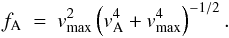 (2)For a typical coronal loop with a number density of 109 cm-3 and a magnetic field strength of 50 G at its apex, the Alfvén speed (≈ 3000 km s-1) is reduced by about a factor of 1.5. Significant corrections mostly occur in low-density regions (where the coronal Alfvén speed gets large), which does not appear bright in the synthetic images, and thus can be expected only to play a minor role for the analysis we present. Despite this limiting of the Alfvén speed, in the model corona the plasma-β is still well below 1 and the effective Alfvén speed is still an order of magnitude larger than the maximum sound speed (250 km s-1 at 3 MK). In summary, this limiting of the Alfvén speed only has a minor effect on our results, but it provides a significant speed-up of the numerical simulation.
Together, the treatment of the heat conduction and the Alfvén speed, only introduced to speed-up the simulation time, provide a speed-up of typically a factor of five, at little extra computational cost.
Our high-resolution simulation is able to resolve small-scale photospheric magnetic structures and flows related to the granular motions in the photosphere, which are used as input from the flux-emergence simulation. The interaction of the plasma flow and magnetic field in the model photosphere, especially at the outer edge of strong flux concentrations, produces the enhanced upward Poynting flux that can bring enough energy into the upper solar atmosphere and power the coronal loops. This energy flux sustains a more than 3 MK hot corona at pressures, according to the classical scaling laws (Rosner et al. 1978).
We show in Fig. 1 a snapshot of a time series of the synthesised EUV images according to the response function of the 211 Å channel of the Atmospheric Imaging Assembly (AIA, Boerner et al. 2012). Here we follow the procedure outlined in (Peter & Bingert 2012) to calculate the AIA emission expected from the model corona. In these synthetic images we find numerous bright EUV loops, which represent the coronal plasma at temperatures around 2 MK. In these loops the number density is about 109 cm-3. The properties of the coronal plasma are in quantitative agreement with our previous simulation, and they are also consistent with typical values derived from real observations.
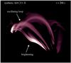 |
Fig. 1 System of coronal loops synthesised from 3D MHD model. This shows a snapshot of the model corona as it would appear in an EUV image taken by AIA in the 211 Å channel (in logarithmic scale). It is dominated by emission from Fe xiii showing plasma at around 2 MK. The distance between the two footpoints of the loop system is about 35 Mm and the loops have lengths of about 45 Mm to 50 Mm. The arrows indicate the position of the brightening, which triggers the oscillation (see Sect. 3.1) and oscillating loop (Sect. 3.3). The full temporal evolution over 54 min is available as a movie in the online edition. The movie starts early in the simulation when there is no coronal emission. In response to the flux emergence, coronal loops form and, at about 72.5 min, a trigger sets the oscillation in motion. Then, a second counter in the movie shows the time in starting at 72.5 min, consistent with the time used in Fig. 3. |
Beyond the appearance in a synthetic EUV snapshot, the model also captures the dynamic nature of the real corona to some extent. The animation associated with Fig. 1 shows that bright features can show up or disappear within a few minutes in a certain EUV passband. This is consistent with modern observations, for example from AIA.
3. Oscillation observed in synthesised coronal emission
3.1. Trigger of the oscillation
As in our previous model of an emerging active region (Chen et al. 2014, 2015), loops form in the active region in response to the heating driven by footpoint motions in the photosphere. This leads to a more or less continuous evolution of the loops: some loops form, others fade away. A snapshot of the loops in coronal emission is shown in Fig. 1, the temporal evolution is shown in the attached movie. In the following, we relate all times relative to the time 72.5 min after the actual start of the simulation.
At the time t ≈ 200 s, some loops start to oscillate just after a strong transient brightening of some close-by loops. These locations are indicated in the snapshot in Fig. 1 as well as in the attached movie.
We traced the cause of the strong transient brightening as being due to an enhancement of Ohmic heating along the field lines at the flank of the active region. The cool plasma is quickly heated to a temperature at which the response function of the AIA 211 Å channel peaks. The increase of the heating is caused by an increase of the currents in response to a reconfiguration of the coronal magnetic field driven by photospheric flows in the periphery of the sunspots (as the result of the flux emergence). The strong brightening associated with this increased heating rate can be considered a very small flare on the Sun (even though we do not imply here that this is a flare model).
The increased currents come along with a transient increase of the Lorentz force, leading to a kick that is perpendicular to the field lines. The disturbance propagates from the brightening site across the active region and triggers the transverse oscillation of the nearby loops. Again, this can be considered in analogy to eruptions on the real Sun, which are suggested to be the main trigger mechanism of observed loop oscillations. This oscillation is clear, albeit not violent, in the movie attached to Fig. 1.
The travel time of the triggering disturbance from the transient brightening to the farthest visible loop is about 12 s (propagation with an Alfvén speed of almost 2000 km s-1 across a distance of some 25 Mm). This is why at the cadence of 10 s, for the movie shown with Fig. 1, the oscillation of the loop seems to start at almost the same time as the transient brightening triggering the event.
The actual process triggering the oscillation is a very interesting process in itself, but it is not the main interest of this study. In contrast, we concentrate here on the observable consequences of this event and investigate to what extent the methods of coronal seismology can recover the atmospheric conditions at the location of the oscillating loop, in particular, the magnetic field.
3.2. Imaging and spectroscopy of model data
The synthesised imaging data (movie with Fig. 1) reveal a transverse oscillation in the loop, which lasts for about 300 s and gradually decays. Its appearance is similar to the oscillations widely found in EUV observations. Mostly this type of oscillation is interpreted as the standing, fast kink mode (e.g. Nakariakov & Verwichte 2005). Although the loop oscillation is clear in the animation for the human observer, a quantitative analysis of this oscillatory displacement of the loop position is not so clear because the amplitude of the oscillation is only of the order of or even smaller than the width of the coronal loop.
Alternatively, one can investigate the velocity disturbances through Doppler shifts from (synthesised) spectroscopic observations. Because the loops are inclined, when observed from straight above the transversely oscillating loops result in periodic Doppler shifts. To study this, we simulate an observation from the top of the active region, i.e. as if we would observe an active region at the disk centre. To this end, we calculate the emission line profile at each grid point based on the output of the MHD simulation and then integrate along a vertical line of sight. This procedure follows Peter et al. (2004, 2006). To be consistent with the imaging data shown in Fig. 1, we study line profiles from the same ion and choose the Fe xiii line at 202 Å line, which has been observed abundantly with the EUV Imaging Spectrometer (EIS; Culhane et al. 2007).
The Fe xiii profiles are mostly close to a single Gaussian. Their width is determined by the local plasma temperature and the distribution of the line-of-sight velocities. To derive the line intensity and shift we take the zeroth and first moment of the line profile. The resulting Doppler map in Fig. 2 basically shows the vertical (line-of-sight) velocity of the 2 MK hot plasma in the active region (at the same time as the snapshot in Fig. 1). This Doppler map shows the line shifts at the same time across the whole map. In a real observation with a slit spectrometer, one would have to produce a raster scan to obtain this map, e.g. EIS would need up to one hour to raster a field of view as shown in Fig. 2 (depending on observation parameters). Thus a real observation would look quite different from this instantaneous Doppler map.
In a real observation usually one would perform a so-called sit-and-stare observation to catch the oscillation, i.e. one would keep the slit at a fixed position in the active region and study the temporal evolution at that location. For our synthetic observations, we choose a slit oriented along the y-direction located directly in the middle between the footpoints of the loop (solid line in Fig. 2). The dotted line indicates the location of the loop that is seen to be oscillating in the intensity data (cf. movie with Fig. 1). Here we catch the loop in a phase of the oscillation moving away from the virtual observer. The slit roughly crosses the apex of the loops.
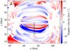 |
Fig. 2 Map of Doppler shifts of synthesised Fe xiii 202 Å data. This shows the active region seen from straight above, i.e. the line of sight is vertical, corresponding to an observation at disk centre. The black solid line indicates the position of the slit used to simulate a sit-and-stare observation for the analysis of the Doppler oscillation (see Fig. 3 and Sect. 3.2). The dotted line indicates the location of the oscillating loop, as seen in the movie attached to Fig. 1. |
For the further analysis, we extract the line intensity and the Doppler shift along this slit from the synthesised spectral data with a cadence of 10 s. This roughly matches the typical cadence used in real observations. The resulting time series of this synthetic observation is comparable to real data acquired from active region loops in a sit-and-stare observation.
3.3. Quantitative analysis of the loop oscillation
To analyse the oscillation we first check time-space diagrams for the line intensity and Doppler shift. As for sit-and-stare observations of the real Sun (e.g. Wang et al. 2009; Mariska & Muglach 2010), these show the line intensity and shift as a function of time and space (along the slit). For the slit position indicated in Fig. 2 these are shown in panels (a) and (b) of Fig. 3.
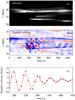 |
Fig. 3 Oscillation of the loop. Panels a) and b) show the intensity and Doppler shift of the Fe xiii line synthesised from the coronal model as a function of time and space along the slit. The location of the slit is indicated in Fig. 2 and the range of Doppler shifts is from −15 km s-1 to + 15 km s-1, just as in Fig. 2. The black boxes in these space-time plots indicate the position of the loop with the clearest oscillation pattern. Panel c) shows the Doppler shift of the loop as a function of time. Here the Doppler shifts are averaged along the slit across the loop, i.e. along y within the black box in panel b). The red line shows the fit by a damped sinusoidal function as defined in Eq. (3). See Sect. 3.3. |
The line intensity does not show a clear oscillation in the y-direction in this diagram. This is consistent with the impression from the synthetic AIA images that the amplitude of the oscillation (in space) is smaller than the loop width. In addition, the loop is inclined and the oscillation is transverse, which further reduces the amplitude of loop displacement.
In contrast, the oscillation is very clear in Doppler shift (Fig. 3b). It starts at around t = 200 s, which is consistent with the oscillation seen as a slight displacement of the loop in coronal emission (see movie with Fig. 1). The oscillatory pattern is seen over the whole field of view shown in Fig. 3b, underlining the impression from the intensity images that the trigger leads to a disturbance of a whole arcade of loops. While three distinct loops can be identified in Fig. 3a near y = 23′′, 26′′, and 29′′, in the following we concentrate on the latter. This shows the clearest oscillating pattern, which lasts from ca. t = 180 s to 450 s and is marked by a black box in Figs. 3a, b.
To obtain a clear signal, we average the Doppler shift in the oscillating loop in the black box in Fig. 3b in the y-direction. The resulting (mean) Doppler velocity as a function of time is shown by the black symbols in Fig. 3c, which clearly shows a damped oscillation. To extract the period P of the oscillation and its damping time τ, we fit this oscillation by an exponentially damped sinusoidal function, ![Mathematical equation: \begin{eqnarray} \label{E:osci} f(t)~~=~~A_0~\exp {\bigg[}{-}\frac{t-t_0}{\tau}{\bigg]} ~ \sin{\bigg[}\frac{2\pi}{P}(t-t_0){\bigg]} + A_1 t +A_2. \end{eqnarray}](/articles/aa/full_html/2015/09/aa26237-15/aa26237-15-eq26.png) (3)Here t is the time, t0 the initial time, and A0 the amplitude of the exponentially damped sinusoidal function. In addition, A1 and A2 account for a linear background. Fitting the Doppler shifts in Fig. 3c with a uniform weight, we obtain a period and a damping time of
(3)Here t is the time, t0 the initial time, and A0 the amplitude of the exponentially damped sinusoidal function. In addition, A1 and A2 account for a linear background. Fitting the Doppler shifts in Fig. 3c with a uniform weight, we obtain a period and a damping time of 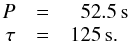 (4)We also applied the same analysis for some other slit positions. When the slit is located midway from the loop footpoint to the apex, the average Doppler perturbation in the loop appears very similar to that at the apex, albeit with a reduced amplitude. Still, the damping time and period derived at these other positions are fully consistent with the results at the loop apex. If the slit is positioned close to the loop footpoints, the oscillatory Doppler signal gets mixed with slowly changing Doppler shifts due to flows (along the magnetic field) filling and draining the loop (cf. Chen et al. 2014). Therefore, when analysing the oscillation close to the footpoints we first remove this smoothly varying signal before fitting the oscillation with Eq. (3). Again the period and damping time are consistent with the values found near the apex listed in Eq. (4). This underlines that the loop shows a coherent oscillation all along (see also Sect. 3.4).
Comparing these values of Eq. (4) to observations, they are found at the lower end of the distribution found in the compilation of oscillations by Verwichte et al. (2013b). This is not surprising because the size of our computational box is limited, and thus the loops we can study have lengths of below 50 Mm. The observed loops are mostly longer by a factor of two (or more). Hence the expected period would be longer by that factor (the period is proportional to the loop length, see Sect. 4.1.
An important observational test for our model loop is the scaling between period and damping time as derived by Verwichte et al. (2013b) based on a sample of 52 oscillating loops. They found τ = αPγ, with log10α = 0.44 ± 0.31 and γ = 0.94 ± 0.12. The period and damping time of the oscillation found in our model listed in Eq. (4) fits this scaling relation very well. This suggests that our model for the loop oscillation and its damping capture the right physical processes, even though the period and damping time are at the lower end of what is found in observations.
3.4. Mode of the oscillation
Apart from the measurement of the oscillation parameters, the identification of the corresponding wave mode is equally important. In the synthetic EUV images the loop oscillates primarily in the transverse direction without any visible (stationary) node along the loop (cf. movie with Fig. 1). This is supported by the Doppler patterns that have the same sign all along the loop (see Fig. 2). Together this suggests that the oscillation in the model is a fundamental kink mode.
A quantitative test for the presence of the fundamental kink mode is given through the phase difference of the velocity disturbance measured at different positions along the loop (D. Yuan, priv. comm.). Because the loop should oscillate coherently all along in the fundamental kink mode, this phase difference should vanish.
To estimate the phase difference between the velocity disturbance at different positions along the loop, we cross correlate the oscillation at the apex to four other locations, two midway to the footpoints, and two close to the footpoints at each side. To accomplish this, we use the fits to the variation of the Doppler shifts from Eq. (3) and show the cross correlation as a function of the time lag in Fig. 4. All cross correlations peak at about zero time lag, i.e. the velocity disturbances of the oscillation at different positions have no phase difference2. Moreover, the peak values of the cross correlations are close to unity, indicating that the oscillations are very similar at different positions, i.e. that the loop oscillates as a whole.
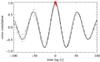 |
Fig. 4 Cross correlations of the oscillation at different locations along the loop. The five curves show the cross correlation of the loop apex with five positions along the loop (apex, two positions midway from apex to loop, and two near the footpoint at both sides). The solid line shows the self-correlation at the loop apex. The range of the time lag shown here is about four times the oscillation period of 52.5 s at the loop apex. The red diamonds indicate the peaks of the cross-correlation functions. See Sect. 3.4. |
Another indicator for the fundamental mode is given thorough the variation of the normal velocity along the loop. Because for the fundamental mode two nodes of the oscillation should be found at the footpoints, there should be a smooth drop of the normal velocity from the apex to the feet. This is confirmed by the plot in Fig. 5, which shows the normal velocity at a time near maximum velocity. There we also illustrate the difficulties that would be encountered in real solar observations for this test. While we have direct access to the normal velocity in our model, this is not the case in observations. To show this, in Fig. 5 we also plot the Doppler shift as it changes along the loop when observing from straight above (i.e. the shift along the dotted line in Fig. 2). Essentially this shows the vertical velocity in the loop. While this basically reflects the line-of-sight component of the normal velocity near the apex, this signal is heavily contaminated by the flows in or out of the loop near the footpoints. Here we see a draining of the loop, i.e. downflows at both footpoints. The downflows (12 km s-1 and 24 km s-1) are comparable with the transverse oscillation speed (14 km s-1) at the loop apex. This might prevent any solid conclusions in real observations regarding the wave mode via measurements of the Doppler shift variation along the loop.
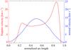 |
Fig. 5 Line-of-sight Doppler shift and normal velocity of the oscillation along the loop. The blue curve shows the velocity of the oscillating loop in the normal direction at a snapshot of maximum velocity amplitude (at t = 200 s). The red line indicates the Doppler shifts from the synthesised spectral profiles, basically the vertical velocity in the loop, which also show signs of the field-aligned flows near the footpoints. The arc length has been normalised to the loop length, i.e. the footpoints in the photosphere are at 0 and 1, and the apex is around 0.5. See Sect. 3.4. |
This result also illustrates an important constraint on simplified models for loop oscillations. Because one never prevents these in- or outflows near the loop footpoints in a model that is complex enough (we never see static loops in the 3D models) or on the real Sun, we have to take these flow structures into account, in particular, because these flow speeds reach a good fraction of the sound speed.
Together with the fact that the same periods and damping times are found all along the loop (Sect. 3.3), the zero time-lag of the oscillation at different places along the loop and the clear existence of nodes at the footpoints underlines that the oscillation in our model loop is indeed a fundamental kink mode.
4. Oscillation frequency and magnetic field
4.1. Estimate of the magnetic field strength from coronal seismology
In a seminal paper, Edwin & Roberts (1983) showed that the period of a loop oscillating in the corona would depend on the magnetic field, which in turn enables the estimation of the field strength if one can identify the oscillation and determine its frequency. In an observation, the phase speed ck of a kink mode oscillation is usually estimated with  (5)where L is the loop length and P the oscillation period (e.g. Nakariakov et al. 1999). The loop length is determined from EUV imaging observations and the period by fitting the oscillation in the displacement of the loop position of the Doppler shift (e.g. as described in Sect. 3.3). Table 1 summarises these parameters derived from our synthesised observation of the oscillating loop and other loop parameters and results. The value we derive here for ck of 1730 km s-1 is still below the limiting Alfvén speed for the simulation, see discussion with Eq. (1). When we derive the magnetic field strength, we still consider the limiting in the analysis below in Eq. (7).
Parameters of the oscillating loop.
As derived by Edwin & Roberts (1983), the phase speed of this kink mode in a slender magnetic flux tube with uniform density depends on the Alfvén speed vA and the density ρ inside and outside the flux tube,  (6)Here the subscripts i and e refer to internal and external, i.e. to inside and outside the flux tube.
Because the corona is a low-β plasma, it is usually assumed that the magnetic field strength Bkink (derived from the kink mode oscillation) inside and outside the loop is the same. In our MHD simulation, we can confirm that this is indeed the case. Using the effective Alfvén speed in our model from Eq. (1) to account for the Alfvén speed limiting, Eq. (6) reads ![Mathematical equation: \begin{eqnarray} \label{E:ck2} c_{\rm k}~~=~~\frac{B_{\rm{kink}}}{~\sqrt{\mu_0\rho_{\rm i}}~}~~\left(\frac{2}{1+\rho_{\rm e}/\rho_{\rm i}}\right)^{\!\!1/2}~~\left[\frac{f_{\rm Ai}+f_{\rm Ae}}{2}\right]^{\!1/2}\cdot \end{eqnarray}](/articles/aa/full_html/2015/09/aa26237-15/aa26237-15-eq52.png) (7)The last term [···] is not present when observers analyse their data. It is an artifact of the Alfvén speed limiting we applied in our model (see Sect. 2) and consequently we have to correct for this here as well.
(7)The last term [···] is not present when observers analyse their data. It is an artifact of the Alfvén speed limiting we applied in our model (see Sect. 2) and consequently we have to correct for this here as well.
If observations provided the kink mode wave speed through Eq. (5) and if the internal and external densities can also be estimated from observations, then Eq. (7) provides an estimate for the magnetic field strength in the loop based on the analysis of the kink mode, Bkink. In absence of a reliable tool for density diagnostics when using imaging observations, one often simply assumes a typical value for the coronal density, e.g. 109 cm-3, and a typical density contrast of ρe/ρi = 0.1.
We use the values for the internal and external densities as derived directly from the MHD model (see Table 1). To accomplish this, we choose a group of magnetic field lines within the cross section of the oscillating loop as seen in EUV emission for the internal properties and another group of magnetic field lines in the ambient corona outside for the external properties. In Fig. 6a we plot the number density and temperature averaged for the respective group of field lines along the loop, separately for the conditions inside and outside the loop.
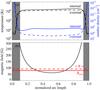 |
Fig. 6 Plasma parameters and magnetic field strength along the loop. Panel a) shows the temperature (black) and density (blue) for the condition inside the EUV loop (solid lines labelled internal). The corresponding values just outside the loop are plotted as dashed lines (labelled external). Panel b) shows the magnetic field strength along the loop in the 3D MHD model. The red solid line shows the coronal magnetic field strength derived from the kink oscillation, Bkink, and the red dashed line indicates the average magnetic field strength, ⟨ B ⟩, defined by Eq. (8). The position along the loop is normalised by the total loop length (53 Mm). The positions 0.0 and 1.0 are at footpoints in the photosphere. The grey areas indicate the lower atmosphere, where T< 1 MK. The loop length in the coronal part, i.e. between the grey regions, is about 45 Mm. See Sect. 3.3 for panel a) and Sects. 4.1 and 4.2 for panel b). |
In the coronal part (i.e. where T> 106 K) of the EUV loop, as well of the flux tube just outside the loop, the temperature and density are roughly constant. This is because of the highly efficient heat conduction and large pressure scale height at high temperatures. In this coronal part (between the grey hatched areas of Fig. 6), the average density inside the EUV loop is about ρi = 3.8 × 10⁻¹² kg m-3 (ni = 5.7 × 108 cm-3). Outside the loop, the external average density is ρe = 4.4 × 10⁻¹³ kg m-3 (ne = 6.5 × 107 cm-3). The resulting density ratio is about ρe/ρi = 0.12. The density we find in the loop is comparable to typically assumed values, and also the ratio is similar to the typical assumptions applied for tube models and for the inversion of observations (e.g. ρe/ρi = 0.1 by Nakariakov & Ofman 2001).
The loop length in the coronal part is roughly 45 Mm, which is consistent with the length one would derive from the synthesised EUV images. Together with the oscillation period of P = 52.5 s derived from fitting the oscillation in Sect. 3.3, we obtain a kink-mode phase speed of ck = 1730 km s-1 from Eq. (5). With the densities derived above, we can use the value of ck to derive the coronal magnetic field strength, based on the kink mode oscillation from Eq. (7), which yields Bkink = 79 G.
This derivation of the average coronal magnetic field strength basically copies the procedure applied to observations. Now the main question is what this average actually means.
4.2. Comparison with the actual magnetic field strength along the loop
The magnetic field strength varies along the coronal loop in both the real corona and our numerical model, basically reflecting the expansion of the magnetic field. Therefore, the value deduced from coronal seismology does not necessarily represent the field strength at any particular position of the loop, but is an average through the coronal part of the loop. Most importantly, the significant variation of the magnetic field along the loop is usually neglected in coronal seismology, even though the importance of this effect has been shown before (e.g. Ofman et al. 2012). The profile of the magnetic field strength along the loop in our model (along the centre field line of the loop) is plotted in Fig. 6b. In the following, we investigate the field strength (e.g. its average) in the coronal part only, i.e. where T> 106 K between the grey areas in Fig. 6.
The arithmetic mean of the magnetic field strength along the loop is 120 G, i.e. significantly higher than the value of Bkink = 79 G derived from the oscillation. The reason for this discrepancy is that coronal seismology estimates the magnetic field strength from the observed average wave speed as defined as Eq. (5). Because the actual wave speed is (usually) not constant through the loop, this gives more weight to regions of low Alfvén speeds, i.e. to regions where the propagating wave packet dwells the longest. These are the regions of low magnetic field strength, which is why the magnetic field strength derived from oscillations is much lower than an arithmetic mean.
To define an average that is closer to the value derived from oscillations, one has to account for the variation of the wave speed (or in other words, the wave travel time). Following Aschwanden & Schrijver (2011), we define ![Mathematical equation: \begin{eqnarray} \label{E:B_ave} \left\langle B \right\rangle~=~L\,\left[\int \frac{{\rm d}s}{B(s)}\right]^{-1}, \end{eqnarray}](/articles/aa/full_html/2015/09/aa26237-15/aa26237-15-eq68.png) (8)where s is the coordinate along the arc length of the loop. Aschwanden & Schrijver (2011) argue that a flux tube with a field strength B(s) changing along the loop would oscillate with the same frequency as a flux tube with a constant field strength ⟨ B ⟩ as derived from Eq. (8). In our model loop, we find ⟨ B ⟩ = 92 G, as indicated by the red dashed line in Fig. 6b. Compared with the arithmetic average along the loop, this is closer to the magnetic field derived from the kink mode, Bkink = 79 G, but it is still significantly larger by some 15% to 20%.
(8)where s is the coordinate along the arc length of the loop. Aschwanden & Schrijver (2011) argue that a flux tube with a field strength B(s) changing along the loop would oscillate with the same frequency as a flux tube with a constant field strength ⟨ B ⟩ as derived from Eq. (8). In our model loop, we find ⟨ B ⟩ = 92 G, as indicated by the red dashed line in Fig. 6b. Compared with the arithmetic average along the loop, this is closer to the magnetic field derived from the kink mode, Bkink = 79 G, but it is still significantly larger by some 15% to 20%.
The fact that the average ⟨ B ⟩ based on Eq. (8) comes reasonably close to the value derived from the oscillation, Bkink, underlines that the magnetic field strength estimated by coronal seismology represents the average magnetic field weighted with the wave speed along the loop. Basically coronal seismology returns the value of the magnetic field that one would find in a flux tube with a constant magnetic field with the same Alfvén crossing time.
However, the field derived by coronal seismology, Bkink, is still 15% to 20% smaller than the average ⟨B⟩, i.e. the true magnetic field in our simulation (or on the real Sun). This implies that the actual wave speed (in the model) is underestimated by the theoretical value from coronal seismology. A difference of up to 50% between the derived magnetic field strength and the actual field strength was also found by De Moortel & Pascoe (2009) who investigated a MHD model (albeit with a less realistic magnetic set-up and much simpler thermodynamics). They concluded that this is because “the combined effect of the loop curvature, the density ratio, and aspect ratio of the loop appears to be more important than previously expected” (De Moortel & Pascoe 2009).
Furthermore, the (magnetic) complexity of coronal loops in our model and on the real Sun could lead to this kind of deviation. One possible explanation might be the aspect ratio (i.e. width/length) of the loop. The particular oscillating loop highlighted in Fig. 1 has an aspect ratio of about 0.04 (2 Mm width, 45 Mm long; other loops in the model are thinner). The aspect ratio is a bit smaller in observations, typically 0.02 (2 Mm width at 100 Mm length). However, it has to be noted that here the width refers to the width of the EUV loop, while 3D models show that these EUV loops are embedded in thicker corresponding density structures (Peter & Bingert 2012; Chen et al. 2014). Thus we can expect the aspect ratio to be several percent.
Edwin & Roberts (1983) noted that the actual kink mode speed is only equal to ck defined by Eq. (6) if the width of the flux tube is much smaller than the wavelength of the disturbance. Otherwise, it decreases with an increasing aspect ratio (see Eq. (15) in Edwin & Roberts 1983). Therefore it might be that in our model (and on the real Sun) this assumption of Edwin & Roberts (1983) is not fully applicable. Other effects, e.g. that plasma-β is non-zero (see Eq. (11) for large β of Edwin & Roberts 1983), a smooth density profile across the loop, or flows along the loop might also play a role in our model as well as on the real Sun. A detailed theoretical investigation of these effects is beyond the scope of this paper, but should be addressed in a future study.
5. Damping of the oscillation and Reynolds number
So far we concentrated on the frequency of the loop oscillation to investigate the magnetic field strength in the loop. We now turn to the damping time τ of the oscillation as defined through Eq. (3) and discuss consequences for the dissipation and thus for the (magnetic) Reynolds number.
Damping is commonly found in transverse loop oscillations. The damping time is particularly important because it reflects the rate at which the wave energy is either converted into another wave mode or dissipated. Using a scaling relation derived from numerical models, Nakariakov et al. (1999) found that the magnetic Reynolds number deduced from the observed damping time is of the order of 106. This is several orders of magnitude smaller than the classical value that would be of the order of 1014, and consequently would indicate an anomalously high dissipation. Later, Ofman & Aschwanden (2002) quantified this further through an analysis of the scaling relation between damping time and loop parameters. They estimated an anomalously large viscosity of 109.2 ± 3.5 m2 s-1, which also gives a Reynolds number that is much smaller than the classical value. These results imply that the wave energy could be efficiently converted into heat because of the anomalously high diffusivity. Still, one has to keep in mind that the damping is not necessarily due to dissipation of the wave energy (even though ultimately the wave is dissipated). Goossens et al. (2002) argued that the observed fast damping of transverse loop oscillations can be explained by the damping of quasi-mode kink oscillations. Thus, they suggested that there might be no need for the anomalously large viscosity.
In our model the magnetic resistivity η is 5 × 10⁹ m2 s-1 (and the kinematic viscosity ν is of the same order). Essentially this value is determined by the grid spacing in the numerical models (Bingert & Peter 2011; Peter 2015) and ensures that currents that build up because of the driving of the magnetic field by photospheric motions is dissipated at scales of the grid spacing. These values of resistivity and viscosity are in the middle of the range of values found by Ofman & Aschwanden (2002), i.e. 109.2 ± 3.5 m2 s-1. From this, we conclude that the dissipation coefficient in our model (109.7 m2 s-1) is consistent with the high values found in observations.
If we take the loop half width of our model loop (≈ 1 Mm) as a length scale, the dissipation time for the wave in our model would be τdiss ≈ (1 Mm)2/ 5 × 10⁹ m2 s-1 = 200 s, which is close to the damping time of 125 s for the oscillation in our model. This suggests that in our model the damping is indeed due to (resistive and viscous) dissipation. A more detailed analysis of the energy budget will be needed to investigate how much of the energy released by the trigger is first converted into the oscillation and then dissipated by viscosity and resistivity. In particular, further investigations will be needed to study the role of the spatial resolution and thus of the Reynolds number on the resulting oscillations.
6. Conclusions
We presented a loop oscillation found in a realistic coronal model driven by magnetic flux emergence through the photosphere (i.e. the bottom boundary). The treatment of the energy balance in the model allows us to synthesise imaging and spectroscopic observations from the model. There we found a clear transverse loop oscillation, which we identified as the fundamental fast kink mode. The period (P = 52.5 s) and damping time (τ = 125 s) of the oscillation are consistent with observations. In particular, our oscillation also follows the observed relation between period and damping time deduced by Verwichte et al. (2013b). At least in our model the damping of the oscillation is due to resistive and viscous dissipation. To what extent this conclusion can also be drawn for the real Sun will have to be revealed by new simulations at higher spatial resolution.
We applied methods of coronal seismology to the coronal emission synthesised from our model corona as would be done for real observations. Here we concentrated on the oscillation in the Doppler shift of a coronal emission line. We chose a (vertical) line of sight for the analysis of the model data that mimics the observation of a coronal loop near disk centre.
Based on the fundamental kink mode oscillation, we deduced an average magnetic field strength of Bkink = 79 G in the loop. In contrast to solar observations, in the model we know the magnetic field in the oscillating loop. This way we can understand what the field strength derived from coronal seismology actually means. In the coronal part of the model loop the magnetic field strength varies strongly by about a factor of five and drops to some 50 G near the apex, i.e. significantly below the value derived from coronal seismology, Bkink. The average of the field along the loops, as suggested by Aschwanden & Schrijver (2011), gives a relatively good match, ⟨ B ⟩ = 92 G. This average of the field corresponds to the constant field in a flux tube with a constant cross section that has the same wave travel time. Still, the difference between Bkink and ⟨ B ⟩ is considerable. Because many of the assumptions of the simple derivation of the wave period are violated in the model (and most certainly on the real Sun), e.g. the loop width, substructure, or dynamics, this is not too surprising.
We conclude that the magnetic field strength deduced by coronal seismology can be a good representative of that in the upper part of coronal loop. Realistic models like the one presented here might further guide the interpretation of coronal oscillation results, in particular, might relax some of the assumptions to get a better match to coronal properties derived from coronal seismology.
Online material
Movie of Fig. 1 Access Supplementary Material
See also http://pencil-code.nordita.org
For kink mode oscillations, there is a phase difference of π/ 2 between the velocity disturbance and the displacement at the same position of the loop.
Acknowledgments
The authors thank Ding Yuan, Tom van Doorsselaere, and Leon Ofman for helpful suggestions. F.C. thanks Rony Keppens for supporting his visit to Katholieke Universiteit Leuven. The authors also thank Sven Bingert for help in setting up the simulation, and Mark Cheung for offering the data that are used as the bottom boundary of the simulation. This work was supported by the International Max-Planck Research School (IMPRS) for Solar System Science at the University of Göttingen. We acknowledge PRACE for awarding us the access to SuperMUC based in Germany at the Leibniz Supercomputing Centre (LRZ).
References
- Arregui, I., Terradas, J., Oliver, R., & Ballester, J. L. 2007, A&A, 466, 1145 [NASA ADS] [CrossRef] [EDP Sciences] [Google Scholar]
- Aschwanden, M. J., Fletcher, L., Schrijver, C. J., & Alexander, D. 1999, ApJ, 520, 880 [NASA ADS] [CrossRef] [Google Scholar]
- Aschwanden, M. J., & Schrijver, C. J. 2011, ApJ, 736, 102 [NASA ADS] [CrossRef] [Google Scholar]
- Banerjee, D., Erdélyi, R., Oliver, R., & O’Shea, E. 2007, Sol. Phys., 246, 3 [NASA ADS] [CrossRef] [Google Scholar]
- Bingert, S., & Peter, H. 2011, A&A, 530, A112 [NASA ADS] [CrossRef] [EDP Sciences] [Google Scholar]
- Bingert, S., & Peter, H. 2013, A&A, 550, A30 [NASA ADS] [CrossRef] [EDP Sciences] [Google Scholar]
- Boerner, P., Edwards, C., Lemen, J., et al. 2012, Sol. Phys., 275, 41 [NASA ADS] [CrossRef] [Google Scholar]
- Bourdin, P.-A., Bingert, S., & Peter, H. 2013, A&A, 555, A123 [NASA ADS] [CrossRef] [EDP Sciences] [Google Scholar]
- Brandenburg, A., & Dobler, W. 2002, Comp. Phys. Comm., 147, 471 [Google Scholar]
- Chen, F., Peter, H., Bingert, S., & Cheung, M. C. M. 2014, A&A, 564, A12 [NASA ADS] [CrossRef] [EDP Sciences] [Google Scholar]
- Chen, F., Peter, H., Bingert, S., & Cheung, M. C. M. 2015, Nature Phys., 11, 492 [Google Scholar]
- Cheung, M. C. M., Rempel, M., Title, A. M., & Schüssler, M. 2010, ApJ, 720, 233 [NASA ADS] [CrossRef] [Google Scholar]
- Culhane, J. L., Harra, L. K., James, A. M., et al. 2007, Sol. Phys., 243, 19 [Google Scholar]
- De Moortel, I., & Nakariakov, V. M. 2012, Roy. Soc. London Philos. Trans. Ser. A, 370, 3193 [Google Scholar]
- De Moortel, I., & Pascoe, D. J. 2009, ApJ, 699, L72 [NASA ADS] [CrossRef] [Google Scholar]
- De Moortel, I., Ireland, J., & Walsh, R. W. 2000, A&A, 355, L23 [NASA ADS] [Google Scholar]
- Edwin, P. M., & Roberts, B. 1983, Sol. Phys., 88, 179 [NASA ADS] [CrossRef] [Google Scholar]
- Erdélyi, R., & Taroyan, Y. 2008, A&A, 489, L49 [NASA ADS] [CrossRef] [EDP Sciences] [Google Scholar]
- Erdélyi, R., & Verth, G. 2007, A&A, 462, 743 [NASA ADS] [CrossRef] [EDP Sciences] [Google Scholar]
- Feng, L., Inhester, B., Solanki, S. K., et al. 2007, ApJ, 671, L205 [NASA ADS] [CrossRef] [Google Scholar]
- Goossens, M., Andries, J., & Aschwanden, M. J. 2002, A&A, 394, L39 [NASA ADS] [CrossRef] [EDP Sciences] [Google Scholar]
- Goossens, M., Terradas, J., Andries, J., Arregui, I., & Ballester, J. L. 2009, A&A, 503, 213 [NASA ADS] [CrossRef] [EDP Sciences] [Google Scholar]
- Gudiksen, B. V., & Nordlund, Å. 2005a, ApJ, 618, 1020 [NASA ADS] [CrossRef] [Google Scholar]
- Gudiksen, B. V., & Nordlund, Å. 2005b, ApJ, 618, 1031 [NASA ADS] [CrossRef] [Google Scholar]
- Guo, Y., Erdélyi, R., Srivastava, A. K., et al. 2015, ApJ, 799, 151 [NASA ADS] [CrossRef] [Google Scholar]
- Mariska, J. T. 1992, The solar transition region (New York: Cambridge University Press) [Google Scholar]
- Mariska, J. T., & Muglach, K. 2010, ApJ, 713, 573 [NASA ADS] [CrossRef] [Google Scholar]
- Meyer, C. D., Balsara, D. S., & Aslam, T. D. 2012, MNRAS, 422, 2102 [NASA ADS] [CrossRef] [Google Scholar]
- Nakariakov, V. M., & Ofman, L. 2001, A&A, 372, L53 [NASA ADS] [CrossRef] [EDP Sciences] [Google Scholar]
- Nakariakov, V. M., & Verwichte, E. 2005, Liv. Rev. Sol. Phys., 2, 3 [Google Scholar]
- Nakariakov, V. M., Ofman, L., Deluca, E. E., Roberts, B., & Davila, J. M. 1999, Science, 285, 862 [NASA ADS] [CrossRef] [PubMed] [Google Scholar]
- Ofman, L., & Aschwanden, M. J. 2002, ApJ, 576, L153 [NASA ADS] [CrossRef] [Google Scholar]
- Ofman, L., & Wang, T. 2002, ApJ, 580, L85 [NASA ADS] [CrossRef] [Google Scholar]
- Ofman, L., & Wang, T. J. 2008, A&A, 482, L9 [NASA ADS] [CrossRef] [EDP Sciences] [Google Scholar]
- Ofman, L., Wang, T. J., & Davila, J. M. 2012, ApJ, 754, 111 [NASA ADS] [CrossRef] [Google Scholar]
- Parker, E. N. 1972, ApJ, 174, 499 [NASA ADS] [CrossRef] [Google Scholar]
- Pascoe, D. J., de Moortel, I., & McLaughlin, J. A. 2009, A&A, 505, 319 [NASA ADS] [CrossRef] [EDP Sciences] [Google Scholar]
- Peter, H. 2015, Roy. Soc. London Philos. Trans. Ser. A, 373, 50055 [Google Scholar]
- Peter, H., & Bingert, S. 2012, A&A, 548, A1 [NASA ADS] [CrossRef] [EDP Sciences] [Google Scholar]
- Peter, H., Gudiksen, B. V., & Nordlund, Å. 2004, ApJ, 617, L85 [NASA ADS] [CrossRef] [Google Scholar]
- Peter, H., Gudiksen, B. V., & Nordlund, Å. 2006, ApJ, 638, 1086 [NASA ADS] [CrossRef] [MathSciNet] [Google Scholar]
- Priest, E. R., Heyvaerts, J. F., & Title, A. M. 2002, ApJ, 576, 533 [NASA ADS] [CrossRef] [Google Scholar]
- Rempel, M., & Cheung, M. C. M. 2014, ApJ, 785, 90 [Google Scholar]
- Rempel, M., Schüssler, M., & Knölker, M. 2009, ApJ, 691, 640 [NASA ADS] [CrossRef] [Google Scholar]
- Roberts, B., Edwin, P. M., & Benz, A. O. 1984, ApJ, 279, 857 [NASA ADS] [CrossRef] [Google Scholar]
- Rosner, R., Tucker, W. H., & Vaiana, G. S. 1978, ApJ, 220, 643 [NASA ADS] [CrossRef] [Google Scholar]
- Ruderman, M. S., & Erdélyi, R. 2009, Space Sci. Rev., 149, 199 [NASA ADS] [CrossRef] [Google Scholar]
- Schrijver, C. J., De Rosa, M. L., Metcalf, T. R., et al. 2006, Sol. Phys., 235, 161 [Google Scholar]
- Selwa, M., Ofman, L., & Solanki, S. K. 2011, ApJ, 726, 42 [NASA ADS] [CrossRef] [Google Scholar]
- Tian, H., McIntosh, S. W., Wang, T., et al. 2012, ApJ, 759, 144 [NASA ADS] [CrossRef] [Google Scholar]
- Uchida, Y. 1970, PASJ, 22, 341 [NASA ADS] [Google Scholar]
- Van Doorsselaere, T., Debosscher, A., Andries, J., & Poedts, S. 2004, A&A, 424, 1065 [NASA ADS] [CrossRef] [EDP Sciences] [Google Scholar]
- Van Doorsselaere, T., Nakariakov, V. M., Young, P. R., & Verwichte, E. 2008, A&A, 487, L17 [NASA ADS] [CrossRef] [EDP Sciences] [Google Scholar]
- Verwichte, E., Foullon, C., & Nakariakov, V. M. 2006, A&A, 452, 615 [NASA ADS] [CrossRef] [EDP Sciences] [Google Scholar]
- Verwichte, E., Van Doorsselaere, T., Foullon, C., & White, R. S. 2013a, ApJ, 767, 16 [NASA ADS] [CrossRef] [Google Scholar]
- Verwichte, E., Van Doorsselaere, T., White, R. S., & Antolin, P. 2013b, A&A, 552, A138 [NASA ADS] [CrossRef] [EDP Sciences] [Google Scholar]
- Wang, T. 2011, Space Sci. Rev., 158, 397 [NASA ADS] [CrossRef] [Google Scholar]
- Wang, T. J., Solanki, S. K., Curdt, W., et al. 2003, A&A, 406, 1105 [NASA ADS] [CrossRef] [EDP Sciences] [Google Scholar]
- Wang, T., Innes, D. E., & Qiu, J. 2007, ApJ, 656, 598 [NASA ADS] [CrossRef] [Google Scholar]
- Wang, T. J., Ofman, L., & Davila, J. M. 2009, ApJ, 696, 1448 [NASA ADS] [CrossRef] [Google Scholar]
- Wiegelmann, T., & Sakurai, T. 2012, Liv. Rev. Sol. Phys., 9, 5 [Google Scholar]
- Yuan, D., & Nakariakov, V. M. 2012, A&A, 543, A9 [NASA ADS] [CrossRef] [EDP Sciences] [Google Scholar]
All Tables
All Figures
|
Fig. 1 System of coronal loops synthesised from 3D MHD model. This shows a snapshot of the model corona as it would appear in an EUV image taken by AIA in the 211 Å channel (in logarithmic scale). It is dominated by emission from Fe xiii showing plasma at around 2 MK. The distance between the two footpoints of the loop system is about 35 Mm and the loops have lengths of about 45 Mm to 50 Mm. The arrows indicate the position of the brightening, which triggers the oscillation (see Sect. 3.1) and oscillating loop (Sect. 3.3). The full temporal evolution over 54 min is available as a movie in the online edition. The movie starts early in the simulation when there is no coronal emission. In response to the flux emergence, coronal loops form and, at about 72.5 min, a trigger sets the oscillation in motion. Then, a second counter in the movie shows the time in starting at 72.5 min, consistent with the time used in Fig. 3. |
| In the text | |
|
Fig. 2 Map of Doppler shifts of synthesised Fe xiii 202 Å data. This shows the active region seen from straight above, i.e. the line of sight is vertical, corresponding to an observation at disk centre. The black solid line indicates the position of the slit used to simulate a sit-and-stare observation for the analysis of the Doppler oscillation (see Fig. 3 and Sect. 3.2). The dotted line indicates the location of the oscillating loop, as seen in the movie attached to Fig. 1. |
| In the text | |
|
Fig. 3 Oscillation of the loop. Panels a) and b) show the intensity and Doppler shift of the Fe xiii line synthesised from the coronal model as a function of time and space along the slit. The location of the slit is indicated in Fig. 2 and the range of Doppler shifts is from −15 km s-1 to + 15 km s-1, just as in Fig. 2. The black boxes in these space-time plots indicate the position of the loop with the clearest oscillation pattern. Panel c) shows the Doppler shift of the loop as a function of time. Here the Doppler shifts are averaged along the slit across the loop, i.e. along y within the black box in panel b). The red line shows the fit by a damped sinusoidal function as defined in Eq. (3). See Sect. 3.3. |
| In the text | |
|
Fig. 4 Cross correlations of the oscillation at different locations along the loop. The five curves show the cross correlation of the loop apex with five positions along the loop (apex, two positions midway from apex to loop, and two near the footpoint at both sides). The solid line shows the self-correlation at the loop apex. The range of the time lag shown here is about four times the oscillation period of 52.5 s at the loop apex. The red diamonds indicate the peaks of the cross-correlation functions. See Sect. 3.4. |
| In the text | |
|
Fig. 5 Line-of-sight Doppler shift and normal velocity of the oscillation along the loop. The blue curve shows the velocity of the oscillating loop in the normal direction at a snapshot of maximum velocity amplitude (at t = 200 s). The red line indicates the Doppler shifts from the synthesised spectral profiles, basically the vertical velocity in the loop, which also show signs of the field-aligned flows near the footpoints. The arc length has been normalised to the loop length, i.e. the footpoints in the photosphere are at 0 and 1, and the apex is around 0.5. See Sect. 3.4. |
| In the text | |
|
Fig. 6 Plasma parameters and magnetic field strength along the loop. Panel a) shows the temperature (black) and density (blue) for the condition inside the EUV loop (solid lines labelled internal). The corresponding values just outside the loop are plotted as dashed lines (labelled external). Panel b) shows the magnetic field strength along the loop in the 3D MHD model. The red solid line shows the coronal magnetic field strength derived from the kink oscillation, Bkink, and the red dashed line indicates the average magnetic field strength, ⟨ B ⟩, defined by Eq. (8). The position along the loop is normalised by the total loop length (53 Mm). The positions 0.0 and 1.0 are at footpoints in the photosphere. The grey areas indicate the lower atmosphere, where T< 1 MK. The loop length in the coronal part, i.e. between the grey regions, is about 45 Mm. See Sect. 3.3 for panel a) and Sects. 4.1 and 4.2 for panel b). |
| In the text | |
Current usage metrics show cumulative count of Article Views (full-text article views including HTML views, PDF and ePub downloads, according to the available data) and Abstracts Views on Vision4Press platform.
Data correspond to usage on the plateform after 2015. The current usage metrics is available 48-96 hours after online publication and is updated daily on week days.
Initial download of the metrics may take a while.