| Issue |
A&A
Volume 580, August 2015
|
|
|---|---|---|
| Article Number | A82 | |
| Number of page(s) | 33 | |
| Section | Interstellar and circumstellar matter | |
| DOI | https://doi.org/10.1051/0004-6361/201525970 | |
| Published online | 06 August 2015 | |
Accretion dynamics of EX Lupi in quiescence
The star, the spot, and the accretion column⋆
1 School of Physics and Astronomy, University of St Andrews, North Haugh, St. Andrews KY16 9SS, UK
e-mail: This email address is being protected from spambots. You need JavaScript enabled to view it.
2 Departamento de Física Teórica, Facultad de Ciencias, Universidad Autónoma de Madrid, 28049 Cantoblanco, Madrid, Spain
3 Universitäts-Sternwarte München, Ludwig-Maximilians-Universität, Scheinerstr. 1, 81679 München, Germany
4 Konkoly Observatory, Research Center for Astronomy and Earth Sciences, Hungarian Academy of Sciences, PO Box 67, 1525 Budapest, Hungary
5 Max-Planck-Institut für Astronomie, Königstuhl 17, 69117 Heidelberg, Germany
6 Institute for Astronomy, ETH Zürich, Wolfgang-Pauli-Strasse 27, 8093 Zürich, Switzerland
Received: 26 February 2015
Accepted: 26 May 2015
Abstract
Context. EX Lupi is a young, accreting M0 star and the prototype of EXor variable stars. Its spectrum is very rich in emission lines, including many metallic lines with narrow and broad components. The presence of a close companion has also been proposed, based on radial velocity signatures.
Aims. We use the metallic emission lines to study the accretion structures and to test the companion hypothesis.
Methods. We analyse 54 spectra obtained during five years of quiescence time. We study the line profile variability and the radial velocity of the narrow and broad metallic emission lines. We use the velocity signatures of different species with various excitation conditions and their time dependency to track the dynamics associated with accretion.
Results. We observe periodic velocity variations in the broad and the narrow line components, consistent with rotational modulation. The modulation is stronger for lines with higher excitation potentials (e.g. He II), which are likely produced in a confined area very close to the accretion shock.
Conclusions. We propose that the narrow line components are produced in the post-shock region, while the broad components originate in the more extended, pre-shock material in the accretion column. All the emission lines suffer velocity modulation due to the rotation of the star. The broad components are responsible for the line-dependent veiling observed in EX Lupi. We demonstrate that a rotationally modulated line-dependent veiling can explain the radial velocity signature of the photospheric absorption lines, making the close-in companion hypothesis unnecessary. The accretion structure is locked to the star and very stable during the five years of observations. Not all stars with similar spectral types and accretion rates show the same metallic emission lines, which could be related to differences in temperature and density in their accretion structure(s). The contamination of photospheric signatures by accretion-related processes can be turned into a very useful tool for determining the innermost details of the accretion channels in the proximity of the star. The presence of emission lines from very stable accretion columns will nevertheless be a very strong limitation for the detection of companions by radial velocity in young stars, given the similarity of the accretion-related signatures with those produced by a companion.
Key words: stars: pre-main sequence / stars: variables: T Tauri, Herbig Ae/Be / stars: individual: EX Lupi / protoplanetary disks / accretion, accretion disks / techniques: spectroscopic
Appendices are available in electronic form at http://www.aanda.org
© ESO, 2015
1. Introduction
EX Lupi is the prototype of EXor variables and a remarkable object. Its strong variability episodes have been known for more than 50 years (McLaughlin 1946; Herbig 1950). The photospheric emission observed during the quiescent phases is compatible with a young star with spectral type M0 (Herbig 1977; Gras-Velázquez & Ray 2005). The star is known to have short-timescale, moderate (1−2 mag) variability (Herbig 1977; Lehman et al. 1995) caused by small variations in the accretion rate, together with rarer extreme variability episodes (increasing by 4−5 mag in the optical), of which only two have been documented to date: the first in the 1950s (Herbig 1977), and a second in 2008 (Jones 2008). In these extreme variability episodes, the accretion rate increased by more than two orders of magnitude during a few months time, before the star went back to quiescence (Ábrahám et al. 2009).
The main characteristic of the EX Lupi spectra is the large number of emission lines observed, both in quiescence and in outburst (Patten et al. 1994; Herbig et al. 2001; Sipos et al. 2009; Kóspál et al. 2008, 2011; Sicilia-Aguilar et al. 2012, hereafter SA12). During its strong 2008 outburst, the whole spectrum was dominated by emission lines and the stellar photosphere was completely veiled, with the Li I 6708 Å line being the only one that still showed a recognisable absorption (SA12). Such rich emission line spectra are very rare among classical T Tauri stars (CTTS) and even other EXors. To our knowledge, the only other object that shows a similar outburst spectrum is the M5-type EXor ASASN13db (Holoien et al. 2014). The number of identified emission lines in the optical is of the order of a thousand, although there are many more lines that are hard to identify because of blends (SA12). Most of the emission lines show broad and narrow components (BC and NC), with the remarkable exception of the hydrogen lines, which have only broad, very complex, profiles. The BC shows a strong day-to-day modulation, consistent with bulk motions of clumpy, non-axisymmetric material rotating and accreting onto the star (SA12). In quiescence, the number of emission lines is reduced to about 200, although some photospheric lines show cores consistent with weak, NC emission (SA12). Most of the metallic lines in quiescence are narrow, with very weak or absent BC, although the typical CTTS emission lines are broad (e.g. the hydrogen Balmer series) or show NC and BC (e.g. Ca II, some of the strongest Fe II lines, the He I 5875 Å line). Except for the Ca II IR triplet, most of the BC of metallic and He I lines are weak during quiescence. All the observed emission lines correspond to permitted transitions, with no evidence of forbidden emission lines (in both outburst and quiescence).
The photospheric absorption lines during quiescence show a strong radial velocity (RV) modulation, which has been interpreted as being caused by a brown dwarf (BD) companion, although hot-spot-induced RV signatures could not be excluded (Kóspál et al. 2014; hereafter K14). There are several precedents of objects where the RV initially suggested the presence of a companion, which was later ruled out as a signal caused by accretion and/or strong activity, such as RW Auriga (Gahm et al. 1999; Petrov et al. 2001; Dodin et al. 2012) and RU Lupi (Stempels et al. 2007; Gahm et al. 2013). Using RV techniques to detect companions to young (and thus active, variable, accreting) stars has well-known problems (Crockett et al. 2012; Jeffers et al. 2014; Dumusque et al. 2014).
The emission lines observed in EX Lupi are a key to disentangling accretion and companion effects and to understanding the way accretion proceeds in the EXor prototype. Emission lines have been used for more than 30 years to study the circumstellar environment, accretion, and winds in CTTS, especially considering the strong Hα, He I, and Na I D lines, with the work started by Hartmann (1982), Appenzeller et al. (1983), Edwards et al. (1994), Hamann & Persson (1992), and Hartmann et al. (1994) and continued by many others. In contrast with the more complex strong lines, the weak metallic lines (Fe I/II, Ti II) have less complex profiles and are not affected by self-absorption. The metallic lines also cover a broad range of excitation conditions, with excitation potentials ranging from a few eV to several tens of eV and different transition probabilities. This gives us a unique chance to probe regions of the accreting system that show different values of temperature and density, constructing a three-dimensional (3D) picture of the EX Lupi environment. The day-to-day modulation observed in the broad emission lines during the 2008 outburst showed clear velocity differences depending on the species, e.g. comparing ionised vs. neutral lines, or lines with high excitation potentials such as He I vs. lines with weaker excitation potentials such as Ca II or Fe I (SA12). The differences between lines were consistent with the differences in density and temperature expected along one or more extended (~0.1 AU) accretion columns or non-axisymmetric rotating/infalling structures (SA12). A similar approach, but using absorption lines, has been used to track cold matter moving around intermediate-mass stars (Mora et al. 2002, 2004), and to trace the physical conditions along the accretion column in S CrA SE (Petrov et al. 2014). With the time coverage we now have for EX Lupi in quiescence, we can explore the physical properties and also use the time variable to explore the dynamics of the accretion columns.
In this paper, we analyse the emission lines of the quiescent EX Lupi, turning the classical problem of accretion-related signatures affecting the RV measurements into a tool with which to investigate the structure of its accretion columns. Section 2 introduces the EX Lupi spectroscopy data. In Sect. 3, we explore and quantify the dynamics observed in narrow and broad emission lines. Simple dynamical and physical models for the accreting structure are presented in Sect. 4. Section 5 brings together the observations within a unified picture of rotational modulation. Finally, Sect. 6 summarises our results.
2. Observations, data reduction, and disk and stellar properties
2.1. Observations and data reduction
EX Lupi was monitored using the Fiber-fed Extended Range Optical Spectrograph (FEROS; Kaufer et al. 1999) mounted on the 2.2 m telescope and the High Accuracy Radial velocity Planet Searcher (HARPS; Mayor et al. 2003) spectrograph on the 3.6 m telescope, both in La Silla, Chile. The observations were part of various observing programs (see K14 for details on the quiescence data). The spectroscopic followup of EX Lupi consist of 54 spectra (see Table A.1) taken during the quiescence phase of EX Lupi. These spectra correspond to the high S/N observations listed by K14. The observations cover about five years of quiescence data taken between 2007 and 2012 (excluding the data taken during the 2008 EX Lupi outburst; discussed in SA12). The data were taken at irregular intervals, ranging from two spectra per night to intervals of a few days or months, depending on telescope availability. The exposure times ranged between 10−50 min, depending on the brightness of the star and the atmospheric conditions. FEROS has a resolution of R = 48 000, and a wavelength coverage between 3500−9200 Å, containing in total 39 echelle orders with some small gaps. HARPS data have a higher resolution (R = 115 000), but a more reduced spectral coverage (3780−6910 Å). For the line comparison in this study, the HARPS spectra have been resampled to the FEROS resolution, which also allows us to reach a more uniform signal-to-noise ratio (S/N).
The data were reduced using the automated HARPS and FEROS pipelines, and then corrected to remove the offset in the barycentric velocity for the FEROS specra (Müller et al. 2013) and to remove the RV instrumental offset betwen the FEROS and the HARPS spectra of −0.291 km s-1 (K14). Both effects are very small and thus have little effect on the broad emission lines, but they could have some influence on the RV measurements of the narrow emission line components, of the order of a few km s-1.
2.2. Stellar and disk properties revisited
The spectra of EX Lupi in quiescence are consistent with a M0 star (stellar mass ~0.6 M⊙; Gras-Velázquez & Ray 2005) with numerous emission lines. The luminosity is highly variable owing to variations in the accretion rate. The estimated stellar radius is ~1.6 R⊙ (Sipos et al. 2009). The rotational velocity (vsini) is consistent with the value of 4.4 ± 2.0 km s-1 (Sipos et al. 2009).
The lack of near-infrared (near-IR) excess is interpreted as a small, dust-depleted hole in the disk, with size ~0.3 AU (Sipos et al. 2009). Observations of CO (Goto et al. 2011; Banzatti et al. 2015) are also in agreement with a sub-AU hole, mostly devoid of dust. It had been suggested that the disk was relatively massive (0.025 M⊙ for a star with mass ~0.6 M⊙) based on disk models containing only small dust grains (Sipos et al. 2009). If instead we assume a more typical maximum grain size of 100 μm, as is usually found in other T Tauri stars (D’Alessio et al. 2001, 2006; Andrews & Williams 2007), the disk mass does not need to be so extreme and could be below 1% of the stellar mass (Appendix B).
The typical accretion rate during the quiescence periods has been estimated to be 1−3 × 10⁻¹⁰M⊙/yr (SA12, based on Hα 10% widths; Natta et al. 2004). Estimates of the accretion rate based on Pa β (Sipos et al. 2009) and on multiple emission lines (using the relations of Alcalá et al. 2014; Appendix C) result in a value of 4 ± 2 × 10⁻¹⁰M⊙/yr. The observed Hα width at 10% of the peak (Natta et al. 2004) during our quiescence data are in agreement with these values, although for some of the spectra with stronger lines, the accretion rate increases up to ~10-9M⊙/yr. The data discussed here thus includes variations in the accretion rate within one order of magnitude, well below the outburst case where the accretion rate increases by more than two orders of magnitude (SA12).
3. Quantifying the line variability for a dynamical analysis
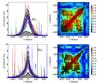 |
Fig. 1 Hα and Hβ line profile variability (left) and autocorrelation matrix (right). The pixel-by-pixel median of the line is shown as a thick blue line. The pixel-by-pixel rms is shown as the thick black line and shaded area. The zero velocities/wavelengths of the lines are marked as dashed vertical lines. The correlation coefficient (estimated as a Spearman rank correlation with value r and false alarm probability p) is shown on the right in the colour scheme, with the black contours marking the high significance (p> 10-5) areas with r = 0.6,0.7,0.8,0.9. |
The emission lines are very complex. To find a proxy to measure line variability and dynamics, we take a two-step approach:
-
First, we explore the pixel-by-pixel variation of the BC withoutassuming any particular model for the line. This method was usedby Lago & Gameiro (1998) and Alencar et al.(2001) to study variability patterns in T Tauri stars. It allows us toidentify the dynamical effects that dominate the changes in theline profiles, which parts of the line have the highest variability,and whether variability affects all parts or velocity components ofthe line similarly. It also allows us to check for correlationsbetween the different velocities and lines.
-
Second, we use a multi-Gaussian fit to reproduce the line emission and explore the variations in intensity, RV, and width of the various Gaussian components. This is particularly useful for studying the behaviour of the NC, whose velocity, amplitude, and width do not depend on the particular choice of Gaussian fit. Since most of the metallic lines have weak (often undetectable) BC with poorly resolved profiles, the metallic line analysis refers almost exclusively to the NC of the lines.
3.1. A pixel-by-pixel dynamical view of the broad component
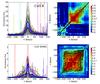 |
Fig. 2 Same as Fig. 1 for the Ca II K (top) and 8498 Å (bottom) lines. The pixel-by-pixel median of the line is shown as a thick blue line. The pixel-by-pixel rms is shown as the thick black line and shaded area. The zero velocities/wavelengths of the lines are marked as dashed vertical lines. The correlation coefficient (estimated as a Spearman rank correlation with value r and false alarm probability p) is shown on the right in the colour scheme, with the black contours marking the high significance (p> 10-5) areas with r = 0.6,0.7,0.8,0.9. |
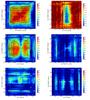 |
Fig. 3 Pixel-by-pixel velocity cross-correlations between different lines. From top to bottom, left to right: Ca II 8498 vs. 8662 Å, Ca II K vs. Ca II 8498 Å, Ca II 8498 Å vs. Hα, Ca II 8222 Å vs. He I 5875 Å, Hα vs. He I 5875 Å, and Ca II 8498 Å vs. Hβ. The correlation coefficient (estimated as a Spearman rank correlation with value r and false alarm probability p) is shown on the right in the colour scheme, with the contours marking the high significance (p> 10-5) areas with r = 0.6,0.7,0.8,0.9. |
To explore the pixel-by-pixel variation of the emission lines, we first resampled all the spectra to the lower FEROS resolution. The richness of features in the EX Lupi spectra is such that finding a proper normalisation at all wavelengths is very hard. Therefore, for each line the spectra are normalised to the local continuum levels, measured on both sides of the line on parts of the spectrum that are not affected by emission or absorption lines. We then estimated the median and standard deviation of the emission line at each pixel after clipping to remove bad pixels and cosmic rays. The procedure was repeated for all the broad lines along the extent of the BC line wings.
We also explore to what extent the emission at a given velocity is correlated with the emission at any other velocity within the same line, and how different lines are correlated with each other. If we attribute each velocity bin to a particular gas parcel (or parcels) moving at the same rate, the autocorrelation matrix and the two-line cross-correlations reveal which parts of the system may be connected. Nevertheless, there could be material moving at the same projected velocity, but coming from different physical locations, which can alter the pixel-by-pixel velocity correlations. In addition, Dupree et al. (2012) demonstrated that there are significant temporal variations of the order of hours between the various accretion indicators (including the Balmer H emission, the veiling continuum, and the He I lines) in a clumpy-accretion episode. Since the reaction time differences between various lines are longer than our exposure times, this could dilute the correlations.
Figures 1 and 2 show the line variance, the median value, and the autocorrelation matrix at different velocities for the hydrogen and Ca II lines. The hydrogen Balmer lines are, as expected (Edwards et al. 1987; Appenzeller et al. 1989; Muzerolle et al. 2001), very complex and asymmetric. They often have self-absorptions that may correspond to colder wind/infall components, which can dilute the correlations or otherwise produce very complex patterns. The Hα line is particularly remarkable because it has a profile with both blueshifted and redshifted absorptions. The blue part of the spectrum shows a higher variability, probably due to the presence of a variable wind. Part of the redshifted emission may also be suppressed by self-absorption in an optically thick accretion flow. The maximum velocities observed in the red and in the blue increase when the strength of the line increases, as observed during outburst and expected in the case of fluctuations of the accretion rate (Natta et al. 2004). If attributed to free-fall (infall-dominated) alone, the maximum velocities (±300 km s-1) would suggest material flowing onto the star from distances of ~2 stellar radii, considering M∗ = 0.6 M⊙ and R∗ = 1.6 R⊙. There is also a tendency of the line to become more symmetric when its intensity (and thus accretion rate) decreases, also a sign of the complex profile being strongly affected by self-absorption. The higher Balmer lines become increasingly symmetric, with similar variability on their blue- and redshifted sides. For the Hα and Hβ lines, we find a strong correlation between the blue- and red-shifted parts, while the correlation of the line wings with the central part of the line is significantly lower. This is a further sign that the zero-velocity components may be saturated and/or produced in several spatially different or very extended locations.
The Ca II lines, especially the IR triplet (only covered by FEROS) also show very broad components. The Ca II IR triplet BCs have a remarkable profile reminiscent of the outburst profiles of the metallic lines (SA12): the BC of the line changes from blue- to redshifted within timescales of days, spanning a wide range of velocities. The BC also decreases to be nearly undetectable when the accretion rate decreases (see Appendix C). Both the median line profile and the pixel-by-pixel standard deviation are very symmetric, in strong contrast to the individual lines, showing that the variability in the blue and in the red is very similar, but independent. The Ca II 8542 Å line falls partially in the FEROS spectrograph gap, but it appears similar to the other two Ca II IR triplet lines. The Ca II IR triplet is thus consistent with bulk motions of parcels of gas that are sometimes blueshifted and sometimes redshifted, rather than to related processes (such as infall/accretion and accretion-powered wind) that produce correlated blueshifted and redshifted features. At first order, the lack of anticorrelations is also a problem for the companion scenario, where we would expect the RV shift to increase one side of the line while decreasing the other, although the shift could be significantly smaller than the BC velocity widths and thus hard to detect. Although the Ca II line forms closer to the star, this asymmetric motion is consistent with the CO observations of Goto et al. (2011) and Banzatti et al. (2015) and with the day-to-day variations in the line profiles during the 2008 outburst (SA12), suggesting that the asymmetric, rotating/infalling structure that fills in the inner disk probably continues onto the inner magnetospheric accretion region. The Ca II H and K lines have asymmetric profiles with a blueshifted absorption that is in part correlated with the wings on the redshifted side of the line, although the velocity range is small compared to the H Balmer lines or the Ca II IR triplet1.
We can take a further step in exploring the connections between different lines and velocities by calculating the pixel-by-pixel cross-correlation between different lines (Fig. 3). The cross-correlation matrix for the Ca II 8498 and 8662 Å shows the same pattern as the autocorrelation matrix of each line, a sign that they are nearly identical, as expected. There is an anticorrelation between Ca II K and Ca II IR, likely due to S/N effects and variations of the accretion rate. A higher accretion rate produces strong Ca II IR, but also a higher blue continuum, and thus a lower peak over the continuum of all the UV and blue lines. At low accretion rates, the excess blue continuum decreases, and since EX Lupi is a M0 star with little blue/UV emission, the continuum at short wavelengths is noise-dominated and the strength of blue/UV lines over the continuum is artificially increased. A similar anticorrelation appears between Hα and CaII K: the Hα blue and red wings are anticorrelated with the Ca II K line. Since the red and blue Hα wings (and the near-UV continuum) grow when the accretion rate increases, the Ca II K peak over the continuum decreases if the Ca II K line flux does not increase at the same rate. This is a sign that we need to be careful when comparing lines at different wavelengths.
Cross-correlation reveals that the wings of Hα and the BC of the Ca II IR triplet lines are correlated (Fig. 3), a sign that the strength of the Ca II IR triplet BC depends on the accretion rate, although the velocities and line profiles change in an independent way. There is no significant correlation between the Hα peak and the Ca II IR lines, probably because Hα is strongly saturated. The cross-correlation between the Ca II IR triplet and the He I lines does not give any significant result. This suggests that both lines respond to different physical processes that are likely to happen in different locations and at slightly different times (Dupree et al. 2012).
3.2. Multi-Gaussian fit and radial velocities
The second step involves studying and quantifying the strength, width, and radial velocity of the different emission lines. We fitted small sections of the normalised and continuum-subtracted spectrum (typically, ±100 km s-1 around the line for narrow features, and up to ±300 km s-1 around features with BC) with a multi-Gaussian model. For the strongest, complex lines (Hα, Hβ, etc.), any attempt to use simple multi-Gaussian fitting or interpretation is impossible. The He I and He II lines are less complex, as are the metallic lines (Ca II, Fe I, Fe II, Ti II, Si II, Mg I, among others). These weaker emission lines are the main subject of this section.
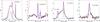 |
Fig. 4 Some of the multi-Gaussian fits for one of the dates (JD 2 455 674.82443). The normalised, continuum-subtracted observed spectra are displayed as thick black lines. Individual Gaussian components are plotted as thin lines (colours: green, red, blue, cyan). The combined fit is plotted as a magenta thick line. The zero velocities of the central line are also marked with a vertical dotted line. The plots are labelled with the line(s) elements and wavelength. Note that the very complex shape of the continuum around the Fe I 5269/70 Å lines is better fitted by two strong Gaussians, one in emission and the other in absorption (partly out of the figure). These BC have no physical meaning/interpretation, but allow us to extract properly the strong NC of both lines. |
Our aim is not to find the best mathematical fit, but a simple and robust one that can be used for all the data taken at different dates in order to compare them. As a result, a direct physical interpretation may be difficult, but we will be able to detect, quantify, and explore differences in velocities, widths, and amplitudes in the spectral lines. A multi-Gaussian fit is strongly degenerated, so we imposed a few restrictions based on the visual aspect of the lines and continuum to make the models comparable. We used three Gaussians with independent amplitudes, widths, and wavelength offsets. In some cases where more than one line is present within the considered section, we added a fourth Gaussian component (for instance, to fit the O I triplet at 7774 Å). The lines have a NC+BC structure, so one of the Gaussians needs to be narrow, with a width of 8−30 km s-1 (or two narrow Gaussians in the case of two nearby narrow lines such as Fe I 5269/70 Å). The Gaussian amplitudes are constrained to positive values, except for the He I lines, which are better fitted by including one Gaussian component in absorption, and cases where the emission line appears on top of a photospheric absorption feature (e.g. Fe I 5269/70 Å). All fits were visually inspected, and any parts of the line or continuum that were affected by spikes were removed. Figure 4 shows some examples of the multi-Gaussian fits for various lines.
We find that the NC fit is independent of the assumptions made on the fitted Gaussians. Nevertheless, fitting the BC is strongly degenerated, as most spectra can be equally well fitted by various very different Gaussian components. Therefore, the results of the BC fitting have to be handled with care, while the amplitudes, velocities, and widths of the NC are very robust. Details on individual lines are given in Appendix E.
3.2.1. Analysis of the narrow component
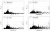 |
Fig. 5 Some examples of GLS periodograms for different lines. The 7.41d period (marked as a blue dashed line) becomes increasingly significant as we move to lines with higher excitation potentials. The FAP are marked as dotted horizontal lines and labelled accordingly. The situation observed for Mg I is typical of the rest of metallic lines labelled as having several peaks. |
Our detailed multi-Gaussian fit allows us to obtain more accurate velocity measurements than the automated fitting and averaging method in K14, allowing us to treat each line independently. Our discussion here is thus focused on the velocity modulation of the strong NC emission lines. Weaker narrow emission lines are noisier, although they are consistent with the same modulation. Kóspál et al. (2014) noted that the NC of the emission lines shows RV patterns that are off-phase with respect to the RV curves of the photospheric absorption lines. To quantify the velocity modulation of the NC emission, we run a generalised Lomb-Scargle periodogram (GLSP; Scargle 1982; Horne & Baliunas 1986; Zechmeister & Kuerster 2009) to search for periodic signals. Each line has a very stable characteristic line width, which can be as narrow as 9 km s-1 for some Ti II lines and as broad as 20 km s-1 for He I lines. The data were clipped based on the NC line width, since significantly broader lines are usually contaminated by the BC, while very narrow ones are often affected by spikes or low S/N, leading in both cases to inaccurate NC velocities. The errors in the line fit can be very complex, considering that the sum of Gaussians is a degenerated fit. Therefore, we estimate that the errors in the velocity are proportional to the line width and inversely proportional to the line strength, including a factor to account for the finite spectral resolution, resulting in typical errors well below 0.5 km s-1. The clipping procedure leaves us from 30 to over 50 points per emission line, with the strongest lines having more valid points than the faint, low S/N ones. The results of the GLSP periods and false-alarm probabilities (FAP) are summarised in Table A.2.
We find that some of the lines show significant periods similar to the RV period of the photospheric absorption lines, 7.41d (K14). In most cases, rather than a single period, we observe a strong modulation and a signature of quasi-periodicity, with several similarly significant peaks in the 7−8d range. Periods of 8.09 and 7.19d are frequent, and could be aliases of the 7.41d period. The strongest signature is observed for the He II 4686 Å line, for which we recover the period obtained for the photospheric absorption lines by K14, although this line is not particularly strong compared to others. Some of the strongest lines, such as the Ca II 8498 and 8662 Å lines, show no significant periodicity (as expected from the lack of modulation; Fig. 6). Therefore, the presence (or lack of) significant periodic signatures is not an issue of S/N2, but is instead due to the underlying structure of the emitting material. Figure 5 shows some examples of the resulting periodograms, and details about every individual line are summarised in Table A.2.
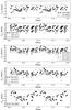 |
Fig. 6 Phase-folded curves (using the photospheric absorption line period and phase, which is nearly identical to the He II 4686 Å line period and phase) for several of the observed NC of lines. We note that two 7.417d periods are plotted for clarity. The dotted line represents the RV curve measured for the photospheric absorption lines (K14). |
Plotting the NC central velocities against the He II (or K14) period reveals that most of the lines are consistent with similar sinusoidal periodic modulations with the same period than the RV signatures of the absorption lines (Fig. 6). The RV modulation depends on the line considered, ranging from lines that show hardly any modulation (such as the NC of the Ca II IR triplet), to others where the amplitude of the RV modulation is much larger than the RV amplitude of the photospheric absorption lines (e.g. He I, He II show modulations up to 8 km s-1 peak-to-peak amplitude, compared to 4.36 km s-1 for the photospheric absorption lines). Among the parameters in the Gaussian fit (RV of the centre of the Gaussian, amplitude, and width), only the RV shows a significant modulation. The line width is remarkably stable within the same species and transition, and the amplitude shows low-significance modulations that could be related to orientation of the emitting structure (Sect. 5). Interestingly, although the BC appear more intense during higher accretion phases, there is no evidence that the variations of the accretion rate for the quiescence data produce any significant change in the properties and velocities of the NC (see Appendix C).
Most of the lines are redshifted by different amounts (from less than ~1 km s-1 for the Ca II IR lines, up to ~5 km s-1 for He lines) with respect to the zero-point stellar velocity (−0.52 km s-1; K14). This suggests that the lines are not produced at the stellar photosphere, but in a slightly infalling structure. Since the redshifted velocities of the lines also vary from element to element, the various species are not produced in the same place of the structure. Significantly redshifted He I lines (compared to the stellar velocity and to Fe I/II lines) have been also observed in other stars by Beristain et al. (1998, 2001) and Gahm et al. (2013).
Figure 6 also reveals a systematic offset between lines from the same multiplet. This is particularly remarkable for the 8498 and 8662 Å lines of the Ca II IR triplet, and can be explained by differences in the optical thickness of the lines. Although the third component of the triplet, at 8542 Å is very close to the FEROS spectrograph gap, the NC is often within the FEROS coverage, displaying a behaviour comparable to the 8498 Å line in peak intensity and zero-point velocity, while the 8662 Å line is redshifted by ~1 km s-1 with respect to them and has a lower peak intensity. The 8498 Å NC line has a tendency to being narrower than the other two. Hamann & Persson (1992) noticed the difference in intensity and thickness of the 8498 Å vs. 8542−8662 Å lines in CTTS (assuming a chromospheric origin for the lines) and offer two explanations: The 8662 Å reduced intensity could be caused by its upper level being partly depopulated by interactions between the Ca II H line (which shares the same level) and the Hϵ line. Regarding the line thickness (and, in our case, also probably the offset velocity variation), an explanation may lie in the 9-times lower opacity of the 8498 Å line, compared to 8662 Å. This can cause a change in the line profile (the optically thicker line is broader) and also means that the 8498 Å line would be produced in a deeper place, compared to the 8662 Å line. Hamann & Persson (1992) suggest a temperature inversion causing a source function inversion in the zone where the Ca II IR triplet originates, which would mean that the 8498 Å line would be produced in the deepest place, the 8662 Å line would be produced at the minimum, and the 8542 Å line would originate where the temperature raises again. Such a situation could also arise in a post-shock cooling region (Sect. 4.1). A similar explanation could also fit the differences between the Mg I 5167/5172/5183 Å triplet, which also shows differences in strength and RV between the 5167 Å line and the rest, although the 5167 Å line coud be in part affected by a strong, nearby Fe I line.
3.2.2. Analysis of the broad component
We also searched for periodic signatures in the strong, rapidly variable BC of the Ca II 8498 and 8662 Å lines. The span of peak velocities is over ±100 km s-1, and similarly good fits may show variations by several tens of km s-1. We first compared the independent fits for the 8498 and 8662 Å lines to check how reliable and stable the BC velocity determinations are. We estimated the Spearman rank correlation for all the three Gaussian fits components: amplitude, central wavelength, and width. Cross-correlating the results for the two lines (see Appendix D for details) shows that there is a very strong correlation between the individual parameters of both lines. This means that we are obtaining similar fits for these two very similar lines, despite variations in the noise and continuum between both. For most of our data points, a single broad Gaussian dominates the BC fit, and the second broad Gaussian component is often marginal and/or poorly constrained, which leads to degeneracy.
For a given line, we checked the cross-correlation between the fit parameters, to investigate how changes in one of the components (NC or the two broad Gaussian components) are reflected in the other ones. Appendix D details the procedure and results. We find that the NC is relatively independent in amplitude and central velocity from the BC. Only the width of the NC seems to increase slightly when the intensity of the BC increases. This could be a sign of an increase of the local turbulence at near-zero velocities for higher accretion rates (expected by comparison with the outburst observations; SA12), but it could also reflect contamination of the NC by a more intense BC. The centre and the amplitude of the two BC Gaussians are correlated, so their velocity increases when the amplitude of the BC increases. This is similar to what we observed during outburst: at higher accretion rates, the material seems to be dragged from more distant places or, conversely, more distant parts reach the required temperature and density to produce emission lines (SA12). This is consistent with accretion models for the Hα line (Lima et al. 2010). We do not find any significant correlation between the blueshifted and redshifted BC Gaussian components, which is a sign that they are independent and not caused by the same physical process (for instance, an increase in the accretion rate triggering an accretion-powered wind). They seem only linked by temporal variability, as expected for bulk motion of material rotating as it falls onto the star.
Finally, we searched for periodic signals in the BC. The centring errors for a broad Gaussian are much larger than for the NC, so we also checked the location of the peak of the BC emission (after subtracting the NC), which is less affected by the choice of fit. We only consider those data points where the amplitude of the BC is ≥0.3 (over the normalised and subtracted continuum, well above the noise level). The results of the GLSP for the BC are listed in Table A.2. For the BC Gaussian components, the periodicity analysis is not conclusive, mostly due to the small number of data points. The BC peak shows multiple low-significance periods, in agreement with the periodic or quasi-periodic signatures in the 7−8d range observed in the NC of the lines. Examining the shape of the BC line (see Appendix E), we also find a trend with the phase of the NC/photospheric absorption lines, especially for the cases with strongly bluesifted BC. This suggest that there is a common mechanism causing the velocity modulations of all emission lines and that the NC and BC are physically related.
4. Dynamical and physical models for the spot, the star, and the accretion column
In this section, we construct simple models to explain the RV signatures of the emission lines in EX Lupi, and explore the possibilities of a stratified 3D hot structure to reproduce the dynamics and the strengths of emission lines. We assume that the footprint of the accretion structure behaves like a hot spot. A hot spot on the stellar surface would cause a clear modulation of the photospheric absorption lines as shown in Fig. 7, and could mimick the RV signature caused by a companion. The main challenge for the spot scenario is that different lines have different RV modulations, which is inconsistent with plain flat hot spot models. Nevertheless, accretion can alter the vertical temperature structure of the photosphere, suppressing normal absorption line formation in the accreting region. The extent to which the absorption is suppressed will depend on the strength and depth of the formation of the lines concerned (one example being the Li I 6708 Å line, the only photospheric line that still presents a small absorption component during outburst; SA12). The diversity of the amplitudes and the zero-point offsets between lines is a sign of a more complex 3D accretion structure, extended in the vertical (radial) direction and having a temperature and density gradient within the flow and/or across the accretion column. This is consistent with the observations during outburst (SA12), and with evidence found in other T Tauri stars (Dupree et al. 2012; Petrov et al. 2014).
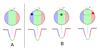 |
Fig. 7 Scheme of the effect of a hot spot that rotates with the star affects the photospheric absorption lines. In A) we show the different parts of the stellar photosphere that produce the photospheric absorption lines. B) shows how the line is affected when a hot spot is included. When the absorption deficit associated with the spot appears blueshifted, the centre of the photospheric lines seems to move towards the red. When the spot appears redshifted, the centre of the absorption line appears shifted towards the blue. Small emission lines are visible within some of the photospheric absorption lines, tracking the local rotational velocity of the part of the stellar surface where the line originates. Non-photospheric lines or lines that are particularly strong on the spot could appear simply as emission lines over the continuum, without any underlying absorption. |
4.1. Dynamics of narrow and broad components and their RV signatures
Amplitudes and offsets of a sinusoidal fit to the emission line signatures.
The location of the line-emitting region can be inferred by modelling the observed dynamical signatures and RVs (Fig. 6). If the NC lines are produced in a localised accretion spot structure, stellar rotation would affect their RVs imprinting a sinusoidal modulation. A similar scenario has been proposed for UV lines, for which some stars are also consistent with accretion-related spots getting in and out of view as the star rotates, and showing different lines-of-sight depending on whether they form in the accretion column or at the associated spot (Romanova et al. 2004; Ardila et al. 2013). Simulations predict that the coverage of the spot decreases as the density of the accretion column increases and at small misaligment angles between the stellar rotation and the magnetic moment (Romanova et al. 2004). Given that the accretion structures in EX Lupi are expected to be very dense to produce the observed emission lines (see Sect. 4.2), accretion models would favour very localised spot(s). The NC emission lines present a sinusoidal modulation with the same periodicity as observed for the absorption lines (Fig. 6), but variable amplitude and zero-point shift (Table 1). For lines with lower excitation potentials, the significance of the periods is lower and the signature is quasi-periodic rather than purely periodic. This can happen if they are produced in more extended and potentially messy structures (Fig. 8).
The amplitude is fairly constant within a given species (e.g. He I, Fe I, Fe II), although there are significant shifts in the zero-point velocity, which is always redshifted. The maximum shift is observed for the He I lines, which is similar to the results of Beristain et al. (2001) on a large sample of CTTS, although the fact that this line could be in part affected by a redshifted absorption (due to wind, for instance; Sect. 3.2) could also led to a higher redshift. Differences in zero-point velocity can also result from differences in the optical thickness (and thus depth) of the lines (Sect. 3.2.1). The differences in profile/velocity between high- and low-temperature lines would be associated with different parts of the accretion structure. Detailed models (Romanova et al. 2004, 2011; Ardila et al. 2013) have suggested various possibilities, ranging from vertical stratification (e.g. in an accretion structure with an aspect ratio where photons can easily escape through the walls), to horizontal stratification across the accretion structure (where the low-density, cooler material at the edges of the accretion column would also show a slower-than-free-fall motion). A further possibility, the presence of several accretion columns with various densities around the stellar surface, appears unlikely for EX Lupi, given that all lines show a very similar modulation (period and phase). An exception could be the Ca II IR NC lines, which do not show modulation and could be produced in a more uniform way over the stellar surface.
We can use the observed sinusoidal modulation to investigate the typical location of the emitting structure (Romanova et al. 2004). The post-shock region at the bottom of the accretion column would be similar to a plage as seen in active stars (Ardila et al. 2013; Dumusque et al. 2014), although in this case, our plage would be 3D and stratified in density, velocity, and temperature. If a plage (or accretion structure) is at a low latitude, it would only be visible during about half of the rotational period, producing an incomplete sinusoidal modulation (from blueshifted to redshifted; the part from redshifted to blueshifted would not be visible). We observe a full modulation, which requires the plage-like structure to be visible during the whole rotational period. If we observe the star under an inclination angle i, this happens for latitudes higher than i (or, in spherical coordinates, θ< 90−i). The observed modulation would be caused by rotation and the 7.41d period would correspond to the rotational period of the star.
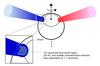 |
Fig. 8 Cartoon of a star with an accretion column that is visible at all times due to the stellar inclination and whose emission lines suffer Doppler shift as the star rotates (the observer is located perpendicular to the plane of the paper). The blue (red) column shows the position at which the lines originated in it would appear blueshifted (redshifted) to an observer looking from out of the page. The hashed areas mark the shock region. We suggest that the observed narrow emission lines are produced in the post-shock area, which is stratified in density and temperature. Lines produced in the shock region (He II, requiring very hot and dense conditions) originate in a nearly flat structure, so their periodic signatures are much stronger and less messy than other lines produced in the extended, infalling post-shock region. The BC is produced in the accretion column before the pre-shock region, showing higher velocity offsets as they rotate with/around the star. Not to scale: we note that the shock region is at a very small distance over the photosphere, compared to the stellar radius. |
For an emission line produced in a small spot located on the surface of the star at spherical coordinate θs, the rotation of the star will change the central velocity of the line following  (1)Here,
  is any zero-point velocity that the system or the emitting zone may have (including the stellar velocity, V0, and any systemic velocity in the accreting structure, such as a systematic redshift in an infalling component, Vz in Table 1), P is the rotational period of the star, φ corresponds to the phase angle (from 0 to 2π), and vsini is the projected rotational velocity of the star. If the spot does not change its latitude during the time we observe it, we obtain a sinusoidal modulation with a RV amplitude that depends on the viewing angle i and the spot location θs. A purely polar spot (θs = 0; such as the one proposed by Dupree et al. 2012 for TW Hya) suffers no modulation. For an equatorial spot, the RV amplitude is largest, although it will not be visible at all times. The maximum RV that can be observed in the emission lines produced at the surface of the star is thus vsini. Lines originating at some distance (d) over the surface of the star could have RV amplitudes up to 2π(R∗ + d) sini/P, assuming that the line-emitting structure rotates as a solid with the star3. Similarly, if the extended structure where the lines are produced is displaced off the radial direction (for instance, trailing the star or extended along the stellar surface), we would expect to observe some phase shift between lines originating at various altitudes. Although significant differences in zero-point velocity and phase are found comparing various lines (Table 1), optical depth differences between lines and unresolved absorption (e.g. wind components) could also produce changes in both measured quantities that cannot be properly estimated without detailed radiative transfer models.
Assuming that the period is 7.417d and vsini = 4.4 km s-1, the system inclination angle i would be 23.8−25.5 degrees (for radius 1.5−1.6 R⊙). For the He II line, we observe a mean amplitude of about 3 km s-1, corresponding to θs ~ 43 degrees (latitude ~47 degrees). For an inclination of 23.8−25.5 degrees, this is compatible with a spot that is visible at all times, in agreement with the observed modulation.
The information in Table 1 can be used to infer the relative location of the various species along the emitting region, although for species with a wide range in excitation conditions and critical densities (e.g. Fe I and Fe II), line strength and opacity differences make this stratification difficult to identify. We explore two options for stratification: along the extended spot vs. across the spot (Ardila et al. 2013). In the first case, material closer to the shock region would be expected to be hotter and denser compared to material closer to the stellar photosphere, and the relative velocities would depend on a mixture of infall and magnetic/gas pressure. In the second, the edges of the post-shock structure would be cooler and less dense, and simulations predict it to show slower infall velocities compared to the hot and dense column centre (Romanova et al. 2004). This situation is analogous to the observations of UV lines in CTTS (Ardila et al. 2013).
The He II line has by far the strongest requirements regarding high temperature and density, which would require formation relatively close to the shock and/or deep within the post-shock structure. In both cases, this spatial restriction would favour a stronger rotational modulation, compared to other lines, which is also observed. Depending on the velocity structure in the shock/post-shock region, its null zero-point velocity shift could suggest excitation very close to the shock and with a strong magnetic/gas pressure support accounting for the lowest infall velocity. In the case of stratification across the column, He II would be expected to form in the innermost part, although in this case its expected infall velocity would be higher than for lines formed in the periphery (Romanova et al. 2004). The difference in phase could be caused by a higher location on the post-shock structure (compared to the stellar photosphere) or by a bow-shaped spot where the density varies along the stellar longitude (Romanova et al. 2004).
The He I and metallic lines would be produced in cooler, less dense parts of the post-shock region. Their small redshifted velocities suggest that the material, although basically at rest (owing to magnetic/gas pressure), is still accreting or infalling. Taking into account the phase differences, after He II, most of the Fe II emission would be produced closer to the shock area or to the denser part on a bow-shaped spot (having the next largest phase difference and lowest infall velocity). He I lines also require hot and dense material. The nearly zero phase difference observed for He I lines and the relatively large infall velocities (if blueshifted absorption due to wind is negligible) would in fact suggest an origin very close to the stellar surface, although the higher He I abundance (compared to metals) can also result in emission over larger areas/volumes, including more extended parts over the stellar surface and perhaps winds. Fe I and Mg I lines would be mainly emitted in an area with lower temperature conditions, comparable to the photospheric temperature or conditions of G or F stars. For an infall velocity of 4.5 km s-1 (typical of the He I lines), the material should be falling from 1.4 × 10⁻⁴R∗ (~160 km) over the stellar surface. Although gas/magnetic pressure and turbulence counteract the infall, models suggest that fully ionised post-shock columns have sizes of the order of 102−105 km (Dupree et al. 2012; Ardila et al. 2013), compatible with our findings of a relatively compact region compared to the stellar radius. Figure 8 shows a scheme of the proposed configuration.
We can also use Eq. (1) to investigate the effects of such emission lines on the RV of the absorption lines. We can model a photospheric absorption line using a Voigt profile that reproduces a typical, unblended photospheric absorption line. We then add a small emission component with a central velocity that has a sinusoidal modulation such as that shown in Eq. (1). A continuum veiling contribution can also be added. We estimate the apparent RV variation of the resulting absorption line by cross-correlation. The modification of the stellar photosphere by the proximity of an accretion hot spot can be very complex, depending on plasma parameters, and can also contribute to powering a stellar wind (Orlando et al. 2010, 2013). Therefore, this analysis does not pretend to derive strong constraints on the properties of the line-dependent veiling, since it involves too many free (or poorly constrained) parameters, but to demonstrate that a simple accretion-plus-rotation model can explain simultaneously the observed RV signatures in the emission and the absorption lines.
We first considered the effect of the narrow emission lines, finding that although the presence of a small NC within the line can produce RV offsets as large as the observed RV amplitudes, they also produce a very strong distortion of the line profile, which is not observed (some lines have narrow emission-line cores, but they were excluded from the RV analysis in K14). We then consider the effect of a BC in emission on the absorption line. Although BCs with emission over the continuum are only seen in certain lines (e.g. Ca II IR triplet, strong Fe II lines such as the 5018 Å and 4923 Å lines), we also see clear evidence of line-dependent veiling in EX Lupi, as proposed by Dodin & Lamzin (2012) for other CTTS. A single veiling factor (or a slowly changing one, such as can result from a black-body approximation to the veiling) cannot reproduce all the lines, even if we restrict ourselves to a very small portion of the spectrum (see more details in Sect. 4.2). This is a sign that many of the absorption lines, if not all, have a line-dependent veiling or extra emission that fills part of the absorption line and that is at least as broad as the absorption line itself (to avoid distorting the line profile). As the accretion rate increases, the line-dependent veiling would increase, filling in the whole absorption line and eventually showing as a broad emission profile for very high accretion rates, as observed in outburst (SA12).
Figure 9 shows that, for reasonable values of the BC width and amplitude, it is possible to reproduce the observed RVs while avoiding a significant distortion of the line profiles and symmetry. Our simple model assumes that the rotationally modulated BC in emission has a Voigt profile (with various Gaussian and Lorentzian contributions, γ). A Gaussian core about 3−4 times broader than a typical photospheric absorption line avoids introducing large distortions in the line profile. We also consider a BC strength that results in veiling factors for the line between 0.25−0.65, and that it has a peak-to-peak velocity amplitude in the range of 10−30 km s-1 and a few km s-1 net redshift (as observed; Table 1). A velocity amplitude of ~20 km s-1 would correspond to a distance of about ~5.7 stellar radii (assuming solid-body rotation and θs ~ 43 degrees), compatible with material near the edge of the stellar magnetosphere. We also include a “classical” continuum veiling as a constant emission factor that dilutes both the photospheric absorption line and the wings of the emission line. Blending of nearby lines (which often occurs in the blue part of the spectrum) could also result in a relatively flat extra emission over the real continuum. The broad line causes a rotationally modulated tilting continuum that changes the apparent RV of the line. With the strongest change being in the broad line wings that always fall out of the absorption line, the line bisector distortion is minimal and comparable to the distortion observed in K14. Checking the two bisector parameters explored by K14 (the bisector velocity BVS and bisector curvature BC, see K14 for details), the variations observed in our model are comparable to the observations of the photospheric absorption lines.
This simple model can reproduce a RV modulation very similar to the one observed. A small net redshift and/or a non-Gaussian profile (adding Lorentzian wings) can produce the observed red-blue asymmetry in the RV curve (interpreted as eccentricity in the companion scenario). Further asymmetries in the observed curve could be caused by the emitting region not being entirely symmetric4 (owing to occultation effects, or to variations in the observed projected velocity for an extended spot as the star rotates), or by having a small phase offset (which would happen if the accretion structure is trailing the star or if the spot is extended along the stellar surface). As long as the period of the line-dependent veiling is maintained, small variations in the strength of the lines would not destroy the global modulation.
We thus conclude that the most complete explanation of the observed RV modulation of the photospheric absorption and the emission lines is offered by assuming a modulation induced by line-dependent veiling throughout the absorption-line spectrum. It also shows that the phenomenon of line-dependent veiling by broad lines may be one of the worst-case scenarios for detecting the presence of companions in accreting stars, given how robust the signal is to small variations in the accretion rate, and how weak the induced line asymmetries can be if the BC is significantly broader than the photospheric absorption lines, being diluted with emission from nearby lines and/or extra classical continuum veiling. If most photospheric lines are affected by line veiling, distinguishing this effect from any other periodic modulation (such as the one induced by a companion) may be very hard.
This model requires that the accretion-related structure is stable over several years. The signature does not seem affected by the strong 2008 outburst (although there are only 3 points taken before the outburst), suggesting that the accretion structures infalling onto this star are extraordinarily well-fixed to the stellar structure/magnetic field. Even though the accretion rate varies in time and is probably very clumpy, it would be a case of remarkably stable accretion columns with very little instability (Kurosawa & Romanova 2013). Checking the long-term stability of the signal will be also a strong test for the proposed accretion column scenario.
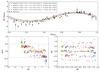 |
Fig. 9 Results of our toy model for the RV signatures (upper panel), and bisector velocity shift (BVS) and curvature (BC; lower panels). It shows the kind of RV modulations that can be induced on a photospheric absorption line by an emission component (broader than the absorption line) that shows a rotational modulation. “P” denotes the peak value of an emission component with a Voigt profile with Gaussian width σ and Lorentzian contribution γ. “Cont” marks the classical veiling continuum added to the model. “A” denotes the RV amplitude of the emission line (maximum RV offset for a sinusoidal modulation), and “RS” is the zero-point redshift of the line. The dashed box shows the values of the bisector velocity as measured by K14, which are similar to those derived from the toy model. Although there is a slight BVS slope, the typical errors at this level can make it very hard to distinguish. |
4.2. Physical conditions in the accretion column
We also explore whether the observed mean spectrum (obtained by combining all the normalised observed spectra) can be reproduced as the sum of a stellar template, a classical veiling continuum (constant over small wavelength ranges) and emission lines originating in a region with a given temperature (T) and electron density (ne). Dynamics and BC emission are not considered in this simple model. We do not attempt to model the H Balmer series, Na I D, Ca II IR triplet, or other broad lines (or BC) since they are very complex and self-absorbed. We also do not have high enough S/N to constrain line ratios and physical conditions for the BC (which was, however, possible during outburst; SA12). Lines with different excitation potentials and critical densities allow us to explore the structure of the line-emitting accretion column in quiescence (S12; Petrov et al. 2014).
For the photospheric model we consider an effective temperature Teff = 3750 K, log g = 4.0, and vsini = 4.4 km s-1 (Sipos et al. 2009), using the standard template from Coelho et al. (1995). The veiling is considered as a continuum with a certain value over a small wavelength range. The atmospheric model with the veiling continuum should reproduce the observed absorption spectrum, but we find that a simple continuum veiling with a slow dependency on the wavelength cannot reproduce simultaneously all the photospheric lines, even if we only consider a small wavelength range (Fig. 10). This suggests a line-dependent emission component filling in part many (if not all) the emission lines with different strengths.
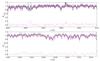 |
Fig. 10 Attempt to reproduce the median EX Lupi spectrum (black line, with standard deviation per pixel marked in grey) by using a rotationally broadened standard veiled by a continuum emission (magenta). The difference between the observed and veiled spectra is shown in pink. A constant veiling cannot reproduce the depths of all lines, even if we only consider a very small wavelength range. The differences are too large to be explained by the standard deviation or time variation observed between the different spectra. |
For the emission line spectrum, we consider only the metallic and narrow lines, including He I and He II, which are dominated by NCs. We first estimate whether the line emission is optically thin or thick, and obtain approximate values (or ranges) for the temperature and electron density in the emitting region. In broad lines, the high velocity gradients ensure that the lines are optically thin (Beristain et al. 1998; Petrov et al. 2014). For EX Lupi, the NC line ratios are nevertheless consistent with partially optically thick emission. We use the atomic data from the National Institute of Standards and Technology database (NIST; Kelleher et al. 1999; Ralchenko et al. 20105) to estimate line ratios in the optically thin approximation, which are proportional to the atomic gf factors for permitted lines (Martin & Wiese 1999). For a transition with upper level k and lower level i, the line strength gifik can be estimated as 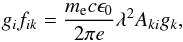 (2)where gi and gk are the level multiplicities (2J + 1), Aki is the transition probability, c is the speed of light, me and e are the mass and charge of the electron, and ϵ0 is the dielectric constant. Comparing line pairs with similar upper-level energy (Table 2, see Table A.3 for a complete list of unblended lines) shows that although some of the lines (e.g. He I) are optically thick and saturated, the metallic neutral and ionised lines (Mg I, Fe I, Cr I, Mn I, Fe II, Cr II) span a broad range where the stronger lines tend to be optically thick and the weaker ones are sometimes optically thin. We also observe significant differences compared with the case of DR Tau in Beristain et al. (1998), such as the suppression of the lines with lower transition probabilities (Aij) and lower excitation temperatures, which point to higher temperatures and densities and/or stronger high-energy irradiation for EX Lupi than for DR Tau, despite its lower accretion rate.
The density can be estimated from the accretion rate (SA12): 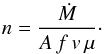 (3)Here, n is the number density, Ṁ is the accretion rate, A is the area of the stellar surface of which a fraction f is covered by the accretion-related hot spot, v is the velocity of the accreted material as it arrives to the shock region, and μ is the mean particle mass. If we consider the observed values for the accretion rate (Ṁ ~ 10-10−10-9M⊙/yr) and the velocity at which the material arrives to the shock region (v = 100−200 km s-1), we arrive at n = 6−120/f × 109 cm-3. We assume that the spot covers a small part (~1%) of the stellar surface (suggested by Grosso et al. 2010 based on X-ray observations, and expected in the case of higher density; Romanova et al. 2004). At relevant temperatures all the metals would be ionised and the H and He would be mostly neutral, producing electron densities of ne ~ 108−1010 cm-3. If the material arrives at the shock region at high velocities (v = 100−200 km s-1), but is deccelerated onto the star at few km s-1 (Table 1) in the post-shock region where NC originate, we can expect the density to increase by up to two orders of magnitude, arriving at ne ~ 1010−1012. These higher values are more in agreement with what we would expect from the nearly equal ratios observed for the Ca II IR triplet, among others. Extra ionisation due to energetic radiation in the accretion shock or in the stellar chromosphere could also increase the electron density in the post-shock area. The presence of extra sources of ionisation were evident during the outburst (SA12), and some extra contribution of ionising UV emission (accretion-related) and by the shock itself (Orlando et al. 2010) is also likely to happen in quiescence.
We also follow Hamann & Persson (1992) to evaluate the electron density based on the requirements to achieve optically thick emission lines in the spectrum (similar for chromospheric emission and an accretion column or post-shock region scenario). The condition for equal flux in a multiplet of emission lines (such as the Ca II IR triplet, or the Mg I triplet) is satisfied when collisional decay dominates over the transition rate, neCki ≫ Aki/τ. This mean τne ≳ 1013 cm-3 for Ca II 8542/8662 Å. Grinin & Mitskevich (1988) suggest that values of τ> 1 for the 8498 Å line, τ> 10 for the 8542 Å line are enough for this. Considering the lower τ values, Shine & Linsky (1974) estimate the minimum threshold density for detection of Ca II emission to be NCaII ~ 2.5 × 10¹⁵ (V/50 km s-1) cm-2. Assuming a solar composition and that most of the Ca is ionised, this results in N(HI + HII) ~2.5 × 10²¹ (V/50 km s-1) cm-2.
In EX Lupi, the BC of the Ca II IR triplet becomes undetectable when the accretion rate is at its minimum (Ṁ ~ × 10-10M⊙/yr). This suggests that the Ca II BC is very close to its optically thin limit, so that ne ~ 1012−1013 cm-3 in the region where the BC originates. If we assume that the accretion rate is constant for the amount of matter that flows through the BC-region into the NC-region, Ṁ = nBCAfBCvBC = nNCAfNCvNC, the relation between the density depends on the velocity ratios of the material, and the areas covered by the BC and NC zones. If there are no different sources of extra ionisation between the two regions, the relation can be transformed into a relation for the electron density:  (4)The velocity widths are about 12−14 km s-1 for the NC and 50−100 km s-1 for the BC, which means by itself an increase in density by a factor of 3.5−8.5. If in addition the accreting structure gets thinner/compressed as it moves into the shock/post-shock region, a further increase in the density is to be expected. This means that in the NC emitting region, ne ≳ 5 × 10¹²−1013 cm-3. We will use this estimate as a starting point in the subsequent calculations. Such density estimates are in agreement with (or slightly higher than) the values derived by Petrov et al. (2014).
Following SA12, we apply Saha’s law for various temperature and electron density values, in order to constrain the temperature and density structure in the accretion columns (Mihalas 1978). Saha’s law works under the assumption that the system is in local thermodynamic equilibrium (LTE). The LTE assumption is questionable, although acceptable in an approximate toy model. We use the NIST line emission calculator to estimate line intensities and ratios for a given T and ne. As in outburst, a single temperature-density pair is unable to reproduce all the lines at the same time. The lack of significant emission from Ti I lines puts a very strong constraint on the typical temperatures in the accretion column. For the relevant densities, a minimum temperature of ~7000 K is needed to make the Ti I lines undetectable compared to Ti II. Regarding the He I/II emission, a temperature between 8000−10 000 K can explain the strength of the 5875 Å and 6678 Å lines, but the formation of more energetic lines (such as the He I 4920 Å and especially the He II 4686 Å lines) require temperatures of the order of 20 000−23 000 K, which would render other elements such as Fe, Cr, and Mg fully ionised.
For our final toy emission line model we thus consider a constant electron density ne = 1013 cm-3 and three different temperatures: 8000, 10 000, and 23 000 K (0.69, 0.86, and 2.0 eV, respectively). We note that in the real situation, both the electron density and the temperature are expected to vary within the accretion column. Since most of the lines are optically thick, the line intensity is simply scaled to match the observations. The final spectrum is obtained by summing the photospheric component, a continuum veiling, and the lines. Figure 11 shows the results of our simple model in several wavelength ranges. Despite its simplicity, our toy model confirms that a temperature stratification is needed to fit the observed emission. A range of temperatures and electron densities is also consistent with our naive picture in Fig. 8, with the most energetic He I and He II lines being dominated by the high temperature component, closer to the shock region, and the Fe II and lower-excitation He I lines being dominated by higher temperature emission than the Mg I or Fe I lines. Further exploration would require a proper line radiative transfer model with detailed physical conditions along the accretion structure, which is beyond the scope of this paper.
Line ratios in the optically thin limit.
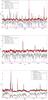 |
Fig. 11 Toy model for the narrow emission lines, obtained by considering an electron density 1013 cm-3 and three different temperatures along the accretion column (8000, 10 000, 23 000 K). The rotationally broadened standard star spectrum is shown in grey, and the individual lines are shown in various colours. The final model, including a constant veiling, is obtained by summing all three components. |
5. Discussion: the star, the spot, and the accretion column
5.1. Critical revision of the origin of the line and RV modulations
The velocity modulations observed in EX Lupi emission lines were first described in SA12, concentrating on the most conspicuous modulations (tens of km s-1) observed during the 2008 outburst. For the RV variations in the photospheric absorption lines, K14 proposed two possible origins: RV signatures induced by a BD companion (with msini = 14.7 Mjup and semimajor axis 0.063 AU) vs. rotational modulation induced by possibly two hot spots on the stellar surface. Both the BD companion model and the classical hot spot(s) model were not able to produce a complete explanation of the observations. Here we propose a 3D accretion column as the origin of the RV modulation of both emission and absorption lines. An accretion hot spot or accretion column is necessary in order to produce the temperature inversion that gives rise to the emission lines. Therefore, if accretion alone is able to explain all the observations, it would offer the most simple explanation without needing to add further elements.
The main caveat of the companion model is that a companion-only scenario cannot explain why the emission and absorption line velocities are off-phase. A tentative solution could be sought if the accretion mostly landed on the BD companion or in a structure connecting both objects (e.g. Artymowicz & Lubow 1996). In that case, we would detect the photoshere of the bright primary (a M0 star, the BD photosphere would not be detected owing to contrast) and the hot spot on the secondary or on the connecting structure. This would produce an anticorrelation between the RV of absorption and emission lines, similar to what has been observed in X-ray studies from accretion shocks in interacting binaries (Donatti et al. 2011; Argiroffi et al. 2012). Since the masses of EX Lupi and the proposed companion are very different, the amplitudes of the RV signatures for both would be very different. Nevertheless, this scenario is inconsistent with the observations. Considering the line with the strongest RV signature (He II 4686 Å line), there is only a very mild anticorrelation: a Spearman rank test gives a correlation coefficient r = −0.20 and false-alarm probability p = 0.20, which is not significant. Figure 6 reveals that the emission line modulation is not simply the scaled stellar RV with a changed sign (which would be strongly asymmetric), but a redshifted symmetric sinusoidal modulation (Sect. 4.1). The timing of the RV cycle as observed in the absorption and emission lines is also in contradiction with the expected signatures in the case of accretion in a binary system (Artymowicz & Lubow 1996) since it would need a variable difference in phase of approximately one-fourth of a cycle, while accretion is most likely to occur along the line connecting both objects. The phase variation between the companion and the accretion would also require the accreted material to move at unphysical variable speeds, which change the relative position between the spot and the companion during the phase. A scenario with spots on both objects would similarly fail, as it would either dilute the signature of the RV of the emission lines or modulate the line thickness (by summing a redshifted and a blueshifted component that change along the orbital phases). It also fails to explain why the RV amplitudes are often larger for the emission lines than for the photospheric absorption lines, and why the shapes of both curves are so different (asymmetric for absorption lines, symmetric for emission lines).
The main caveat of the hot spot scenario in K14 is that it would require the 7.41d period to be the rotational period of the star, which would be hard to reconcile with the vsini and the constraints on inclination from disk models and CO observations. We nevertheless find that vsini = 4.4 ± 2.0 km s-1 (Sipos et al. 2009) reproduces better the observations than the upper limit value of 2−3 km s-1 given in K14. With this higher rotational value, a rotational period of 7.41d would require an inclination angle of 23−25 degrees (consistent with the disk models of Sipos et al. 2009). A low viewing angle was also predicted by Grosso et al. (2010) based on X-ray absorption. The observed velocity amplitude of the NC is also in agreement with an origin in a high-latitude structure, in a star that is seen at a relatively low angle (Sect. 4.1). Moreover, all the NC velocities are redshifted, also in agreement with a relatively low viewing angle where the line-emitting region is always seen infalling (never blueshifted) as the star rotates.
The problem with the hot spot hypothesis in K14 is that models for a classical, continuum-emitting, flat hot spot would require a coverage as large as (or larger than) the stellar surface to produce the RV signatures observed. Such a spot would also produce a luminosity modulation that is not observed in the photometry records. Kóspál et al. (2014) assumed that the spot would suffer occultations as the star rotates, which would increase the luminosity contrast, but a high-latitude spot visible at all times would not induce dramatic variations in the luminosity. In addition, if most or a large fraction of the energy released in the shock structure is emitted in lines (including many metallic UV lines) and not in the optical continuum, photometric rotational modulations may not be evident, while RV modulations would be significantly enhanced with respect to the continuum-only scenario. This situation had been described in other T Tauri stars (usually with strong accretion) and was named “veiling-by-lines” (Dodin & Lamzin 2012, 2013).
The detailed line-by-line dynamical analysis breaks one of the main counter-arguments in K14 against the spot/column explanation, that the RV shifts observed in the emission lines had a smaller amplitude than the RV of the photospheric absorption lines and that the signal periodicity was not significant. This happened because the relative offsets between lines and the various degrees of modulation (for instance, comparing He II with Ca II NC) dilute the global signature when many lines are combined. Once the lines are treated individually (including detailed individual fits), the modulation is strong and significant. This is an extension of what we observed during outburst (SA12), with different lines having various velocity offsets depending on their excitation and physical conditions in the extended non-axisymmetric accretion structures. Petrov et al. (2014) also demonstrated that the stratification in velocities and physical conditions in the accretion columns results in different velocities for lines with various excitation potentials, although in this case the lines were seen in absorption and were not time-resolved.
If the emission lines are formed in a hot spot near or on the stellar surface whose velocity is modulated by the rotation of the star, the largest extent of the spot is visible at zero velocity, so the line would be stronger when the spot is facing us. Despite the substantial variations from day-to-day and epoch-to-epoch in the line strength, there is a low-significance modulation of the amplitude/strength in several Fe II, Fe I, Ti II and Mg I lines. The lines are weaker at zero velocity, and stonger when both the redshifted and blueshifted velocity offsets are largest. Although this is the opposite situation than mentioned above, it is similar to the case of rotationally modulated X-ray emission (e.g. Flaccomio et al. 2005; Argiroffi et al. 2011, 2012). X-ray emission is produced at the bottom of a 3D accretion shock, which results in the accretion column obscuring most of it at zero velocity, while most of the emission should escape through the sides of the accretion column at maximum redshift/blueshift. This effect has been observed for EX Lupi (Grosso et al. 2010). The same explanation could apply to the NC lines, if formed within a vertically extended structure where the emission can escape better along the sides of the accretion structure, instead of from the top. The Ca II IR lines lack these occultation effects and tend to be stronger when the structure is facing the observer, in agreement with their origin in a less embedded, more delocalised structure with lower density and temperature.
The rotational modulation gets increasingly smaller as we go to lines that are produced at lower-density, lower-temperature conditions, such as the Ca II IR line (Fig. 8). Lower-excitation lines require less restrictive conditions for their formation. These can be met over a larger area on the stellar surface (since they are more similar to the conditions at the photosphere of the star), so the RV signature of these NC lines could be diluted and/or appear rather as a quasi-periodic modulation. Differences in the rotation in various parts of the structure are also expected from models, and could lead to quasi-periodic modulations as observed here for the low-excitation lines (Romanova et al. 2004). Deviations from pure solid-body rotation in an extended structure can also dilute the modulation6. The lower temperature, lower density areas will be larger, diluting the signature with a broader range of velocities. Although the periodicity of the BC of the Ca II lines (the only BC detected in most of the spectra) is not significant, it is also consistent with modulations in the 7−8d range. If the material is fed to the star in a non-axisymmetric way, as proposed in outburst (SA12) and confirmed by CO observations (Goto et al. 2011; Banzatti et al. 2015), it could also help to keep accretion confined to a relatively small area on/near the stellar surface, compared to cases where the material approaches the star from all directions. An accretion column/structure that trails the star (or material that is both accreting and rotating) could induce phase shifts in the rotational modulation, which is also observed (Table 1).
5.2. Origin and implications of stable accretion columns in EX Lupi
Accretion in EX Lupi appears to follow a combination of the standard accretion column scenario as an origin for the emission lines in CTTS (Muzerolle et al. 1998, 2001), and the post-shock scenario (Dupree et al. 2012). We find evidence of BCs consistent with an origin before the shock region in an extended accretion column and of NCs produced in a post-shock, slightly infalling structure extending down to the stellar photosphere. The line widths observed in the NC would suggest a less turbulent environment than proposed by Dupree et al. (2012) for TW Hya, being close to the expected thermal broadening for the relevant temperatures. The velocity differences observed between BC and NC are also consistent with the differences between a pre-shock and post-shock region (Ardila et al. 2013). The BC lines require structures with a large velocity span, which could be due to spatially extended rotating/infalling packages of gas, although line broadening contributions from turbulence cannot be excluded. The lack of correlation between Hα and Ca II IR and He I lines is in agreement with the time delay observed by Dupree et al. (2012), although we do not have enough time-resolved coverage to follow the accreting packages on a short (hours) timescale.
Cooling in the post-shock region would be dominated by line emission (including the metallic and He lines observed). Given the observed line velocities and stratification, the possibility that the narrow emission lines are produced in the post-shock region is more likely than an origin in active regions of the star, which would tend to be more distributed over the stellar surface (Ardila et al. 2013; Brickhouse et al. 2010), even though many of the lines observed in emission are also common in active stars. A strong contribution from distributed chromospheric NC emission would also tend to dilute the rotational signatures observed. Although this does not happen for most of the metallic lines, it could affect some of the typical activity indicators such as the Ca II NC. At this point, we cannot thus determine whether EX Lupi is more or less active than other similar young stars.
It also remains unknown why most of the shock energy in EX Lupi is released in spectral lines. Stars with very rich emission line spectra have typically high accretion rates (Hamann & Persson 1992; Fang et al. 2009; Sicilia-Aguilar et al. 2010). This is not the case for EX Lupi in quiescence, since most M0 young stars are accreting at levels higher than ~10-10M⊙/yr (e.g. Fang et al. 2009; Sicilia-Aguilar et al. 2010). A plausible explanation would be a significant structural difference in the accretion channels, since the emission of many of the observed lines (Fe II, He II) requires particularly hot and dense material. A similar accretion rate being channelled through and landing on a more extended part of the stellar surface may thus not be enough to produce the rich forest of lines we observe in EX Lupi. The comparison of EX Lupi and DR Tau (from Beristain et al. 1998) shows that despite its lower accretion rate, the accretion structures in EX Lupi probably reach higher densities and temperatures. A lower temperature contrast between the stellar photosphere and the accretion structure would also tend to prevent the formation of the high energy lines. Interestingly, some of the line-rich objects identified by Fang et al. (2009) also show, like EX Lupi, low 2MASS near-IR excesses and large Spitzer mid-IR fluxes. This could suggest a correlation between the strong line emission and the presence of inner holes or optically thin inner disks, although the sample of objects is too small to draw any statistically significant conclusions. In addition, only ASASSN13db (Holoien et al. 2014), also an outbursting star, has a comparable spectrum. Whether the rich emission line spectra reflect a particular type of accretion structures in these EXors, or is a consequence of the accretion variability of the stars, is to be explored in the future.
If line veiling (instead of continuum emission) is dominant for a significant number of stars, accretion rates are likely to be overestimated (Dodin & Lamzin 2012). Veiling is the ultimate calibration of accretion rate tracers, including U-band excess (Gullbring et al. 1998) and emission lines (Natta et al. 2004; Fang et al. 2009; Alcalá et al. 2014). This could have led to an uncertain estimate of the accretion rate of EX Lupi, especially in quiescence. In outburst, the accretion luminosity overwhelms the stellar luminosity, so the measured rate should be more accurate. The outburst accretion rate (a few times 10-8M⊙/yr; SA12; Juhász et al. 2012) is high, but not extreme, for a low-mass star, which is also in agreement with a very low rate during the quiescence phases.
The observed velocities of the NC and BC can be compared with the different velocities associated with the star, which can be due to stellar rotation (assuming a structure would rotate as a solid body together with the star), infall (considered as free-fall7), and Keplerian rotation. Table 3 shows a small summary of velocities and associated locations for these three cases (although not all velocities are expected to be relevant at all locations). Taking into account the period of the star, the corotation radius is located at ~8.45 R∗, or ~0.063 AU, corresponding to a velocity of ~92 km s-1. This velocity is not too different from the maximum span of the peak of the Ca II BC (~±100 km s-1). As we move away from the star, Keplerian rotation (probably combined with infall) is probably dominant. Solid-body rotation with the star (even if the column is trailing the star) would probably break at relatively short distances, depending on the strength and extent of the magnetic field. Considering the observations of BC during outburst (SA12) and the CO data from Goto et al. (2011) and Banzatti et al. (2015), the non-axisymmetric, rotating/infalling structure of gaseous material may extend well into the few tenths of AU within the inner disk dusty hole. Feeding the star in a non-axisymmetric way may help to keep the rotational modulation visible over time (for instance, bringing material only into certain areas over the stellar magnetosphere).
An open question is whether the magnetic field structure of a star like EX Lupi can be stable over such a long period of time (~5 yr). Although rapid changes in the magnetic field configuration have been proposed for young stars (Brown et al. 2011), some observational evidence suggests that magnetic field reversals are not so common in young (10−50 Myr), rapidly rotating, solar-type stars, at least in timescales of 3−7 years (Marsden et al. 2009). Rotational modulation is observed in some cases (Johns-Krull et al. 2013), but there are large differences in the behaviour of different low-mass stars, with some showing strong variability, while others have persistent fields over several years (Symington et al. 2005). As a young, low-mass star, EX Lupi should be completely convective, favouring a simple dipolar field (Gregory et al. 2014), which could lead to a simple accreting structure within a well-defined part of the stellar surface, as proposed here. Young stars with simple magnetic fields tend to have large disk truncation radii and spots at high latitudes (Johnstone et al. 2014), both of which would be in agreement with the location of the accretion structure and corotation radius for EX Lupi. On the other hand, close-in companions can have very complex field structures, leading to accretion distributed over large surfaces on the stars (Donati et al. 2011). Although very different in mass, a hypothetical BD companion near EX Lupi could have a strong field (Morin et al. 2010) and lead to a complex total field, which would wash out the velocity signatures in the accretion-related lines. There are no constraints on the long-term magnetic field variability of EX Lupi (nor of statistically significant samples of CTTS), but in principle a magnetic field stability over several years would not be exceptional. Rotational modulation of the accretion rate over large timescales is also observed in some T Tauri stars (Costigan et al. 2014). Future studies of the magnetic field of EX Lupi and its variability would be a very strong test of the validity of our stable accretion hypothesis.
Different velocities associated with the system.
6. Summary and conclusions
We analyse the rich emission line spectra of EX Lupi to investigate the origin of the emission lines and whether they could be responsible for the RV signatures previously observed. Our study shows how we can turn a well-known problem, namely the impossibility of obtaining reliable RVs for young stars with emission lines to search for companions, into a useful tool for tracing the structure and properties of the accretion columns. This tool is able to probe regions over the stellar photosphere that are smaller than the stellar radii, which are inaccessible by other means, including interferometry.
-
As previously observed, the EX Lupi spectra in quiescence display a very rich collection of metallic lines, most of which are narrow, although some strong lines have a NC+BC structure. The BC becomes more prominent during periods of increased accretion.
-
The spectra show line-dependent veiling. If a faint BC partly fills in many (or most) of the photospheric absorption lines, it can account for a substantial fraction of the accretion-related released energy. If most of the veiling in EX Lupi is emitted in lines and not as a hot continuum, there could be some uncertainties in the accretion rate estimates. For line-veiling, the total energy released would be smaller than in the continuum case. Depending on whether the stars used for the calibration are dominated by continuum or line veiling, the accretion rate could be lower. Although veiling-by-lines tends to occur in strong accretors (Dodin & Lamzin 2012; Ingleby et al. 2013), EX Lupi demonstrates that objects with low accretion rates can also have significant line-dependent veiling.
-
Line-dependent veiling can explain the origin of the remarkable spectrum observed during the accretion outburst (SA12). The BC-dominated outburst spectrum, which hides all photospheric features under a wealth of broad emission lines, would correspond to the reaction of the line-dependent veiling to a higher accretion rate. During quiescence, the BC of most lines would remain undetected as it does not completely fill in the photospheric lines. The same effect could also be expected in the outbursting star ASASSN13db (Holoien et al. 2014), which has a similarly rich outburst spectrum.
-
The NC emission is consistent with an origin in a hot post-shock region, deep in the accretion channels and close to the stellar photosphere. The dynamical analysis suggests that the accretion “spot” is a 3D structure similar to a stellar chromosphere, where the temperature goes through a minimum at the top of the stellar photosphere and then rises afterwards, although at a localised place near the stellar surface. The profiles of the stellar absorption spectral lines can have narrow emission cores if they are opaque enough to be formed in the region where the temperature is increasing outwards. The BC is consistent with being formed at larger distances from the star in rotating/infalling non-axisymmetric accretion structure(s), in agreement with the outburst observations. In quiescence, the emitting structure appears closer to the stellar surface than in outburst.
-
There is a clear difference in velocity modulation between the NC and the BC. The BC shows velocities of several tens to hundreds km s-1, while the material associated with the NC only shows infall at a few km s-1 rate. There are also clear differences between the various emitting species, consistent with stratification in temperature and density within an extended, 3D accretion structure. The analysis of the dynamics of lines with different excitation potentials gives a self-consistent view of the accretion column structure and can be applied to further objects in order to trace spatial scales which are beyond direct spatial resolution.
-
The RV signatures observed in emission and in absorption lines can be explained with rotationally modulated signatures of an accretion column that cools mostly by emission lines. We show that the line-dependent veiling emitted by the accretion column, velocity-shifted due to the stellar rotation, can produce a RV signature in the photospheric absorption lines that mimics the signature of a companion. The resulting “tilting continuum” fills in the photospheric absorption lines, leading to an apparent RV shift. The velocity structure and phased RV curve in the emission lines can be used to distinguish companion-related from accretion-related phenomena in young stars. In the case of very stable accretion structures and line-dependent veiling, it can be nevertheless very hard to distinguish both scenarios.
-
The line velocity modulations observed for EX Lupi are suggestive of the stable accretion scenario proposed by Kurosawa & Romanova (2013). Our long-term monitoring is consistent with accretion occurring through remarkable stable channels, despite the frequent variations in the accretion rate. The only difference between the quiescence and the outburst phases is the amount of matter channelled onto the star. In order to maintain stable accretion channels over years, a very strong mechanism (maybe magnetically controlled or controlled by the disk) has to rule the flow of material onto the star. Given that the gaseous material within the inner disk hole also consists of infalling/rotating, non-axisymmetric flows of matter (Goto et al. 2011; Kóspál et al. 2011; SA12; Banzatti et al. 2015), part of the flow regulation could happen within the inner disk.
-
The cause of the outbursting behaviour in EX Lupi remains unknown. Its disk is not substantially different from the disks around other stars. We cannot conclude that the star is anomalously active. The only remarkable fact is the stability of the accretion channels, which should be explored in the coming years. The potential relation of “overregulated” stable accretion onto the star and the violent outbursts and variability is an intriguing possibility that needs to be explored in the future (either as a cause or consequence of the outbursts, or as star-controlled irregular accretion). A mismatch between the rate at which the disk feeds material onto the inner disk and the rate at which the star lets accretion proceed could be a possibility to explain the outbursts and the observations of Banzatti et al. (2015) of material accumulated in the inner disk. Extending the detailed metallic line emission analysis to other non-outbursting stars may reveal whether this is a typical behaviour of some CTTS, or whether it may have a deeper relation to the accretion variations observed in EX Lupi and other EXors.
Online material
Appendix A: Observations and summary tables
Observations during EX Lupi quiescence analysed in this paper.
Periodic signals in the emission line radial velocities.
Non-blended, narrow emission lines observed in EX Lupi, based on line identifications by SA12, and using the atomic constants from the NIST database.
Appendix B: Disk properties of EX Lupi revisited
Starting with the SED from Sipos et al. (2009), we have fitted the spectral energy distribution (SED) using the RADMC code (Dullemond & Dominik 2004). The star is highly variable in the optical and IR, and most of the data available are non-simultaneous, so the results have to be handled with care. Nevertheless, in this way we can constrain the basic disk parameters, including the estimated disk mass. Assuming that the disk is populated by grains with sizes 0.1−100 μm with a collisional distribution, plus some optically thin population of small (0.1 to 2 μm) grains in the inner hole (to account for the strong silicate feature), we can obtain reasonable fits to the SED with disk masses as low as 1−3 × 10⁻³M⊙. The mass is highly dependent on the maximum grain size and on the detailed disk structure, which is beyond the scope of this paper. Our estimate of the inner hole in the disk is roughly consistent with the values of Sipos et al. 2009 (~0.4−0.5 AU, compared to their estimate of ~0.3 AU), noting that the hole radius is also highly dependent on the grain properties and structure of the inner disk rim. In particular, the hole size depends on the sizes of the small grains within the hole and whether we assume them to be distributed all over the inner disk or concentrated near the rim. Sipos et al. (2009) also demonstrated that a smoothly curved rim is necessary to reproduce the IR flux. We also find that the best fit to the quiescence SED is obtained assuming a stellar radius of 1.5 R⊙, slightly lower than the previous value of 1.6 R⊙, although this depends on the quiescence data used, given the usual low-level variability of the star during its quiescence phase. From this brief analysis, we confirm the presence of a dust hole and also suggest that the disk mass does not necessarily need to be significantly larger than typical disk masses for similar CTTS if we assume a reasonable maximum grain size.
Appendix C: Accretion rate estimates during quiescence and their effects on the radial velocities
We estimate the accretion rate of EX Lupi using the accretion-related emission lines. Our FEROS/HARPS data are not flux-calibrated, and were often taken under non-photometric conditions. Given the variability of the object, it is not even possible to estimate the line flux required to calculate accretion rates
(Alcalá et al. 2014), so we opt to use archival X-Shooter data from the ESO database. X-Shooter has three spectrograph arms (UVB, VIS, and NIR ), providing simultaneous wavelength coverage from ~300 to ~2480 nm. EX Lupi was observed as part of program 085.C-0764(A) on May 4, 2010. This epoch is intermediate (within a month) between two of our FEROS observations. The slit widths used were 0 5, 05, and 04, for exposure times of 600 s, 480 s, and 1200 s, respectively, for the UVB, VIS, and NIR arms. We used the 1-D spectra, which had been calibrated for wavelength and flux from ESO Phase 3 Data Release. With the relations between the line luminosity and accretion luminosity, we derive the accretion luminosity of EX Lupi using ten emission lines including He I 5876, 6678, 7065 Å, Hα, Ca II 8498, 8542, 8862 Å, Paβ, Paγ, and Paσ (Alcalá et al. 2014). The mass accretion rates can then be calculated from the inferred accretion luminosities using the relation
  (C.1)where Rin denotes the truncation radius of the disk, which is taken to be 5 R⋆ (Gullbring et al. 1998); G is the gravitational constant; M⋆ is the stellar mass; and R⋆ is the stellar radius. The accretion rates estimated from the ten lines range from 2 × 10⁻¹⁰ to 6 × 10⁻¹⁰ M⊙ yr-1 with an average of 4 ± 2 × 10⁻¹⁰ M⊙ yr-1. In order to put these values in context with our HARPS/FEROS observations, we used the Hα line to infer whether the X-Shooter spectrum was taken at a low or a high accretion rate with respect to the typical quiescence values. The Hα 10% velocity width in the X-Shooter data is 320 km s-1. The two closest FEROS spectra (taken 10 days before and 18 days after the X-Shooter data) have Hα 10% widths of 320 and 360 km s-1, respectively. These values are between low and intermediate, compared with the rest of FEROS/HARPS data analysed, although variations in timescales of days or weeks are often seen within our collection. Comparing the strength of the Ca II BC of the lines, the X-Shooter spectrum also has an intermediate-strength BC (with a difference in resolving power), also stronger than the two closest FEROS spectra (which have negligible Ca II BC). With this information, we consider that the measured accretion rate of 4 ± 2×10⁻¹⁰ M⊙ yr-1 is probably an intermediate value within the typical variations of EX Lupi in quiescence.
 |
Fig. C.1 Line fit parameters for the NC of the Ca II IR (left) and He II lines (right), colour-coded according to their accretion rate (see text). The upper panel shows the RV of the NC line (VNC), the middle panel the amplitude of the NC line (ANC), and the bottom panel the Gaussian width (σNC). There is no evident modulation of the RV with the accretion rate, and only the line width for the Ca II NC seems to be higher for the higher accretion rates, although this could be also an effect of the presence of a stronger underlying BC. The signatures observed in the NC are thus very robust with respect to variations of the accretion rate within one order of magnitude. |
Increases in the Hα EW and velocity wings are usually interpreted as increases in the accretion rate (Natta et al. 2004). In EX Lupi, the BC of the Ca II IR triplet becomes stronger when the accretion rate increases. For the objects with lower accretion rates, according to Hα, the BC of the Ca II IR triplet becomes undetectable. We thus can use the strength of the BC of the Ca II IR lines to classify our data according to their accretion levels, considering high accretion (BC peak ≥1 over the normalised continuum levels), intermediate accretion (BC peak 0.2−1 over the normalised continuum levels), and low accretion (BC peak <0.2 or undetectable). These values would roughly correspond to accretion rates of a few times 10-9M⊙/yr, between 5 × 10⁻¹⁰−10-9M⊙/yr, and below 5 × 10⁻¹⁰M⊙/yr. This classification allowed us to examine to what extent the NC is affected by variations in the accretion rate. Surprisingly, variations in the accretion rate within this range do not seem to affect the NC RVs nor amplitudes (Fig. C.1). Only the width of the NC of the Ca II IR triplet seems to increase in some of the higher accretion spectra, but this could also be due to contamination by the stronger BC, especially when the BC is centred around zero velocity. There is also no significant correlation between the phase and the strength of the accretion rate. For datasets taken on subsequent days, we usually observe that the accretion rate/strength of the features is relatively constant, independent of the shape of the feature.
Appendix D: Cross-correlation tables for the Ca II line fits
The following tables include the results of the cross-correlation of the three Gaussian fit for the Ca II 8498 and 8662 Å lines. For all the correlations, we perfomed a Spearman rank test providing the correlation coefficient (r) and false-alarm probability (p) for the various Gaussian parameters: amplitude (A1, A2, A3), central wavelength (C1, C2, C3), and width (S1, S2, S3). The fit of each Gaussian component is marked by a number: 1 for the NC, 2 for the weakest BC, and 3 for the strongest BC. For the autocorrelation of every line, we check the relation between all different fit parameters to explore potential common dependencies between the three components (Tables D.1 and D.2). With the two-line correlation, we explore whether the independent fit of the two Ca II 8498 and 8662 Å lines provides consistent results, as both lines of the triplet are expected to be similar (Table D.3). The most significant autocorrelations appear between the width and amplitude of the lines, suggesting that broader lines also tend to be stronger. This is consistent with an accretion scenario where an increased rate requires more material coming from more distant regions in the disk and results in the heating of a larger part of the accretion structure. The width of the NC could also be affected by increased accretion, although this could be also due to contamination by the strong BC.
Correlation coefficients for the Gaussian fits to the CaII 8498 Å lines.
Correlation coefficients for the Gaussian fits to the CaII 8662 Å lines.
Cross-correlation coefficients for the Gaussian fits to the CaII 8498 and 8662Å lines.
In the two-line cross-correlation, we observe that all the parameters are strongly correlated (as expected for two nearly identical lines), except for the centre of the second Gaussian component probably because the fitting is degenerated: the main BC component is often nicely reproduced by a single Gaussian, so the remaining Gaussian component is often weak and poorly defined. Although the three-Gaussian model offers a very good fit to the line profiles, we observe small deviations from the symmetric Gaussian profiles in the BC that suggest a more complex situation.
Appendix E: The behaviour and properties of individual lines
This appendix describes in detail the properties of the most prominent lines observed in EX Lupi.
The Ca II lines
The two Ca II IR triplet lines that are covered by FEROS (at 8498 Å and 8662 Å, the line at 8542 Å falls within the gap) behave in a very similar way and have similar profiles. They have a very stable NC and a remarkably variable BC, which appears redshifted and blueshifted up to velocities over ±200 km s-1, and with a peak located up to ±100 km s-1. The presence of a strong BC depends on the accretion rate; the BC becomes undetectable at low accretion rates. The NC is always detected and does not change much; its peak, once extracted from the BC, is always in the range of 1−1.5 over the normalised continuum. The lines do not show any significant RV modulation, although there is a clear offset between their velocity and the zero velocity of the photosphere. There is also a <1 km s-1 systematic offset between the velocity of the 8498 Å and 8662 Å, probably caused by the differences in the optical depths of the lines (see main text).
Regarding the amplitude of the BC, there is a low-significance modulation, especially at times of high accretion/strong BC (Fig. E.1). The amplitude is largest at zero velocity, which is the opposite to what we see with high-excitation lines such as He II. This is consistent with the Ca II IR lines (and, in particular, the BC) being produced in a less embedded area of the accretion column. Therefore, we get more emission when the structure is facing us (at zero velocity), while for lines that are produced more deeply in the accretion column, the strongest emission is seen when we are looking at the structure from the side.
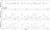 |
Fig. E.1 Phase-folded curves (using the photospheric absorption line period and phase, which is nearly identical to the He II 4686 Å period and phase) for the amplitude of the multi-Gaussian model used to fit the CaII IR lines. Top: NC. Middle: blueshifted BC. Bottom: redshifted BC. There is a marginal amplitude modulation of the BC amplitude. |
In the IR, we also find the CaII 8248 and 8927 Å . Both lines are narrow, very weak and typically noisy, so we cannot obtain much information from them. The 8927 Å line is not detectable in spectra taken at low accretion. The CaII H and K lines in the near-UV have a very different morphology compared to the IR lines. The NC+BC structure is not so evident. The BC has a very strong blueshifted absorption, which is not smooth, but also appears to have some structure. Some redshifted absorption could also be present on certain dates. The blueshifted absorption is clearly correlated with the strength of the accretion rate and likely results from an accretion-powered wind.
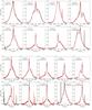 |
Fig. E.2 Some examples of day-to-day modulation of the BC of the Ca II lines (8498 Å line in red, 8662 Å line in black). For each set, phase (φ) and date (d = JD-2 455 000) are given. |
Examining the shape of the BC of the Ca II IR triplet vs. the phase, we find that they are not completely independent. The rapid day-to-day variability observed during outburst (SA12) with strong shifts of the BC peak is evident here when comparing observations taken on consecutive days (Fig. E.2). Selecting only the cases where the BC is strong (≥0.3 over the continuum level) and has a simple shape, we classified the shape of the peak as centred (if the velocity of the BC peak is in the range ±20 km s-1), redshifted (for velocities >20 km s-1), blueshifted (for velocities <−20 km s-1), and double-peak (if the BC has two peaks with normalised height differences <0.2). For each case, we measured both the 8498 Å and 8662 Å lines, and the final classification depends on the averaged result, plus a visual inspection to remove uncertain cases (e.g. those where the top of the BC is flat over a large velocity range). Most of the data points are consistent with either central or blueshifted BC, given that redshifted components tend to fail the strength criterion, often being weaker. Blueshifted BC appear at phases between 0.24−0.5, corresponding to the phases for which the emission lines move from no-shift to blueshifted (Fig. E.3). A KS test shows a probability of 0.9% that the phase correlation is random, which points to a significant correlation between the BC shape and the NC line modulation, and thus to a common dynamical origin. If we assume that the BC is formed in the same accretion structure where the NC comes from, but at a larger distance, the presence of blueshifted BC at these phases would indicate a slightly trailing column, where the material is seen as coming to the observer while the footprint of the accretion column where the NC originates moves from zero to maximum blueshifted velocity with respect to the observer.
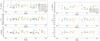 |
Fig. E.3 Shape of the BC (classified as centred, blueshifted, redshifted, and double-peaked, see text) vs. phase. Only data points with strong BC and a clear peak are classified. |
The He I and He II lines
We detect several strong He I lines: at 4471, 5015, 5875, 6678, and 7065 Å. The He I lines differ from the metallic lines in that they do not have a clear NC+BC structure, although this structure was present in the outburst (SA12). They are typically broader than the NC of the metallic lines. This was also observed in outburst (SA12) and has been noted in other stars (Beristain et al. 1998), with the stronger 5875 Å line being up to ~20−30 km s-1, but not broad enough to be regarded as BC. In some cases, a weak BC (which can be blueshifted or redshifted) is also seen. The sharp cut of the 5875 and 6678 Å lines on the blue side could be a blueshifted absorption, a possible wind signature. Unlike the Ca II lines, the He I lines can sometimes become very weak when the accretion rate drops.
The He I lines show the same kind of modulation as is observed in the metallic lines. The amplitude of the modulation is of the same order as the RV amplitude for the photospheric absorption lines, although there is a clear offset between the zero velocities of both. This is a similar effect to what Gahm et al. (2013) observed for the He I lines of RU Lupi. We also observe a mild modulation of the amplitude, similar to what is observed for other metallic lines (Mg I, Fe I, Fe II), but with more noise, perhaps because the line fits are not so well defined owing to the presence of blueshifted absorption components. The potential blueshifted absorption component, which could correspond to a wind, does not show any clear RV variation.
The He II line at 4686 Å is remarkably strong for a low-mass star. Like the He I lines, it has only one component that is broader than the usual metallic NC. The line sometimes appears to have a redshifted tail (perhaps due to an infalling, turbulent component), although it could also be caused by a nearby line (there are many weak and strong lines in the blue and UV part of the spectrum). He II shows the most remarkable and tight RV modulation pattern of all the lines, considering that the line is relatively weak and that it is located in a rather noisy part of the spectrum. Its periodogram shows a very sharp peak at 7.41d, the same as the period observed for the photospheric absorption lines. There is no clear modulation of the line amplitude, although an increase in the blue continuum during episodes of stronger accretion may mask accretion-related flux variations.
The Fe I and Fe II lines
The Fe II lines are among the strongest lines after the typical H, He, and Ca II lines. In particular, multiplet 42 is strong in emission, with good S/N lines at 4923 and 5018 Å . The lines show the NC+BC structure, although in this case the BC is much weaker than for Ca II. The BC shows the same kind of modulation as observed for Ca II. The NC reveals a clear RV modulation with an amplitude comparable to that of the photospheric absorption line, but clearly off-phase. There is also a small modulation of the amplitude, of the same type as described for He II (smaller amplitude at zero velocity) and thus opposite to the amplitude variations of the Ca II IR BC.
The same result is found in other Fe II and Fe I transitions. Other strong iron lines include Fe II at 5362, 5316 Å (this one is very strong and may sometimes have a weak blueshifted absorption), 4549, 4383, 4385 Å and Fe I lines at 5269, 5270 Å. Fe I 5371.49 Å has a nearby unidentified line at about 5369.95 Å, both of which are weak. The Fe I lines in the 3700−4000 Å region are usually noisy and weak. In general, the behaviour of the Fe II and Fe I lines is similar. Their BC show bulk velocity shifts that are consistent with those of Ca II. Their NC have clear RV modulations, although some of the lines are too weak or too noisy to find a clear pattern in them. Different lines have different zero-point RV and amplitudes.
The Mg I multiplet at 5167, 5172, 5183 Å
Several Mg I lines are also detected in the quiescence spectra, among them the multiplet at 5167, 5172, and 5183 Å. The lines are strong and mostly narrow, with BC that are usually faint and noisy but become stronger when the BC of Ca II IR gets stronger. They show similar velocity patterns to the Ca II and Fe I, Fe II lines. The NC shows the usual RV modulation observed in Fe I and Fe II, opposite to the photospheric lines RV, and the same variations in amplitude vs. phase, with the lines getting stronger at the maximum blueshifted and redshifted velocity. As also occurs for the Ca II lines, there is a small offset in velocity between the 5167 Å line and the other two, although in this case contamination by a nearby strong Fe I line cannot be excluded.
The O I 7774 triplet and 8446 Å line
The O I triplet around 7774 Å and 8446 Å are also very strong in EX Lupi. The 8446 Å complex, being a blended triplet itself, has a complex structure, very extended and rather weak or undetectable at low accretion rates. It does not have a clear NC, although it is narrower in the centre and has very extended BC wings (up to ±150 km s-1) that changes from blueshifted to redshifted following the patterns observed for Ca II. The line could sometimes have a weak redshifted absorption, although owing to the low S/N and the redshifted emission of the BC, it is not evident. Because of the complexity of the line, it is not possible to study its RV.
The OI 7774 triplet is much stronger and is always detected. The 7772 Å line is very strong and narrow and easy to fit, giving very good results. Having a typical width around 14−16 km s-1, it also shows a BC when the accretion rate increases. The behaviour of the BC is hard to establish because of the presence of the other triplet lines. Fitting the two weaker lines is often a problem owing to the contamination by the BC of the strong 7772 Å line. The 7772 Å line displays the same kind of RV modulation as the rest of metallic lines, and has the same weak modulation of the line amplitude. Its width could also be modulated, becoming thinner when the amplitude decreases, but this is very uncertain owing to the complexity of the continuum around the triplet where the BC of all three lines are blended.
Other lines
As mentioned in SA12, EX Lupi in quiescence shows more than 200 emission lines, of which at present we have only investigated the strongest ones. Other lines include neutral elements (such as Mn I and Cr I), which are weaker than the mentioned Fe I and Mg I lines, and other ionised species (mostly Si II and Ti II). Table A.3 contains the list of strong, unblended lines identified in the spectra.
The Cr I 4254 and 4274 Å lines are relatively strong and narrow (~8−10 km s-1), although they are partially affected by photospheric absorption lines. Although they are noisier, they show the same RV and amplitude modulation as the other metallic lines.
The Si II 6347 and 6371 Å lines are also relatively strong. The 6347 Å line sometimes shows evidence for a BC with the usual velocity pattern, although the lines become nearly undetectable when the accretion rate decreases. Both lines show the RV modulation observed for the rest of metallic lines, although the amplitude of the modulation is slightly lower than observed for the photospheric absorption lines.
The Ti II lines at 4300, 4302, and 4307 Å are also detected, despite the poor S/N of the spectra in this area. They are narrow (8−12 km s-1), although one of the spectra shows a hint of a BC. Despite the high noise level, they show the usual RV modulation with a peak-to-peak amplitude of about 6 km s-1 and the usual sinusoidal modulation, although in blue and UV lines the amplitude can easily be distorted by poor continuum determination when the S/N is low.
Other lines such as Mn I at 4030 Å are very faint, so any attempt to fit and extract them is noise-dominated.
The Ca II H line is contaminated by Hϵ.
Considering the consistent opacity-related shift observed between the two Ca II IR lines, we should be able to detect any modulation with amplitude at the ~0.5 km s-1 level, if there is any.
This may not hold as we move away from the object. From the Vz of the lines, if infall is assumed, the lines would be produced very close to the stellar surface, so d ≪ R∗.
For instance, the Ca II IR BC are not entirely symmetric but deviate from pure Gaussian profiles.
The region where the NC are produced is expected to be very small compared to the stellar radius, which means that the nearly solid-body rotation would not need to be extended over a large vertical structure.
In the presence of a strong magnetic field near the stellar photosphere, the infall is probably caused by downward motions along the magnetic field structure that corotates with the star.
Acknowledgments
We thank the La Silla observers, specially J. Setiawan and A. Müller, for collecting the spectra. We also thank the anonymous referee for his/her valuable comments that helped clarify this paper, A. Mortier for her comments on spot-related rotational modulations, and A. Scholz for his comments on accretion-related variability. This research made use of Astropy, a community-developed core Python package for Astronomy (Astropy Collaboration, 2013). A.S.A. and M.F. acknowledge support from the Spanish “Proyectos de investigación no orientada” project number AYA2012-35008. A.K. is partly supported by the Momentum grant of the MTA CSTK Lendület Disk Research Group. P.Á. acknowledges support from the Hungarian Research Grant OTKA 101393.
References
- Ábrahám, P., Juhász, A., Dullemond, C. P., et al. 2009, Nature, 459, 224 [NASA ADS] [CrossRef] [PubMed] [Google Scholar]
- Alcalá, J. M., Natta, A., Manara, C. F., et al. 2014, A&A, 561, A2 [NASA ADS] [CrossRef] [EDP Sciences] [Google Scholar]
- Alencar, S., Johns-Krull, C., & Basri, G. 2001, AJ, 122, 3335 [NASA ADS] [CrossRef] [Google Scholar]
- Andrews, S., & Williams, J. 2007, ApJ, 671, 1800 [CrossRef] [Google Scholar]
- Ardila, D. R., Herczeg, G. J., Gregory, S. G., et al. 2013, ApJS, 207, 1 [NASA ADS] [CrossRef] [EDP Sciences] [Google Scholar]
- Appenzeller, I., & Wagner, S. 1989, A&A, 225, 432 [NASA ADS] [Google Scholar]
- Appenzeller, I., Oestreicher, R., Schiffer, J. G., Egge, K. E., & Pettersen, B. R. 1983, A&A, 118, 75 [NASA ADS] [Google Scholar]
- Appenzeller, I., Jetter, R., & Jankovics, I. 1986, A&AS, 64, 65 [NASA ADS] [Google Scholar]
- Argiroffi, C., Flaccomio, E., Bouvier, J., et al. 2011, A&A, 530, A1 [NASA ADS] [CrossRef] [EDP Sciences] [Google Scholar]
- Argiroffi, C., Maggio, A., Montmerle, T., et al. 2012, ApJ, 752, 100 [NASA ADS] [CrossRef] [Google Scholar]
- Artymowicz, P., & Lubow, S. H. 1996, ApJ, 467, L77 [NASA ADS] [CrossRef] [Google Scholar]
- Aspin, C., Reipurth, B., Herczeg, G. J., & Capak, P. 2010, ApJ, 719, L50 [NASA ADS] [CrossRef] [Google Scholar]
- Banzatti, A., Pontoppidan, K. M., Bruderer, S., Muzerolle, J., & Meyer, M. R. 2015, ApJ, 798, LL16 [Google Scholar]
- Beristain, G., Edwards, S., & Kwan, J. 1998, ApJ, 499, 828 [NASA ADS] [CrossRef] [Google Scholar]
- Beristain, G., Edwards, S., & Kwan, J. 2001, ApJ, 551, 1037 [NASA ADS] [CrossRef] [Google Scholar]
- Brickhouse, N. S., Cranmer, S. R., Dupree, A. K., Luna, G. J. M., & Wolk, S. 2010, ApJ, 710, 1835 [NASA ADS] [CrossRef] [Google Scholar]
- Brickhouse, N. S., Cranmer, S. R., Dupree, A. K., et al. 2012, ApJ, 760, L21 [NASA ADS] [CrossRef] [Google Scholar]
- Brown, B. P., Miesch, M. S., Browning, M. K., Brun, A. S., & Toomre, J. 2011, ApJ, 731, 69 [NASA ADS] [CrossRef] [Google Scholar]
- Costigan, G., Vink, J. S., Scholz, A., Ray, T., & Testi, L. 2014, MNRAS, 440, 3444 [NASA ADS] [CrossRef] [Google Scholar]
- D’Alessio, P., Calvet, N., & Hartmann, L. 2001, ApJ, 553, 321 [NASA ADS] [CrossRef] [Google Scholar]
- D’Alessio, P., Calvet, N., Hartmann, L., Franco-Hernández, R., & Servín, H. 2006, ApJ, 638, 314 [NASA ADS] [CrossRef] [Google Scholar]
- Dodin, A. V., & Lamzin, S. A. 2012, Astron. Lett., 38, 649 [NASA ADS] [CrossRef] [Google Scholar]
- Dodin, A. V., Lamzin, S. A., & Chuntonov, G. A. 2012, Astron. Lett., 38, 167 [NASA ADS] [CrossRef] [Google Scholar]
- Donati, J.-F., Collier Cameron, A., Semel, M., et al. 2003, MNRAS, 345, 1145 [NASA ADS] [CrossRef] [Google Scholar]
- Dullemond, C., & Dominik, C. 2004, A&A, 417, 159 [NASA ADS] [CrossRef] [EDP Sciences] [Google Scholar]
- Dumusque, X., Boisse, I., & Santos, N. C. 2014, ApJ, 796, 132 [NASA ADS] [CrossRef] [Google Scholar]
- Dupree, A. K., Brickhouse, N. S., Cranmer, S. R., et al. 2012, ApJ, 750, 73 [NASA ADS] [CrossRef] [Google Scholar]
- Edwards, S., Cabrit, S., Strom, S. E., et al. 1987, ApJ, 321, 473 [NASA ADS] [CrossRef] [Google Scholar]
- Edwards, S., Hartigan, P., Ghandour, L., & Andrulis, C. 1994, AJ, 108, 1056 [NASA ADS] [CrossRef] [Google Scholar]
- Fang, M., van Boekel, R., Wang, W., et al. 2009, A&A, 504, 461 [NASA ADS] [CrossRef] [EDP Sciences] [Google Scholar]
- Flaccomio, E., Micela, G., Sciortino, S., et al. 2005, ApJS, 160, 450 [NASA ADS] [CrossRef] [Google Scholar]
- Gahm, G. F., Petrov, P. P., Duemmler, R., Gameiro, J. F., & Lago, M. T. V. T. 1999, A&A, 352, L95 [NASA ADS] [Google Scholar]
- Gahm, G. F., Stempels, H. C., Walter, F. M., Petrov, P. P., & Herczeg, G. J. 2013, A&A, 560, A57 [NASA ADS] [CrossRef] [EDP Sciences] [Google Scholar]
- Goto, M., Regály, Z., Dullemond, C. P., et al. 2011, ApJ, 728, 5 [NASA ADS] [CrossRef] [Google Scholar]
- Gregory, S. G., Holzwarth, V. R., Donati, J.-F., et al. 2014, IAU Symp., 302, 44 [NASA ADS] [Google Scholar]
- Grinin, V. P., & Mitskevich, A. S. 1988, Izv. Krym. Astrofiz. Obs., 78, 28 [NASA ADS] [Google Scholar]
- Grosso, N., Hamaguchi, K., Kastner, J. H., Richmond, M. W., & Weintraub, D. A. 2010, A&A, 522, A56 [NASA ADS] [CrossRef] [EDP Sciences] [Google Scholar]
- Gullbring, E., Hartmann, L., Briceño, C., & Calvet, N. 1998, ApJ, 492, 323 [NASA ADS] [CrossRef] [Google Scholar]
- Hamann, F., & Persson, S. E. 1992a, ApJS, 82, 247 [NASA ADS] [CrossRef] [Google Scholar]
- Hartigan, P., Hartmann, L., Kenyon, S. J., Strom, S. E., & Skrutskie, M. F. 1990, ApJ, 354, L25 [NASA ADS] [CrossRef] [Google Scholar]
- Hartmann, L., Hewett, R., & Calvet, N. 1994, ApJ, 426, 669 [NASA ADS] [CrossRef] [Google Scholar]
- Herbig, G. 1950, PASP, 62, 211 [NASA ADS] [CrossRef] [Google Scholar]
- Herbig, G. 1977, ApJ, 214, 747 [NASA ADS] [CrossRef] [Google Scholar]
- Herbig, G. 2007, AJ, 133, 2679 [Google Scholar]
- Herbig, G. 2008, AJ, 135, 637 [NASA ADS] [CrossRef] [Google Scholar]
- Herbig, G. H. 1989, ESO Conf. Workshop Proc., 33, 233 [Google Scholar]
- Herbig, G., Aspin, C., Gilmore, A., Imhoff, C., Jones, A. 2001, PASP, 113, 1547 [NASA ADS] [CrossRef] [Google Scholar]
- Holoien, T. W.-S., Prieto, J. L., Stanek, K. Z., et al. 2014, ApJ, 785, LL35 [Google Scholar]
- Horne, J. H., & Baliunas, S. L. 1986, ApJ, 302, 757 [NASA ADS] [CrossRef] [Google Scholar]
- Ingleby, L., Calvet, N., Herczeg, G., et al. 2013, ApJ, 767, 112 [NASA ADS] [CrossRef] [Google Scholar]
- Jeffers, S. V., Barnes, J. R., Jones, H. R. A., et al. 2014, MNRAS, 438, 2717 [NASA ADS] [CrossRef] [Google Scholar]
- Johns-Krull, C. M., Chen, W., Valenti, J. A., et al. 2013, ApJ, 765, 11 [NASA ADS] [CrossRef] [Google Scholar]
- Johnstone, C. P., Jardine, M., Gregory, S. G., Donati, J.-F., & Hussain, G. 2014, MNRAS, 437, 3202 [NASA ADS] [CrossRef] [Google Scholar]
- Jones, A. 2008,Central Bureau Electronic Telegrams, 1217, 1 [Google Scholar]
- Juhász, A., Dullemond, C. P., van Boekel, R., et al. 2012, ApJ, 744, 118 [NASA ADS] [CrossRef] [Google Scholar]
- Kaufer, A., Stahl, O., Tubbesing, S., et al. 1999, The Messenger, 95, 8 [Google Scholar]
- Kelleher, D. E., Mohr, P. J., Martin, W. C., et al. 1999, Proc. SPIE, 3818, 170 [Google Scholar]
- Kóspál, Á., Nemeth, P., Abraham, P., et al. 2008, IBVS, 5819, 1 [NASA ADS] [Google Scholar]
- Kóspál, Á., Ábrahám, P., Goto, M., et al. 2011, ApJ, 736, 72 [NASA ADS] [CrossRef] [Google Scholar]
- Kóspál, Á., Mohler-Fischer, M., Sicilia-Aguilar, A., et al. 2014, A&A, 561, A61 [NASA ADS] [CrossRef] [EDP Sciences] [Google Scholar]
- Kurosawa, R., & Romanova, M. M. 2013, MNRAS, 431, 2673 [NASA ADS] [CrossRef] [Google Scholar]
- Lago, M. T. V. T., & Gameiro, J. F. 1998, MNRAS, 294, 272 [NASA ADS] [CrossRef] [Google Scholar]
- Lehmann, T., Reipurth, B., & Brandner, W. 1995, A&A, 300, L9 [NASA ADS] [Google Scholar]
- Luridiana, V., Morisset, C., & Shaw, R. A. 2012, IAU Symp., 283, 422 [NASA ADS] [Google Scholar]
- Marsden, S. C., Jeffers, S. V., Donati, J.-F., et al. 2010, IAU Symp., 264, 130 [NASA ADS] [Google Scholar]
- Martin, W. C., & Wiese, W. L. 1999, National Institute of Standards and Technology, Atomic, web version of Chapter 10 of Molecular, and Optical Physics handbook, ed. G. W. F. Drake (Woodbury, NY: AIP Press) [Google Scholar]
- Mayor, M., Pepe, F., Queloz, D., et al. 2003, The Messenger, 114, 20 [NASA ADS] [Google Scholar]
- McLaughlin, D. B. 1946, AJ, 52, 109 [NASA ADS] [CrossRef] [Google Scholar]
- Mihalas, D. 1978, Stellar Atmospheres (San Francisco: W. H. Freeman and Co.) [Google Scholar]
- Mora, A., Natta, A., Eiroa, C., et al. 2002, A&A, 393, 259 [NASA ADS] [CrossRef] [EDP Sciences] [Google Scholar]
- Mora, A., Eiroa, C., Natta, A., et al. 2004, A&A, 419, 225 [NASA ADS] [CrossRef] [EDP Sciences] [Google Scholar]
- Morin, J., Donati, J.-F., Petit, P., et al. 2010, MNRAS, 407, 2269 [NASA ADS] [CrossRef] [MathSciNet] [Google Scholar]
- Müller, A., Roccatagliata, V., Henning, T., et al. 2013, A&A, 556, A3 [NASA ADS] [CrossRef] [EDP Sciences] [Google Scholar]
- Muzerolle, J., Hartmann, L., & Calvet, N. 1998, AJ, 116, 455 [NASA ADS] [CrossRef] [Google Scholar]
- Muzerolle, J., Calvet, N., & Hartmann, L. 2001, ApJ, 550, 944 [NASA ADS] [CrossRef] [Google Scholar]
- Natta, A., Testi, L., Neri, R., Schepherd, D., & Wilner, D. 2004, A&A, 416, 179 [NASA ADS] [CrossRef] [EDP Sciences] [Google Scholar]
- Orlando, S., Sacco, G. G., Argiroffi, C., et al. 2010, A&A, 510, A71 [NASA ADS] [CrossRef] [EDP Sciences] [Google Scholar]
- Orlando, S., Bonito, R., Argiroffi, C., et al. 2013, A&A, 559, A127 [NASA ADS] [CrossRef] [EDP Sciences] [Google Scholar]
- Patten, B. M. 1994, IBVS, 4049, 1 [NASA ADS] [Google Scholar]
- Petrov, P. P., Pelt, J., & Tuominen, I. 2001, A&A, 375, 977 [NASA ADS] [CrossRef] [EDP Sciences] [Google Scholar]
- Petrov, P. P., Gahm, G. F., Herczeg, G. J., Stempels, H. C., & Walter, F. M. 2014, A&A, 568, L10 [NASA ADS] [CrossRef] [EDP Sciences] [Google Scholar]
- Ralchenko, Yu., Kramida, A. E., Reader, J., & NIST ASD Team 2010, NIST Atomic Spectra Database ver. 4.0.1, http://physics.nist.gov/asd [Google Scholar]
- Robitaille, T. P., et al. (Astropy Collaboration) 2013, A&A, 558, A33 [NASA ADS] [CrossRef] [EDP Sciences] [Google Scholar]
- Romanova, M. M., Ustyugova, G. V., Koldoba, A. V., & Lovelace, R. V. E. 2004, ApJ, 610, 920 [NASA ADS] [CrossRef] [Google Scholar]
- Romanova, M. M., Ustyugova, G. V., Koldoba, A. V., & Lovelace, R. V. E. 2011, MNRAS, 416, 416 [NASA ADS] [Google Scholar]
- Scargle, J. D. 1982, ApJ, 263, 835 [NASA ADS] [CrossRef] [Google Scholar]
- Shine, R. A., & Linsky, J. L. 1974, Sol. Phys., 39, 49 [NASA ADS] [CrossRef] [Google Scholar]
- Sicilia-Aguilar, A., Henning, Th., Hartmann, L. 2010, ApJ, 710, 597 [NASA ADS] [CrossRef] [Google Scholar]
- Sicilia-Aguilar, A., Kóspál, Á., Setiawan, J., et al. 2012, A&A, 544, A93 [NASA ADS] [CrossRef] [EDP Sciences] [Google Scholar]
- Sipos, N., Ábrahám, P., Acosta-Pulido, J., et al. 2009, A&A, 507, 881 [NASA ADS] [CrossRef] [EDP Sciences] [Google Scholar]
- Stempels, H. C., Gahm, G. F., & Petrov, P. P. 2007, A&A, 461, 253 [NASA ADS] [CrossRef] [EDP Sciences] [Google Scholar]
- Symington, N. H., Harries, T. J., Kurosawa, R., & Naylor, T. 2005, MNRAS, 358, 977 [NASA ADS] [CrossRef] [Google Scholar]
- Zechmeister, M., & Kuerster, M. 2009, A&A, 496, 577 [NASA ADS] [CrossRef] [EDP Sciences] [Google Scholar]
All Tables
Non-blended, narrow emission lines observed in EX Lupi, based on line identifications by SA12, and using the atomic constants from the NIST database.
Cross-correlation coefficients for the Gaussian fits to the CaII 8498 and 8662Å lines.
All Figures
|
Fig. 1 Hα and Hβ line profile variability (left) and autocorrelation matrix (right). The pixel-by-pixel median of the line is shown as a thick blue line. The pixel-by-pixel rms is shown as the thick black line and shaded area. The zero velocities/wavelengths of the lines are marked as dashed vertical lines. The correlation coefficient (estimated as a Spearman rank correlation with value r and false alarm probability p) is shown on the right in the colour scheme, with the black contours marking the high significance (p> 10-5) areas with r = 0.6,0.7,0.8,0.9. |
| In the text | |
|
Fig. 2 Same as Fig. 1 for the Ca II K (top) and 8498 Å (bottom) lines. The pixel-by-pixel median of the line is shown as a thick blue line. The pixel-by-pixel rms is shown as the thick black line and shaded area. The zero velocities/wavelengths of the lines are marked as dashed vertical lines. The correlation coefficient (estimated as a Spearman rank correlation with value r and false alarm probability p) is shown on the right in the colour scheme, with the black contours marking the high significance (p> 10-5) areas with r = 0.6,0.7,0.8,0.9. |
| In the text | |
|
Fig. 3 Pixel-by-pixel velocity cross-correlations between different lines. From top to bottom, left to right: Ca II 8498 vs. 8662 Å, Ca II K vs. Ca II 8498 Å, Ca II 8498 Å vs. Hα, Ca II 8222 Å vs. He I 5875 Å, Hα vs. He I 5875 Å, and Ca II 8498 Å vs. Hβ. The correlation coefficient (estimated as a Spearman rank correlation with value r and false alarm probability p) is shown on the right in the colour scheme, with the contours marking the high significance (p> 10-5) areas with r = 0.6,0.7,0.8,0.9. |
| In the text | |
|
Fig. 4 Some of the multi-Gaussian fits for one of the dates (JD 2 455 674.82443). The normalised, continuum-subtracted observed spectra are displayed as thick black lines. Individual Gaussian components are plotted as thin lines (colours: green, red, blue, cyan). The combined fit is plotted as a magenta thick line. The zero velocities of the central line are also marked with a vertical dotted line. The plots are labelled with the line(s) elements and wavelength. Note that the very complex shape of the continuum around the Fe I 5269/70 Å lines is better fitted by two strong Gaussians, one in emission and the other in absorption (partly out of the figure). These BC have no physical meaning/interpretation, but allow us to extract properly the strong NC of both lines. |
| In the text | |
|
Fig. 5 Some examples of GLS periodograms for different lines. The 7.41d period (marked as a blue dashed line) becomes increasingly significant as we move to lines with higher excitation potentials. The FAP are marked as dotted horizontal lines and labelled accordingly. The situation observed for Mg I is typical of the rest of metallic lines labelled as having several peaks. |
| In the text | |
|
Fig. 6 Phase-folded curves (using the photospheric absorption line period and phase, which is nearly identical to the He II 4686 Å line period and phase) for several of the observed NC of lines. We note that two 7.417d periods are plotted for clarity. The dotted line represents the RV curve measured for the photospheric absorption lines (K14). |
| In the text | |
|
Fig. 7 Scheme of the effect of a hot spot that rotates with the star affects the photospheric absorption lines. In A) we show the different parts of the stellar photosphere that produce the photospheric absorption lines. B) shows how the line is affected when a hot spot is included. When the absorption deficit associated with the spot appears blueshifted, the centre of the photospheric lines seems to move towards the red. When the spot appears redshifted, the centre of the absorption line appears shifted towards the blue. Small emission lines are visible within some of the photospheric absorption lines, tracking the local rotational velocity of the part of the stellar surface where the line originates. Non-photospheric lines or lines that are particularly strong on the spot could appear simply as emission lines over the continuum, without any underlying absorption. |
| In the text | |
|
Fig. 8 Cartoon of a star with an accretion column that is visible at all times due to the stellar inclination and whose emission lines suffer Doppler shift as the star rotates (the observer is located perpendicular to the plane of the paper). The blue (red) column shows the position at which the lines originated in it would appear blueshifted (redshifted) to an observer looking from out of the page. The hashed areas mark the shock region. We suggest that the observed narrow emission lines are produced in the post-shock area, which is stratified in density and temperature. Lines produced in the shock region (He II, requiring very hot and dense conditions) originate in a nearly flat structure, so their periodic signatures are much stronger and less messy than other lines produced in the extended, infalling post-shock region. The BC is produced in the accretion column before the pre-shock region, showing higher velocity offsets as they rotate with/around the star. Not to scale: we note that the shock region is at a very small distance over the photosphere, compared to the stellar radius. |
| In the text | |
|
Fig. 9 Results of our toy model for the RV signatures (upper panel), and bisector velocity shift (BVS) and curvature (BC; lower panels). It shows the kind of RV modulations that can be induced on a photospheric absorption line by an emission component (broader than the absorption line) that shows a rotational modulation. “P” denotes the peak value of an emission component with a Voigt profile with Gaussian width σ and Lorentzian contribution γ. “Cont” marks the classical veiling continuum added to the model. “A” denotes the RV amplitude of the emission line (maximum RV offset for a sinusoidal modulation), and “RS” is the zero-point redshift of the line. The dashed box shows the values of the bisector velocity as measured by K14, which are similar to those derived from the toy model. Although there is a slight BVS slope, the typical errors at this level can make it very hard to distinguish. |
| In the text | |
|
Fig. 10 Attempt to reproduce the median EX Lupi spectrum (black line, with standard deviation per pixel marked in grey) by using a rotationally broadened standard veiled by a continuum emission (magenta). The difference between the observed and veiled spectra is shown in pink. A constant veiling cannot reproduce the depths of all lines, even if we only consider a very small wavelength range. The differences are too large to be explained by the standard deviation or time variation observed between the different spectra. |
| In the text | |
|
Fig. 11 Toy model for the narrow emission lines, obtained by considering an electron density 1013 cm-3 and three different temperatures along the accretion column (8000, 10 000, 23 000 K). The rotationally broadened standard star spectrum is shown in grey, and the individual lines are shown in various colours. The final model, including a constant veiling, is obtained by summing all three components. |
| In the text | |
|
Fig. C.1 Line fit parameters for the NC of the Ca II IR (left) and He II lines (right), colour-coded according to their accretion rate (see text). The upper panel shows the RV of the NC line (VNC), the middle panel the amplitude of the NC line (ANC), and the bottom panel the Gaussian width (σNC). There is no evident modulation of the RV with the accretion rate, and only the line width for the Ca II NC seems to be higher for the higher accretion rates, although this could be also an effect of the presence of a stronger underlying BC. The signatures observed in the NC are thus very robust with respect to variations of the accretion rate within one order of magnitude. |
| In the text | |
|
Fig. E.1 Phase-folded curves (using the photospheric absorption line period and phase, which is nearly identical to the He II 4686 Å period and phase) for the amplitude of the multi-Gaussian model used to fit the CaII IR lines. Top: NC. Middle: blueshifted BC. Bottom: redshifted BC. There is a marginal amplitude modulation of the BC amplitude. |
| In the text | |
|
Fig. E.2 Some examples of day-to-day modulation of the BC of the Ca II lines (8498 Å line in red, 8662 Å line in black). For each set, phase (φ) and date (d = JD-2 455 000) are given. |
| In the text | |
|
Fig. E.3 Shape of the BC (classified as centred, blueshifted, redshifted, and double-peaked, see text) vs. phase. Only data points with strong BC and a clear peak are classified. |
| In the text | |
Current usage metrics show cumulative count of Article Views (full-text article views including HTML views, PDF and ePub downloads, according to the available data) and Abstracts Views on Vision4Press platform.
Data correspond to usage on the plateform after 2015. The current usage metrics is available 48-96 hours after online publication and is updated daily on week days.
Initial download of the metrics may take a while.