| Issue |
A&A
Volume 580, August 2015
|
|
|---|---|---|
| Article Number | A54 | |
| Number of page(s) | 15 | |
| Section | Extragalactic astronomy | |
| DOI | https://doi.org/10.1051/0004-6361/201525630 | |
| Published online | 30 July 2015 | |
Velocity resolved [C ii], [C i], and CO observations of the N159 star-forming region in the Large Magellanic Cloud: a complex velocity structure and variation of the column densities
1 I. Physikalisches Institut der Universität zu Köln, Zülpicher Straße 77, 50937 Köln, Germany
e-mail: This email address is being protected from spambots. You need JavaScript enabled to view it.
2 Max-Planck-Institut für Radioastronomie, Auf dem Hügel 69, 53121 Bonn, Germany
Received: 9 January 2015
Accepted: 23 April 2015
Abstract
Context. The [C ii] 158 μm fine structure line is one of the dominant cooling lines in star-forming active regions. Together with models of photon-dominated regions, the data is used to constrain the physical properties of the emitting regions, such as the density and the radiation field strength. According to the modeling, the [C ii] 158 μm line integrated intensity compared to the CO emission is expected to be stronger in lower metallicity environments owing to lower dust shielding of the UV radiation, a trend that is also shown by spectral-unresolved observations. In the commonly assumed clumpy UV-penetrated cloud scenario, the models predict a [C ii] line profile similar to that of CO. However, recent spectral-resolved observations by Herschel/HIFI and SOFIA/GREAT (as well as the observations presented here) show that the velocity resolved line profile of the [C ii] emission is often very different from that of CO lines, indicating a more complex origin of the line emission including the dynamics of the source region.
Aims. The Large Magellanic Cloud (LMC) provides an excellent opportunity to study in great detail the physics of the interstellar medium (ISM) in a low-metallicity environment by spatially resolving individual star-forming regions. The aim of our study is to investigate the physical properties of the star-forming ISM in the LMC by separating the origin of the emission lines spatially and spectrally. In this paper, we focus on the spectral characteristics and the origin of the emission lines, and the phases of carbon-bearing species in the N159 star-forming region in the LMC.
Methods. We mapped a 4′ × (3′–4′) region in N159 in [C ii] 158 μm and [N ii] 205 μm with the GREAT instrument on board SOFIA. We also observed CO(3–2), (4–3), (6–5), 13CO(3–2), and [C i] 3P1–3P0 and 3P2–3P1 with APEX. All spectra are velocity resolved.
Results. The emission of all transitions observed shows a large variation in the line profiles across the map and in particular between the different species. At most positions the [C ii] emission line profile is substantially wider than that of CO and [C i]. We estimated the fraction of the [C ii] integrated line emission that cannot be fitted by the CO line profile to be 20% around the CO cores, and up to 50% at the area between the cores, indicating a gas component that has a much larger velocity dispersion than the ones probed by the CO and [C i] emission. We derived the relative contribution from C+, C, and CO to the column density in each velocity bin. The result clearly shows that the contribution from C+ dominates the velocity range far from the velocities traced by the dense molecular gas. Spatially, the region located between the CO cores of N159 W and E has a higher fraction of C+ over the whole velocity range. We estimate the contribution of the ionized gas to the [C ii] emission using the ratio to the [N ii] emission, and find that the ionized gas contributes ≤19% to the [C ii] emission at its peak position, and ≤15% over the whole observed region. Using the integrated line intensities, we present the spatial distribution of I[CII]/IFIR.
Conclusions. This study demonstrates that the [C ii] emission in the LMC N159 region shows significantly different velocity profiles from that of CO and [C i] emissions, emphasizing the importance of velocity resolved observations in order to distinguish different cloud components.
Key words: ISM: lines and bands / ISM: kinematics and dynamics / Magellanic Clouds / ISM: individual objects: N159
© ESO, 2015
1. Introduction
The [C ii] 158 μm fine structure transition is one of the dominant cooling lines in photon-dominated regions (PDRs; Tielens & Hollenbach 1985; Sternberg & Dalgarno 1995), and it is used to constrain their physical properties. Because of its strength, it also has a great potential for tracing star formation activity in external galaxies and for estimating the star formation rate (de Looze et al. 2011, and references therein). On the other hand, changes in the metallicity affect the abundance of the major coolants including carbon, the electron densities in PDRs, the dust abundance that determines the UV penetration, the photoelectric heating rate, and the H2 formation rate, resulting in a larger C+ layer in the low-metallicity environment (Bolatto et al. 1999; Röllig et al. 2006). This metallicity dependence is also shown observationally as a two-order-of-magnitude difference in the intensity ratio of [C ii] and CO among galaxies with different metallicities (Mochizuki et al. 1994; Poglitsch et al. 1995; Israel et al. 1996; Madden et al. 1997, 2011). In order to understand the extragalactic [C ii] emission, which is the superimposed emission from different physical environments, our interpretation needs to bridge detailed Galactic studies to observations of marginally or non-spatially resolved external galaxies. The Large Magellanic Cloud (LMC) is one of the most important targets because its different metallicity from our Galaxy (~1/3 of solar; Carrera et al. 2008) enables us to investigate the influence of the metallicity on the thermal balance and chemical composition in the ISM, and its proximity (50 kpc as a median distance of 729 references; NASA/IPAAC Extragalactic Database) allows spatially resolved studies of the large star-forming regions visible in the LMC.
In most cases, integrated line intensities of [C ii] and CO emission are used as diagnostics in external galaxies. However, velocity resolved mapping observations of the [C ii] emission in Galactic regions have recently been made with the Heterodyne Instrument for the Far-Infrared (HIFI) on Herschel and are being made with the German REceiver for Astronomy at Terahertz Frequencies (GREAT) on board the Stratospheric Observatory for Infrared Astronomy (SOFIA), and they show complex line profiles of the [C ii] emission, typically substantially wider than expected from the [C i] and low- or mid-J CO emission profiles. The velocity information is thus essential in order to identify the origin of the [C ii] emission (Pérez-Beaupuits et al. 2012; Carlhoff 2013), and the significant difference in the velocity profile of the [C ii] emission from the low- or mid-J CO emission indicates that a substantial fraction of the [C ii] emission is accelerated relative to the quiescent material, e.g., it undergoes ablation or is blown off (Dedes et al. 2010; Mookerjea et al. 2012; Okada et al. 2012; Schneider et al. 2012; Simon et al. 2012; Pilleri et al. 2012). These results emphasize the need of velocity resolved observations to distinguish different velocity components with their different physical conditions.
Before the HIFI and GREAT observations only the pioneering heterodyne observations from the Kuiper Airborne Observatory (KAO) were available. Boreiko & Betz (1991) observed 17 locations in the LMC and showed that the [C ii] emission is approximately 50% wider than the CO(2–1) line. However, investigating its spatial variation and the line profile in detail requires mapping observations and a higher signal-to-noise ratio (S/N) than was available at that time; HIFI provided the necessary higher S/N, but the mapping ability was still limited and allowed only a few strip maps to be observed across a few prominent regions in the LMC.
Since CO lines are observable from the ground, more velocity resolved observations have been done for them. In the N159 star-forming region, which we focus on in this paper, physical properties of the clouds have been studied using low-J CO mapping observations (Johansson et al. 1998; Minamidani et al. 2008, 2011; Mizuno et al. 2010) or using single point observations of CO(4–3), CO(7–6), and [C i] 3P1–3P0 and 3P2–3P1 emissions (Pineda et al. 2008), but detailed line profiles have not been discussed. Bolatto et al. (2000) present a large-scale map and velocity resolved spectra of [C i] 3P1–3P0, but with a spatial resolution of only 4′, which is insufficient to resolve the individual source components spatially.
The aim of our GREAT core project on the LMC and Small Magellanic Cloud (SMC) is to study physical properties by distinguishing the origin of the emission lines using velocity profiles in active regions in the LMC and SMC and to investigate the effect of the low-metallicity environment on the properties and evolution of the interstellar medium (ISM). In this paper, we present observations in N159, focusing on the velocity profiles and the origin of the emission lines, and present the column density ratio between C+, C, and CO using simple assumptions. We do not deal with any elaborate PDR modeling or with the metallicity effects. A full PDR model analysis will be presented in a follow-up paper (Okada et al., in prep.). N159 is located south of 30 Dor as a part of the molecular ridge (Cohen et al. 1988; Mizuno et al. 2001). Three CO cores are identified (N159 W, E, and S; Johansson et al. 1998). N159 S shows no evidence of star-forming activity, while W and E possess O-type stars and H ii regions, where massive stars formed a few Myr ago (Chen et al. 2010). The results of 30 Dor and N66 in the SMC are presented in a separate paper (Requena et al. in prep.).
2. Observations and data reduction
2.1. [C II] 158 μm and [N II] 205 μm observations with SOFIA/GREAT
Observation parameters.
We mapped 4′ × (3′–4′) in the N159 star-forming region in the LMC, observing the [C ii] emission at 1900.5369 GHz (158 μm) using the German REceiver for Astronomy at Terahertz Frequencies (GREAT1; Heyminck et al. 2012) on board the Stratospheric Observatory for Infrared Astronomy (SOFIA; Young et al. 2012) in July 2013, as part of the open time and guaranteed time in cycle 1 observations. Observations were performed during four flights of SOFIA’s first southern deployment to New Zealand and the L2 channel was tuned to [C ii]. During the first two flights, we observed in parallel [N ii] 205 μm with the L1 channel. The observations were made in total-power on-the-fly (OTF) mode, with 0.5 to 2 s integration time per dump, at 6′′ step size. The total flight time for N159 observations was about 4 h and the total integration time on source was about 1 h. The OFF position for the observations was located southwest of the observed region (05h38m53 3, −69°46′29′′ (J2000)), which is the same OFF position used in Pineda et al. (2008).
Pointing on SOFIA is done via a combination of fast inertial gyro stabilization of the telescope and regular corrections on the optical guide cameras. Experience shows that pointing and tracking is better than 2 arcsecs. The alignment between the telescope optical axis, i.e., the guide cameras, and the boresight of the GREAT instrument is checked and verified at the beginning of each observing campaign after installation of the GREAT instrument by observing a suitable planet, and was 1.5 arcsecs.
The data from the extended bandwidth Fourier transform spectrometer (XFFTS; 2.5 GHz bandwidth with 44 kHz resolution) were calibrated by the standard GREAT pipeline (Guan et al. 2012). Details of the observations are listed in Table 1. A polynomial of second order was used to fit the baseline. We checked the results obtained with polynomials of first to fourth order as a baseline, and found that a first-order polynomial results in higher baseline noise, fourth-order polynomials introduce artifacts, and second- and third-order polynomials make no significant difference. After baseline subtraction, the data were spectrally resampled to 1 km s-1 resolution and spatially resampled to 20′′ resolution using the baseline noise as the weight. In the analysis of the very weak [N ii] emission, we resampled the data to 2 km s-1 and 50′′ resolution to obtain a better S/N. Data reduction up to the spectral resampling was done by the CLASS software (Pety 2005), and the spatial resampling and further analysis was done with IDL.
2.2. CO and [C I] observations with APEX
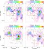 |
Fig. 1 Integrated (220 to 250 km s-1) intensity maps (colors, 20′′ resolution) overlayed with the contours of IRAC 8 μm. The last (eighth) panel shows a three-color image composed of CO(3–2) (blue), [C i] 3P1–3P0 (green), and [C ii] (red). The red lines outline the observed area. Blue asterisks in the CO(3–2) and [C ii] maps mark the positions whose spectra are shown in Fig. 2. Open blue squares and red triangles in the CO(4–3) map show the position of stars with a spectral type of O7 or earlier and O7 to B1, respectively, from Fariña et al. (2009), the filled blue star marks the position of LMC X-1, the blue asterisks are compact H ii regions (Indebetouw et al. 2004), and the red diamond marks the position of an H2O maser (Lazendic et al. 2002). |
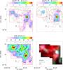 |
Fig. 1 continued. |
In addition to the GREAT [C ii] and [N ii] mapping, we carried out complementary observations with the Atacama Pathfinder Experiment (APEX2; Güsten et al. 2006) of CO(3–2), CO(4–3), 13CO(3–2), and [C i] 3P1–3P0 using the MPIfR heterodyne receiver FLASH+ (Klein et al. 2014), and CO(6–5) and [C i] 3P2–3P1 using the Carbon Heterodyne Array of the MPIfR (CHAMP+; Kasemann et al. 2006) in June, July, September, and November 2012. The backends of FLASH+ are FFTSs with the spectral resolution of 38 kHz and 76 kHz for the 345 GHz and 460 GHz band, respectively. CHAMP+ has two hexagonal arrays each with 7 pixels, simultaneously operated for the 620–720 GHz and the 780–950 GHz frequency range, and the backends are XFFTSs (1.5 GHz bandwidth with 212 kHz resolution). All observations were made in the OTF mode, and the OFF position is the same as in the GREAT observations. Observational parameters are listed in Table 1. Pointing was established on nearby R-Dor with CO lines, repeated every hour, and the pointing uncertainty is less than 2.5′′.
Johansson et al. (1998) mapped 1′ × 1′ around the brightest core of N159 W in CO(3–2) with the Swedish-ESO Submillimetre Telescope (SEST), but it does not cover the whole region of our [C ii] observations. Minamidani et al. (2008) show a larger CO(3–2) map including another prominent core of N159 E obtained with the Atacama Submillimeter Telescope Experiment (ASTE), but these are position switched observations with a grid of 10′′ to 40′′ and are not fully sampled. Therefore, we included CO(3–2) in our APEX observations in order to have sufficient complementary data.
A linear baseline was fitted in the ranges 150–225 km s-1 and 255–350 km s-1 for FLASH+, and 100–220 km s-1 and 255–400 km s-1 for CHAMP+. After discarding spectra with excess noise, the data were spectrally resampled to 1 km s-1 and spatially to 20′′, identical to the resolution of the [C ii] data. As with the GREAT data, reduction up to the spectral resampling was performed using the CLASS software, and the spatial resampling and further analysis was done with IDL.
3. Results and discussion
3.1. Spatial and velocity structures
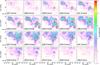 |
Fig. 3 1 km s-1 wide channel maps of the [C ii] emission overlayed with the contours of the CO(3–2) emission. The contours start from 1.5 K with a spacing of 1.5 K. The central velocity is written in each panel. |
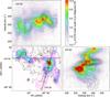 |
Fig. 4 (Lower left) CO(3–2) integrated intensity map overlayed with the contours of IRAC 8 μm (same as Fig. 1), together with two lines marking the two cuts, along which the p − v diagrams are shown in the upper left and lower right panel. (Upper left/lower right) The p − v diagrams of the [C ii] (color) and CO(3–2) (contour) in Tmb [K]. The contour spacing is 1 K. The position axis is horizontal in the upper left panel (cut a)) and vertical in the lower right panel (cut b)), so that the position aligns with the position of the lower left panel. |
Figure 1 shows the integrated intensity maps of CO(3–2), (4–3), (6–5), 13CO(3–2), [C i] 3P1–3P0 and 3P2–3P1, and [C ii], overlayed with the contours of IRAC 8 μm from the Spitzer data archive. We estimate the uncertainty of the integrated intensity (σI [K km s-1]) based on the baseline noise of the spectrum at each position of the resampled map (σrms, Table 1), and the velocity range used for the integrated intensity (220–250 km s-1). In Fig. 1, pixels that have an integrated intensity smaller than 3σI were masked.
As shown in the following, the velocity structure strongly varies across the observed area, and from line to line. Therefore, the integrated intensity map has to be combined with spectral information to interpret the spatial structure. Spectra at selected positions (marked in the CO(3–2) and [C ii] maps of Fig. 1) are shown in Fig. 2; Fig. 3 shows the channel maps of the [C ii] and CO(3–2) emission; and the position-velocity (p − v) diagram of CO(3–2) and [C ii] along two selected cuts are shown in Fig. 4.
In a first step of our analysis we confirmed that our CO(3–2) map reproduces bright cores shown by Johansson et al. (1998) and Minamidani et al. (2008). At N159 W (position 1 in Figs. 1 and 2, p1 in the following), CO(3–2) and all other lines show a wider (~8 km s-1 in FWHM) velocity profile compared to surrounding regions. Regions around p1 (p2, p3, and p4) show narrower profiles with different central velocities, which may blend at p1. The integrated intensity peak of CO(3–2) is shifted southwest compared to the peak in IRAC 8 μm, and the IRAC 8 μm has a cometary shape facing northeast. The spatial distribution indicates a stratification from the northeast as an ionizing front to the molecular cloud toward the southwest. On the other hand, CO(3–2) in the northeast of N159 W does not completely vanish, but shows a weak peak (p3); a very weak east-west bridge along IRAC 8 μm is still seen in CO(3–2) (including p8). The cut (a) in the p − v diagram of CO(3–2) (Fig. 4) goes through p2, p3, p8, and p9, and it shows that the weak bridge connects clumps at p3 and p9 in the velocity as well, indicating that these clumps are not independent but rather connected with each other. The core south of N159 W (p4) is not strong in CO(3–2). From this core, a long ridge continues toward the south up to the edge of the map with a large velocity gradient (cut (b) in Fig. 4 and p15). On the western side, there is another north-south ridge connected to N159 W. It contains a strong core in both CO(3–2) and IRAC 8 μm at the southern edge (p14, the H2O maser source). At N159 E, the CO(3–2) peak (p10) shifts to the east compared to IRAC 8 μm, and the extension to the southeast is also the east side of the IRAC 8 μm ridge. The structure to the southwest from N159 E (p9) fills the gap in IRAC 8 μm, and is connected to the bridge coming from N159 W.
The spatial structure of prominent cores in the integrated intensity maps of CO(3–2), CO(4–3), CO(6–5), and 13CO(3–2) is similar, but the relative strength between cores looks different. For example, the relative strength of p4 to p1 is larger in CO(6–5) than in CO(3–2), indicating a difference in the physical conditions in the different cores. Moreover, the spectral profile of CO(6–5) shows a clear difference with CO(3–2) at some positions because the different velocity components trace different clumps with different physical properties. For example at p7 (Fig. 2), the CO(4–3) and (3–2) emissions have two significant velocity components at ~235 km s-1 and ~240 km s-1, while the CO(6–5) emission at ~235 km s-1 just shows a wing, and its ~240 km s-1 component is very strong in terms of the ratio to CO(4–3) or (3–2). At p6, both the CO(6–5) and [C i] 3P2–3P1 emission have a peak at ~237 km s-1 and especially the CO(6–5) emission is strong, while CO(4–3) and (3–2) have a broad velocity profile peaking at >240 km s-1, and [C i] 3P1–3P0 is even not detected. Position 6 is close to LMC X-1, which is the X-ray binary including a black hole with a mass of ~11 M⊙ (Orosz et al. 2009) and an O7 III companion (Cowley et al. 1995). The ~237 km s-1 component may originate in a clump that is affected by strong X-ray emission from LMC X-1.
The [C i] 3P1–3P0 map and spectra show an overall similarity with CO(3–2), but the two north-south ridges south of N159 W are stronger in [C i] 3P1–3P0. Position 15 is the peak in [C i] 3P1–3P0, whereas the peak there is not clearly seen in other emission lines. The peak of the western ridge shifts slightly to the north in [C i] 3P1–3P0. The [C i] 3P2–3P1 emission is detected in a wide area of N159 W and around the peak of [C i] 3P1–3P0 in N159 E. It is detected in only a small area around N159 E, which may be because of the shorter observing time and thus the lower sensitivity there (Table 1).
The [C ii] emission shows significantly different velocity profiles and integrated intensity maps from the other tracers. It typically has a wider velocity profile, except for a few positions. At p1 and p14, all the lines have a wider and narrower velocity profile than the other positions, respectively, and there is no significant difference in the width between [C ii] and other emissions, except that the peak velocity of the [C ii] emission at p1 is shifted to a smaller velocity (Figs. 2 and 4). At p9–p12, the [C ii] emission is not only wider than in the other tracers, but the peak velocity is also shifted by a few km s-1. The integrated intensity of [C ii] spatially matches the IRAC 8 μm: in N159 W, their peaks match around p1 while those of CO and [C i] emission are shifted southwest, and in N159 E their peaks are instead at p11 in contrast to the CO and [C i] peak at p10. An exception is p13, where the [C ii] emission indicates a clump but there is no corresponding IRAC 8 μm emission. All CO and [C i] emission lines are also very weak, and the Hα map by Chen et al. (2010) and the 843 MHz radio continuum map by Mills & Turtle (1984) show the presence of ionized gas position, so that it is likely that the [C ii] emission at p13 also originates in the ionized gas component. Unfortunately, our [N ii] map, which would allow the [C ii] contribution from ionized gas to be estimated, does not cover this position. The ridge-like structure between N159 W and E (including p8) is significant in [C ii]. The p − v diagram of cut (a) in Fig. 4 shows that the velocity gradient and the central velocity are similar between CO(3–2) and [C ii], indicating that the emission along the cut in the two tracers does not come from fully independent clouds but is related, although the [C ii] emission has a much wider line width. At p7, the velocity component at ~240 km s-1, which is significant in CO(6–5), is not detectable in the [C ii] emission.
We compare our [C ii] observations with previous studies and archival data from Herschel/PACS. Israel et al. (1996) mapped the N159 region with FIFI/KAO; they quote a beam solid angle as a 68′′ disk, which corresponds to a Gaussian FWHM of 64′′. We convolved our map to 64′′ resolution and derive a line integrated intensity of (6.0–6.3) × 10-4 erg cm-2 s-1 sr-1 at the peak in N159 E and W, whereas their result was (3.5–4.0) × 10-4 erg cm-2 s-1 sr-1. Boreiko & Betz (1991) detected the [C ii] emission at N159 FIR(NE) with their far-infrared heterodyne Schottky-mixer receiver on the KAO, showing a peak antenna temperature of 5.3 K and an integrated intensity of 4.8 × 10⁻⁴ erg cm-2 s-1 sr-1 in the 43′′ FWHM beam. Convolving our map to 43′′ and extracting the spectrum at their measured position (which is 25′′ off from our peak of N159 E), we obtain a peak main beam temperature of 5.9 K and an integrated intensity of 5.9 × 10⁻⁴ erg cm-2 s-1 sr-1. The value measured with GREAT is 10–20% higher, but considering that we are comparing the antenna temperature with the main beam temperature for an extended source, the two observations are compatible. We also retrieved [C ii] observations with PACS from the Herschel data archive, and averaged the spectra in a 20′′ diameter circle based on the geometrical overlap of the PACS spaxels. The values derived for N159 W (p1 and p4) and E (p10 and p11) are (6.1, 7.7, 7.4, and 8.2) × 10-4 erg cm-2 s-1 sr-1 for PACS and (7.2, 10.8, 8.4, and 10.3) × 10-4 erg cm-2 s-1 sr-1 for GREAT, showing that the PACS intensity is 0.7–0.9 of the GREAT intensity. We consider this difference to be within the calibration uncertainties of both instruments.
3.2. Quantitative analysis of the velocity profiles
To investigate quantitatively the velocity profiles and their differences in different emission lines, we fit the CO(3–2) spectra with two Gaussians, and apply the fitted center velocity and width in the fit to the other emission lines, fitting only their amplitudes. Across the map, there is no position that has more than two clearly separate velocity components. In order to handle positions where a de-composition into two velocity components is not possible, we first fit the CO(3–2) spectra with two Gaussians with center, width, and amplitude as free parameters, and when the separation of the fitted center of the two Gaussians is less than 1 km s-1, or the fitted amplitude of one of the Gaussians is less than the noise of the baseline, we re-fit the spectra with a single Gaussian. For the positions where the two velocity components are not clearly separated, the fitting may not be unique, but the sum of the integrated intensity of the two components is robust. Once the width(s) and center(s) of the Gaussian(s) from the CO(3–2) fit are determined, we use these values as fixed parameters in the fitting of the other emission lines, thereby leaving their amplitude as the only free parameter. In these fits, we restricted the spectral range to be fitted to half of the FWHM of the CO 3–2 fit, as long as there is a data point in this range (otherwise we expand the fitting range to the FWHM) to make sure that the peak of the line is well fitted when the profile of the line is different from that of CO(3–2). This procedure allows us to identify how well the other emission lines match the velocity structure visible in CO(3–2) and to identify whether the integrated line emission from the other tracers shows evidence for additional velocity components not visible in CO(3–2).
Figure 5 shows the relation between the integrated intensity and the sum of the fitted Gaussians for each emission line. For CO(3–2), both estimates match perfectly, which guarantees that the fitting with two Gaussians is appropriate. For CO(4–3) and CO(6–5), the integrated intensity is also very well reproduced by the sum of the fitted Gaussians, confirming that the three CO emission lines contain the same two velocity components and give no indication of additional ones. On the other hand, the plots for 13CO(3–2) and [C i] 3P1–3P0 show that the sum of the fitted Gaussian provides larger values by 5–10% than the integrated intensity where the emissions are strong. The [C i] 3P2–3P1 emission may have the same trend for the six strongest data points, but the S/N of the line is much smaller and the trend is not conclusive. Looking at individual spectra, we find that this is because the line widths of 13CO(3–2) and [C i] 3P1–3P0 are slightly narrower at these positions than those of CO(3–2). When we fit the spectra with the width as a free parameter, but fixing the center and the amplitude to the values that we get in the previous fit, the integrated intensity is well produced in both lines. This is likely an optical depth effect because the CO(3–2) and CO(4–3) are optically thick at the line center, the optical depth of the CO(6–5) emission at the strongest position is about unity, whereas the 13CO(3–2) and [C i] emissions are optically thin (see Sect. 3.3). In any case, the difference in the line width is small, since the dynamics makes the line width broader than the thermal width.
The largest difference is for the case of [C ii]. The plot for [C ii] in Fig. 5 shows a clear trend: the sum of the fitted CO-constrained Gaussians only contributed a fraction of the total flux calculated by the integration over the whole velocity range. The large scatter in the plot also indicates a large variation in the fraction of the [C ii] flux in the velocity components correlated with the CO and [C i] emission. For example, at the center of N159 W (p1, see Figs. 1 and 2), ~20% of the [C ii] integrated line emission cannot be contributed by CO-constrained Gaussians, whereas this ratio is ~40% at p7 and more than 50% at p9. The origin for this [C ii] emission may be due to gas ablating from the dense cloud cores, or may be due to additional gas not immediately associated with the dense cores.
We also examined the ratio of the integrated intensity of the different emission lines derived as the sum of the fitted Gaussians to that of CO(3–2). They show clear spatial variations, which is already visible from the example spectra (Fig. 2). The [C ii]/CO(3–2) ratio varies most significantly: more than one order of magnitude across the map. The ratio is low where the CO(3–2) emission is strong (0.6–1 for p1, p10, and p14), indicating a low radiation field and/or a high density (Röllig et al. 2006; Kaufman et al. 2006), and it increases towards regions where diffuse gas is likely dominant (~11 at p7). A full analysis of these amplitude ratios using PDR modeling will be presented in the follow-up paper (Okada et al., in prep.).
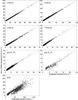 |
Fig. 5 Integrated intensity as a sum of the fitted Gaussians vs. the integration over 220–250 km s-1. The blue line corresponds to both values being equal. |
3.3. Column densities of C+, C, and CO
In this section, we present and discuss the spectral and spatial variations of C+, C, and CO column densities and their ratios. We derive column densities under the simplifying assumption of local thermodynamic equilibrium (LTE) for each species, and a uniform excitation temperature (Tex) for different velocity bins at each position.
Assuming that CO and 13CO have the same Tex and beam (area) filling factor (η), the peak temperature (TB) ratio of CO(3–2) and 13CO(3–2) is described by [1 − exp( − τ12)] / [1 − exp( − τ13)], where τ12 and τ13 are the peak optical depth of the CO(3–2) and 13CO(3–2) emission, respectively. We assume an isotope ratio 12C/13C of 49 as derived for the LMC/N113 region by Wang et al. (2009) and use it as τ12/τ13. We derive τ13 by solving Eq. (1) numerically pixel by pixel,  (1)τ13 varies across the map from 0.06 to 0.5, which corresponds to τ12 = 3–35, i.e., CO(3–2) emission is optically thick everywhere. In general, Tex can be expressed as
 ![Mathematical equation: \begin{equation} T_\mathrm{ex}=\frac{h\nu}{k}\left[\ln\left\{\left(1-{\rm e}^{-\tau}\right)\eta\frac{h\nu}{kT_\mathrm{B}}+1\right\}\right]^{-1}. \label{eq:tex} \end{equation}](/articles/aa/full_html/2015/08/aa25630-15/aa25630-15-eq69.png) (2)Here we use τ13 and TB(13CO(3–2)) to derive Tex of CO. The resulting Tex for the case of η = 0.5 is shown in Fig. 6a. In the figure, the positions of early-type stars (earlier than B4) from Fariña et al. (2009), YSOs from Chen et al. (2010), and OB star candidates from Nakajima et al. (2005) (taken from Chen et al. 2010) are overplotted. Most of the cores are associated with one or more of these, which is consistent with a higher Tex at those positions. The calculation with η = 1 gives a lower limit of Tex, and the Tex at N159 W is 21 K, 36 K, and 150 K for η = 1, 0.5, and 0.1, respectively. Galametz et al. (2013) derive a dust temperature from the far-infrared continuum emission with 36′′ resolution, which is 30–35 K in our observed region. When we estimate Tex at N159 W and E in the same spatial resolution, η = 0.3–0.4 gives the same temperature for Tex as their dust temperature. Minamidani et al. (2011) derive the kinetic temperature from a LVG analysis with 45′′ resolution to be 40–82 K and 65–151 K in N159 W and E, respectively. If we assume that Tex equals their kinetic temperature, it requires a value for η of <0.3. The derived range of filling factors is consistent with the reasonable scenario, that clumps with an enhanced density by more than one or two orders of magnitude fill ~60% or ~35% of the projected area, respectively. In the following, we use the results for η = 0.5, together with η = 0.1 and 0.2 for some cases.
(2)Here we use τ13 and TB(13CO(3–2)) to derive Tex of CO. The resulting Tex for the case of η = 0.5 is shown in Fig. 6a. In the figure, the positions of early-type stars (earlier than B4) from Fariña et al. (2009), YSOs from Chen et al. (2010), and OB star candidates from Nakajima et al. (2005) (taken from Chen et al. 2010) are overplotted. Most of the cores are associated with one or more of these, which is consistent with a higher Tex at those positions. The calculation with η = 1 gives a lower limit of Tex, and the Tex at N159 W is 21 K, 36 K, and 150 K for η = 1, 0.5, and 0.1, respectively. Galametz et al. (2013) derive a dust temperature from the far-infrared continuum emission with 36′′ resolution, which is 30–35 K in our observed region. When we estimate Tex at N159 W and E in the same spatial resolution, η = 0.3–0.4 gives the same temperature for Tex as their dust temperature. Minamidani et al. (2011) derive the kinetic temperature from a LVG analysis with 45′′ resolution to be 40–82 K and 65–151 K in N159 W and E, respectively. If we assume that Tex equals their kinetic temperature, it requires a value for η of <0.3. The derived range of filling factors is consistent with the reasonable scenario, that clumps with an enhanced density by more than one or two orders of magnitude fill ~60% or ~35% of the projected area, respectively. In the following, we use the results for η = 0.5, together with η = 0.1 and 0.2 for some cases.
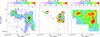 |
Fig. 6 a) CO excitation temperature Tex assuming a beam filling factor η = 0.5 overlayed with contours of CO(3–2) integrated intensity. The positions of YSOs identified by Chen et al. (2010) are marked with asterisks, OB stars (earlier than B4) from Fariña et al. (2009) are marked with triangles, and OB star candidates from Nakajima et al. (2005), taken from Chen et al. (2010), are marked with circles. b) Tex derived from the two [C i] lines overlayed with the contours of [C i] 3P1–3P0 integrated intensity. c) Tex derived by assuming τ = 1 for the [C ii] emission overlayed with the contours of [C ii] integrated intensity. |
The optical depth of an emission line τν is related to the column density of the lower state Nl by ![Mathematical equation: \begin{equation} \tau_\nu=\frac{c^2}{8\pi}\frac{1}{\nu^2_0}\frac{g_u}{g_l}N_lA_{ul}\left[1-\exp\left(-\frac{h\nu_0}{kT_\mathrm{ex}}\right)\right]\phi_\nu\label{eq:tau} , \end{equation}](/articles/aa/full_html/2015/08/aa25630-15/aa25630-15-eq81.png) (3)where subscripts u and l indicate the upper and lower state, g is the statistical weight, Aul is the Einstein coefficient, and φν is the normalized line profile (Wilson et al. 2013). Under the LTE assumption
(3)where subscripts u and l indicate the upper and lower state, g is the statistical weight, Aul is the Einstein coefficient, and φν is the normalized line profile (Wilson et al. 2013). Under the LTE assumption  (4)where Ntot is the total column density, El is the energy of the lower state, and Z is the partition function
  (5)Therefore, the column density in each velocity bin (dNv) can be derived as
 ![Mathematical equation: \begin{equation} {\rm d}N_v=\tau_v\times\frac{8\pi\nu^2_0}{c^2}\frac{Z}{g_u}\frac{1}{A_{ul}}\exp\left(\frac{E_l}{kT_\textrm{ex}}\right)\left[1-\exp\left(-\frac{h\nu_0}{kT_\textrm{ex}}\right)\right]^{-1} {\rm d}v\label{eq:dN_v} , \end{equation}](/articles/aa/full_html/2015/08/aa25630-15/aa25630-15-eq93.png) (6)τv is derived from the brightness temperature at each velocity bin (TB(v)) as
(6)τv is derived from the brightness temperature at each velocity bin (TB(v)) as ![Mathematical equation: \begin{equation} \tau_v=-\ln\left[1-\frac{kT_\mathrm{B}(v)}{\eta h\nu}\left\{\exp\left(\frac{h\nu}{kT_\mathrm{ex}}\right)-1\right\}\right] \label{eq:tau_v} . \end{equation}](/articles/aa/full_html/2015/08/aa25630-15/aa25630-15-eq96.png) (7)In the case of the CO J + 1 → J transition, El = hBJ(J + 1), gu = 2(J + 1) + 1, Z = kTex/hB, and
(7)In the case of the CO J + 1 → J transition, El = hBJ(J + 1), gu = 2(J + 1) + 1, Z = kTex/hB, and  (Wilson et al. 2013), therefore
 ![Mathematical equation: \begin{eqnarray} {\rm d}N_v(\mathrm{CO})&=&\,\tau_v\times\frac{3ckT_\mathrm{ex}}{8\pi^3\nu_0 B\mu^2}\frac{1}{J+1}\exp\left(\frac{hBJ(J+1)}{kT_\mathrm{ex}}\right)\nonumber\\ &&\times\left[1-\exp\left(-\frac{h\nu_0}{kT_\mathrm{ex}}\right)\right]^{-1}{\rm d}v, \end{eqnarray}](/articles/aa/full_html/2015/08/aa25630-15/aa25630-15-eq102.png) (8)where μ is the dipole moment and B is the rotational constant. We used TB(v) of 13CO(3–2) and derived dNv(13CO) and converted it to dNv(CO) by multiplying 12C/13C = 49. The total column density N(CO) was derived by integrating dNv(CO) over the frequency range corresponding on the velocity of 220–250 km s-1 (Fig. 8). The spatial distribution of N(CO) follows the integrated intensity of CO(3–2) and Tex (Fig. 6a).
(8)where μ is the dipole moment and B is the rotational constant. We used TB(v) of 13CO(3–2) and derived dNv(13CO) and converted it to dNv(CO) by multiplying 12C/13C = 49. The total column density N(CO) was derived by integrating dNv(CO) over the frequency range corresponding on the velocity of 220–250 km s-1 (Fig. 8). The spatial distribution of N(CO) follows the integrated intensity of CO(3–2) and Tex (Fig. 6a).
In Fig. 7 we compare the observed peak temperatures TB of CO(4–3) and CO(6–5) with the expected ones from the peak (in terms of velocity) of dNv(CO) assuming that all transitions have the same Tex and η. In the case of η = 0.5, the observed TB is well reproduced, indicating that the assumption of identical Tex and η for all transitions is justified. When η = 0.1, the observed TB of CO(4–3) and CO(6–5) is systematically higher by ~20% and ~60%, respectively. The fact that the observed TB of CO(6–5) is weaker is likely due to CO(6–5) not being thermalized. The critical densities of CO(3–2) and CO(6–5) are (3–4) × 104 cm-3 and 3 × 105 cm-3, respectively, for 10–100 K (calculated using Flower 2001; Goorvitch 1994). Minamidani et al. (2011) derived n(H2) of (4–5) × 103 cm-3 for N159 W and E, and Pineda et al. (2008) discuss the result of PDR modeling with an average density of the clump ensemble of about 105 cm-3. These densities are consistent with the assumption that the CO(6–5) emission does not reach LTE, in contrast to CO(3–2). Calculations with the RADEX radiative transfer program show that the CO(3–2)/CO(6–5) intensity ratio at 30–100 K changes by more than a factor of 2 between 104–105 cm-3 (van der Tak et al. 2007), which can explain the CO(6–5) discrepancy in Fig. 7 in this work. Alternatively, it is also possible that η of CO(6–5) is smaller than that of CO(3–2) because it traces warmer gas which is expected to be in a thinner layer.
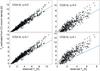 |
Fig. 7 Peak brightness temperature of CO(4–3) (left panels) and CO(6–5) (right panels) estimated from the CO column density derived by using Tex under the assumption of η = 0.5 (upper panels) and 0.1 (lower panels) for all CO lines against observed TB (20′′ resolution). Blue lines indicate the case where the estimated and observed TB is the same. |
At positions where both [C i] lines are detected, we derive the [C i] excitation temperature Tex and the peak optical depth τ from their ratio and their peak temperature. The optical depth ratio of both transitions in [C i] can be expressed in terms of Tex under the LTE assumption (Eq. (3)). Combining with Eq. (2) for both transitions provides two independent equations in terms of Tex, η, and τ10 (the optical depth of 3P1–3P0) as unknown variables, and TB as observed quantities. Since the S/N of [C i]3P2–3P1 is low, and the line profiles of the two [C i] lines are the same with the exception of a few positions mentioned in Sect. 3.1, we did not use directly TB(3P1–3P0) and TB(3P2–3P1) as observed variables, but used TB(3P1–3P0) and I(3P2–3P1)/I(3P1–3P0), where I is the integrated intensity. We calculated τ10 and Tex numerically for individual η. The resultant τ10 is less than 1 at all pixels for all η, and Tex is insensitive to η. For the fully optically thin case, I(3P2–3P1)/I(3P1–3P0) is proportional to τ21/τ10, therefore independent on η. The median of Tex across the map is 70–80 K for η ≥ 0.2 and 90 K for η = 0.1. In Fig. 6b the spatial distribution of Tex for η = 0.5 is shown. In contrast to Tex derived from the CO emissions, Tex for [C i] is lower at the N159 W core than the surroundings. If we assume that Tex of CO and [C i] are similar (within 10 K), the comparison at p1 (N159 W), p4, and p10 (N159 E) gives η of 0.3–0.4, <0.2, and 0.1–0.2, respectively.
To derive the total neutral atomic carbon column density from Eqs. (6) and (7), we sum over the three fine structure levels 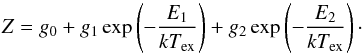 (9)Since the region where the [C i] 3P2–3P1 emission is detected is small and the uncertainty of the derived temperature is relatively large because of the weak [C i] 3P2–3P1 emission, we examine both cases using the Tex derived from the [C i] ratio and a constant value of its median to estimate the column density. The derived column densities match within 10%, even less than 5% at most positions. In the following, we use the case with constant Tex (Fig. 8) because it covers a larger spatial area.
Since there is only a single [C ii] line, we need to assume its optical depth in order to estimate Tex using Eq. (2), or assume a constant Tex for the column density derivation. In several Galactic PDRs, the optical depth of the [C ii] line is estimated to be (0.6–3.2) using the hyperfine components of the [13C ii] emission (Ossenkopf et al. 2013; Graf et al. 2012; Stacey et al. 1991). In the N159 region, the strongest [13C ii] hyperfine component is blended with the broad main isotope line, and the upper limit of the second strongest [13C ii] hyperfine component does not give a useful constraint to the optical depth of [C ii]. Figure 6c shows the estimate of Tex for a constant optical depth τ = 1 (see Kaufman et al. 1999) for the peak velocity and η = 0.5. The spatial distribution follows the distribution of the [C ii] brightness because a stronger peak temperature is attributed to a higher temperature. When we assume τ = 0.5, Tex increases by 15–37%. For the optically thin case, τ is coupled with η. When we assume τ = 3 and τ ≫ 1, Tex goes down typically by 10–16% and 11–18%, respectively. The latter case gives the lower limit of Tex.
The column density of C+ is derived using Eqs. (6) and (7), together with the first two terms in Eq. (9) because C+ is a two-level system. We examine both cases using the Tex derived by assuming τ = 1 and a constant value (Figs. 8c and d). The constant value is determined, depending on η, as the largest value of Tex estimated from the τ ≫ 1 case across the map, which is 67 K and 199 K for η = 0.5 and 0.1, respectively. In this way, the constant Tex is above the Tex lower limit at any position of the map. We then estimate τ in case of this constant Tex. It is fully optically thick at the C+ peak of p4, and regions around other peaks (N159 W, E, p7) have τ ~ 1 at the peak velocity. For the constant Tex case, the contrast of the [C ii] emission is attributed to the difference in τ; therefore, the derived column density basically reproduces the [C ii] intensity distribution (Fig. 8d). For the constant τ case, the stronger [C ii] emission is attributed to a higher Tex (Fig. 6c), but the column density is insensitive to Tex. Thus, the large variation of the [C ii] velocity profile causes a different τν profile from position to position and results in a different spatial distribution of N(C+) from the Tex and the integrated intensity distribution. The higher N(C+) in the eastern part of the map (Fig. 8c) is due to a wider line profile there because the constant τ is at the peak of the line and a wider line makes the integrated column density larger. Qualitatively, positions with strong [C ii] emission are the outer part of PDRs where the temperature is higher and the column density of C+ is higher than toward the molecular core. Therefore, the assumptions of constant τ and constant Tex are the two extreme cases, and the reality should be somewhere in between. In the following analysis we use the constant Tex case because it is unlikely that the optical depth is the same between cores or the [C ii] peak positions and regions in between where the [C ii] emission is much fainter.
 |
Fig. 8 Total column density of CO, C, and C+ for the η = 0.5 case overlayed with the contours of the integrated intensity of CO(3–2) in a), [C i] 3P1–3P0 in b), and [C ii] in c) and d). N(C) is derived by assuming Tex= 74 K, and for N(C+), both cases of τ = 1c) and Tex= 67 K d) are shown (see text). |
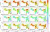 |
Fig. 9 Channel map of the fraction of C+ column density against the total carbon column density (dNv(C+)/ (dNv(C+)+ dNv(C)+ dNv(CO))) using the C+ column density derived from Tex= 67 K and assuming η = 0.5. The velocity bin is 1 km s-1, and the central velocity is shown in each panel. |
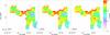 |
Fig. 10 Fraction of total column density of C+, i.e., N(C+)/(N(C+)+ N(C)+ N(CO)), for different η. |
Assuming that N(C+)+ N(C)+ N(CO) is the total column density of the carbon species in the gas phase, we estimate NH using a carbon abundance of 7.9 × 10⁻⁵ (Garnett 1999) for selected positions and η (Table 2). For a hydrogen density of 104–105 cm-3 (see above), the depth of the cloud is 0.3–3 pc for 1023 cm-2. The typical projected size of clumps in the observed region is 30′′, which corresponds to 7 pc at a distance of 50 kpc. Assuming that the projected size is on the same order as the depth of clouds, a smaller η would be preferred. The total mass, obtained by integrating over the whole observed area, is 2.2 × 10⁵M⊙, 4.4 × 10⁵M⊙, and 8.5 × 10⁵M⊙ for η = 0.5, 0.2, and 0.1, respectively.
Total column density of C+, C, and CO, and NH estimated from N(C+)+ N(C)+ N(CO).
With dNv of each species, we estimate the fraction of each species in each velocity bin. Figure 9 shows the channel map of the C+ column density fraction against the total column density of the three species, i.e., dNv(C+)/(dNv(C+)+ dNv(C)+ dNv(CO)), in the case of η = 0.5 and the C+ column density derived from the constant Tex of 67 K. There are two prominent features here. One is given by dips in the C+ column density fraction at the N159 W core (~240 km s-1), N159 E (~233 km s-1), and southwest of N159 E (~235 km s-1). The C+ fraction drops to 30%, 50%, and 40%, respectively, and the rest is shared by [C i] (30%, 20%, 20%) and CO (40%, 30%, 40%). On the other hand, C+ is dominant at all velocity bins in the region between N159 W and E. The second feature is that C+ is clearly dominant at almost all positions in the map for velocities far from the line center (≲230 km s-1 and ≳240 km s-1). The total column density depends on the assumed η, but the fraction of the column density of each species is less sensitive to η, and this spatial and spectral trend is largely independent of the value assumed for η. Figure 10 shows the fraction of the total C+ against total carbon column density, namely N(C+)/(N(C+)+ N(C)+ N(CO)) for different values of η, confirming the spatial trend, and Fig. 11 shows the spectra of the column density fraction averaged over the map, which clearly demonstrates that C+ is the dominant species at velocities of below 230 km s-1 and above 240 km s-1.
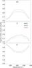 |
Fig. 11 Spectra of the fraction of CO, C, and C+ column density against the total column density, i.e., dNv(C+) or dNv(C) or dNv(CO) over (dNv(C+)+ dNv(C)+ dNv(CO)) averaged over the map. |
3.4. Estimate of the [C II] emission coming from ionized gas
We examine the ionized gas contribution to the [C ii] emission using the [N ii] 205 μm emission. Since the [N ii] emission is very weak, we convolve the [N ii] emission to a spatial resolution of 50′′ and a spectral resolution of 2 km s-1. The integrated intensity map (Fig. 12) shows an anti-correlation between the [C ii] and [N ii] emission, which indicates that most of the emission does not come from the ionized gas, which also emits in [N ii]. To estimate the contribution of the ionized gas to the [C ii] emission quantitatively, we compare the observed [N ii]/[C ii] ratio with predictions based on a simple isothermal three-level system, for electron temperatures in the range 7000–12 000 K. In Table 3, the observed ratios (in 50′′ beams) are listed for the four positions indicated in Fig. 12, as well as the average over the blue box area in Fig. 12 and the average over the whole observed area. For the calculations we used the elemental abundances of C and N for LMC H ii regions as given by Garnett (1999). The N abundance is consistent with Vermeij & van der Hulst (2002). We assume optically thin emission and LTE conditions (high density limit). These assumptions provide an upper limit on the contribution of the ionized gas to the [C ii] emission for the following reasons. When we calculate [N ii] 205 μm/[C ii] 158 μm as a function of the electron density, it has a maximum around 50–100 cm-3 and reaches its minimum (0.074) in the high density limit. The [N ii] 205 μm/[C ii] 158 μm ratio is much less sensitive to the electron density than [N ii] 122 μm/[C ii] 158 μm; the former varies by only ~65% over the whole electron density range, whereas the latter varies by one order of magnitude. Still, if the electron density is at a range where the predicted [N ii] 205 μm/[C ii] 158 μm ratio is higher than 0.074, the [C ii] intensity attributed to the ionized gas becomes lower. If the observed [C ii] emission is optically thick (or τ ~ 1, see previous section), the optical-depth-corrected [C ii] emission would be stronger, so the fraction of the ionized gas contribution would decrease. The maximum possible contribution from the ionized gas to the [C ii] emission is 40–60% at positions A, B, and D, where the [N ii] emission has a peak, with only 20% at position C. Position C is the [C ii] peak, which has only very weak corresponding CO and [C i] emission (see p7 in Sect. 3.1). Using the [N ii] emission, we exclude the ionized gas as a dominant origin of the [C ii] emission at this position. The average contribution over the blue box in Fig. 12, where the [N ii] is detected (at 50′′ resolution), is 30%, and over the whole observed area it is 15% (Table 3).
In Fig. 13 the velocity profiles of [C ii] and [N ii] at these four positions are compared. We fit the [N ii] line with a single Gaussian, and the fitted central velocity is indicated as a vertical line. For positions A and B, the difference of the velocity profile between the [N ii] and [C ii] is within the noise, but for positions C and D, [N ii] has a higher central velocity, and the [C ii] profile of the higher velocity wing matches the [N ii] profile, indicating that this velocity component might be associated with the ionized gas. The ratio of [N ii]/[C ii] in the high-velocity wing (>245 km s-1) for position C and D is consistent with their origin in the ionized gas.
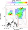 |
Fig. 12 Integrated (220–250 km s-1) intensity map of [N ii] (colors), convolved to 50′′ angular resolution, overlayed with the contours of [C ii] at 20′′ resolution. Blue asterisks show the positions where spectra have been extracted for Fig. 13. The inserted spectrum shows the [N ii] emission averaged in the area marked by the blue box (x-axis is Velocity [km s-1] and y-axis is Tmb [K]). |
The C+ column density in the ionized gas can be directly estimated by the H+ column density (N(H+)) derived from the radio continuum observations.
Maximum possible contribution of the ionized gas to the [C ii] emission based on the integrated intensity ratio of [N ii]/[C ii].
Martín-Hernández et al. (2005) derived the emission measure and the electron density at three compact peak positions by the 6 cm continuum observations using the ATCA. These are the compact H ii regions identified by Indebetouw et al. (2004) and match the [C ii] peaks (blue asterisks in the CO(4–3) panel of Fig. 1; p4, p11, and northeast of p1). The electron density (ne) at these positions is (2.2–3.0) × 103 cm-3, and together with the emission measure it gives N(H+) of (3–9) × 1021 cm-2, and thus N(C+) of (3–7) × 1017 cm-2 if we assume that all carbon atoms are singly ionized. Since two of them are spatially resolved by ATCA having the source size of 4–5′′ and the other one is smaller than the beam size (<2′′), the dilution factor in our 20′′ map is 16–103, which makes the estimate of N(C+) = 4 × 1016 cm-2 for p11 and northeast of p1, and 3 × 1015 cm-2 for p4. They are 2% or less compared to the N(C+) derived from the [C ii] emission (Table 2). However, this should be interpreted as a contribution from the dense ionized gas traced preferably by the radio continuum (its intensity is proportional to  ), but not from the diffuse ionized gas. The Hα map by the Magellanic Cloud Emission-Line Survey (MCELS) shows a different morphology including more extended structure and additional peak positions (Chen et al. 2010). Our [N ii] map does not have a peak at these compact H ii regions, but correlates with Hα, confirming that they instead trace more diffuse ionized gas than the radio continuum because the critical density of the [N ii] 205 μm is 180 cm-3 (Shibai 1992). Since the critical density of the [C ii] 158 μm with the collision partner of electron is 40 (Shibai 1992), it also traces more diffuse ionized gas rather than dense ionized gas. Thus, the [N ii] 205 μm emission is useful for estimating the ionized gas contribution to the [C ii] emission, tracing the same gas. The reason that the [C ii] emission has peaks at the positions of compact H ii regions should be interpreted as a dominant contribution of the PDR gas that surrounds these dense H ii regions and is illuminated by strong the UV radiation.
Theoretical models of H ii region/PDR complexes of solar metallicity gas predict contributions from the ionized gas to the [C ii] emission as high as 40% (Abel et al. 2005) or less than 10% (Kaufman et al. 2006) for most of the physical parameter range. Observations toward Galactic PDRs have in fact provided comparable results. Towards the Carina nebula, Oberst et al. (2011) derive 37% from the [N ii] 205 μm/[C ii] 158 μm ratio, while using the correlation of [C ii] 158 μm with [N ii] 122 μm and [O i] 63 μm Mizutani et al. (2004) find 20%. Giannini et al. (2000) show a 10–30% contribution from the ionized gas in NGC 2024 by CLOUDY modeling. In S171 and σ Sco region, the PDR contribution to the [C ii] emission is estimated by the PDR modeling, and the ionized gas contribution shows a spatial distribution with about 80% at positions closer to the exciting stars, but only 20% or 30% at positions farther away (Okada et al. 2006, 2003). Similarly 10–30% contribution of the ionized gas is reported in several star-forming regions in nearby galaxies with almost solar metallicity (Contursi et al. 2013; Kramer et al. 2005). Lebouteiller et al. (2012) present that 95% of the [C ii] emission arises in PDRs in LMC-N11B, except toward the star cluster for which as much as 15% could arise in the ionized gas. In M33 star-forming regions a typical ionized gas contribution is estimated to be 5–50% (Higdon et al. 2003). In principle in a lower metallicity environment, the [C ii] emission from the H ii region decreases because the size of the H ii region is independent of the metallicity and the metal emission line is proportional to the abundance, while the column of C+ layer in a PDR stays constant. Therefore, the ionized gas contribution in a lower metallicity environment should be lower (Israel & Maloney 2011; Kaufman et al. 2006). However, because of the uncertainties of the results cited above, this dependency has not been demonstrated by observations.
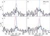 |
Fig. 13 [C ii] (purple) and [N ii] (black; scaled by 10) spectra at positions indicated in Fig. 12 with 2 km s-1 spectral resolution. Blue lines show the result of a single Gaussian fit to the [N ii] emission, and its center is indicated as a vertical line. |
3.5. Spatially resolved I[CII]/IFIR,th
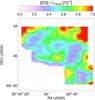 |
Fig. 14 [C ii]/IFIR,th map (see text for the definition) overlayed with the contours of the [C ii] integrated intensity. |
The ratio [C ii]/IFIR has been widely used as a tracer of the photoelectric heating efficiency, under the assumption that [C ii] 158 μm is the dominant cooling line. Here we derive the spatial distribution of this ratio. We obtained the archival data of MIPS 24 μm (the legacy survey of SAGE), PACS 100 μm and 160 μm, and SPIRE 250 μm (the open key time program HERITAGE); applied the color correction; convolved them to a spatial resolution of 20′′; fitted them with a modified blackbody with a single temperature and a spectral index of β = 1.5; and integrated the fitted curve over the total range of the thermal emission. Traditionally, IFIR is defined as the 42–122 μm flux and ITIR is defined as the 3–1100 μm flux (Dale & Helou 2002). Here we use the direct integration of the fitted total thermal emission, and express it as IFIR,th. We do not calculate ITIR because we do not have a spectrum of polycyclic aromatic hydrocarbons (PAHs) at each position, and its contribution to total infrared flux (TIR) can vary in spatially resolved regions. We do not adopt IFIR either because there is no reason to cut the integration at 122 μm. Figure 14 shows the spatial distribution of I[CII]/IFIR,th. The ratio is significantly lower at the N159 W and E cores, being 0.3–0.4%. At the [C ii] peak between N159 W and E (p7), I[CII]/IFIR,th = 0.7–0.8%. These values are in the same range as the results in the LMC/N11 region by Lebouteiller et al. (2012) when considering that TIR, which includes mid-infrared emissions, is 10–35% higher than the total thermal emission (estimate among the sample of PDRs in Okada et al. 2013,except for Ced 201, which is excited by a much later star of B9.5). Israel et al. (1996) present a value of I[CII]/IFIR of 1–2% for the N159 E and W cores. Their much larger value is due to the definition of IFIR and the lower spatial resolution (the FIR emission has a sharper peak at the cores than [C ii]).
There are three possible causes of the lower I[CII]/IFIR,th at the cores. The first possibility is a contribution of the [O i] 63 μm to the cooling. Here we do not directly use the archival PACS spectroscopic data because they do not cover our whole observed region, but the comparison of the [O i] 63 μm and [C ii] 158 μm emissions within their observed area indicates that the intensity of [O i] 63 μm is 30–100% of the [C ii] 158 μm intensity. We plan to observe velocity resolved [O i] 63 μm with GREAT at our next southern flight opportunity and carefully compare the line profile. The second possibility is that the photoelectric heating efficiency is actually low at these cores. The photoelectric heating efficiency is a function of the charging parameter γ = G0T1/2/ne, where G0 is UV radiation field, T is the gas temperature, and ne is the electron density (Bakes & Tielens 1994). When γ is high, dust grains are positively charged. Thus, the photoelectric heating efficiency becomes lower because a higher energy is needed to further ionize them. If there is a strong UV source in the core, γ in the core is high and the heating efficiency could be lower than outside. This may be likely because both N159 E and W possess compact H ii regions (Fig. 1 CO(4–3) panel). Correlation with the fraction of positively ionized PAHs would give more detailed examination of this possibility (Okada et al. 2013), but there are only sparse Spitzer/IRS observations in this region. The third possibility is that later-type heating sources contribute to IFIR,th but not to the photoelectric heating because of the lack of photons with the energy of >6 eV.
4. Summary
We mapped a 4′ × (3′–4′) region in the N159 star-forming region in the LMC in the [C ii] 158 μm and [N ii] 205 μm lines with the GREAT instrument on board SOFIA, as well as CO(3–2), (4–3), (6–5), 13CO(3–2), and [C i] 3P1–3P0 and 3P2–3P1 with APEX, and study their velocity profiles in detail. The variation of the velocity structure over the observed area is large, and the [C ii] emission shows a significantly different velocity profile from the other lines at most positions. Quantitatively, we estimate the fraction of the [C ii] emission that cannot be attributed to the material traced by the CO line profiles to be 20% around the CO cores and up to 50% in the area between the cores. We derived the column density of C+, C, and CO in each velocity bin, and find that the relative contribution from C+ dominates at the velocity range far from the line center, and the area between the CO cores. The origin for this [C ii] emission, at velocities substantially off the velocities of the dense molecular cores traced by CO and [C i], may be due to gas ablating from the dense cloud cores or to additional gas not immediately associated with the dense cores.
To estimate the contribution of the ionized gas to the [C ii] emission, we use the ratio with the [N ii] 205 μm line and show that the ionized gas can contribute up to 19% to the [C ii] emission at its peak position, less than 30% in the area where [N ii] is detected, and less than 15% if averaged over the whole area observed. By comparing the peak velocity of the [C ii] and [N ii] emissions, we provide evidence that a high-velocity wing in the [C ii] emission is likely due to ionized gas. Our study emphasizes that it is essential to resolve the velocity profile in order to distinguish between different cloud components and correctly derive the physical properties of individual components.
GREAT is a development by the MPI für Radioastronomie and the KOSMA/Universität zu Köln, in cooperation with the MPI für Sonnensystemforschung and the DLR Institut für Planetenforschung.
APEX is a collaboration between the Max-Planck-Institut fur Radioastronomie, the European Southern Observatory, and the Onsala Space Observatory.
Acknowledgments
This work is based in part on observations made with the NASA/DLR Stratospheric Observatory for Infrared Astronomy (SOFIA). SOFIA is jointly operated by the Universities Space Research Association, Inc. (USRA), under NASA contract NAS2-97001, and the Deutsches SOFIA Institut (DSI) under DLR contract 50 OK 0901 to the University of Stuttgart. This work is carried out within the Collaborative Research Centre 956, sub-project A3, funded by the Deutsche Forschungsgemeinschaft (DFG). We thank F. Israel for contributing to the FIFI-GREAT comparison. We thank C.-H.R. Chen for providing a list of the OB star candidates.
References
- Abel, N. P., Ferland, G. J., Shaw, G., & van Hoof, P. A. M. 2005, ApJS, 161, 65 [NASA ADS] [CrossRef] [Google Scholar]
- Bakes, E. L. O., & Tielens, A. G. G. M. 1994, ApJ, 427, 822 [NASA ADS] [CrossRef] [Google Scholar]
- Bolatto, A. D., Jackson, J. M., & Ingalls, J. G. 1999, ApJ, 513, 275 [NASA ADS] [CrossRef] [Google Scholar]
- Bolatto, A. D., Jackson, J. M., Israel, F. P., Zhang, X., & Kim, S. 2000, ApJ, 545, 234 [NASA ADS] [CrossRef] [Google Scholar]
- Boreiko, R. T., & Betz, A. L. 1991, ApJ, 380, L27 [NASA ADS] [CrossRef] [Google Scholar]
- Carlhoff, P. 2013, Ph.D. Thesis, Universität zu Köln [Google Scholar]
- Carrera, R., Gallart, C., Hardy, E., Aparicio, A., & Zinn, R. 2008, AJ, 135, 836 [NASA ADS] [CrossRef] [Google Scholar]
- Chen, C.-H. R., Indebetouw, R., Chu, Y.-H., et al. 2010, ApJ, 721, 1206 [NASA ADS] [CrossRef] [Google Scholar]
- Cohen, R. S., Dame, T. M., Garay, G., et al. 1988, ApJ, 331, L95 [NASA ADS] [CrossRef] [Google Scholar]
- Contursi, A., Poglitsch, A., Grácia Carpio, J., et al. 2013, A&A, 549, A118 [NASA ADS] [CrossRef] [EDP Sciences] [Google Scholar]
- Cowley, A. P., Schmidtke, P. C., Anderson, A. L., & McGrath, T. K. 1995, PASP, 107, 145 [NASA ADS] [CrossRef] [Google Scholar]
- Dale, D. A., & Helou, G. 2002, ApJ, 576, 159 [NASA ADS] [CrossRef] [Google Scholar]
- Dedes, C., Röllig, M., Mookerjea, B., et al. 2010, A&A, 521, L24 [NASA ADS] [CrossRef] [EDP Sciences] [Google Scholar]
- De Looze, I., Baes, M., Bendo, G. J., Cortese, L., & Fritz, J. 2011, MNRAS, 416, 2712 [Google Scholar]
- Fariña, C., Bosch, G. L., Morrell, N. I., Barbá, R. H., & Walborn, N. R. 2009, AJ, 138, 510 [NASA ADS] [CrossRef] [Google Scholar]
- Flower, D. R. 2001, MNRAS, 328, 147 [Google Scholar]
- Galametz, M., Hony, S., Galliano, F., et al. 2013, MNRAS, 431, 1596 [NASA ADS] [CrossRef] [Google Scholar]
- Garnett, D. R. 1999, in New Views of the Magellanic Clouds, eds. Y.-H. Chu, N. Suntzeff, J. Hesser, & D. Bohlender, IAU Symp., 190, 266 [Google Scholar]
- Giannini, T., Nisini, B., Lorenzetti, D., et al. 2000, A&A, 358, 310 [NASA ADS] [Google Scholar]
- Goorvitch, D. 1994, ApJS, 95, 535 [NASA ADS] [CrossRef] [Google Scholar]
- Graf, U. U., Simon, R., Stutzki, J., et al. 2012, A&A, 542, L16 [NASA ADS] [CrossRef] [EDP Sciences] [Google Scholar]
- Guan, X., Stutzki, J., Graf, U. U., et al. 2012, A&A, 542, L4 [NASA ADS] [CrossRef] [EDP Sciences] [Google Scholar]
- Güsten, R., Nyman, L. Å., Schilke, P., et al. 2006, A&A, 454, L13 [NASA ADS] [CrossRef] [EDP Sciences] [Google Scholar]
- Heyminck, S., Graf, U. U., Güsten, R., et al. 2012, A&A, 542, L1 [NASA ADS] [CrossRef] [EDP Sciences] [Google Scholar]
- Higdon, S. J. U., Higdon, J. L., van der Hulst, J. M., & Stacey, G. J. 2003, ApJ, 592, 161 [NASA ADS] [CrossRef] [Google Scholar]
- Indebetouw, R., Johnson, K. E., & Conti, P. 2004, AJ, 128, 2206 [NASA ADS] [CrossRef] [Google Scholar]
- Israel, F. P., & Maloney, P. R. 2011, A&A, 531, A19 [NASA ADS] [CrossRef] [EDP Sciences] [Google Scholar]
- Israel, F. P., Maloney, P. R., Geis, N., et al. 1996, ApJ, 465, 738 [NASA ADS] [CrossRef] [Google Scholar]
- Johansson, L. E. B., Greve, A., Booth, R. S., et al. 1998, A&A, 331, 857 [NASA ADS] [Google Scholar]
- Kasemann, C., Güsten, R., Heyminck, S., et al. 2006, in SPIE Conf. Ser., 6275 [Google Scholar]
- Kaufman, M. J., Wolfire, M. G., Hollenbach, D. J., & Luhman, M. L. 1999, ApJ, 527, 795 [NASA ADS] [CrossRef] [Google Scholar]
- Kaufman, M. J., Wolfire, M. G., & Hollenbach, D. J. 2006, ApJ, 644, 283 [NASA ADS] [CrossRef] [Google Scholar]
- Klein, T., Ciechanowicz, M., Leinz, C., et al. 2014, IEEE Transactions on Terahertz Science and Technology, 4, 588 [NASA ADS] [CrossRef] [Google Scholar]
- Kramer, C., Mookerjea, B., Bayet, E., et al. 2005, A&A, 441, 961 [NASA ADS] [CrossRef] [EDP Sciences] [Google Scholar]
- Lazendic, J. S., Whiteoak, J. B., Klamer, I., Harbison, P. D., & Kuiper, T. B. H. 2002, MNRAS, 331, 969 [NASA ADS] [CrossRef] [Google Scholar]
- Lebouteiller, V., Cormier, D., Madden, S. C., et al. 2012, A&A, 548, A91 [NASA ADS] [CrossRef] [EDP Sciences] [Google Scholar]
- Madden, S. C., Poglitsch, A., Geis, N., Stacey, G. J., & Townes, C. H. 1997, ApJ, 483, 200 [NASA ADS] [CrossRef] [MathSciNet] [Google Scholar]
- Madden, S. C., Galametz, M., Cormier, D., et al. 2011, in EAS PS 52, eds. M. Röllig, R. Simon, V. Ossenkopf, & J. Stutzki, 95 [Google Scholar]
- Martín-Hernández, N. L., Vermeij, R., & van der Hulst, J. M. 2005, A&A, 433, 205 [NASA ADS] [CrossRef] [EDP Sciences] [Google Scholar]
- Mills, B. Y., & Turtle, A. J. 1984, in Structure and Evolution of the Magellanic Clouds, eds. S. van den Bergh, & K. S. D. de Boer, IAU Symp., 108, 283 [Google Scholar]
- Minamidani, T., Mizuno, N., Mizuno, Y., et al. 2008, ApJS, 175, 485 [NASA ADS] [CrossRef] [Google Scholar]
- Minamidani, T., Tanaka, T., Mizuno, Y., et al. 2011, AJ, 141, 73 [NASA ADS] [CrossRef] [Google Scholar]
- Mizuno, N., Yamaguchi, R., Mizuno, A., et al. 2001, PASJ, 53, 971 [NASA ADS] [Google Scholar]
- Mizuno, Y., Kawamura, A., Onishi, T., et al. 2010, PASJ, 62, 51 [NASA ADS] [Google Scholar]
- Mizutani, M., Onaka, T., & Shibai, H. 2004, A&A, 423, 579 [NASA ADS] [CrossRef] [EDP Sciences] [Google Scholar]
- Mochizuki, K., Nakagawa, T., Doi, Y., et al. 1994, ApJ, 430, L37 [NASA ADS] [CrossRef] [Google Scholar]
- Mookerjea, B., Ossenkopf, V., Ricken, O., et al. 2012, A&A, 542, L17 [NASA ADS] [CrossRef] [EDP Sciences] [Google Scholar]
- Nakajima, Y., Kato, D., Nagata, T., et al. 2005, AJ, 129, 776 [NASA ADS] [CrossRef] [Google Scholar]
- Oberst, T. E., Parshley, S. C., Nikola, T., et al. 2011, ApJ, 739, 100 [NASA ADS] [CrossRef] [Google Scholar]
- Okada, Y., Onaka, T., Shibai, H., & Doi, Y. 2003, A&A, 412, 199 [NASA ADS] [CrossRef] [EDP Sciences] [Google Scholar]
- Okada, Y., Onaka, T., Nakagawa, T., et al. 2006, ApJ, 640, 383 [NASA ADS] [CrossRef] [Google Scholar]
- Okada, Y., Güsten, R., Requena-Torres, M. A., et al. 2012, A&A, 542, L10 [NASA ADS] [CrossRef] [EDP Sciences] [Google Scholar]
- Okada, Y., Pilleri, P., Berné, O., et al. 2013, A&A, 553, A2 [NASA ADS] [CrossRef] [EDP Sciences] [Google Scholar]
- Orosz, J. A., Steeghs, D., McClintock, J. E., et al. 2009, ApJ, 697, 573 [NASA ADS] [CrossRef] [Google Scholar]
- Ossenkopf, V., Röllig, M., Neufeld, D. A., et al. 2013, A&A, 550, A57 [NASA ADS] [CrossRef] [EDP Sciences] [Google Scholar]
- Pérez-Beaupuits, J. P., Wiesemeyer, H., Ossenkopf, V., et al. 2012, A&A, 542, L13 [NASA ADS] [CrossRef] [EDP Sciences] [Google Scholar]
- Pety, J. 2005, in SF2A-2005: Semaine de l’Astrophysique Francaise, eds. F. Casoli, T. Contini, J. M. Hameury, & L. Pagani, 721 [Google Scholar]
- Pilleri, P., Fuente, A., Cernicharo, J., et al. 2012, A&A, 544, A110 [NASA ADS] [CrossRef] [EDP Sciences] [Google Scholar]
- Pineda, J. L., Mizuno, N., Stutzki, J., et al. 2008, A&A, 482, 197 [NASA ADS] [CrossRef] [EDP Sciences] [Google Scholar]
- Poglitsch, A., Krabbe, A., Madden, S. C., et al. 1995, ApJ, 454, 293 [NASA ADS] [CrossRef] [Google Scholar]
- Röllig, M., Ossenkopf, V., Jeyakumar, S., Stutzki, J., & Sternberg, A. 2006, A&A, 451, 917 [NASA ADS] [CrossRef] [EDP Sciences] [Google Scholar]
- Schneider, N., Güsten, R., Tremblin, P., et al. 2012, A&A, 542, L18 [Google Scholar]
- Shibai, H. 1992, Observational study of large-scale forbidden CII emission by Balloon-Borne Infrared Telescope (BIRT), Tech. Rep. 650 [Google Scholar]
- Simon, R., Schneider, N., Stutzki, J., et al. 2012, A&A, 542, L12 [NASA ADS] [CrossRef] [EDP Sciences] [Google Scholar]
- Stacey, G. J., Townes, C. H., Geis, N., et al. 1991, ApJ, 382, 423 [NASA ADS] [CrossRef] [Google Scholar]
- Sternberg, A., & Dalgarno, A. 1995, ApJS, 99, 565 [NASA ADS] [CrossRef] [Google Scholar]
- Tielens, A. G. G. M., & Hollenbach, D. 1985, ApJ, 291, 722 [NASA ADS] [CrossRef] [Google Scholar]
- van der Tak, F. F. S., Black, J. H., Schöier, F. L., Jansen, D. J., & van Dishoeck, E. F. 2007, A&A, 468, 627 [NASA ADS] [CrossRef] [EDP Sciences] [Google Scholar]
- Vermeij, R., & van der Hulst, J. M. 2002, A&A, 391, 1081 [NASA ADS] [CrossRef] [EDP Sciences] [Google Scholar]
- Wang, M., Chin, Y.-N., Henkel, C., Whiteoak, J. B., & Cunningham, M. 2009, ApJ, 690, 580 [NASA ADS] [CrossRef] [Google Scholar]
- Wilson, T. L., Rohlfs, K., & Hüttemeister, S. 2013, Tools of Radio Astronomy 5th edn. (Springer), 404 [Google Scholar]
- Young, E. T., Becklin, E. E., Marcum, P. M., et al. 2012, ApJ, 749, L17 [NASA ADS] [CrossRef] [Google Scholar]
All Tables
Maximum possible contribution of the ionized gas to the [C ii] emission based on the integrated intensity ratio of [N ii]/[C ii].
All Figures
|
Fig. 1 Integrated (220 to 250 km s-1) intensity maps (colors, 20′′ resolution) overlayed with the contours of IRAC 8 μm. The last (eighth) panel shows a three-color image composed of CO(3–2) (blue), [C i] 3P1–3P0 (green), and [C ii] (red). The red lines outline the observed area. Blue asterisks in the CO(3–2) and [C ii] maps mark the positions whose spectra are shown in Fig. 2. Open blue squares and red triangles in the CO(4–3) map show the position of stars with a spectral type of O7 or earlier and O7 to B1, respectively, from Fariña et al. (2009), the filled blue star marks the position of LMC X-1, the blue asterisks are compact H ii regions (Indebetouw et al. 2004), and the red diamond marks the position of an H2O maser (Lazendic et al. 2002). |
| In the text | |
|
Fig. 1 continued. |
| In the text | |
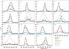 |
Fig. 2 Spectra at selected positions marked in the CO(3–2) panel in Fig. 1. |
| In the text | |
|
Fig. 3 1 km s-1 wide channel maps of the [C ii] emission overlayed with the contours of the CO(3–2) emission. The contours start from 1.5 K with a spacing of 1.5 K. The central velocity is written in each panel. |
| In the text | |
|
Fig. 4 (Lower left) CO(3–2) integrated intensity map overlayed with the contours of IRAC 8 μm (same as Fig. 1), together with two lines marking the two cuts, along which the p − v diagrams are shown in the upper left and lower right panel. (Upper left/lower right) The p − v diagrams of the [C ii] (color) and CO(3–2) (contour) in Tmb [K]. The contour spacing is 1 K. The position axis is horizontal in the upper left panel (cut a)) and vertical in the lower right panel (cut b)), so that the position aligns with the position of the lower left panel. |
| In the text | |
|
Fig. 5 Integrated intensity as a sum of the fitted Gaussians vs. the integration over 220–250 km s-1. The blue line corresponds to both values being equal. |
| In the text | |
|
Fig. 6 a) CO excitation temperature Tex assuming a beam filling factor η = 0.5 overlayed with contours of CO(3–2) integrated intensity. The positions of YSOs identified by Chen et al. (2010) are marked with asterisks, OB stars (earlier than B4) from Fariña et al. (2009) are marked with triangles, and OB star candidates from Nakajima et al. (2005), taken from Chen et al. (2010), are marked with circles. b) Tex derived from the two [C i] lines overlayed with the contours of [C i] 3P1–3P0 integrated intensity. c) Tex derived by assuming τ = 1 for the [C ii] emission overlayed with the contours of [C ii] integrated intensity. |
| In the text | |
|
Fig. 7 Peak brightness temperature of CO(4–3) (left panels) and CO(6–5) (right panels) estimated from the CO column density derived by using Tex under the assumption of η = 0.5 (upper panels) and 0.1 (lower panels) for all CO lines against observed TB (20′′ resolution). Blue lines indicate the case where the estimated and observed TB is the same. |
| In the text | |
|
Fig. 8 Total column density of CO, C, and C+ for the η = 0.5 case overlayed with the contours of the integrated intensity of CO(3–2) in a), [C i] 3P1–3P0 in b), and [C ii] in c) and d). N(C) is derived by assuming Tex= 74 K, and for N(C+), both cases of τ = 1c) and Tex= 67 K d) are shown (see text). |
| In the text | |
|
Fig. 9 Channel map of the fraction of C+ column density against the total carbon column density (dNv(C+)/ (dNv(C+)+ dNv(C)+ dNv(CO))) using the C+ column density derived from Tex= 67 K and assuming η = 0.5. The velocity bin is 1 km s-1, and the central velocity is shown in each panel. |
| In the text | |
|
Fig. 10 Fraction of total column density of C+, i.e., N(C+)/(N(C+)+ N(C)+ N(CO)), for different η. |
| In the text | |
|
Fig. 11 Spectra of the fraction of CO, C, and C+ column density against the total column density, i.e., dNv(C+) or dNv(C) or dNv(CO) over (dNv(C+)+ dNv(C)+ dNv(CO)) averaged over the map. |
| In the text | |
|
Fig. 12 Integrated (220–250 km s-1) intensity map of [N ii] (colors), convolved to 50′′ angular resolution, overlayed with the contours of [C ii] at 20′′ resolution. Blue asterisks show the positions where spectra have been extracted for Fig. 13. The inserted spectrum shows the [N ii] emission averaged in the area marked by the blue box (x-axis is Velocity [km s-1] and y-axis is Tmb [K]). |
| In the text | |
|
Fig. 13 [C ii] (purple) and [N ii] (black; scaled by 10) spectra at positions indicated in Fig. 12 with 2 km s-1 spectral resolution. Blue lines show the result of a single Gaussian fit to the [N ii] emission, and its center is indicated as a vertical line. |
| In the text | |
|
Fig. 14 [C ii]/IFIR,th map (see text for the definition) overlayed with the contours of the [C ii] integrated intensity. |
| In the text | |
Current usage metrics show cumulative count of Article Views (full-text article views including HTML views, PDF and ePub downloads, according to the available data) and Abstracts Views on Vision4Press platform.
Data correspond to usage on the plateform after 2015. The current usage metrics is available 48-96 hours after online publication and is updated daily on week days.
Initial download of the metrics may take a while.