| Issue |
A&A
Volume 580, August 2015
|
|
|---|---|---|
| Article Number | A8 | |
| Number of page(s) | 15 | |
| Section | Extragalactic astronomy | |
| DOI | https://doi.org/10.1051/0004-6361/201424122 | |
| Published online | 20 July 2015 | |
Neutral atomic-carbon quasar absorption-line systems at z> 1.5
Sample selection, H i content, reddening, and 2175 Å extinction feature⋆
1 European Southern Observatory, Alonso de Córdova 3107, Casilla 19001, Vitacura, Santiago 19 Chile
e-mail: This email address is being protected from spambots. You need JavaScript enabled to view it.
2 Institut d’Astrophysique de Paris, CNRS and UPMC Paris 6, UMR 7095, 98bis boulevard Arago, 75014 Paris, France
3 Inter-University Centre for Astronomy and Astrophysics, Post Bag 4, Ganeshkhind, 411 007 Pune, India
Received: 2 May 2014
Accepted: 20 April 2015
Abstract
We present the results of a search for cold gas at high redshift along quasar lines of sight carried out without any a priori assumption on the neutral atomic-hydrogen content of the absorption-line systems. To do this, we systematically looked for neutral-carbon (C i) λλ1560, 1656 transition lines in 41 696 low-resolution quasar spectra (1.5 < zem < 4.46) from the SDSS-II – Data Release 7 – database. C i absorption lines should indeed probe the shielded gas in the neutral interstellar medium of galaxies more efficiently than traditional tracers such as neutral atomic-hydrogen (H i) damped Lyman-α (DLA) and/or Mg ii systems. We built up a sample of 66 C i absorbers with redshifts in the range 1.5 < z < 3.1 and rest-frame equivalent widths 0.1 <Wr(λ1560) < 1.7 Å. The completeness limit of our survey is Wr,lim(λ1560) ≃ 0.4 Å. C i systems stronger than that are more than one hundred times rarer than DLAs at zabs = 2.5. The number of C i systems per unit redshift is found to increase significantly below z = 2. We suggest that these C i absorbers are closely related to the process of star formation and the production of dust in galaxies and that their cosmic evolution is driven by the interplay between dust shielding and the evolution of the ultra-violet background at ~10 eV. We derive the neutral atomic-hydrogen content of the C i systems observable from the southern hemisphere from VLT/UVES spectroscopy and find that a majority of them are sub-DLAs with N(H i) ~ 1020 atoms cm-2. The dust content of these absorbers is yet significant as seen from the redder optical colours of the corresponding background quasars and their reddened spectral energy distributions, with E(B−V) values up to ~0.3. The overall N(H i) distribution of C i systems is, however, relatively flat. As a consequence, among the C i systems classifying as DLAs, there is a probable excess of strong DLAs with log N(H i) > 21 (atoms cm-2) compared to systematic DLA surveys. Whilst the dust content of such systems is significant, their dust-to-gas ratio must still be limited. Indeed, strong DLAs having large amounts of shielded gas and dust producing stronger reddening and extinction of the background quasars, if they exist, should have been missed in the current magnitude-limited quasar sample. We study the empirical relations between Wr(C i), N(H i), E(B−V), and the strength of the 2175 Å extinction feature. The latter is detected in about 30% of the C i absorbers. We show that, at equal amount of reddening, the 2175 Å feature is weak compared to Galactic lines of sight. This is probably the consequence of current or past star formation in the vicinity of the C i systems. We also find that the strongest C i systems tend to have the largest amounts of dust and that the metallicity of the gas and its molecular fraction is likely to be high in a large number of cases. The C i-absorber sample presented here hence provides ideal targets for detailed studies of the dust composition and molecular species at high redshift.
Key words: cosmology: observations / quasars: absorption lines / galaxies: ISM / dust, extinction
Based on data from the Sloan Digital Sky Survey (SDSS) and dedicated follow-up observations carried out at the European Southern Observatory (ESO) under programmes 082.A-0544 and 083.A-0454 (P.I. Ledoux) using the Ultra-violet and Visual Echelle Spectrograph (UVES) installed at the Nasmyth-B focus of the Very Large Telescope (VLT), Unit-2 (Kueyen), on Cerro Paranal, Chile.
© ESO, 2015
1. Introduction
Understanding the mechanisms of star formation at high redshifts is central to our knowledge of how galaxies formed and subsequently evolved chemically. This is especially true at z ~ 2 when the cosmic star-formation activity was highest (Madau & Dickinson 2014). Stars form out of cold gas, metals, and dust in molecular clouds (e.g. Snow & McCall 2006) in the interstellar medium (ISM) of galaxies. In turn, the radiative and mechanical feedback from stars has a strong impact on the physical state of the ISM. Studying the ISM at high redshifts and, in particular, deriving the physical properties of the diffuse molecular phase in galaxies are therefore crucial for understanding how stars formed in the early Universe.
The best way to derive physical properties accurately is to detect the tracers of the cold gas in absorption (see Muller et al. 2014). The neutral, shielded, and possibly cold gas clouds at high redshifts can be searched for in the radio domain by targeting the neutral atomic-hydrogen (H i) 21-cm absorption line (e.g., Gupta et al. 2009). However, systematic – blind – surveys have to await the increased sensitivity of new facilities, such as MeerKAT/SKA and ASKAP (Booth et al. 2009; Duffy et al. 2012). On the other hand, this gas can be efficiently traced in the optical wave bands by detecting the redshifted H i damped Lyman-α (Prochaska et al. 2005; Noterdaeme et al. 2009b, 2012) and/or strong Mg ii (e.g., Quider et al. 2011; Budzynski & Hewett 2011) lines imprinted in the spectra of bright enough background sources, such as quasars (also referred to as quasi-stellar objects – QSOs) or the rapidly fading γ-ray burst (GRB) afterglows (for the latter, see Fynbo et al. 2009, and references therein).
Damped Lyman-α systems (hereafter DLAs) observed in QSO spectra have column densities of N(H i) ≥ 2 × 10²⁰ atoms cm-2 and are known to contain most of the neutral gas in the Universe in the redshift range 0 <z< 5 (see Wolfe et al. 2005, for a review). It has been shown, however, that DLAs typically probe warm (T ≳ 3000 K) and diffuse (nH< 1 cm-3) neutral gas (e.g., Petitjean et al. 2000; Srianand et al. 2012). The metallicity of DLAs is generically low, i.e., on average about 1/30th of solar (Pettini 2006; Rafelski et al. 2012), and their dust-to-gas ratio is typically less than one-tenth of what is observed in the Galactic ISM (e.g., Vladilo et al. 2008). This probably explains the low detection rates of molecular hydrogen (H2) in DLAs where only about 10% of the QSO lines of sight intercept H2-bearing gas down to a limit of N(H2) ~ 1014 molecules cm-2 (e.g., Noterdaeme et al. 2008a; Balashev et al. 2014; for searches for H2 in DLAs originating in the host galaxies of GRBs, see Ledoux et al. 2009; Krühler et al. 2013).
Based on the observed correlation between metallicity and dust depletion in DLAs (Ledoux et al. 2003), DLAs with high metallicity are expected to contain more dust and therefore larger amount of H2 (see Petitjean et al. 2006). However, even in DLAs with the highest metallicities, typical dust signatures, such as reddening of the background QSOs, the 2175 Å extinction feature (hereafter also called ultraviolet [UV] bump) or diffuse interstellar bands, are not apparent. In the rare cases with H2 detections, the inferred molecular fractions are low and typical of what is seen in Galactic diffuse atomic gas with f(H2) ≡ 2N(H2)/ [2N(H2) + N(H i)] ≲ 0.01 and often much lower than this (see Noterdaeme et al. 2008a). The primary reason for this is that the cold and dusty phases are missed probably because of their reduced cross-sections relative to the more pervasive warm neutral ISM (Zwaan & Prochaska 2006). Direct evidence for the relatively small physical sizes (≲0.15 pc) of H2-detected clouds in DLAs has recently come from the observation of partial coverage of the QSO broad-line emitting region (Balashev et al. 2011; Klimenko et al. 2015).
The clouds where H2 is detected in DLAs are found to have kinetic temperatures in the range T ~ 70−200 K and particle densities nH ~ 1−100 cm-3 (e.g., Srianand et al. 2005). When detected, H2 is usually coincident with neutral atomic carbon (C i; see also Ge & Bechtold 1999). This is because the ionization potential of neutral carbon (11.26 eV) is similar to the average energy of the Lyman-Werner photons that dissociate H2. Therefore, shielding of UV photons is essential for these species to remain at detectable levels. Carbon monoxide (CO) has long escaped detection even in DLAs with detected H2, down to N(CO)~ 1012 molecules cm-2 (see, e.g., Petitjean et al. 2002). This is not surprising since with a dissociation energy of 11.09 eV, CO needs to be even more shielded than H2 and C i to be detected. After UV absorption bands from CO were detected for the first time at high redshift in a sub-DLA towards the QSO SDSS J 143912.05+111740.6 (Srianand et al. 2008b), it became clear that the best places to detect CO in absorption at high redshift are the systems with strong C i absorption. Following this strategy allowed us to detect carbon monoxide in five additional systems (Noterdaeme et al. 2009a, 2010a, 2011).
In Galactic translucent interstellar clouds, CO starts to be produced in significant amounts when neutral atomic carbon becomes the dominant carbon species and a large portion of hydrogen turns molecular (Snow & McCall 2006). The strength of the C i absorption is expected to be such that it could be detected even in a low-resolution spectrum. We therefore embarked on a systematic search for C i absorption in QSO spectra from the SDSS-II – Data Release 7 (hereafter DR 7) – database. In this paper, we present the results of this search and the basic properties of the detected C i absorbers. Here we equally refer to QSO absorption-line systems detected through C i absorption as “C i systems” or “C i absorbers”.
In Sect. 2, we describe our selection and identification of C i absorbers. We discuss the properties of the sample in terms of intervening C i-absorber number per unit redshift, proximate systems, and C i rest-frame equivalent widths in Sects. 3.3, 3.4, and 3.1, respectively. We then assess the impact of the C i absorbers on their respective background QSOs both from the observed QSO optical colours (Sect. 4.1) and the reddening these systems induce on the QSO spectral energy distributions (Sect. 4.2). In Sect. 5, we present the H i column-density distribution of the C i systems from VLT/UVES spectroscopy. In Sect. 6, we investigate empirical relations between neutral atomic-carbon and neutral atomic-hydrogen contents, QSO reddening, and the strength of possible 2175 Å extinction features (whose measurements are described in Sect. 4.3). We summarize our findings and conclude in Sect. 7.
Throughout this paper, we assume a standard Λ cold dark-matter cosmology with H0 = 70 km s-1 Mpc-1, ΩΛ = 0.7 and ΩM = 0.3.
2. C i absorption-line selection and identification
We systematically searched for C i absorption lines in high-redshift QSO spectra from the Sloan Digital Sky Survey (York et al. 2000) – DR 7 (Abazajian et al. 2009) – quasar catalogue (Schneider et al. 2010). This survey imposed an i-band magnitude cut of 19.1 for QSO candidates whose colours indicate a probable redshift lower than ~3. The spectra cover the wavelength range 3800–9200 Å at a resolving power R ~ 2000.
We implemented a dedicated IDL procedure to detect and identify absorption-line features in SDSS QSO spectra automatically. Since SDSS spectra are log-lambda-binned, the pixels have a constant velocity size (≈69 km s-1). This makes it straightforward to cross-correlate the spectra with an emission- or absorption-line template. We used the method introduced by Noterdaeme et al. (2010b) to search for [O iii] λλ4959, 5007 emission and Mg ii absorption lines. We first normalized the spectra iteratively using Savitzky-Golay filtering. This consists of smoothing the spectra by convolving them with a Savitsky-Golay kernel that preserves the sharp QSO emission-line peaks but ignores narrow features, such as metal absorption lines, bad CCD pixels, and sky emission-line residuals. Deviant pixels and their neighbours are then masked out, and the resulting data is convolved again in the same way, and so on and so forth. This procedure has the most advantages because no assumption is required about the functional form of the QSO continuum (i.e., power law or other), and in addition it is extremely fast computationally. We then cross-correlated the normalized spectra with a synthetic profile of C i λλ1560, 1656 absorption lines. We looked for the positive correlation signal, together with peak absorptions detected at more than 2σ and 2.5σ, and differing by less than a factor of three. The simultaneous detections of the Si ii λ1526 and Al ii λ1670 absorption lines were required to support the identifications of the two features as C i, hence minimize the probability of coincidence. Spurious detections (~50%), most of them close to the detection limit, were identified visually and removed from the sample. In total, we find 66 systems, one of which is shown in Fig. 1.
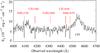 |
Fig. 1 SDSS spectrum of the zem = 1.94 QSO J 0815+2640. The C i λλ1560,1656 absorption lines detected at z = 1.681 are indicated, along with the presence of several low-ionization metal lines at the same redshift. Among the latter, the simultaneous detections of Si ii λ1526 and Al ii λ1670 lines were required by our detection algorithm to minimize the probability of coincidence. In this system, relatively weak Fe ii λ1608 absorption is also observed. |
The search for C i lines was limited to the regions of the spectra redwards of the QSO Lyman-α emission line to avoid the spurious coincidences that are frequent in the Lyman-α forest. The wavelength range above 7200 Å was also not considered in the search to avoid regions of the spectra that are heavily affected by residuals from the sky emission-line subtraction. We requested that the search window encompasses the wavelengths of the Si ii λ1526 and Al ii λ1670 absorption lines of the putative C i systems so that the validity of a system does not rely solely on the detection of two transitions (see above). For a given line of sight, the redshift lower bound (zmin) of the C i search is therefore the highest value between z = 3820/1526−1 ≃ 1.50 and (1 + zem) × 1215/1526−1 ≃ 0.8 × zem−0.2, where zem is the QSO emission redshift. The redshift upper bound (zmax) of the search is the lowest value between zem + 0.1 (to not exclude a priori proximate systems with infalling velocities of up to +5000 km s-1) and z = 7200/1656−1 ≃ 3.35. In order to avoid too many false positives at a low signal-to-noise ratio (S/N), we requested the median S/N per pixel to be higher than four for a given spectrum to be actually scanned. This resulted in a sample of 41 696 QSOs with 1.5 <zem< 4.46 whose spectra were searched for intervening or proximate C i absorbers. We did not initially reject broad absorption-line (BAL) quasars because our procedure follows the QSO continuum locally and can detect narrow absorption lines embedded in broad and not-fully-saturated troughs. Regions of deep absorption are avoided de facto when we study the number of intervening C i absorbers per unit redshift in Sect. 3.3 because they have low S/N per pixel.
Table 1 summarises our C i sample, which we refer to in the following as the overall sample. QSO names with J 2000 coordinates are given for each absorber. No line of sight is found to feature more than one system1. The SDSS plate and fibre numbers, as well as the MJD, are also provided in the table as useful cross-references. The QSO emission redshifts derived by the SDSS team are indicated, together with the absorption redshifts and rest-frame equivalent widths of the C i lines. The last were carefully determined by us for each individual system. In the next column of the table, we specify the average S/Ns per pixel in the regions the two C i lines are detected. At zabs> 2.2, the Lyman-α line of the systems is also covered by the SDSS spectra. We therefore provide in the table a determination of the total neutral atomic-hydrogen column density of these systems following the method developed by Noterdaeme et al. (2009b). The reliability of the latter is confirmed in a number of cases with follow-up high-resolution VLT/UVES spectroscopy (see the last column of Table 1, and Sect. 5). This column also has N(H i) measurements from UVES for several low-redshift systems for which Lyman-α absorption is not covered in the SDSS spectrum.
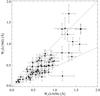 |
Fig. 2 Rest-frame equivalent widths of C i absorption lines measured in SDSS spectra and associated 1σ uncertainties. The upper dashed line shows the 1:1 relation expected in case of heavily saturated profiles. The lower dashed line shows the expectation for absorption lines on the linear part of the curve of growth. |
C i systems identified in SDSS-DR7 QSO spectra.
3. Sample properties
It must be noted that in this survey C i systems are found without any presumptions on the presence of neutral atomic hydrogen; i.e., the C i systems found in this work do not necessarily have to be DLAs. Moreover, DLA absorbers can be observed in SDSS spectra only when their redshifts are higher than 2.2, while C i lines can be identified down to zabs ≃ 1.50. As stated before, the reality of the identified C i systems in our sample was checked by visual inspection. Therefore, we believe the C i detections are secure. We discuss the completeness of our survey in Sect. 3.2.
3.1. Line equivalent widths
Because we rely on them in the analysis, we here seek to verify the robustness and accuracy of the equivalent-width measurements of C i-absorption lines performed in SDSS spectra. For this purpose, we plot in Fig. 2 the measured rest-frame equivalent widths of the C i λλ1560,1656 lines versus each other. It appears that except in one case, the strengths of the two lines are in the expected range. This gives confidence in the derived values and their associated uncertainties. In the case of the outlier seen in the lower part of the plot (i.e., at zabs = 1.526 towards SDSS J 125552.60+223424.4), an unrelated blend to the λ1656 line is a probable reason for the observed deviation.
All the systems are located within about 2σ of the boundaries defined by the optically thin regime, on one hand, and the relation expected for heavily saturated profiles, on the other. We note that because of their large equivalent widths (Wr ≳ 0.4 Å), most of the absorbers, especially those with equivalent-width ratios consistent with the optically thin regime, are probably made of numerous velocity components.
Here, we assumed that the C i ground state is solely responsible for the absorption lines while in reality the absorption from the two fine-structure energy levels of the neutral-carbon ground state (3P1 and 3P2) could contribute mildly to the measured equivalent widths. However, this will affect the equivalent widths of both of the λ1560 and λ1656 lines in the same way so that any departure from the assumed relations due to this blending will be small.
3.2. Completeness
Before discussing the number of C i absorbers per unit redshift (nC i; see following section), we first need to estimate the completeness of the sample. Given the resolving power R of the SDSS spectra, the C i λ1560 line rest-frame equivalent width limit is given by 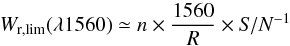 (1)where n = 2 is the number of standard deviations above which the peak absorption must be detected and S/N> 4 is the limit on the S/N per pixel at the corresponding line position. The FWHM of the lines is sampled by two velocity pixels with constant values. Our survey should therefore be complete down to Wr,lim(λ1560) ≃ 0.4 Å.
We checked the exact level of completeness of our survey at this equivalent-width limit by implementing the following procedure. For this purpose, we used the same data set that we used for calculating nC i in Sect. 3.3, i.e., the same quasar sample, the same [zmin,zmax] values, and the same mean S/N> 4 limit. We then randomly selected 1000 QSO spectra and introduced an artificial C i system of rest-frame equivalent width Wr(λ1560) at different positions in the spectra where the local S/N at both C i lines is greater than four. The distribution of the equivalent width ratio of the λ1560 and λ1656 lines is assumed to be a normal distribution with a dispersion corresponding to what is seen in Fig. 2. However, neither the equivalent width ratio nor the exact number of artificial systems used in the simulation has any significant impact on the completeness we infer.
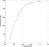 |
Fig. 3 Completeness of our C i search as a function of C i λ1560 rest-frame equivalent width. Each point is based on a total of 40 000 artificial C i systems introduced in 1000 randomly selected SDSS QSO spectra. The vertical line shows our chosen completeness limit of Wr(λ1560) = 0.4 Å. |
We implemented about 40 000 C i systems that we sought to recover by using the same automatic procedure as described in Sect. 2. We varied Wr over the range 0.1–1.0 Å and defined the completeness as the ratio of the number of recovered systems to the total number of systems introduced in the spectra. The results are displayed in Fig. 3. It can be seen that the completeness is greater than 80% for Wr(λ1560) ≥ 0.4 Å.
3.3. Number of absorbers per unit redshift
We calculated the sensitivity function, g(z), of our survey, i.e., the number of lines of sight that probe a given redshift z and that have S/N> 4 at the expected positions of both C i lines. This function is shown in Fig. 4. It combines the [zmin,zmax] pairs, previously defined in Sect. 2, for all the lines of sight. We further excluded the regions with velocities relative to the QSO emission redshifts lower than 5000 km s-1, which could, in principle, be influenced by the quasar (see Sect. 3.4). The uncertainties on zem are of the order of 500 km s-1 (see, e.g., Pâris et al. 2012) and are therefore small enough not to affect the statistics. The total statistical absorption path length probed by the QSO sample over z = 1.50−3.35 is Δz ≈ 13 000 with an average redshift ⟨z⟩ = 1.9. From Fig. 4, it is apparent that the sensitivity of the survey is an increasing function towards lower redshifts. One therefore expects a larger number of absorbers to be found at z< 2. This is what is observed in practice as indicated by the redshift histogram of the detected intervening C i absorbers over-plotted in the same figure. On the other hand, the small number of C i systems found at zabs> 2.2 (i.e., eight systems out of a total of 66 systems or, equivalently, 12% of the sample) is striking.
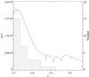 |
Fig. 4 Statistical sensitivity function of our C i survey, g(z) (solid curve; left-hand axis). The dips seen at z ~ 2.35 (resp. 2.6) are caused by C i λ1656 (resp. C i λ1560) falling over bad pixels at the junction between the two SDSS CCD chips. Dips at higher redshifts (z ~ 2.8,3.05) are due to telluric lines (e.g., [O i] λ6300). The histogram (right-hand axis) shows the C i-absorber number counts in different redshift bins for intervening systems with rest-frame equivalent width above our completeness limit, i.e., Wr(λ1560) ≥ 0.4 Å. |
Intervening C i-absorber number counts.
To investigate this further, we calculated the number of intervening C i absorbers per unit redshift, nC i, in two redshift bins of roughly equal total absorption path length (with boundary redshift z = 1.9). Here, we only considered the systems with rest-frame equivalent widths above the completeness limit of the survey, i.e., Wr(λ1560) ≥ 0.4 Å. The results are summarized in Table 2 and shown in Fig. 5. In the table, we also separated the strongest from the weaker absorbers (around a median rest-frame equivalent width of 0.64 Å) but there is no obvious difference between the redshift evolution of these two groups.
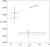 |
Fig. 5 Evolution of the number of intervening C i absorbers per unit redshift, nC i, for systems with rest-frame equivalent widths Wr(λ1560) ≥ 0.4 Å. The measurements (solid) are corrected for incompleteness at the latter limit. For clarity purposes, the uncorrected data (dashed) are displayed with a slight offset in abscissa. The curve shows the expected redshift behaviour of a non-evolving population. |
The nC i ~ 1.4 × 10⁻³ we measure in the higher redshift bin (1.9 <zabs< 3.35), taking the effect of incompleteness estimated in Sect. 3.2 into account, implies that C i systems with Wr(λ1560) ≥ 0.4 Å are more than one hundred times rarer than DLAs at zabs = 2.5 (see Noterdaeme et al. 2012). An evolution of nC i, with nearly thrice as many systems below z = 1.9 than above that is also observed. Compared to the redshift behaviour of a non-evolving population, this is significant at the 4.3σ level. Such an evolution is interesting and should be studied further since it depends on the balance between dust shielding and the UV radiation field. This may imply a strong evolution of the shielding of 10 eV photons by dust between z = 2.5 and z = 1.5.
3.4. Proximate systems
There are 14 C i systems with velocities relative to the QSO emission redshifts that are lower than 5000 km s-1. These could be associated with the QSO host galaxy or nearby environment. Six systems even have absorption redshifts greater than the corresponding QSO emission redshifts (by up to ~4000 km s-1), which is difficult to explain by high peculiar velocities in intervening systems. Imposing the same data-quality cuts and minimum equivalent widths as in the previous section, we find that the incidence of C i absorbers at small velocity differences from the quasars is consistent with that of intervening systems. However, associated errors are large due to small number statistics.
Because of the clustering of galaxies around the massive QSO host galaxies, an excess of proximate C i systems could be expected. However, C i is a fragile species that can easily be photo-ionized by the intense UV radiation emitted by the QSO engine. Interestingly, the lack of a significant excess of proximate systems was also observed by Prochaska et al. (2008) when considering DLAs. In this case, the abundance of proximate DLAs is only a factor of two larger than that of the overall DLA population. A similarly low over-abundance factor was observed by Finley et al. (2013) for strong DLAs with log N(H i) > 21.3 (atoms cm-2). This is much less than expected based on clustering arguments alone.
In this work, we do not observe that the properties of proximate C i systems are different from those of intervening C i systems. This is true for redshift, C i equivalent-width, H i content, reddening, and UV bump-strength distributions. Nevertheless, because of the possibly different origins of these absorbers and the possible requirement of strong dust shielding from the nearby QSOs, we distinguish in the following proximate C i systems from the rest of the population and comment, whenever possible, on proximate C i systems of interest.
4. Evidence of dust
4.1. QSO optical colours
To assess the impact of the C i absorbers on their background QSOs and check for the existence of dust in these systems, we first consider the observed colours of these QSOs and compare them with the colours of the overall QSO population used as a control sample.
In Fig. 6, we show the distributions of (g−r), (r−i), and (r−z) colours for the 41 696 QSOs whose spectra were searched for C i absorption. In the upper panels of this figure, it is apparent that the lines of sight with detected C i absorption do not distribute in the same way as the other lines of sight. They are all displaced together towards redder optical colours compared to the average loci of the QSO redshift sequences. The effect is most easily seen in the lower panels of Fig. 6, which compare the colour histograms of the two QSO populations (i.e., the C i-detected QSO sample and the overall QSO sample). The two-sided Kolmogorov-Smirnov test probability that the two samples are drawn from the same parent distribution is as low as ≲10-10. The typical colour excess is ~0.15 mag, i.e., about five times more than the mean (r−z) colour excess of 0.03 mag derived by Vladilo et al. (2008) in zabs ≈ 2.8 DLAs from SDSS DR 5. A similar result for DLAs was found by Khare et al. (2012) based on (g−i) colours of SDSS-DR 7 QSOs. This is clear evidence for the presence of dust among C i absorbers.
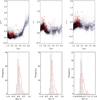 |
Fig. 6 Upper panels: colours of the 41 696 SDSS QSOs whose spectra were searched for C i absorption versus QSO emission redshift. (g−r), (r−i) and (r−z) colours are displayed in the left-, middle-, and right-hand panels, respectively. The thick blue line shows the median QSO colour as a function of redshift. Thin blue lines show one standard deviation away from that median. The red circles indicate the 66 lines of sight passing through C i-detected gas. Lower panels: distribution of colour excesses (defined as, e.g.: (g−r)−⟨g−r⟩zQSO for Δ(g−r)) for the 66 QSOs whose spectra were found to exhibit C i absorption (thick red histogram) compared to the whole QSO sample (thin-hashed histogram, scaled down by a factor of 632 to have the same area). In each panel (from left to right: Δ(g−r), Δ(r−i) and Δ(r−z)), vertical dotted red lines indicate the median colour excesses of the sample of QSOs with detected C i absorption. The median values for the whole QSO sample are shown by vertical dashed lines. |
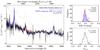 |
Fig. 7 Left-hand panel: illustration of reddening measurement based on QSO SED fitting. The blue curve shows our best fit to the QSO continuum using the QSO template spectrum from Vanden Berk et al. (2001) and the best-fitting LMC extinction law at the redshift of the C i absorber. The non-extinguished QSO template is displayed in grey. The additional presence of a 2175 Å absorption feature is shown by the light-red shaded area (i.e., Abump). The broken orange line at zero ordinate indicates the wavelength regions devoid of QSO emission lines, strong absorption lines and sky residuals, that were used during the χ2 minimization. Upper right-hand panel: distribution of reddening measured in the QSO control sample assuming either a SMC (red) or the best-fitting extinction law (in this case, LMC; blue). The reddening values of the line of sight under consideration are indicated by downward arrows. Lower right-hand panel: same as above but for the distribution of 2175 Å bump strengths. |
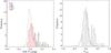 |
Fig. 8 Left-hand panel: histogram of reddening for the sample of 66 QSOs whose spectra were found to exhibit C i absorption (multi-colour). The colour/hash coding for the different C i-detected lines of sight relates to the best-fitting extinction law (red: SMC; blue: LMC; green: LMC2; purple: MW). The distribution of reddening from the QSO control sample (C.S.), i.e., the sum of the normalized distributions of individual QSO control samples, is displayed with dashed lines. Right-hand panel: same as in the left-hand panel but for the histogram of 2175 Å bump strengths. The distribution from the QSO control sample is well represented by a Gaussian profile (solid curve). |
4.2. Reddening
Motivated by the unequivocal signature of dust in the form of a colour excess of the background QSOs with detected C i absorption, we now aim at constraining the properties and the nature of dust in these systems.
For each of the 66 QSOs with foreground C i absorbers, we derived the QSO reddening, E(B−V), following the same approach as used in Srianand et al. (2008a) and Noterdaeme et al. (2009a, 2010a), for example. First, we corrected the QSO spectra for Galactic reddening using the extinction maps from Schlegel et al. (1998). We then fitted the spectra with the SDSS QSO composite spectrum from Vanden Berk et al. (2001) shifted to that QSO emission redshift and reddened with either a Small Magellanic Cloud (SMC), Large Magellanic Cloud (LMC), LMC2 super shell, or Milky Way (MW) extinction law (Gordon et al. 2003) at the C i-absorber redshift. Our procedure is illustrated in the left-hand panel of Fig. 7. The fit with the lowest χ2 value indicates the most representative extinction law for a given absorber. The latter is specified in column “Best fit” of Table 3, and the corresponding E(B−V) value is given in the preceding column.
For each QSO line of sight exhibiting C i absorption, we defined a control sample (hereafter denoted as “C.S.”) made of SDSS-DR 7 QSOs from the searched sample having an emission redshift within ± 0.05 and a z-band magnitude within ± 0.1 mag from those of the QSO under consideration. In some instances, this resulted in a sample of less than 30 QSOs in which case we increased the above maximum magnitude difference by steps of 0.01 until the number of QSOs in the control sample reached (or exceeded) 30. We then applied the exact same fitting procedure as described in the previous paragraph to each QSO spectra from the control sample. Table 3 lists the number of QSOs and the median reddening and standard deviation of the distribution of E(B−V) values in each control sample (see the upper right panel of Fig. 7 for an illustration). The values given in Table 3 correspond to the most representative extinction law previously determined for that particular C i-detected QSO spectrum.
In the left-hand panel of Fig. 8, we show the histogram of reddening for the sample of 66 QSO lines of sight with detected C i absorbers compared to the cumulative control sample (calculated as the sum of the normalized distributions of individual control samples). As in Sect. 4.1, an offset between the two samples is apparent. The mean reddening induced by C i systems is 0.065 mag. A tail in the histogram of the C i-detected lines of sight is observed with E(B−V) values up to ~0.3 mag.
4.3. The 2175 Å extinction feature
A number of C i-detected QSO spectra are best matched by an extinction law exhibiting the absorption feature at rest-frame wavelength 2175 Å. To measure the strength of this UV bump (denoted Abump), we followed a prescription similar to the one used by Jiang et al. (2010) where the observed QSO spectrum was fitted with the SDSS QSO composite spectrum reddened via a parametrized pseudo-extinction law made of a smooth component and a Drude component. However, here we fixed the wavelength and width of the bump to the Galactic values determined by Fitzpatrick & Massa (2007). Both of these quantities indeed show little variation from line of sight to line of sight through the Galaxy and the Magellanic Clouds. This then limits the number of free parameters and prevents the fit from diverging towards very wide and shallow solutions that could be non-physical. Indeed, imperfect matching of the observed QSO continuum by the smooth component is expected owing to intrinsic QSO-shape variations (e.g., Pitman et al. 2000).
The fitting process is illustrated in the left-hand panel of Fig. 7. The shaded area represents the measure of the bump strength. This is the difference between the above best-fit function and the same function but considering only its smooth component (i.e., with the Drude component set to zero). The Abump values are listed for each absorber in Table 3. As previously done for determining reddening (see Sect. 4.2), we also defined a QSO control sample whose measured Abump distribution is shown in the lower right-hand panel of Fig. 7 (i.e., for the given QSO emission redshift and z-band magnitude). Table 3 gives the median and standard deviation of this distribution for each control sample.
The histogram of bump strengths in the C i-absorber sample is displayed in the right-hand panel of Fig. 8. One can see from this figure that more than a quarter of the C i systems feature absorption at 2175 Å. This strengthens the result from the previous section that significant reddening of the background QSOs by dust is induced by some of the C i absorbers. We come back to this and quantify the effect in Sect. 6.
In the following, we use the median E(B−V) and Abump values of the control samples, i.e., ⟨ E(B−V) ⟩ C.S. and ⟨ Abump ⟩ C.S., to define the exact colour excess and bump strength towards a given C i-detected QSO line of sight: E(B−V) = E(B−V)measured− ⟨ E(B−V) ⟩ C.S., and likewise for Abump. These zero-point corrections are usually almost negligible (see Table 3). In addition, the standard deviations of E(B−V) and Abump values in each control sample provide an estimate of the uncertainty due to intrinsic QSO-shape variations (see Pitman et al. 2000), hence the significance of the reddening induced by each C i absorber and the significance of associated 2175 Å absorption, respectively.
SED fitting of QSO spectra with detected C i absorbers.
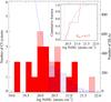 |
Fig. 9 Neutral atomic-hydrogen column-density distribution of C i absorbers (red-filled histogram; left-hand axis). Proximate systems are displayed in salmon. The N(H i) distribution of intervening DLAs from SDSS DR7 (Noterdaeme et al. 2009b, blue-hashed histogram) is over-plotted using a different scaling (right-hand axis) so that the areas of the two histograms above log N(H i) = 20.3 are equal. The curve is a fit of the distribution in the sub-DLA regime from Prochaska et al. (2014). The inset shows the cumulative N(H i) distributions of the intervening C i and DLA samples starting at log N(H i) = 20.3 (atoms cm-2) and the two-sided Kolmogorov-Smirnov test probability that the two distributions come from the same parent population. |
5. H i content
As part of a spectroscopic campaign, which we will describe in a companion paper, we followed up the C i absorbers from the overall sample that are observable from the southern hemisphere using VLT/UVES. We present in Fig. 9 the H i column-density distribution of this C i-absorber subsample (referred to in the following as the H i subsample) and compare it with the distribution of N(H i) from systematic DLA and/or sub-DLA surveys.
We secured H i column-density measurements for most of the systems in the overall sample that have a declination of δ< + 28deg: i.e., 14 out of 16 systems at redshifts zabs> 1.8 (the two exceptions being the lines of sight towards SDSS J 091721.37+015448.1 and J 233633.81−105841.5) and four out of eight systems at zabs ≈ 1.75 (see Table 1). While H i column densities derived from UVES spectroscopy are usually more accurate, the last two columns of Table 1 show that they confirm those derived directly from SDSS spectra as seen from the five systems at zabs> 2.2 where this measurement could be done from both datasets. For this reason, we complement our UVES measurements with the values we derived using SDSS spectra for the three systems at zabs> 2.2, for which high-resolution spectroscopic data are not available because the background QSOs are too far north for the VLT to observe them. The H i subsample thus comprises a total of 21 systems.
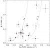 |
Fig. 10 C i λ1560 rest-frame equivalent width versus N(H i), the neutral atomic-hydrogen column density of C i absorbers. Intervening (resp. proximate) systems are displayed as filled (resp. empty) black circles. Data points are circled in red as they correspond to the subsample of C i systems with measured N(H i), i.e., the H i subsample. The dashed (resp. dashed-dotted) curve materializes the limit above which systems are expected to have a metallicity larger than one-tenth of solar (resp. in excess of solar; see text). The completeness limit of the survey is indicated by the horizontal line. |
In Fig. 9, we compare the observed H i column-density distribution of C i-selected absorbers with that of H i-selected DLAs (from SDSS DR 7 as well; Noterdaeme et al. 2009b). In this figure, we also show the expected number of sub-DLAs using the fitted distribution function from Prochaska et al. (2014). We find that a large number of C i absorbers have neutral atomic-hydrogen column densities slightly below the conventional DLA limit (N(H i) = 2 × 10²⁰ atoms cm-2) and are therefore classified as strong sub-DLAs. However, the number of C i absorbers among sub-DLAs is much less than among DLAs, indicating that efficient shielding is much more difficult to obtain below the DLA limit. Though rare, the existence of C i absorbers with low neutral atomic-hydrogen column densities supports the presence of dust in these systems. The dust-to-gas ratio in these systems has to be high enough so that the absorption of UV photons by dust allows C i to be present in large amounts.
No C i system is found with log N(H i) < 19 (atoms cm-2). This is a regime where shielding of UV photons becomes extremely difficult even in the presence of dust. However, it is possible that such systems are missed in our search. Indeed, as seen in Fig. 10, there is a tendency for neutral atomic-hydrogen column density to increase with C i equivalent width. The gradually decreasing completeness fraction of the survey below Wr(λ1560) ≈ 0.4 Å (see Sect. 2) would therefore preclude low N(H i) systems from appearing in our sample.
Above the DLA limit, where the incompleteness of our survey is less of a problem, it appears that C i-selected absorbers do not follow the statistics of H i-selected DLAs. Although there are only nine C i systems with log N(H i) > 20.3 (atoms cm-2), it is apparent that the overall N(H i) distribution of C i systems is relatively flat. A two-sided Kolmogorov-Smirnov test applied to all absorbers with log N(H i) > 20.3 (atoms cm-2) gives a probability of only 17% that the two distributions come from the same parent population (see inset of Fig. 9). This could be explained by a larger number of velocity components in higher H i column-density gas, thereby increasing the probability of detecting C i. Moreover, large amounts of shielded gas are probably the consequence of the line of sight passing through the absorbing galaxy at a low impact parameter, in which case we can expect the N(H i) distribution to be flatter than for the overall DLA population.
The strongest DLA found among the C i absorbers in the H i subsample has N(H i) = 1021.8 atoms cm-2. It is, however, located at zabs ≈ zem. Even ignoring proximate systems, it is still surprising that three intervening DLAs with N(H i) ≥ 1021 atoms cm-2 are present in such a small absorber sample. From DLA statistics alone, the probability of randomly selecting three DLAs that are that strong in a sample of six DLAs is only 6%. There is therefore a probable excess of strong DLAs amongst C i absorbers. While the dust content of these systems is significant (see Sects. 4.1 and 4.2), their dust-to-gas ratio must be limited. Indeed, dust reddening and extinction of the background QSOs will inevitably reduce the incidence of strong and dusty DLAs in magnitude-limited QSO samples. This implies that the actual proportion of strong DLAs amongst C i systems in general is likely to be even higher than what we found.
6. Empirical relations in the sample
Based on the results presented in the previous sections, we now study the empirical relations between the different quantities measured in this work: neutral atomic-carbon and neutral atomic-hydrogen contents, the reddening that C i-selected absorbers induce on their background QSOs, and the strength of possible 2175 Å extinction features. Because the C i λ1560 transition line is weaker, so it exhibits less saturation than C i λ1656, we adopted the equivalent width of the former as a proxy for the amount of neutral atomic carbon in the systems.
In Fig. 10, we plot the C i λ1560 rest-frame equivalent width versus log N(H i) for the C i absorbers from the H i subsample. Both quantities appear to be weakly correlated. A Kendall rank-correlation test indicates that the significance of the correlation is only 1.8σ. There is therefore a tendency for strong DLAs to have larger C i equivalent widths, but at the same time, for a given H i column density, the C i content can vary substantially from one system to another. High values of Wr(λ1560) are observed in DLAs but also in sub-DLAs. The amount of shielded and probably cold gas could actually be large in some of these sub-DLAs. From the optically thin approximation applied to the C i λ1560 absorption line and assuming the ionization equilibrium relation, N(C i)/N(C ii)~ 0.01, which is valid for the cold neutral medium (CNM; see, e.g., Jenkins & Tripp 2011), a lower limit on the gas metallicity can be derived: ![Mathematical equation: \begin{equation} \label{eq:met} [\mathrm{X}/\mathrm{H}]\ga 18.35+\log\left(\frac{W_\mathrm{r}(\lambda 1560)}{0.01 \times N(\ion{H}{i})}\right) \cdot \end{equation}](/articles/aa/full_html/2015/08/aa24122-14/aa24122-14-eq299.png) (2)For Wr(λ1560) = 0.4 Å and log N(H i) = 20 (atoms cm-2), the metallicity should be close to solar. More generally, the curves in Fig. 10 were calculated using the above equation and assuming metallicities of one-tenth of solar and solar. Within measurement uncertainties, most of the C i systems lie in between these two curves. If the medium probed by the line of sight is a mixture of cold and warm gas, the metallicity of the systems will be even higher. However, if part of the hydrogen is in molecular form, the metallicity will be lower. For the whole C i-absorber sample, Eq. (2) implies a metallicity distribution ranging between [X/H] =−1.4 and metallicities in excess of solar with a median value of [X/H] ≈−0.5. This means that the metallicities of C i absorbers would on average be at least ten times greater than those of typical DLAs (for the latter, see, e.g., Rafelski et al. 2012). This should be confirmed by accurate measurements of metal column densities.
(2)For Wr(λ1560) = 0.4 Å and log N(H i) = 20 (atoms cm-2), the metallicity should be close to solar. More generally, the curves in Fig. 10 were calculated using the above equation and assuming metallicities of one-tenth of solar and solar. Within measurement uncertainties, most of the C i systems lie in between these two curves. If the medium probed by the line of sight is a mixture of cold and warm gas, the metallicity of the systems will be even higher. However, if part of the hydrogen is in molecular form, the metallicity will be lower. For the whole C i-absorber sample, Eq. (2) implies a metallicity distribution ranging between [X/H] =−1.4 and metallicities in excess of solar with a median value of [X/H] ≈−0.5. This means that the metallicities of C i absorbers would on average be at least ten times greater than those of typical DLAs (for the latter, see, e.g., Rafelski et al. 2012). This should be confirmed by accurate measurements of metal column densities.
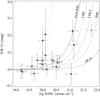 |
Fig. 11 Reddening of the background QSOs with detected C i absorption versus N(H i) of the C i absorbers. Symbol conventions are the same as in Fig. 10. The solid curve shows the relation observed in the local ISM where E(B−V) /N(H)= 1.63 × 10⁻²² mag atoms-1 cm2 (Gudennavar et al. 2012). The dotted curve illustrates a reddening per hydrogen atom ten times higher than that. The dashed curves correspond to the observations of the Magellanic Clouds (Gordon et al. 2003). The long-dashed curve shows the relation derived for typical DLAs at zabs ≈ 2.8 (e.g., Vladilo et al. 2008; Khare et al. 2012). |
In Fig. 11, we display the relation between E(B−V) and log N(H i) among the C i absorbers from the H i subsample. Here again, the data points are highly scattered. Most of the systems are associated with low, albeit consistently non-zero, QSO reddening. Since most of the N(H i) values are relatively low, the measured amounts of reddening, with median E(B−V) ~ 0.045, are actually remarkable. This departs from what is observed in the overall DLA population where the reddening is usually negligible (see, e.g., Vladilo et al. 2008; Khare et al. 2012). Vladilo et al. (2008) have shown that DLAs at zabs ≈ 2.8 typically induce a reddening E(B−V) ~ 5 × 10⁻³ mag. Apart from a few outliers, most of the C i systems have reddening properties that are consistent with those of the Galactic ISM. This is represented in Fig. 11. In the Galaxy, the reddening induced along a line of sight is indeed directly proportional to the neutral atomic-hydrogen column density with E(B−V) /N(H)= 1.63 × 10⁻²² mag atoms-1 cm2 (Gudennavar et al. 2012). Only two C i systems with large N(H i) are more consistent with what is seen in typical DLAs and/or along SMC lines of sight, where the above ratio is lower than in the Galaxy. Two other C i systems with low N(H i) might also deviate from the Galactic relation being consistent with a ten-times higher ratio. We caution, however, that the uncertainties on the reddening measurements are fairly large. If real, this would imply in the latter systems the existence of a grain chemistry more evolved than in the Galaxy with a higher ratio of big grains to very small grains (e.g., Pei 1992). This is opposite to the trend observed in the Magellanic Clouds. In such systems, strong 2175 Å absorption is expected. Interestingly, this is what is observed in practice because these two C i systems exhibit two of the strongest three Abump values of the H i subsample.
To investigate the characteristics of the C i absorbers further, we look in Fig. 12 in more detail at the properties of dust in these systems. In the left-hand panel of this figure, E(B−V) and Wr(λ1560) are found to be correlated with each other at the 4.4σ significance level. This is noteworthy because different degrees of saturation of the C i λ1560 line are expected to produce scatter in this relation. This implies that the neutral-carbon content of the C i systems is intimately related to the reddening induced along the line of sight or, equivalently, that the amounts of shielded gas and dust are tightly inter-connected. We also note that two of the highest three E(B−V) values in this plot correspond to systems located at zabs ≈ zem. This may, however, be the result of the small sample size because the reddening induced by the other proximate systems in our sample varies substantially from one system to another.
The relation between E(B−V) and the UV bump strength, Abump, which we previously determined independently from E(B−V) (see Sect. 4.3), is shown in the right-hand panel of Fig. 12. It can be seen that both quantities are tightly correlated (6.0σ). A linear least-squares fit (linear correlation coefficient of r = 0.77), taking errors in both parameters into account, gives E(B−V) ≃ 0.43 × Abump. The 2175 Å extinction feature is detected at more than 2σ (95% confidence level) in about 30% of the C i systems. In such cases, we find Abump ~ 0.4 and E(B−V) ~ 0.2 mag or, equivalently, AV ~ 0.6 mag. These values are comparable to what Budzynski & Hewett (2011) have found when targeting the strongest Mg ii systems from SDSS DR 6 [1 <Wr(λ2796) < 5 Å] where the 2175 Å absorption is detected on a statistical basis alone (see also Jiang et al. 2011, for candidate 2175 Å absorption in similar systems). Interestingly, our measured UV bump strengths are also comparable to what has been observed along GRB lines of sight at similarly low levels of extinction, e.g., towards GRB 080605 (see Zafar et al. 2012).
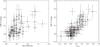 |
Fig. 12 Left-hand panel: reddening of the background QSOs with detected C i absorption (overall sample) versus C i λ1560 rest-frame equivalent width. Symbol conventions are the same as in Fig. 10. The data points circled in red correspond to the H i subsample. Right-hand panel: same as in the left-hand panel with the exception that reddening is plotted against the 2175 Å bump strength. |
In the local Universe, 2175 Å absorption can be observed with reddening values as low as ~0.2 mag (see, e.g., Fitzpatrick & Massa 2007). Even at such low levels of reddening, the UV bump is significantly stronger along Galactic lines of sight, i.e., by up to a factor of ten, than in the present C i absorber sample and/or through GRB host galaxies. This discrepancy may be explained if these high-redshift systems probe regions of the ISM affected by a star formation that is more vigorous than in the Galaxy. A similar argument was proposed by Gordon et al. (2003) with the aim of explaining the variety of LMC and SMC extinction curves. In fact, most of the C i absorbers at the high end of the reddening tail in our sample are best-fit using the extinction law of the LMC2 super-shell near the 30 Dor star-forming region2 (see left panel of Fig. 8). This means that the far-UV rise of the extinction curve is enhanced and the carriers of the 2175 Å absorption are depleted compared to Galactic lines of sight. This is probably the consequence of a high UV flux and/or the mechanical feedback from stars (e.g., Fischera & Dopita 2011) in the vicinity of the C i systems. In contrast, the lack of a UV bump in typical DLAs (e.g., Khare et al. 2012) is probably intrinsic to their low dust and metal contents since the lines of sight are likely to pass at high impact parameters from the absorbing galaxy.
The main outlier in the right-hand panel of Fig. 12, which exhibits high reddening but no UV bump, is a proximate system. This is consistent with the above picture where the enhanced UV radiation field from the QSO and/or star-forming regions within the QSO host galaxy are expected to deplete the carriers of the 2175 Å absorption.
7. Conclusions
In this work, we presented a new population of QSO absorbers that was selected directly from the properties of the shielded gas, namely the strongest C i absorbers, detected in low-resolution QSO spectra from the SDSS-II DR 7 database. These C i absorbers, with Wr(λ1560) ≥ 0.4 Å, are more than one hundred-times rarer than DLAs at zabs = 2.5. Their number per unit redshift is increasing significantly below zabs = 2, probably coupled to an increase in the star-formation efficiency at these redshifts. Gupta et al. (2012) report a similarly high detection rate of 21-cm absorbers towards even lower redshifts among strong Mg ii systems, which they argue must be related to the evolution of the CNM filling factor in the latter systems.
The H i column-density distribution of C i-selected absorbers is flatter than that of H i-selected absorbers. While sub-DLAs have a much larger cross-section than DLAs, this can be understood as the shielding of the gas being more difficult at low H i column densities and there are probably fewer clouds along the line of sight. Cold and dusty gas as traced by C i absorbers is also more likely to be found at low impact parameters from the absorbing galaxies where a flatter N(H i) distribution is expected. Indeed, despite a likely bias against strong DLAs with large amounts of dust, we find there is a probable excess of strong DLAs with log N(H i) > 21 (atoms cm-2) among C i systems compared to systematic DLA searches. This is reminiscent of the N(H i) distribution of DLAs within GRB host galaxies, which is skewed towards extremely strong DLAs (see Fig. 10 in Fynbo et al. 2009).
The reddening and therefore the presence of dust along the QSO lines of sight with detected C i absorption is directly related to the amount of shielded gas but depends weakly on the total H i column density. The latter can indeed vary by more than a factor of ten for the same C i rest-frame equivalent width. This is probably the consequence of the shielded gas being clumpy, while H i absorption samples simultaneously warm diffuse neutral clouds and cold, high-metallicity dusty pockets of gas. The presence of dust inducing significant reddening of the background QSOs and/or 2175 Å extinction features is ubiquitous in about 30% of the C i absorbers. Several systems like these have been found before (see, e.g., Srianand et al. 2008a; Wang et al. 2012). Here, we find that the UV bump is weak compared to Galactic lines of sight exhibiting the same amount of reddening. We interpret this as the consequence of star formation in the vicinity of the systems.
It is likely that the metal and molecular contents of C i absorbers are high and actually higher than those of most DLAs studied until now. High-resolution spectroscopic follow-up observations of the present sample therefore opens up the door to systematic searches for carbon monoxide (CO; see Noterdaeme et al. 2011) and molecules like CN and CH, as well as for diffuse interstellar bands at high redshift. Such a spectroscopic campaign will be presented in a companion paper. The typical reddening induced by C i absorbers along with the relation between reddening and shielded-gas column density imply that the extinction could be high in some DLAs with C i absorption. If strong dusty DLAs exist, they probably have been missed in the current magnitude-limited QSO samples (see also Boissé et al. 1998; Vladilo et al. 2008). Some of the QSO lines of sight identified here, as well as those that may be found by extending the present survey to even larger databases3, will result in exceedingly long integration times on high-resolution spectrographs installed on 8−10 m class telescopes. These will, however, be targets of choice for the coming generation of extremely large telescopes.
There is, however, a second C i system towards SDSS J 234023.67− 005327.1, which with zabs = 1.36, falls below the redshift cut-off of our survey. This system happens to be detected in 21-cm absorption so is also related to cold gas (see Gupta et al. 2009; Kanekar et al. 2010).
Super-giant shells with sizes approaching 1 kpc form the largest structures seen in the ISM of galaxies where large amounts of kinetic energy are contributed by multiple supernovae explosions and energetic stellar winds.
From the Baryon Oscillation Spectroscopic Survey, which is part of SDSS-III, relatively few additional C i systems are expected since the bulk of the new QSOs is at zem ~ 3, which provides shorter C i-absorption path length.
Acknowledgments
P.N. acknowledges support from the ESO Chile visiting scientist programme. R.S. and P.P.J. gratefully acknowledge support from the Indo-French Centre for the Promotion of Advanced Research (Centre Franco-Indien pour la Promotion de la Recherche Avancée) under contract No. 4304-2. The authors of this paper also acknowledge the tremendous effort put forth by the Sloan Digital Sky Survey team to produce and release the SDSS survey. Funding for SDSS and SDSS-II has been provided by the Alfred P. Sloan Foundation, the Participating Institutions, the National Science Foundation, the US Department of Energy, the National Aeronautics and Space Administration, the Japanese Monbukagakusho, the Max Planck Society, and the Higher Education Funding Council for England. The SDSS Web Site is http://www.sdss.org/. The SDSS is managed by the Astrophysical Research Consortium for the Participating Institutions. The Participating Institutions are the American Museum of Natural History, Astrophysical Institute Potsdam, University of Basel, University of Cambridge, Case Western Reserve University, University of Chicago, Drexel University, Fermilab, the Institute for Advanced Study, the Japan Participation Group, Johns Hopkins University, the Joint Institute for Nuclear Astrophysics, the Kavli Institute for Particle Astrophysics and Cosmology, the Korean Scientist Group, the Chinese Academy of Sciences (LAMOST), Los Alamos National Laboratory, the Max-Planck-Institute for Astronomy (MPIA), the Max-Planck-Institute for Astrophysics (MPA), New Mexico State University, Ohio State University, University of Pittsburgh, University of Portsmouth, Princeton University, the United States Naval Observatory, the University of Washington.
References
- Abazajian, K. N., Adelman-McCarthy, J. K., Agüeros, M. A., et al. 2009, ApJS, 182, 543 [NASA ADS] [CrossRef] [Google Scholar]
- Balashev, S. A., Petitjean, P., Ivanchik, A. V., et al. 2011, MNRAS, 418, 357 [NASA ADS] [CrossRef] [EDP Sciences] [PubMed] [Google Scholar]
- Balashev, S. A., Klimenko, V. V., Ivanchik, A. V., et al. 2014, MNRAS, 440, 225 [NASA ADS] [CrossRef] [Google Scholar]
- Boissé, P., Le Brun, V., Bergeron, J., & Deharveng, J.-M. 1998, A&A, 333, 841 [NASA ADS] [Google Scholar]
- Booth, R. S., de Blok, W. J. G., Jonas, J. L., & Fanaroff, B. 2009, ArXiv e-prints [arXiv:0910.2935] [Google Scholar]
- Budzynski, J. M., & Hewett, P. C. 2011, MNRAS, 416, 1871 [NASA ADS] [CrossRef] [Google Scholar]
- Duffy, A. R., Meyer, M. J., Staveley-Smith, L., et al. 2012, MNRAS, 426, 3385 [NASA ADS] [CrossRef] [Google Scholar]
- Finley, H., Petitjean, P., Pâris, I., et al. 2013, A&A, 558, A111 [Google Scholar]
- Fischera, J., & Dopita, M. 2011, A&A, 533, A117 [NASA ADS] [CrossRef] [EDP Sciences] [Google Scholar]
- Fitzpatrick, E. L., & Massa, D. 2007, ApJ, 663, 320 [NASA ADS] [CrossRef] [EDP Sciences] [Google Scholar]
- Fynbo, J. P. U., Jakobsson, P., Prochaska, J. X., et al. 2009, ApJS, 185, 526 [NASA ADS] [CrossRef] [Google Scholar]
- Ge, J., & Bechtold, J. 1999, in Highly Redshifted Radio Lines, eds. C. L. Carilli, S. J. E. Radford, K. M. Menten, & G. I. Langston, ASP Conf. Ser., 156, 121 [Google Scholar]
- Gordon, K. D., Clayton, G. C., Misselt, K. A., Landolt, A. U., & Wolff, M. J. 2003, ApJ, 594, 279 [NASA ADS] [CrossRef] [EDP Sciences] [Google Scholar]
- Gudennavar, S. B., Bubbly, S. G., Preethi, K., & Murthy, J. 2012, ApJS, 199, 8 [NASA ADS] [CrossRef] [Google Scholar]
- Gupta, N., Srianand, R., Petitjean, P., Noterdaeme, P., & Saikia, D. J. 2009, MNRAS, 398, 201 [NASA ADS] [CrossRef] [Google Scholar]
- Gupta, N., Srianand, R., Petitjean, P., et al. 2012, A&A, 544, A21 [NASA ADS] [CrossRef] [EDP Sciences] [Google Scholar]
- Jenkins, E. B., & Tripp, T. M. 2011, ApJ, 734, 65 [NASA ADS] [CrossRef] [Google Scholar]
- Jiang, P., Ge, J., Prochaska, J. X., et al. 2010, ApJ, 720, 328 [NASA ADS] [CrossRef] [Google Scholar]
- Jiang, P., Ge, J., Zhou, H., Wang, J., & Wang, T. 2011, ApJ, 732, 110 [NASA ADS] [CrossRef] [Google Scholar]
- Kanekar, N., Prochaska, J. X., Ellison, S. L., & Chengalur, J. N. 2010, ApJ, 712, L148 [Google Scholar]
- Khare, P., van den Berk, D., York, D. G., Lundgren, B., & Kulkarni, V. P. 2012, MNRAS, 419, 1028 [NASA ADS] [CrossRef] [Google Scholar]
- Klimenko, V. V., Balashev, S. A., Ivanchik, A. V., et al. 2015, MNRAS, 448, 280 [NASA ADS] [CrossRef] [Google Scholar]
- Krühler, T., Ledoux, C., Fynbo, J. P. U., et al. 2013, A&A, 557, A18 [NASA ADS] [CrossRef] [EDP Sciences] [Google Scholar]
- Ledoux, C., Petitjean, P., & Srianand, R. 2003, MNRAS, 346, 209 [NASA ADS] [CrossRef] [Google Scholar]
- Ledoux, C., Petitjean, P., Fynbo, J. P. U., Møller, P., & Srianand, R. 2006, A&A, 457, 71 [NASA ADS] [CrossRef] [EDP Sciences] [MathSciNet] [Google Scholar]
- Ledoux, C., Vreeswijk, P. M., Smette, A., et al. 2009, A&A, 506, 661 [NASA ADS] [CrossRef] [EDP Sciences] [Google Scholar]
- Madau, P., & Dickinson, M. 2014, ARA&A, 52, 415 [NASA ADS] [CrossRef] [Google Scholar]
- Milutinovic, N., Ellison, S. L., Prochaska, J. X., & Tumlinson, J. 2010, MNRAS, 408, 2071 [NASA ADS] [CrossRef] [Google Scholar]
- Muller, S., Combes, F., Guélin, M., et al. 2014, A&A, 566, A112 [NASA ADS] [CrossRef] [EDP Sciences] [Google Scholar]
- Noterdaeme, P., Ledoux, C., Petitjean, P., & Srianand, R. 2008a, A&A, 481, 327 [NASA ADS] [CrossRef] [EDP Sciences] [Google Scholar]
- Noterdaeme, P., Petitjean, P., Ledoux, C., Srianand, R., & Ivanchik, A. 2008b, A&A, 491, 397 [NASA ADS] [CrossRef] [EDP Sciences] [Google Scholar]
- Noterdaeme, P., Ledoux, C., Srianand, R., Petitjean, P., & López, S. 2009a, A&A, 503, 765 [NASA ADS] [CrossRef] [EDP Sciences] [Google Scholar]
- Noterdaeme, P., Petitjean, P., Ledoux, C., & Srianand, R. 2009b, A&A, 505, 1087 [NASA ADS] [CrossRef] [EDP Sciences] [Google Scholar]
- Noterdaeme, P., Petitjean, P., Ledoux, C., et al. 2010a, A&A, 523, A80 [NASA ADS] [CrossRef] [EDP Sciences] [Google Scholar]
- Noterdaeme, P., Srianand, R., & Mohan, V. 2010b, MNRAS, 403, 906 [NASA ADS] [CrossRef] [Google Scholar]
- Noterdaeme, P., Petitjean, P., Srianand, R., Ledoux, C., & López, S. 2011, A&A, 526, L7 [NASA ADS] [CrossRef] [EDP Sciences] [Google Scholar]
- Noterdaeme, P., Petitjean, P., Carithers, W. C., et al. 2012, A&A, 547, L1 [NASA ADS] [CrossRef] [EDP Sciences] [Google Scholar]
- Pâris, I., Petitjean, P., Aubourg, É., et al. 2012, A&A, 548, A66 [NASA ADS] [CrossRef] [EDP Sciences] [Google Scholar]
- Pei, Y. C. 1992, ApJ, 395, 130 [NASA ADS] [CrossRef] [Google Scholar]
- Petitjean, P., Ledoux, C., Noterdaeme, P., & Srianand, R. 2006, A&A, 456, L9 [NASA ADS] [CrossRef] [EDP Sciences] [Google Scholar]
- Petitjean, P., Srianand, R., & Ledoux, C. 2000, A&A, 364, L26 [NASA ADS] [Google Scholar]
- Petitjean, P., Srianand, R., & Ledoux, C. 2002, MNRAS, 332, 383 [NASA ADS] [CrossRef] [Google Scholar]
- Pettini, M. 2006, in The Fabulous Destiny of Galaxies: Bridging Past and Present, eds. V. Le Brun, A. Mazure, S. Arnouts, & D. Burgarella, 319 [Google Scholar]
- Pitman, K. M., Clayton, G. C., & Gordon, K. D. 2000, PASP, 112, 537 [NASA ADS] [CrossRef] [Google Scholar]
- Prochaska, J. X., Herbert-Fort, S., & Wolfe, A. M. 2005, ApJ, 635, 123 [NASA ADS] [CrossRef] [Google Scholar]
- Prochaska, J. X., Hennawi, J. F., & Herbert-Fort, S. 2008, ApJ, 675, 1002 [NASA ADS] [CrossRef] [Google Scholar]
- Prochaska, J. X., Madau, P., O’Meara, J. M., & Fumagalli, M. 2014, MNRAS, 438, 476 [NASA ADS] [CrossRef] [Google Scholar]
- Quider, A. M., Nestor, D. B., Turnshek, D. A., et al. 2011, AJ, 141, 137 [NASA ADS] [CrossRef] [Google Scholar]
- Rafelski, M., Wolfe, A. M., Prochaska, J. X., Neeleman, M., & Mendez, A. J. 2012, ApJ, 755, 89 [NASA ADS] [CrossRef] [Google Scholar]
- Schlegel, D. J., Finkbeiner, D. P., & Davis, M. 1998, ApJ, 500, 525 [NASA ADS] [CrossRef] [Google Scholar]
- Schneider, D. P., Richards, G. T., Hall, P. B., et al. 2010, AJ, 139, 2360 [NASA ADS] [CrossRef] [Google Scholar]
- Snow, T. P., & McCall, B. J. 2006, ARA&A, 44, 367 [NASA ADS] [CrossRef] [Google Scholar]
- Srianand, R., Petitjean, P., Ledoux, C., Ferland, G., & Shaw, G. 2005, MNRAS, 362, 549 [Google Scholar]
- Srianand, R., Gupta, N., Petitjean, P., Noterdaeme, P., & Saikia, D. J. 2008a, MNRAS, 391, L69 [NASA ADS] [Google Scholar]
- Srianand, R., Noterdaeme, P., Ledoux, C., & Petitjean, P. 2008b, A&A, 482, L39 [NASA ADS] [CrossRef] [EDP Sciences] [Google Scholar]
- Srianand, R., Gupta, N., Petitjean, P., et al. 2012, MNRAS, 421, 651 [NASA ADS] [Google Scholar]
- Van den Berk, D. E., Richards, G. T., Bauer, A., et al. 2001, AJ, 122, 549 [NASA ADS] [CrossRef] [Google Scholar]
- Vladilo, G., Prochaska, J. X., & Wolfe, A. M. 2008, A&A, 478, 701 [NASA ADS] [CrossRef] [EDP Sciences] [Google Scholar]
- Wang, J.-G., Zhou, H.-Y., Ge, J., et al. 2012, ApJ, 760, 42 [NASA ADS] [CrossRef] [Google Scholar]
- Wolfe, A. M., Gawiser, E., & Prochaska, J. X. 2005, ARA&A, 43, 861 [NASA ADS] [CrossRef] [MathSciNet] [Google Scholar]
- York, D. G., Adelman, J., Anderson, Jr., J. E., et al. 2000, AJ, 120, 1579 [Google Scholar]
- Zafar, T., Watson, D., Elíasdóttir, Á., et al. 2012, ApJ, 753, 82 [NASA ADS] [CrossRef] [Google Scholar]
- Zwaan, M. A., & Prochaska, J. X. 2006, ApJ, 643, 675 [NASA ADS] [CrossRef] [Google Scholar]
All Tables
All Figures
|
Fig. 1 SDSS spectrum of the zem = 1.94 QSO J 0815+2640. The C i λλ1560,1656 absorption lines detected at z = 1.681 are indicated, along with the presence of several low-ionization metal lines at the same redshift. Among the latter, the simultaneous detections of Si ii λ1526 and Al ii λ1670 lines were required by our detection algorithm to minimize the probability of coincidence. In this system, relatively weak Fe ii λ1608 absorption is also observed. |
| In the text | |
|
Fig. 2 Rest-frame equivalent widths of C i absorption lines measured in SDSS spectra and associated 1σ uncertainties. The upper dashed line shows the 1:1 relation expected in case of heavily saturated profiles. The lower dashed line shows the expectation for absorption lines on the linear part of the curve of growth. |
| In the text | |
|
Fig. 3 Completeness of our C i search as a function of C i λ1560 rest-frame equivalent width. Each point is based on a total of 40 000 artificial C i systems introduced in 1000 randomly selected SDSS QSO spectra. The vertical line shows our chosen completeness limit of Wr(λ1560) = 0.4 Å. |
| In the text | |
|
Fig. 4 Statistical sensitivity function of our C i survey, g(z) (solid curve; left-hand axis). The dips seen at z ~ 2.35 (resp. 2.6) are caused by C i λ1656 (resp. C i λ1560) falling over bad pixels at the junction between the two SDSS CCD chips. Dips at higher redshifts (z ~ 2.8,3.05) are due to telluric lines (e.g., [O i] λ6300). The histogram (right-hand axis) shows the C i-absorber number counts in different redshift bins for intervening systems with rest-frame equivalent width above our completeness limit, i.e., Wr(λ1560) ≥ 0.4 Å. |
| In the text | |
|
Fig. 5 Evolution of the number of intervening C i absorbers per unit redshift, nC i, for systems with rest-frame equivalent widths Wr(λ1560) ≥ 0.4 Å. The measurements (solid) are corrected for incompleteness at the latter limit. For clarity purposes, the uncorrected data (dashed) are displayed with a slight offset in abscissa. The curve shows the expected redshift behaviour of a non-evolving population. |
| In the text | |
|
Fig. 6 Upper panels: colours of the 41 696 SDSS QSOs whose spectra were searched for C i absorption versus QSO emission redshift. (g−r), (r−i) and (r−z) colours are displayed in the left-, middle-, and right-hand panels, respectively. The thick blue line shows the median QSO colour as a function of redshift. Thin blue lines show one standard deviation away from that median. The red circles indicate the 66 lines of sight passing through C i-detected gas. Lower panels: distribution of colour excesses (defined as, e.g.: (g−r)−⟨g−r⟩zQSO for Δ(g−r)) for the 66 QSOs whose spectra were found to exhibit C i absorption (thick red histogram) compared to the whole QSO sample (thin-hashed histogram, scaled down by a factor of 632 to have the same area). In each panel (from left to right: Δ(g−r), Δ(r−i) and Δ(r−z)), vertical dotted red lines indicate the median colour excesses of the sample of QSOs with detected C i absorption. The median values for the whole QSO sample are shown by vertical dashed lines. |
| In the text | |
|
Fig. 7 Left-hand panel: illustration of reddening measurement based on QSO SED fitting. The blue curve shows our best fit to the QSO continuum using the QSO template spectrum from Vanden Berk et al. (2001) and the best-fitting LMC extinction law at the redshift of the C i absorber. The non-extinguished QSO template is displayed in grey. The additional presence of a 2175 Å absorption feature is shown by the light-red shaded area (i.e., Abump). The broken orange line at zero ordinate indicates the wavelength regions devoid of QSO emission lines, strong absorption lines and sky residuals, that were used during the χ2 minimization. Upper right-hand panel: distribution of reddening measured in the QSO control sample assuming either a SMC (red) or the best-fitting extinction law (in this case, LMC; blue). The reddening values of the line of sight under consideration are indicated by downward arrows. Lower right-hand panel: same as above but for the distribution of 2175 Å bump strengths. |
| In the text | |
|
Fig. 8 Left-hand panel: histogram of reddening for the sample of 66 QSOs whose spectra were found to exhibit C i absorption (multi-colour). The colour/hash coding for the different C i-detected lines of sight relates to the best-fitting extinction law (red: SMC; blue: LMC; green: LMC2; purple: MW). The distribution of reddening from the QSO control sample (C.S.), i.e., the sum of the normalized distributions of individual QSO control samples, is displayed with dashed lines. Right-hand panel: same as in the left-hand panel but for the histogram of 2175 Å bump strengths. The distribution from the QSO control sample is well represented by a Gaussian profile (solid curve). |
| In the text | |
|
Fig. 9 Neutral atomic-hydrogen column-density distribution of C i absorbers (red-filled histogram; left-hand axis). Proximate systems are displayed in salmon. The N(H i) distribution of intervening DLAs from SDSS DR7 (Noterdaeme et al. 2009b, blue-hashed histogram) is over-plotted using a different scaling (right-hand axis) so that the areas of the two histograms above log N(H i) = 20.3 are equal. The curve is a fit of the distribution in the sub-DLA regime from Prochaska et al. (2014). The inset shows the cumulative N(H i) distributions of the intervening C i and DLA samples starting at log N(H i) = 20.3 (atoms cm-2) and the two-sided Kolmogorov-Smirnov test probability that the two distributions come from the same parent population. |
| In the text | |
|
Fig. 10 C i λ1560 rest-frame equivalent width versus N(H i), the neutral atomic-hydrogen column density of C i absorbers. Intervening (resp. proximate) systems are displayed as filled (resp. empty) black circles. Data points are circled in red as they correspond to the subsample of C i systems with measured N(H i), i.e., the H i subsample. The dashed (resp. dashed-dotted) curve materializes the limit above which systems are expected to have a metallicity larger than one-tenth of solar (resp. in excess of solar; see text). The completeness limit of the survey is indicated by the horizontal line. |
| In the text | |
|
Fig. 11 Reddening of the background QSOs with detected C i absorption versus N(H i) of the C i absorbers. Symbol conventions are the same as in Fig. 10. The solid curve shows the relation observed in the local ISM where E(B−V) /N(H)= 1.63 × 10⁻²² mag atoms-1 cm2 (Gudennavar et al. 2012). The dotted curve illustrates a reddening per hydrogen atom ten times higher than that. The dashed curves correspond to the observations of the Magellanic Clouds (Gordon et al. 2003). The long-dashed curve shows the relation derived for typical DLAs at zabs ≈ 2.8 (e.g., Vladilo et al. 2008; Khare et al. 2012). |
| In the text | |
|
Fig. 12 Left-hand panel: reddening of the background QSOs with detected C i absorption (overall sample) versus C i λ1560 rest-frame equivalent width. Symbol conventions are the same as in Fig. 10. The data points circled in red correspond to the H i subsample. Right-hand panel: same as in the left-hand panel with the exception that reddening is plotted against the 2175 Å bump strength. |
| In the text | |
Current usage metrics show cumulative count of Article Views (full-text article views including HTML views, PDF and ePub downloads, according to the available data) and Abstracts Views on Vision4Press platform.
Data correspond to usage on the plateform after 2015. The current usage metrics is available 48-96 hours after online publication and is updated daily on week days.
Initial download of the metrics may take a while.