| Issue |
A&A
Volume 579, July 2015
|
|
|---|---|---|
| Article Number | A80 | |
| Number of page(s) | 26 | |
| Section | Interstellar and circumstellar matter | |
| DOI | https://doi.org/10.1051/0004-6361/201423989 | |
| Published online | 01 July 2015 | |
Chemical evolution in the early phases of massive star formation
II. Deuteration⋆
1 Max-Planck-Institut für Astronomie, Königstuhl 17, 69117 Heidelberg, Germany
e-mail: This email address is being protected from spambots. You need JavaScript enabled to view it.
2 Steward Observatory, University of Arizona, Tucson, AZ 85721, USA
Received: 14 April 2014
Accepted: 18 March 2015
Abstract
The chemical evolution in high-mass star-forming regions is still poorly constrained. Studying the evolution of deuterated molecules allows distinguishing between subsequent stages of high-mass star formation regions based on the strong temperature dependence of deuterium isotopic fractionation. We observed a sample of 59 sources including 19 infrared dark clouds, 20 high-mass protostellar objects, 11 hot molecular cores and 9 ultra-compact Hii regions in the (3−2) transitions of the four deuterated molecules, DCN, DNC, DCO+, and N2D+ as well as their non-deuterated counterparts. The overall detection fraction of DCN, DNC, and DCO+ is high and exceeds 50% for most of the stages. N2D+ was only detected in a few infrared dark clouds and high-mass protostellar objects. This may be related to problems in the bandpass at the transition frequency and to low abundances in the more evolved, warmer stages. We find median D/H ratios of 0.02 for DCN, 0.005 for DNC, 0.0025 for DCO+, and 0.02 for N2D+. While the D/H ratios of DNC, DCO+, and N2D+ decrease with time, DCN/HCN peaks at the hot molecular core stage. We only found weak correlations of the D/H ratios for N2D+ with the luminosity of the central source and the FWHM of the line, and no correlation with the H2 column density. In combination with a previously observed set of 14 other molecules (Paper I), we fitted the calculated column densities with an elaborate 1D physico-chemical model with time-dependent D-chemistry including ortho- and para-H2 states. Good overall fits to the observed data were obtained with the model. This is one of the first times that observations and modeling were combined to derive chemically based best-fit models for the evolution of high-mass star formation including deuteration.
Key words: stars: formation / stars: early-type / ISM: molecules / evolution / astrochemistry
Appendix A is available in electronic form at http://www.aanda.org
© ESO, 2015
1. Introduction
The chemical evolution in high-mass star formation is still poorly understood and a field of intense investigations. The question of which molecules are to be used to distinguish between different evolutionary stages is of great interest. These so-called chemical clocks could be used to derive lifetimes of the different stages and help to infer the absolute ages of these objects. In addition, studying deuterium chemistry is also very useful to constrain physical parameters, for example the ionization fraction, temperature, and density (e.g., Crapsi et al. 2005; Chen et al. 2011). In particular, deuterated molecules are very prominent candidates for probing this evolutionary sequence, since their chemistry highly depends on the temperature and the thermal history of an object (Caselli & Ceccarelli 2012; Albertsson et al. 2013). The deuteration fraction (the ratio between the column density of a deuterated molecule and its non-deuterated counterpart) is therefore an important parameter in order to study these evolutionary effects.
Theoretical and observational deuteration studies of low-mass star-forming regions revealed a large increase by several orders of magnitude in the deuteration fraction of starless cores with respect to the cosmic atomic D/H ratio of ~10-5 (Linsky 2003; Oliveira et al. 2003) and discussed possible trends with the evolutionary state of the star-forming region (e.g., Caselli et al. 2002; Crapsi et al. 2005; Bourke et al. 2012; Friesen et al. 2013). Correlations of the deuteration fraction were seen, for instance with the dust temperature and the level of CO depletion (Emprechtinger et al. 2009) or with the density (Daniel et al. 2007). Whether the deuterium chemistry during high-mass star formation behaves similar to that of low-mass cores is so far poorly constrained by observations. The current studies mostly target single-deuterated species instead of a larger set of molecules, or are focused on a limited number of sources. Miettinen et al. (2011) found deuteration fractions in a sample of seven massive clumps associated with IRDCs that are lower than the values found in low-mass starless cores. Early studies of very young IRDCs by Pillai et al. (2007) and more evolved high-mass protostellar objects (HMPOs) by Fontani et al. (2006) indicated a trend of higher deuteration fractions for the younger, cooler sources. A recent attempt to systematically study a larger sample of different evolutionary stages by Fontani et al. (2011) revealed that the N2D+/N2H+ column density ratio is an indicator for the evolutionary stage in high-mass star formation. Chen et al. (2011) observed several dense cores covering different evolutionary stages in three massive star-forming clouds and studied the deuteration fraction of N2H+ and the role of CO depletion in this context. They found a clear trend of decreasing deuteration fraction with increasing gas temperature tracing different evolutionary stages. They also found an increasing trend of the deuteration fraction with the CO depletion factor, which is similarly seen in low-mass protostellar cores.
To study the deuteration in high-mass star-forming regions in an evolutionary sense, we divided the high-mass star formation sequence into different stages (see also Gerner et al. 2014). Beuther et al. (2007a), Zinnecker & Yorke (2007), and Tan et al. (2014) divided the evolutionary sequence into different phases based on the physical conditions. We describe the evolutionary picture from an observational point of view and distinguish between four observationally motivated stages based on the underlying physical sequence. The first is an initially starless infrared dark cloud phase (IRDC). At this point, these objects are close to isothermal and consist of cold and dense gas and dust. In this approach we do not consider a long-living pre-IRDC phase, which is proposed in theoretical works (e.g., Narayanan et al. 2008; Heitsch et al. 2008) and also supported by observations (e.g., Barnes et al. 2011). This phase probably is less dense and we define the year zero of our evolutionary sequence in our model when the densities start to be higher than 104 cm-3. While starless IRDCs only emit in the (sub-)millimeter regime, places of beginning star-formation become detectable as point sources at μm-wavelengths. Eventually, the overdensities within the IRDC begin to collapse and form one or several accreting protostars with >8 M⊙ in the next phase, i.e., a HMPO. The internal sources of HMPOs emit at mid-infrared wavelengths, and their radiation starts to heat up the environment, leading to non-isothermal temperature profiles. The higher temperatures boost the molecular complexity leading to the hot molecular core (HMC) phase. From a physical point of view, this phase is a sub-group of the HMPO phase but is clearly distinguished from a chemical point of view, because it is driven by the higher temperatures that liberate molecules from molecular-rich ices and increase the molecular complexity of the source. Finally, the UV-radiation of the central star(s) ionizes the ambient gas and creates an ultra-compact Hii region (UCHii). This is the last stage we considered in the evolutionary sequence. These objects presumably have stopped accreting, and complex molecules seen in the HMC phase are not longer detectable. It is possible that overlaps occur between these stages, leading to HMCs associated with UCHii regions and even still-accreting protostars within UCHii regions. High-mass star-forming sites are complex objects. To circumvent the problem of the coexistence of different stages in one object, we wish to statistically characterize the evolution during the different stages.
Here, we continue and extend an investigation of the chemical evolution in 59 high-mass star-forming regions in different evolutionary stages (Gerner et al. 2014) toward deuterated molecules. In the previous work we measured the beam-averaged column densities of 14 different molecular species and derived a chemical evolutionary picture across the evolutionary sequence in high-mass star formation starting with IRDCs via HMPOs to HMCs and finally UCHii regions. We found that overall, the chemical complexity, column densities, and abundances increase with evolutionary stage. We fitted the data with a 1D physico-chemical modeling approach and found good agreement with the observations. Here we want to measure the deuteration fractions of the four deuterated molecules DCN, DNC, DCO+, and N2D+ and test their correlations with evolutionary stage and with physical parameters such as the luminosity of the objects. Furthermore, we model the derived column densities with an advanced 1D deuterium chemical model along the evolutionary sequence from IRDCs via HMPOs to HMCs and UCHii regions.
The structure of the paper is the following. In Sect. 2 we introduce the source sample, followed by a description of the observations in Sect. 3 and an introduction to deuterium fractionation in Sect. 4. In Sect. 5 we present the results of the analyzed observational data. In Sect. 6 we introduce the model used to fit the data and discuss the modeling results as well as their implications. We conclude with a summary in Sect. 7.
2. Source sample
The sources were taken from Gerner et al. (2014) and were initially selected from different source lists. The total sample contains 59 high-mass star-forming regions, consisting of 19 IRDCs and 20 HMPOs as well as 11 HMCs and 9 UCHiis. The sources were selected from well-known source catalogs of the literature without specific selection criteria such as spherical symmetry. The lists of the IRDCs were first presented in Carey et al. (2000) and Sridharan et al. (2005) and are part of the Herschel guaranteed time key project “The Early Phase of Star Formation” (EPOS, Ragan et al. 2012). This sample consists of 6 IRDCs showing no internal point sources below 70 μm and 13 IRDCs that have internal point sources at 24 μm and 70 μm. The HMPOs were taken from the well-studied sample by Sridharan et al. (2002) and Beuther et al. (2002b,c). HMC sources were selected from the line-rich sample of Hatchell et al. (1998), including a few additional well-known HMCs: W3IRS5, W3H2O, and Orion-KL. For the UCHii regions, we selected line-poor high-mass star-forming regions from Hatchell et al. (1998), and additional sources from Wood & Churchwell (1989b). Recent studies toward single sources of the ones included in this work overall confirm the evolutionary classification given in the referenced papers. The full source list is given in Table A.1. The table also lists the distance of each source. When the distance ambiguity of near and far kinematic solutions could not be resolved, we used the near kinematic solution. In Fig. 1 we show the distance distributions for all four subsamples including their median and mean value. The median and mean distance for the IRDCs, HMPOs, and HMCs are very similar with values around 4 kpc. Thus, the wider range of distances of the total sample does probably not affect the comparison between the median or mean properties of the different subsamples, for example, their detection statistics or their derived median column densities (e.g., due to uncertain beam-filling fractions). Only the UCHii subsample shows significantly larger distances. However, since this subsample is not the main interest in this work, this does not dramatically influence the results of this study.
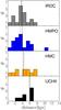 |
Fig. 1 From top to bottom: distance distribution for each of the subsamples, IRDCs, HMPOs, HMCs, and UCHii regions. The bins have widths of 1 kpc and show the number of sources per distance range. The vertical dashed line shows the median distance, the vertical solid line the mean distance of the subsample. |
3. Observations
The 59 sources were observed with the Arizona Radio Observatory Submillimeter Telescope (SMT) in 2013 between February 12−15, March 10−13 and on March 31 and April 1 with ~100 h total observing time. For the observations we used the ALMA type 1.3 mm dual polarization sideband-separating heterodyne receiver and the filterbanks as backends with a resolution of 250 kHz, which corresponds to ~0.3 km s-1 resolution in velocity. The beam size of the SMT at 1.3 mm is ~30″. One single integration took 5 min in position-switching mode, with 2.5 min on-source time. The emission in the deuterated lines was integrated two to three times, the emission in the non-deuterated lines one to two times, depending on the observing conditions. The data was calibrated using data of Jupiter from the same observation runs assuming a sideband rejection of 13 db. The mean system temperatures of the spectra Tsys is 380 K. The data reduction was conducted with the standard GILDAS1 software package CLASS. All spectra from each source were baseline subtracted, calibrated to Tmb scale with typical beam efficiencies of 0.6, and averaged. In a few cases we used the 1 MHz filterbanks spectra because of the very broad lines (e.g., in Orion-KL) or when the line was not detected in the 250 kHz filterbanks (with 128 channels), but in the 1 MHz filterbanks (with 512 channels). The line integrals were measured by summing the line emission channel by channel for detected lines. The detection criteria was a signal-to-noise ratio S/N> 3.
The line parameters of the observed molecules are given in Table 1.
Analyzed molecules with transitions, frequencies, energies of the upper level, and Einstein coefficients Aul.
3.1. Rms
The median 1σ root mean square (rms) values for the deuterated molecules are 0.031 K for DCN (3−2), 0.024 K for DNC (3−2), 0.025 K for DCO+ (3−2), and 0.035 K for N2D+ (3−2). DCN (3−2) was observed in the later shifts, and the higher rms value is due to poorer observing conditions during that period. The higher rms value for N2D+(3−2) is due to problems at this specific transition frequency and is described in the following section. An overview of all rms values is given in Fig. 2. The strong outlier in DCN (3−2) is from Orion-KL, which is still a detection.
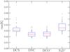 |
Fig. 2 1σ rms values of spectra of the deuterated molecules. The red solid line shows the median, the blue box the 25−75% range, and the crosses mark the outliers. |
3.2. Problems with N2D+ spectra
Reducing and analyzing the spectra of the N2D+ (3−2) transition at 231.32 GHz was problematic because of blending by an overlaying pressure broadened ozone line in the atmosphere. This ozone line depends on the elevation of the source and time of the observation and affects the different sources with varying strength. As a result of this contamination, the mean 1σ rms value of the N2D+ line is 40% higher than for the other deuterated spectral lines, and thus the threshold for a detection is higher. In the five sources IRDC18454.1, IRDC18454.3, Orion-KL, HMC010.47, and HMC031.41 the ozone line prevents distinguishing between a detection or a non-detection.
4. Deuterium fractionation
Under cold conditions, the deuteration fraction of molecules can be enhanced through reactions with, for instance deuterated H , H2D+. While the chemical reaction that deuterates H proceeds without a thermal barrier, the backward reaction is endothermic and has a thermal energy barrier (Watson 1974; Caselli & Ceccarelli 2012; Albertsson et al. 2013). This energy barrier leads to an enhanced formation fraction at low temperatures, but becomes negligible for higher temperatures at which the backward reaction becomes as efficient as the forward reaction. The chemical reactions and their energy barriers that introduce deuterium into some of the key molecules are the following:
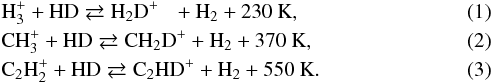 The temperature range for an effective D-enhancement for the pathway via H isotopologs is ~10−30 K, whereas it is ~10−80 K for pathways via light hydrocarbons (Millar et al. 1989; Albertsson et al. 2013). This enhances the deuteration fraction of the key molecules H and CH in different temperature regimes. Another effect that increases the H2D+/H ratio is the depletion of neutral gas-phase species (e.g., CO, N2; see Dalgarno & Lepp 1984; Roberts & Millar 2000). This enhancement is then imprinted on the molecules formed through these reaction partners.
In the literature different models exist that describe the formation routes of deuterated molecules and their relative importance. The dominant formation pathways of DCO+ and N2D+ are via a low-temperature route through H isotopologs, whereas DCN can be formed via a fractionation route involving light hydrocarbons. The back-reaction of the route via H isotopologs sets in at temperatures around 30 K and their deuteration fractions decrease with rising temperature. According to Roueff et al. (2007), both DCN and DNC can be formed efficiently at low temperatures via deuteration of HNC or HCN. However, at higher temperatures DNC is destroyed by reactions with atomic oxygen, unlike DCN. The chemical models of Turner (2001) indicate that only DCN is also formed via reactions with light hydrocarbons involved, but not DNC. If the Turner (2001) scheme is correct, then molecules such as C2D, HDCO or C3HD should show a similar behavior as DCN with temperature, since they are also formed via CH2D+ and C2HD+.
Parise et al. (2009) found a low DCO+/HCO+ column density ratio but significant deuteration fractions for HCN and H2CO under temperature conditions of ~70 K toward the Orion Bar. Model calculations by Roueff et al. (2007) predicted that in general the DNC/HNC, DCO+/HCO+ and N2D+/N2H+ column density ratios decrease with temperature, but are almost constant with density. The DCN/HCN column density ratio shows a more complex behavior with temperature, reaching the highest ratio for ~30 K and shows a stronger increase with density. They found that the reason for this behavior is twofold. First, it is due to the enhanced abundance of radicals (e.g., CHD and CD2) that form DCN. Second, the main destruction pathways of DCN are reactions with the ions HCO+ and H3O+, which leads to DCNH+ which subsequently returns to DCN via dissociative recombination. The deuteration fractions also strongly depend on the assumed elemental abundances.
5. Results
5.1. Detection fractions for DCN, DNC, DCO+, and N2D+
The detection fractions of DCN, DNC, DCO+, and N2D+ in the respective stages are shown in Fig. 3. In this figure, the IRDC stage is split into the two source categories mentioned in Sect. 2, without and with an embedded point source. Based on this figure, we identify three trends:
1) N2D+(3−2) is only detected toward IRDCs and HMPOs. Since the N2H+ abundance is almost constant over the full evolutionary sequence (Paper I), a strong temperature dependence of the N2D+ production leading to its disappearance at T ≳ 30 K is most likely the answer to its apparent absence in the HMC and UCHii stages. Another complication are the problems with the particular bandpass of its (3−2) transition mentioned in Sect. 3.2, which lead to a higher mean 1σ rms value. This does not mean that N2D+ is absent, since some of our sources with non-detections in N2D+(3−2) were detected by Fontani et al. (2011) in N2D+(2−1). This could indicate the importance of excitation conditions for the detection of the (3–2) transitions. Nonetheless, the detection rates of N2D+(3−2) are clearly lower than the detection rates of the other observed molecular transitions of this work. 2) The only deuterated molecule detected in the presumably coldest IRDCs without an embedded point source at 24 μm (Spitzer/MIPSGAL) or 70 μm (Herschel/PACS) is DCO+, which also has the highest detection fraction in the more evolved IRDCs. 3) The detection fractions of DCN, DNC, and DCO+ in warm IRDCs up to UCHii regions are comparable and peak at the HMC stage. In general, the detection fractions toward the observed high-mass star-forming regions are high, ≳60%. It is important to mention here that the strength of a transition is the product of column density and temperature, and thus detections at the lower temperatures present in the earlier stages are more difficult. A lower detection fraction does not necessarily mean that the column densities in the earlier stages are lower than at the later stages. The differences in column densities during the evolutionary sequence are discussed in Sect. 6.1.
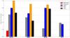 |
Fig. 3 Detection fraction of the four observed deuterated species in the different evolutionary stages. Here the infrared dark cloud (IRDC) stage is divided into the two subsamples without and with an embedded point source at 24 or 70 μm, indicated in the caption as IRDC(wops) and IRDC(wps). The detection fractions are shown from left to right with infrared dark clouds without embedded point sources in red (IRDC(wops)), infrared dark clouds with embedded point sources (IRDC(wps)) in gray, high-mass protostellar objects (HMPO) in blue, hot molecular cores (HMC) in yellow and ultracompact Hii regions (UCHii) in black. |
5.2. Excitation temperatures and final column densities
In this section we discuss the excitation temperatures used to derive the column densities and how we combined the data from Paper I and this work to obtain the final column densities. The column densities are derived in Appendix A.1.
The column densities for the non-deuterated species were partly taken from Gerner et al. (2014) and partly calculated from the new observations. A detailed overview of the exact combination of the previous work and this one is given below. In the previous study we observed the (1−0)-transitions of several molecules with the IRAM 30 m telescope. The size of the beam for these observed (1−0)-transitions is very close to the size of the beam of the (3−2)-transitions observed for this work with the SMT. In the previous work we used likely optically thin (1−0)-transitions of H13CO+ and HN13C and, because of their hyperfine structure, optical-depth-corrected N2H+ and HCN to derive their column densities. The spectra of the first study were partly affected by source emission at the present off-positions and strong optical depth effects. In these cases the optical depth and the integrated intensity could not be reliably determined. Thus we refrained from using these lines in the analysis. In this work we have additional information from the (3−2) transitions to complement the missing column densities. To obtain consistent results from both observation runs we compared the column densities of H13CO+(1−0) with the column densities of H13CO+(3−2) derived with Tex = 20.9 K (IRDC), Tex = 29.5 K (HMPO), Tex = 40.2 K (HMC) and Tex = 36.0 K (UCH ii). These are the mean temperatures of the best-fit models from Gerner et al. (2014). The comparison is shown in Fig. 4.
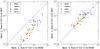 |
Fig. 4 Left: comparison of column densities of H13CO+(1−0) and H13CO+(3−2) assuming the same excitation temperatures for both transitions. Right: comparison of column densities of H13CO+(1−0) and H13CO+(3−2) using the excitation temperatures discussed in Sect. 5.2. The errors show the uncertainties in the measured integrated flux. In some cases that uncertainty is too small to be seen in this plot. |
The derived column densities for the IRAM data are all clearly higher. Excluding problems in the quality of the data and the calibration leads to the assumption that, while the (1−0) transitions are in local thermodynamical equilibrium (LTE), the upper levels are subthermally populated and thus the (3−2) transitions are not in local thermodynamical equilibrium (LTE). This implies that the average densities of the gas are below ~106−107 cm-3. Since the two different lines trace gas with different excitation conditions, the spatial extent probed by the two transitions might be different. However, we do not know the beam-filling factors for the different molecules and their different transitions. In addition, we calculated the column densities from the H13CO+(1−0) and (3−2) transitions with the non-LTE radiative transfer code RADEX2 (van der Tak et al. 2007). The derived column densities for H13CO+ agreed within a factor of 2 with the column densities derived under the assumption of LTE from the H13CO+(1−0) transition. This is well within the uncertainties and validates the assumptions made for the (1−0) transitions. To compensate for the differences in the excitation conditions between (1−0) and (3−2) transitions, we calculated the excitation temperature of the (3−2) transition for each source, which would be necessary to derive the total column densities derived from the (1−0) transition. From those excitation temperatures we computed the median value for each stage. This resulted in Tex = 5.2 (IRDC), Tex = 6.2 (HMPO), Tex = 7.2 (HMC) and Tex = 6.4 (UCH ii) for the (3−2) transitions. The comparison of the calibrated H13CO+(3−2) column densities derived with the lower excitation temperatures and the (1−0) data is shown in Fig. 4. This correction should also reduce the error in the beam-filling fraction and make the different transitions comparable.
For the four different molecules we derived the column densities as described below.
5.2.1. HCO+ and HNC
For HCO+ and HNC we used H13CO+(1−0) and HN13C transitions, assuming the relative isotopic ratio depending on the galactocentric distance described in Wilson & Rood (1994). In Gerner et al. (2014) we used the representative value for the Sun and the local ISM of 12C/13C = 89 (Lodders 2003). This decreases the derived column densities for this work.
5.2.2. N2H+ and HCN
For N2H+ we took the column densities from the (1−0) transitions from Gerner et al. (2014), for which we used, in case of optically thick lines, the optical depth and the excitation temperature from the hyperfine fits made with CLASS3. The hyperfine structure fitting routine (METHOD HFS) assumes that all components of the hyperfine structure have the same excitation temperature and the same width and that the components are separated in frequency by the laboratory values. From the comparison of the ratios of the line intensities of the hyperfine components to the theoretically expected ratios, the fit routine estimates the optical depth of the line. In the optically thick case, this allows us to determine the excitation temperature. In the optically thin case we assumed the excitation temperatures given in Sect. 5.2.
For HCN we used the optical-depth-corrected column densities from the (1−0) transitions when available. In all other cases we computed the mean difference between column densities derived from the (1−0) transitions and the (3−2) transitions and applied this factor of ~1.7 to the derived column densities from the (3−2) transitions.
All column densities are beam-averaged quantities. The resulting median abundances including all detections and upper limits for each subsequent evolutionary phase are given in Table 2. In deriving the column densities, we assumed the excitation temperatures of the deuterated and non-deuterated molecule of the same transition to be equal. This assumption is valid for high densities and high excitation temperatures, but might lead to an underestimation of the deuteration column density ratios Dfrac by a factor of ~2−4 (Shirley, in prep.).
Observed median column densities (N) and the standard deviation (SD) for IRDCs, HMPOs, HMCs, and UCHii regions as a(x) = a × 10x.
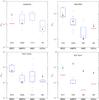 |
Fig. 5 Spread in deuteration fractions Dfrac in the four evolutionary stages for HCN, HNC, HCO+, and N2H+. If there are six or more detections within one stage, the blue box shows the 25−75% range and the crosses mark the other 50% of the data points. If there are fewer than six data points, only the individual data points are shown. The red solid line shows the median of all detections and upper limits. The downward arrow shows the highest value of all upper limits within that stage. The fractions at the bottom of each stage give the detection rate. |
6. Discussion
6.1. Deuteration fractions
The spread of the deuteration fractions Dfrac and the median value for each stage is shown in Fig. 5. These values include detections and upper limits. For N2D+ the median 3σ-limits of non-detections for the HMC-stage and UCHii-stage are given because the detection fraction is zero. These values can be considered as a sensitivity limit.
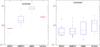 |
Fig. 6 Spread in fractions in the four evolutionary stages for DCN/DNC and HCN/HNC for detections in both molecules only. If there are six or more detections within one stage, the blue box shows the 25−75% range and the crosses mark the other 50% of the data points. If there are fewer than six data points, only the individual data points are shown. The red solid line shows the median of the ratio of detections in both molecules. |
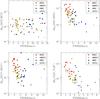 |
Fig. 7 Deuteration fractions of HCN, HNC, HCO+, and N2H+ vs. FWHM of non-deuterated species from HCN (or H13CN in case HCN is not available), HN13C, H13CO+ and N2H+, respectively. The dots mark detections, the triangles upper limits. The typical size of an error bar from the uncertainty in the integrated flux is given in the lower right. |
The ratios of the column densities of DNC, DCO+, and N2D+ with their non-deuterated counterparts HNC, HCO+, and N2H+ all show decreasing trends with evolutionary stage, despite the wide spread of ratios within individual stages. Only HCN shows an increase in the ratio with the maximum reached in the HMC-stage. In some cases the consecutive stages appear not very different from each other within the error budget (e.g., HMPO-HMC of DCO+/HCO+, HMC-UCHii of DNC/HNC). The reason for this is probably that the evolution throughout the sequence is continuous, and there might be overlaps between consecutive stages, for example, some of the HMCs are associated with UCHii regions. One can distinguish between two different scenarios that can lead to an overlap between consecutive stages. For HMC029.96 (G29.96), for instance high spatial resolution observations show a separation of the actual UCHii region and the neighboring HMC of 2″ (Cesaroni et al. 1994; Beuther et al. 2007b). The HMC and the UCHii region are two (or more) distinct entities. The second scenario are cases like HMC009.62 (G9.62), where a separate UCHii region exists as well, but in addition, a small hypercompact Hii region is present at the location of the HMC itself (Testi et al. 2000). This is a general caveat in single-dish observations of HMCs that might be contaminated by UCHii regions in the beam. Here, the sources were classified based on their chemistry which is probably dominated by the HMC. However, this does not totally cancel this effect out, and differences in the measured ratios between different stages are weaker in some cases. Nevertheless, the global trends are clearly visible.
Furthermore, Fig. 6 shows the observed column density ratios of DCN/DNC and HCN/HNC for sources detected in both molecules. While the ratio of the non-deuterated molecules is almost constant, the ratio of the deuterated molecules clearly shows a peak at the HMC stage. reflected by the results of the one-way ANOVA tests that yield probability values p< 10-4 for DCN/DNC and p = 0.17 for HCN/HNC. The KS2 test of the consecutive stages confirms these findings. We conclude that DCN can be formed more efficiently or is destroyed less efficiently than DNC in the more evolved and thus warmer sources. The observed behavior can be understood according to the dominant formation pathways scenario stated by Turner (2001). He claimed that all four deuterated molecules can be efficiently formed at low temperatures via H2D+, but only DCN can be formed at higher temperature via CH2D+. This would lead to the observed trends in the deuteration fractions, since DCN can still be formed in the more evolved stages, in contrast to the other observed deuterated molecules. However, newer chemical models (e.g., Roueff et al. 2007) or the updated model we use, do not support this scenario of a difference in dominant formation pathways between DCN and DNC. According to these new models, both isomers are formed from light hydrocarbons and thus exhibit a similar evolution in the abundance ratios with temperature. Hiraoka et al. (2006) studied the association reactions of CN with D in laboratory experiments and found an intensity ratio of DNC/DCN of ~3 at a temperature of 10 K. At temperatures >20 K, the formation of DNC and DCN became negligible. This is consistent with the derived value for the IRDC stage in this work on the order of unity, but contradicts the higher DCN/DNC ratios found in the HMC stage, suggesting another possible formation route. The HCN/HNC median ratios is between 0.4−1.4 in the different stages and slightly increases with stage. This is consistent within the observational uncertainties with theoretical expectations of the ratio of 1 in cold clouds and >1 in warmer clouds (Sarrasin et al. 2010).
6.2. Relation between deuteration and other parameters
We measured the full width at half maximum (FWHM) of HCN, HN13C, H13CO+ and N2H+. The isotopologs were assumed to be optically thin. For N2H+ and HCN we corrected the measured optically thick FWHM Δνthick according to Phillips et al. (1979) using the relation
 (4)where τ is the optical depth of the line center and FWHMthin the optically thin FWHM. We tested for linear relationships using the Pearson correlation coefficient. By definition, the absolute value of ρ is ≤1 with a stronger correlation for larger ρ. ρ = 0 means no correlation. The sign indicates a positive or negative correlation between the two quantities. To estimate ρ we randomly drew sets of data points from the measured values with their corresponding errors and the upper limits, and found for each of these drawn data sets the underlying correlation coefficient. We then determined the most frequent correlation coefficient among all data sets and its 16% and 84% confidence values (Bailer-Jones et al., in prep.). The correlation plots are shown in Fig. 7, and the corresponding Pearson correlation coefficients ρ are given in Table 3. The plots show that earlier phases have a smaller FWHM.
Correlation coefficients ρ with 16% and 84% confidence values.
The resulting coefficient is consistent with the data being uncorrelated for all four molecules. The FWHM of N2H+ might be an exception and correlated, but is still <0.5 and no conclusive answer can be given. Although the correlation with the FWHM is weak, the decrease of the deuterium ratio with increasing FWHM is consistent with the picture of more quiescent, early stages with lower FWHM and higher deuteration fractions followed by more turbulent stages with higher FWHM and lower deuterium ratios.
Furthermore, we studied the correlation of the deuteration with the H2 column density and luminosity L. The luminosities and H2 column densities are shown in Tables A.2–A.3 and the corresponding correlation plots in Figs. 8 and 9. In general, the deuteration fraction shows similarly weak correlations with the luminosities as with the FWHM. Clearly, there is a lack of correlation with H2 column densities. Of the four deuteration fractions, the strongest correlation is found for N2D+, but the correlation is still very low. The luminosity of a source is not necessarily a tracer of its evolutionary stage, but Fig. 8 shows that the four different evolutionary stages are approximately separated with respect to the luminosity. Taking into account that the temperature of the objects increases with evolutionary stage, the luminosity can be used as a proxy for the temperature in the case of our source sample. Since higher luminosities indicate higher temperatures and smaller regions with T ≲ 20 K, where CO is frozen out, it reduces the overall abundance as well as the D/H ratio of N2H+. Of all four molecular deuteration fractions, DCN and DCO+ show the weakest correlation with any of the shown parameters. However, none of the studied correlations have correlation coefficients ρ> 0.5.
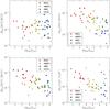 |
Fig. 8 Deuteration fractions of HCN, HNC, HCO+ and N2H+ vs. the luminosity of the source. The dots mark detections, the triangles upper limits. The typical size of an error bar from the uncertainty in the integrated flux is given in the lower right. |
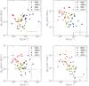 |
Fig. 9 Deuteration fractions of HCN, HNC, HCO+, and N2H+ vs. the H2 column density of the source. The typical size of an error bar from the uncertainty in the integrated flux and from the uncertainty in the derived H2 column densities (see Sect. A.1) is given in the lower right corner. |
6.3. Modeling the chemical evolution
With the observed column densities of 18 species (14 from Paper I) including 4 deuterated species in different stages of massive star formation at hand, we applied the iterative physico-chemical fitting model MUlti Stage CLoud codE with D-chemistry (MUSCLE-D) to these data. A list of all fitted species is given in Table 4. The model fits the evolution of the observed chemical data and thereby constrains basic physical properties in the assumed evolutionary path of high-mass star formation, such as mean temperatures and mean chemical ages. The chemical ages can be interpreted as typical lifetimes of the various stages. This model is the extended version of the iterative fitting model MUlti Stage CLoud codE (MUSCLE) already used and described in Gerner et al. (2014) and includes a physical and a chemical model. Here we briefly summarize the main characteristics of the two parts of MUSCLE-D, the physical model in Sect. 6.3.1 and the chemical model ALCHEMIC in Sect. 6.3.2.
Species fitted with the model.
6.3.1. Physical model
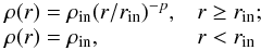
The physical model treats the star-forming region as spherically symmetric 1D-clouds with a fixed outer radius of rout = 0.5 pc, based on the largest beam size of our observations of 30″ and the typical size of high-mass star-forming regions. High angular resolution studies revealed in some of the sources complex structures that deviate from the spherically symmetric case (e.g., Beuther et al. 2002a). However, in single-dish maps these sources appear to be symmetric (e.g., Beuther et al. 2002b). Since we analyzed single-dish data, a 1D physical model appears to be sufficient. More sophisticated models that take into account complicated substructures would increase the number of fitting parameters and might lead to an overinterpretation of the data. The radial density and temperature structure is modeled with
 (5)and
 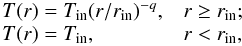 (6)respectively. The temperature and density profiles do not change with time. The fitted physical quantities are the inner radius rin, the temperature and density at the inner radius, Tin and ρin and the power-law index of the density p. The inner radius is limited between 5 × 10⁻⁵−5 × 10⁻² pc. While we modeled the IRDC as an isothermal sphere, the temperature structure of the more evolved stages is modeled by a inner flat plateau with Tin and a power law with slope q = 0.4 as a standard value for r>rin (see van der Tak et al. 2000). The radial density profile within rin is flat with ρin and decreases for r>rin as a power law with slope p. The value of p was limited to values between 1.5 and 2.0 to save computing time. This range is supported by several observations, for example, Guertler et al. (1991), Beuther et al. (2002b), Mueller et al. (2002), and Hatchell & van der Tak (2003). The temperature and density profiles were fitted simultaneously. The model does not take into account radiative transport. In the model, the whole cloud is embedded in a larger diffuse low-density medium that shields the high-mass star-forming cloud from the interstellar FUV radiation.
6.3.2. Chemical model
The chemical model is an updated version of the time-dependent gas-grain chemical model ALCHEMIC described in Semenov et al. (2010) that we used and described in Gerner et al. (2014). In addition to this, the deuterium network from Albertsson et al. (2013) was added and extended with high-temperature reactions (Harada et al. 2010, 2012; Albertsson et al. 2014b) and ortho/para states of H2, H and H and their isotopologs (Albertsson et al. 2014a). In total, the chemical network comprises 15 elements that can form 1260 different species from 38 500 reactions.
The initial abundances prior to the IRDC stage are taken from the low-metals set given in Lee et al. (1998) with a changed elemental abundance of Si (3 × 10⁻⁹ with respect to H) and S (8 × 10⁻⁷ with respect to H). The changes were needed to achieve proper fits to the IRDC phase. Initially, all metals (C, O, N, S, etc.) are in atomic form. Only H2 is already in molecular form. The initial ortho-para ratio of H2 is assumed to be the statistical value of 3:1. The model includes nuclear spin-state exchange reactions to account for the evolution of the ortho-para ratio and freeze out of CO. For the subsequent stages, the chemical outcome of the previous best-fit model is used as input initial abundances.
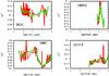 |
Fig. 10 Evolution of the minimum χ2 of the best-fit models with time. The four panels show the four different stages IRDC (upper left), HMPO (upper right), HMC (lower left), and UCHii (lower right). The red curve marks the calculated values at all 299 time moments, the green curve shows their smoothed spline interpolation. |
6.3.3. Fitting procedure
The different stages were fit iteratively using the physical and chemical model described above. We modeled the observed column densities for the IRDC, HMPO, and HMC stage by varying the parameters rin, Tin, ρin and p. While keeping all other parameters fixed, we varied these four parameters and ran the model over 105 yr for each of the realizations. Then we computed the χ2-value for each time step and model realization, given the observed mean column densities and computed model column densities. We assumed the standard deviation between modeled and observed values to be one order of magnitude as a typical value. Molecules that were detected in less than 50% of the sources within one stage were considered as upper limits. Finally, the model with the minimum χ2-value was found as the best-fit model that matches with the calculated mean column densities for each stage best.
As a result of the iterative fitting along the evolutionary sequence, the introduced uncertainties increase with evolutionary stage, leading to a limited confidence in the obtained results for the later stages.
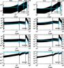 |
Fig. 11 Modeled and observed relative abundances to H2 are plotted for the IRDC-UCHii stages. The modeled values are shown by the black solid line, the observed values show the median of all detections and upper limits, and are depicted by the blue dashed line. The error bars are indicated by the vertical marks. |
6.4. Modeling results
We fitted the combined data from Gerner et al. (2014) and this work with this model assuming an ortho-para H2 ratio o/p = 3:1. The resulting best-fit model parameters for the IRDC, HMPO, HMC, and UCHii stage are shown in Tables A.4−A.7. The evolution of the best-fits with time is shown in Fig. 10. These distributions give a good impression of the uncertainty on the chemical age. The best-fit lifetime is 16 500 yr for the IRDC stage. A good fit was also achieved with a chemical age of only 1000 yr. However, this seems to be a rather short time and might be interpreted as a lower limit. The HMPO best-fit age yielded 32 000 yr with probable values between 10 000−40 000 yr. For the HMC stage we found a best-fit age of 35 000 yr; values below 15 000 yr are improbable. The best-fit age for the UCHii stage was found to be rather young with 3000 yr, but quite unconstrained with probable values up to several 10 000 yr.
The observed and modeled column densities are shown in Tables A.8−A.11. The best-fit of the IRDC stage reproduces 18 of 18 molecules within the assumed combined (observational + chemical) uncertainty of one order of magnitude. In the HMPO stage the model is able to reproduce 16 of 18 molecules. SO is overproduced by a factor of ~20 and CH3OH underproduced by a factor of ~40. The underproduction of methanol is possibly due to shock- or outflow-triggered enhanced desorption of methanol ice from grains, which is not taken into account in the model. The reason for the misfit of SO might be the poorly understood chemistry of sulfur-bearing species in modern astrochemical models in general. In the HMC stage the model could fit 14 of 18 species. In addition to C2H, which is ~20 times underproduced, HNCO, SO, and CH3OH are misfit by more than a factor of 100. The underproduction of CH3OH and overproduction of SO in the HMPO stage continues in the HMC phase. The overproduction of HNCO might be connected to not well enough understood shock- and surface chemistry. This difference in C2H between the model and observations might be influenced by UV-radiation of the central star(s) or a clumpy structure of the environment, which is not considered in the model. This is especially important for the UCHii regions, but it is also already present in some HMCs. For the last considered stage of an UCHii region, the model reproduces 13 of 18 species. As in the HMC stage, the molecules HNCO, SO, and C2H are misfitted in the UCHii stage. In addition, SiO and DCO+ are slightly overproduced.
In general, the overall fit of all 18 molecules of the four fitted phases is good. The specific time dependent evolution of the best-fit abundances of molecules DCN, DNC, DCO+, N2D+ and their non-deuterated counterparts are shown in Fig. 11. Between two consecutive stages, the physical parameters are instantly changed and the molecular species show a quick response to that change, followed by a slower evolution under the new constant conditions. Figures A.1–A.4 show the modeled column densities in each stage separately. In total, the best-fit ages add up to 85 000 yr, which is on the same order as typical models of high-mass star formation of 105 yr (e.g., McKee & Tan 2003; Tan et al. 2014).
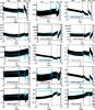 |
Fig. 12 Modeled and observed column density ratios are plotted for all stages. The modeled values are shown by the black solid line, the observed values show the median of all detections and upper limits, and are depicted by the blue dashed line. The error bars are indicated by the vertical marks. |
The evolution for the different molecular ratios are shown in Fig. 12. The modeled abundance ratios partly show larger deviations from the observed values because the uncertainties from both molecules add up. In Sect. 6.1 we discussed the ratio of DCN/DNC and a possible chemical explanation based on a chemical network by Turner (2001). However, the chemical network used in our work shows a different trend with a constant ratio rather than an increase of DCN/DNC with temperature. Thus the observed trend disagrees with our model predictions, and the possibility of different chemical formation pathways needs to be tested by future observations of more deuterated molecules sharing the same formation pathways as DCN (e.g., light hydrocarbons with two or three C-atoms). The model agrees with the constant ratio of HNC/HCN of unity with recent developments in the collisional rates by Sarrasin et al. (2010).
6.5. Comparison with best-fit models of Paper I
In Paper I we iteratively fitted our model to an observational dataset containing the median column densities of 14 different non-deuterated species. The column densities were derived with typical temperatures for each stage. The model followed the observed evolution and successfully fit most of the species with few exceptions in individual stages. The fits also constrained the physical structure of the model and yielded mean best-fit temperatures for each stage. The mean temperatures deviated from the temperatures used to derive the observed column densities for the later stages. In a second step we fitted the newly derived column densities. The temperature in the best-fit models decreased again and we could not find a converging solution.
In this work we used the best-fit temperatures of the first model from Paper I to recalculate the median column densities for the previously analyzed 14 species and an additional four deuterated species. The temperature in the best-fit model of the IRDC stage is lower by a factor of 2 compared to Paper I, but the best-fit temperatures of the IRDC stage for both Paper I and this work agree with typical IRDC temperatures. The mean density increased by about an order of magnitude. The best-fit lifetime in this work is a factor of 1.5 longer, but agrees within the assumed uncertainties. The HMPO best-fit mean temperature in this work is lower by 30%. The mean density increased by a factor 3−4. The best-fit lifetime is shorter by a factor of ~2. The HMC best-fit mean temperature in this work is higher by 25%. The mean densities are similar. In comparison to Paper I, the best-fit lifetime is about 20% lower. The UCHii best-fit mean temperatures are similar. The best-fit ages deviate by a factor of 4, but are consistent within their likely ranges. The mean density is lower by one order of magnitude.
The total lifetimes from the IRDC to the UCHii phase in Paper I add up to ~110 000 yr. This work yields a total lifetime that is slightly shorter with ~85 000 yr. The molecules that could not be reproduced in Paper I and this work are not the same. Possible reasons are the additional four deuterated molecules as free fit parameters that were treated with equal weight as well as the revised excitation temperatures used to derive column densities compared to Paper I (see Sect. 5.2). Although D-chemistry is seen as a tracer of the thermal history and conditions of an object and we see weak correlations with luminosity as an evolutionary tracer, the model fits did not improve substantially. Increasing the number of fitted molecules from 14 to 18 species did not improve the achieved results much, probably because the less statistical importance of the deuterated molecules within the total number of 18 species.
6.6. Comparison with literature
In low-mass star formation both observations and theory show that it is possible to use the deuteration fraction of a molecule as an evolutionary tracer (e.g., Crapsi et al. 2005; Aikawa et al. 2005; Emprechtinger et al. 2009). In a recent work, Fontani et al. (2011) observed 27 cores within high-mass star-forming regions and derived the deuteration fraction of N2D+/N2H+. They found a similar behavior as in the low-mass regime. The deuteration fraction is highest in the starless cores with Dfrac = 0.26 and decreases during the formation of the protostellar objects to Dfrac = 0.04. We find a similar trend in our work, but the median deuteration fraction we measure in our IRDC sample is lower by a factor of four than their high-mass starless core sample. This might be due to the fact that our IRDC sample contains starless as well as already more evolved objects inhabiting 24 μm sources. The same is true for the HMPO samples of Fontani et al. (2011) and this work. We find lower ratios by about a factor of four. The highest D/H ratio is that of N2D+/N2H+ in IRDC20081 of Dfrac = 0.12. This source inhabits no point sources below 70 μm, but it is close to a nearby source with extended emission. It is presumably in a very early pre-stellar phase. Miettinen et al. (2011) studied seven massive clumps within IRDCs and derived deuteration fractions for N2H+ between 0.002−0.028 and for HCO+ between 0.0002−0.014. While the range of values for HCO+ is comparable with the IRDCs in our sample, the deuteration fractions for N2H+ are about one order of magnitude higher in this work. However, this agrees with the high number of upper limits due to non-detections of N2D+ in this work. Chen et al. (2011) observed several cores in various evolutionary stages and found deuteration values of N2H+ between 0.004−0.1. The source lists have three targets in common. For the HMPO18151 both works agree on a value of Dfrac = 0.01. For the other two sources in common, IRDC18151 and IRDC18223, we find a slightly higher value of Dfrac = 0.03 instead of Dfrac = 0.02. While the highest value they found is similar to the highest value we observe, they detected N2D+ in more sources and also found lower deuteration fractions, especially in the more evolved sources for which we have no detections of N2D+. Crapsi et al. (2005) studyied the N2D+/N2H+ ratio in low-mass starless cores and revealed deuteration fractions on the percentage level up to almost 50% in the most extreme case of Oph D. The highest ratio observed in our survey is ~0.1. Sakai et al. (2012) measured deuteration fractions of DNC/HNC for IRDCs and HMPOs. They found Dfrac = 0.003−0.03 for Midcourse Space Experiment (MSX) dark sources at 8 μm and Dfrac = 0.005−0.01 for HMPOs. These ratios agree well with Dfrac = 0.004−0.02 for our IRDC sample and Dfrac = 0.0015−0.015 for our HMPO sample. In a recent study, Kong et al. (2013) explored the effect of different parameters on the deuteration fraction of N2H+ in dense and cold environments. They found an increase of the deuteration fraction with decreasing temperature. However, they also found a positive correlation with the density, which is not clearly seen in our data. They employed a 0D model to study deuteration in star-forming clouds and found that the timescales to reach equilibrium in the abundances is on the order of several free-fall times (~106 yr) for typical densities of high-mass cores. In contrast, the best-fit models in our work are not supposed to reach chemical equilibrium and thus our model predicts a total timescale of ~105 yr for the best-fit models. This is probably because in a 1D model with a power-law density profile with higher densities in the inner region timescales in the chemical evolution are shorter than in a 0D model.
7. Conclusion
We extended the analysis from Gerner et al. (2014) of the chemical evolution in 59 high-mass star-forming regions for deuterated molecules. We measured beam averaged column densities and deuteration fractions of the four deuterated species DCO+, DCN, DNC, and N2H+. We found an overall high detection fraction toward the high-mass star-forming regions, except for N2D+, which is probably due to the limited sensitivity of our survey. The detection fraction of DCO+, DCN, and DNC increases from IRDCs to HMPOs and peaks at the HMC sample, where we detect all three molecules in all sources but one, and it drops again toward the UCHii stage.
The (3−2) lines are subthermally populated. The median deuteration fractions excluding upper limits are 0.02 for DCN, 0.005 for DNC, 0.0025 for DCO+, and 0.02 for N2D+. The deuteration fractions of DNC, DCO+, and N2D+ show a decreasing trend from IRDCs over HMPOs and HMCs to UCHii regions, which supports the hypothesis that deuterated molecules may be used as indicators of the evolutionary stage in high-mass star-forming regions.
In general, we find no correlation between the deuteration fraction of the various molecules and physical parameters for DCO+/HCO+ and DCN/DNC. Only N2D+/N2H+ shows a slight anticorrelation with the luminosity and the FWHM. The total measured column density of the gas does not correlate with the deuteration fraction. This result indicates that within the range of probed densities, deuteration depends more strongly on the temperature of the environment than on the column density and is enhanced in colder, less luminous regions. However, Albertsson et al. (2013), for example, found in their models differences in the deuteration with density at lower densities.
The slight anticorrelation with luminosity and FWHM, which is related to the evolutionary stage, indicates that evolutionary stage plays an important role for the deuteration fraction. But its huge scatter within single stages leads to the assumption that the evolution might not be the only factor.
Furthermore, we fit the observed data with a chemical model and find reasonable physical model fits. Combining observations of non-deuterated and deuterated species to obtain best-fits led to reasonable chemical and physical models. The best-fit models produce reasonably good results for all stages. As a result of the large uncertainties in the observations and the model and the wide spread of observed values within the four subsamples, we could not substantially improve the best-fit model results compared to Paper I. Another reason is that the combination of the four deuterated molecules with the 14 non-deuterated species probably reduced the statistical importance of each molecule and thus the effect on the best-fit of the model.
Online material
Appendix A
Appendix A.1: Molecular column densities
We calculated the molecular column densities of the upper level of a particular transition following the equation for optically thin emission ![Mathematical equation: \appendix \setcounter{section}{1} \begin{equation} N_{\rm u}=\frac{8 \pi k \nu^2}{h c^3 A_{\rm ul}} \frac{J_{\nu}(T_{\rm ex})}{[J_{\nu}(T_{\rm ex})-J_{\nu}(T_{\rm cmb})]} \cdot \int T_{\rm mb} \delta \nu, \end{equation}](/articles/aa/full_html/2015/07/aa23989-14/aa23989-14-eq155.png) (A.1)where the integrated intensity given in K km s-1, and the Einstein coefficient Aul is in s-1, and with
(A.1)where the integrated intensity given in K km s-1, and the Einstein coefficient Aul is in s-1, and with ![Mathematical equation: \appendix \setcounter{section}{1} \begin{equation} J_{\nu}(T)=\frac{h \nu /k }{\exp[h \nu/k T] - 1} , \end{equation}](/articles/aa/full_html/2015/07/aa23989-14/aa23989-14-eq156.png) (A.2)where ν is the frequency of the observed transition (e.g., Mangum & Shirley 2015). Then the total column density (which we refer to from now on as column density) can be calculated:
(A.2)where ν is the frequency of the observed transition (e.g., Mangum & Shirley 2015). Then the total column density (which we refer to from now on as column density) can be calculated: ![Mathematical equation: \appendix \setcounter{section}{1} \begin{equation} N_{\rm tot} = N_{\rm u} \cdot \frac{Q}{g_{\rm u} \exp[-E_{\rm u}/kT_{\rm ex}]} \cdot \end{equation}](/articles/aa/full_html/2015/07/aa23989-14/aa23989-14-eq158.png) (A.3)When we were able derive the optical depth τ from hyperfine splitting, we corrected for the column density using
(A.3)When we were able derive the optical depth τ from hyperfine splitting, we corrected for the column density using ![Mathematical equation: \appendix \setcounter{section}{1} \begin{equation} N_{\rm corr} = N_{\rm tot} \cdot \frac{\tau}{1 - \exp[-\tau]}\cdot \end{equation}](/articles/aa/full_html/2015/07/aa23989-14/aa23989-14-eq159.png) (A.4)
(A.4)
To obtain abundances, we derived H2 column densities either from dust maps obtained with Mambo with the IRAM 30 m telescope at 1.2 mm (Beuther et al. 2002b) which provides a resolution of 11″, or the galactic plane survey ATLASGAL (Schuller et al. 2009) at 870 μm with a resolution of 19.2″, or the SCUBA Legacy Catalog (Di Francesco et al. 2008) at 850 μm with a resolution of 22.9″ (see Table A.1). The continuum data were smoothed to 29″ resolution to be beam-matched with the IRAM 30 m observations at 3 mm and the SMT molecular line data. H2 column densities were calculated from the observed peak intensities assuming optically thin emission and LTE following Eq. (A.5) (Schuller et al. 2009). The dust opacities used were κ850 μm = 1.48, κ870 μm = 1.42, κ1.2 mm = 0.97, interpolated values from Ossenkopf & Henning (1994), assuming grains with thin ice mantles, gas densities of n = 105 cm-3, and a gas-to-dust mass ratio R = 100. With these assumptions the H2 column density is calculated as 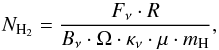 (A.5)The uncertainties in the derived H2 column densities are mainly based on the dust and temperature properties and are about a factor of 3. A more detailed description of the derivation is given in Gerner et al. (2014).
The molecular column densities are then divided by the H2 column densities, and the averaged abundances are derived.
Source list showing the position, the distance, and the evolutionary stage of all high-mass star-forming regions.
Luminosity, H2, DCO+, DCN, DNC, and N2D+ column density and the corresponding error (Δ) for each source.
HCO+, HCN, HNC, and N2H+ column density and corresponding error (Δ) for each source.
Parameters of the best-fit IRDC model.
Parameters of the best-fit HMPO model.
Parameters of the best-fit HMC model.
Parameters of the best-fit UCHii model.
Median column densities in a(x) = a × 10x for observations (including detections and upper limits) and best-fit IRDC model.
Median column densities in a(x) = a × 10x for observations (including detections and upper limits) and best-fit HMPO model.
Median column densities in a(x) = a × 10x for observations (including detections and upper limits) and best-fit HMC model.
Median column densities in a(x) = a × 10x for observations (including detections and upper limits) and best-fit UCHii model.
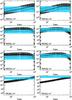 |
Fig. A.1 Observed and modeled column densities in cm-2 at the IRDC stage. The observed values are shown in blue, the modeled values in black. The error bars are indicated by the vertical marks. Molecules are labeled in the plots. |
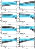 |
Fig. A.2 Observed and modeled column densities in cm-2 at the HMPO stage. The observed values are shown in blue, the modeled values in black. The error bars are indicated by the vertical marks. Molecules are labeled in the plots. |
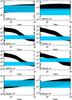 |
Fig. A.3 Observed and modeled column densities in cm-2 at the HMC stage. The observed values are shown in blue, the modeled values in black. The error bars are indicated by the vertical marks. Molecules are labeled in the plots. |
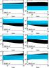 |
Fig. A.4 Observed and modeled column densities in cm-2 at the UCHii stage. The observed values are shown in blue, the modeled values in black. The error bars are indicated by the vertical marks. Molecules are labeled in the plots. |
Acknowledgments
The authors thank the anonymous referee for helping to improve the paper. T.G. is supported by the Sonderforschungsbereich SFB 881 “The Milky Way System” (subproject B3) of the German Research Foundation (DFG). T.G. is member of the IMPRS for Astronomy & Cosmic Physics at the University of Heidelberg. This research made use of NASA’s Astrophysics Data System. D.S. acknowledges support by the Deutsche Forschungsgemeinschaft through SPP 1385: “The first ten million years of the solar system − a planetary materials approach” (SE 1962/1-2 and SE 1962/1-3). TA acknowledges funding from the European Community’s Seventh Framework Programme [FP7/2007-2013] under grant agreement No. 238258. In the reduction and analysis of the data we made use of the GILDAS software public available at http://www.iram.fr/IRAMFR/GILDAS. The SMT and Kitt Peak 12 m are operated by the Arizona Radio Observatory (ARO), Steward Observatory, University of Arizona, with support through the NSF University Radio Observatories program (URO: AST-1140030).
References
- Aikawa, Y., Herbst, E., Roberts, H., & Caselli, P. 2005, ApJ, 620, 330 [NASA ADS] [CrossRef] [Google Scholar]
- Albertsson, T., Semenov, D. A., Vasyunin, A. I., Henning, T., & Herbst, E. 2013, ApJS, 207, 27 [NASA ADS] [CrossRef] [Google Scholar]
- Albertsson, T., Indriolo, N., Kreckel, H., et al. 2014a, ApJ, 787, 44 [NASA ADS] [CrossRef] [Google Scholar]
- Albertsson, T., Semenov, D., & Henning, T. 2014b, ApJ, 784, 39 [NASA ADS] [CrossRef] [Google Scholar]
- Barnes, P. J., Yonekura, Y., Fukui, Y., et al. 2011, ApJS, 196, 12 [NASA ADS] [CrossRef] [Google Scholar]
- Beuther, H., Schilke, P., Gueth, F., et al. 2002a, A&A, 387, 931 [NASA ADS] [CrossRef] [EDP Sciences] [Google Scholar]
- Beuther, H., Schilke, P., Menten, K. M., et al. 2002b, ApJ, 566, 945 [NASA ADS] [CrossRef] [Google Scholar]
- Beuther, H., Schilke, P., Sridharan, T. K., et al. 2002c, A&A, 383, 892 [NASA ADS] [CrossRef] [EDP Sciences] [Google Scholar]
- Beuther, H., Zhang, Q., Greenhill, L. J., et al. 2004, ApJ, 616, L31 [Google Scholar]
- Beuther, H., Churchwell, E. B., McKee, C. F., & Tan, J. C. 2007a, in Protostars and Planets V, eds. B. Reipurth, D. Jewitt, & K. Keil, 165 [Google Scholar]
- Beuther, H., Zhang, Q., Bergin, E. A., et al. 2007b, A&A, 468, 1045 [NASA ADS] [CrossRef] [EDP Sciences] [Google Scholar]
- Beuther, H., Tackenberg, J., Linz, H., et al. 2012, A&A, 538, A11 [NASA ADS] [CrossRef] [EDP Sciences] [Google Scholar]
- Bourke, T. L., Myers, P. C., Caselli, P., et al. 2012, ApJ, 745, 117 [NASA ADS] [CrossRef] [Google Scholar]
- Campbell, M. F., Butner, H. M., Harvey, P. M., et al. 1995, ApJ, 454, 831 [NASA ADS] [CrossRef] [Google Scholar]
- Carey, S. J., Feldman, P. A., Redman, R. O., et al. 2000, ApJ, 543, L157 [NASA ADS] [CrossRef] [Google Scholar]
- Caselli, P., & Ceccarelli, C. 2012, A&ARv, 20, 56 [NASA ADS] [CrossRef] [MathSciNet] [Google Scholar]
- Caselli, P., Stantcheva, T., Shalabiea, O., Shematovich, V. I., & Herbst, E. 2002, Planet. Space Sci., 50, 1257 [NASA ADS] [CrossRef] [Google Scholar]
- Cesaroni, R., Churchwell, E., Hofner, P., Walmsley, C. M., & Kurtz, S. 1994, A&A, 288, 903 [NASA ADS] [Google Scholar]
- Chen, H.-R., Welch, W. J., Wilner, D. J., & Sutton, E. C. 2006, ApJ, 639, 975 [NASA ADS] [CrossRef] [Google Scholar]
- Chen, H.-R., Liu, S.-Y., Su, Y.-N., & Wang, M.-Y. 2011, ApJ, 743, 196 [NASA ADS] [CrossRef] [Google Scholar]
- Churchwell, E., Walmsley, C. M., & Cesaroni, R. 1990, A&AS, 83, 119 [NASA ADS] [Google Scholar]
- Crapsi, A., Caselli, P., Walmsley, C. M., et al. 2005, ApJ, 619, 379 [Google Scholar]
- Dalgarno, A., & Lepp, S. 1984, ApJ, 287, L47 [NASA ADS] [CrossRef] [Google Scholar]
- Daniel, F., Cernicharo, J., Roueff, E., Gerin, M., & Dubernet, M. L. 2007, ApJ, 667, 980 [NASA ADS] [CrossRef] [Google Scholar]
- Di Francesco, J., Johnstone, D., Kirk, H., MacKenzie, T., & Ledwosinska, E. 2008, ApJS, 175, 277 [NASA ADS] [CrossRef] [Google Scholar]
- Ellsworth-Bowers, T. P., Rosolowsky, E., Glenn, J., et al. 2015, ApJ, 799, 29 [NASA ADS] [CrossRef] [Google Scholar]
- Emprechtinger, M., Caselli, P., Volgenau, N. H., Stutzki, J., & Wiedner, M. C. 2009, A&A, 493, 89 [NASA ADS] [CrossRef] [EDP Sciences] [Google Scholar]
- Fontani, F., Caselli, P., Crapsi, A., et al. 2006, A&A, 460, 709 [NASA ADS] [CrossRef] [EDP Sciences] [Google Scholar]
- Fontani, F., Palau, A., Caselli, P., et al. 2011, A&A, 529, L7 [NASA ADS] [CrossRef] [EDP Sciences] [Google Scholar]
- Friesen, R. K., Kirk, H. M., & Shirley, Y. L. 2013, ApJ, 765, 59 [NASA ADS] [CrossRef] [Google Scholar]
- Gerner, T., Beuther, H., Semenov, D., et al. 2014, A&A, 563, A97 [NASA ADS] [CrossRef] [EDP Sciences] [Google Scholar]
- Guertler, J., Henning, T., Kruegel, E., & Chini, R. 1991, A&A, 252, 801 [NASA ADS] [Google Scholar]
- Harada, N., Herbst, E., & Wakelam, V. 2010, ApJ, 721, 1570 [NASA ADS] [CrossRef] [Google Scholar]
- Harada, N., Herbst, E., & Wakelam, V. 2012, ApJ, 756, 104 [NASA ADS] [CrossRef] [Google Scholar]
- Hatchell, J., & van der Tak, F. F. S. 2003, A&A, 409, 589 [NASA ADS] [CrossRef] [EDP Sciences] [Google Scholar]
- Hatchell, J., Thompson, M. A., Millar, T. J., & MacDonald, G. H. 1998, A&AS, 133, 29 [NASA ADS] [CrossRef] [EDP Sciences] [Google Scholar]
- Heitsch, F., Hartmann, L. W., Slyz, A. D., Devriendt, J. E. G., & Burkert, A. 2008, ApJ, 674, 316 [NASA ADS] [CrossRef] [Google Scholar]
- Hiraoka, K., Ushiama, S., Enoura, T., et al. 2006, ApJ, 643, 917 [NASA ADS] [CrossRef] [Google Scholar]
- Kong, S., Caselli, P., Tan, J. C., & Wakelam, V. 2013, ApJ, submitted [arXiv:1312.0971] [Google Scholar]
- Lee, H.-H., Roueff, E., Pineau des Forets, G., et al. 1998, A&A, 334, 1047 [NASA ADS] [Google Scholar]
- Linsky, J. L. 2003, Space Sci. Rev., 106, 49 [NASA ADS] [CrossRef] [Google Scholar]
- Linz, H., Stecklum, B., Henning, T., Hofner, P., & Brandl, B. 2005, A&A, 429, 903 [NASA ADS] [CrossRef] [EDP Sciences] [Google Scholar]
- Lodders, K. 2003, ApJ, 591, 1220 [NASA ADS] [CrossRef] [Google Scholar]
- Mangum, J. G., & Shirley, Y. L. 2015, PASP, in press [arXiv:1501.01703] [Google Scholar]
- McKee, C. F., & Tan, J. C. 2003, ApJ, 585, 850 [NASA ADS] [CrossRef] [MathSciNet] [Google Scholar]
- Miettinen, O., Hennemann, M., & Linz, H. 2011, A&A, 534, A134 [NASA ADS] [CrossRef] [EDP Sciences] [Google Scholar]
- Millar, T. J., Bennett, A., & Herbst, E. 1989, ApJ, 340, 906 [NASA ADS] [CrossRef] [Google Scholar]
- Mueller, K. E., Shirley, Y. L., Evans, N. J., & Jacobson, H. R. 2002, ApJS, 143, 469 [NASA ADS] [CrossRef] [Google Scholar]
- Müller, H. S. P., Schlöder, F., Stutzki, J., & Winnewisser, G. 2005, J. Mol. Struct. 742, 215 [Google Scholar]
- Narayanan, D., Cox, T. J., Shirley, Y., et al. 2008, ApJ, 684, 996 [NASA ADS] [CrossRef] [Google Scholar]
- Oliveira, C. M., Hébrard, G., Howk, J. C., et al. 2003, ApJ, 587, 235 [NASA ADS] [CrossRef] [Google Scholar]
- Ossenkopf, V., & Henning, T. 1994, A&A, 291, 943 [NASA ADS] [Google Scholar]
- Parise, B., Leurini, S., Schilke, P., et al. 2009, A&A, 508, 737 [NASA ADS] [CrossRef] [EDP Sciences] [Google Scholar]
- Phillips, T. G., Huggins, P. J., Wannier, P. G., & Scoville, N. Z. 1979, ApJ, 231, 720 [NASA ADS] [CrossRef] [Google Scholar]
- Pillai, T., Wyrowski, F., Hatchell, J., Gibb, A. G., & Thompson, M. A. 2007, A&A, 467, 207 [NASA ADS] [CrossRef] [EDP Sciences] [Google Scholar]
- Ragan, S., Henning, T., Krause, O., et al. 2012, A&A, 547, A49 [NASA ADS] [CrossRef] [EDP Sciences] [Google Scholar]
- Roberts, H., & Millar, T. J. 2000, A&A, 361, 388 [NASA ADS] [Google Scholar]
- Roueff, E., Parise, B., & Herbst, E. 2007, A&A, 464, 245 [NASA ADS] [CrossRef] [EDP Sciences] [Google Scholar]
- Sakai, T., Sakai, N., Furuya, K., et al. 2012, ApJ, 747, 140 [NASA ADS] [CrossRef] [Google Scholar]
- Sarrasin, E., Abdallah, D. B., Wernli, M., et al. 2010, MNRAS, 404, 518 [NASA ADS] [Google Scholar]
- Schöier, F. L., van der Tak, F. F. S., van Dishoeck, E. F., & Black, J. H. 2005, A&A, 432, 369 [NASA ADS] [CrossRef] [EDP Sciences] [Google Scholar]
- Schuller, F., Menten, K. M., Contreras, Y., et al. 2009, A&A, 504, 415 [NASA ADS] [CrossRef] [EDP Sciences] [Google Scholar]
- Semenov, D., Hersant, F., Wakelam, V., et al. 2010, A&A, 522, A42 [NASA ADS] [CrossRef] [EDP Sciences] [Google Scholar]
- Sridharan, T. K., Beuther, H., Schilke, P., Menten, K. M., & Wyrowski, F. 2002, ApJ, 566, 931 [NASA ADS] [CrossRef] [Google Scholar]
- Sridharan, T. K., Beuther, H., Saito, M., Wyrowski, F., & Schilke, P. 2005, ApJ, 634, L57 [NASA ADS] [CrossRef] [Google Scholar]
- Tan, J. C., Beltran, M. T., Caselli, P., et al. 2014, in Protostars and Planets VI, eds. H. Beuther, R. S. Klessen, C. P. Dullemond, Thomas Henning (Tucson: University of Arizona Press), 149 [Google Scholar]
- Testi, L., Hofner, P., Kurtz, S., & Rupen, M. 2000, A&A, 359, L5 [NASA ADS] [Google Scholar]
- Turner, B. E. 2001, ApJS, 136, 579 [Google Scholar]
- van der Tak, F. F. S., van Dishoeck, E. F., Evans, II, N. J., & Blake, G. A. 2000, ApJ, 537, 283 [NASA ADS] [CrossRef] [Google Scholar]
- van der Tak, F. F. S., Black, J. H., Schöier, F. L., Jansen, D. J., & van Dishoeck, E. F. 2007, A&A, 468, 627 [NASA ADS] [CrossRef] [EDP Sciences] [Google Scholar]
- Watson, W. D. 1974, ApJ, 188, 35 [NASA ADS] [CrossRef] [Google Scholar]
- Wilson, T. L., & Rood, R. 1994, ARA&A, 32, 191 [NASA ADS] [CrossRef] [Google Scholar]
- Wood, D. O. S., & Churchwell, E. 1989a, ApJ, 340, 265 [NASA ADS] [CrossRef] [Google Scholar]
- Wood, D. O. S., & Churchwell, E. 1989b, ApJS, 69, 831 [NASA ADS] [CrossRef] [Google Scholar]
- Zinnecker, H., & Yorke, H. W. 2007, ARA&A, 45, 481 [NASA ADS] [CrossRef] [Google Scholar]
All Tables
Analyzed molecules with transitions, frequencies, energies of the upper level, and Einstein coefficients Aul.
Observed median column densities (N) and the standard deviation (SD) for IRDCs, HMPOs, HMCs, and UCHii regions as a(x) = a × 10x.
Source list showing the position, the distance, and the evolutionary stage of all high-mass star-forming regions.
Luminosity, H2, DCO+, DCN, DNC, and N2D+ column density and the corresponding error (Δ) for each source.
HCO+, HCN, HNC, and N2H+ column density and corresponding error (Δ) for each source.
Median column densities in a(x) = a × 10x for observations (including detections and upper limits) and best-fit IRDC model.
Median column densities in a(x) = a × 10x for observations (including detections and upper limits) and best-fit HMPO model.
Median column densities in a(x) = a × 10x for observations (including detections and upper limits) and best-fit HMC model.
Median column densities in a(x) = a × 10x for observations (including detections and upper limits) and best-fit UCHii model.
All Figures
|
Fig. 1 From top to bottom: distance distribution for each of the subsamples, IRDCs, HMPOs, HMCs, and UCHii regions. The bins have widths of 1 kpc and show the number of sources per distance range. The vertical dashed line shows the median distance, the vertical solid line the mean distance of the subsample. |
| In the text | |
|
Fig. 2 1σ rms values of spectra of the deuterated molecules. The red solid line shows the median, the blue box the 25−75% range, and the crosses mark the outliers. |
| In the text | |
|
Fig. 3 Detection fraction of the four observed deuterated species in the different evolutionary stages. Here the infrared dark cloud (IRDC) stage is divided into the two subsamples without and with an embedded point source at 24 or 70 μm, indicated in the caption as IRDC(wops) and IRDC(wps). The detection fractions are shown from left to right with infrared dark clouds without embedded point sources in red (IRDC(wops)), infrared dark clouds with embedded point sources (IRDC(wps)) in gray, high-mass protostellar objects (HMPO) in blue, hot molecular cores (HMC) in yellow and ultracompact Hii regions (UCHii) in black. |
| In the text | |
|
Fig. 4 Left: comparison of column densities of H13CO+(1−0) and H13CO+(3−2) assuming the same excitation temperatures for both transitions. Right: comparison of column densities of H13CO+(1−0) and H13CO+(3−2) using the excitation temperatures discussed in Sect. 5.2. The errors show the uncertainties in the measured integrated flux. In some cases that uncertainty is too small to be seen in this plot. |
| In the text | |
|
Fig. 5 Spread in deuteration fractions Dfrac in the four evolutionary stages for HCN, HNC, HCO+, and N2H+. If there are six or more detections within one stage, the blue box shows the 25−75% range and the crosses mark the other 50% of the data points. If there are fewer than six data points, only the individual data points are shown. The red solid line shows the median of all detections and upper limits. The downward arrow shows the highest value of all upper limits within that stage. The fractions at the bottom of each stage give the detection rate. |
| In the text | |
|
Fig. 6 Spread in fractions in the four evolutionary stages for DCN/DNC and HCN/HNC for detections in both molecules only. If there are six or more detections within one stage, the blue box shows the 25−75% range and the crosses mark the other 50% of the data points. If there are fewer than six data points, only the individual data points are shown. The red solid line shows the median of the ratio of detections in both molecules. |
| In the text | |
|
Fig. 7 Deuteration fractions of HCN, HNC, HCO+, and N2H+ vs. FWHM of non-deuterated species from HCN (or H13CN in case HCN is not available), HN13C, H13CO+ and N2H+, respectively. The dots mark detections, the triangles upper limits. The typical size of an error bar from the uncertainty in the integrated flux is given in the lower right. |
| In the text | |
|
Fig. 8 Deuteration fractions of HCN, HNC, HCO+ and N2H+ vs. the luminosity of the source. The dots mark detections, the triangles upper limits. The typical size of an error bar from the uncertainty in the integrated flux is given in the lower right. |
| In the text | |
|
Fig. 9 Deuteration fractions of HCN, HNC, HCO+, and N2H+ vs. the H2 column density of the source. The typical size of an error bar from the uncertainty in the integrated flux and from the uncertainty in the derived H2 column densities (see Sect. A.1) is given in the lower right corner. |
| In the text | |
|
Fig. 10 Evolution of the minimum χ2 of the best-fit models with time. The four panels show the four different stages IRDC (upper left), HMPO (upper right), HMC (lower left), and UCHii (lower right). The red curve marks the calculated values at all 299 time moments, the green curve shows their smoothed spline interpolation. |
| In the text | |
|
Fig. 11 Modeled and observed relative abundances to H2 are plotted for the IRDC-UCHii stages. The modeled values are shown by the black solid line, the observed values show the median of all detections and upper limits, and are depicted by the blue dashed line. The error bars are indicated by the vertical marks. |
| In the text | |
|
Fig. 12 Modeled and observed column density ratios are plotted for all stages. The modeled values are shown by the black solid line, the observed values show the median of all detections and upper limits, and are depicted by the blue dashed line. The error bars are indicated by the vertical marks. |
| In the text | |
|
Fig. A.1 Observed and modeled column densities in cm-2 at the IRDC stage. The observed values are shown in blue, the modeled values in black. The error bars are indicated by the vertical marks. Molecules are labeled in the plots. |
| In the text | |
|
Fig. A.2 Observed and modeled column densities in cm-2 at the HMPO stage. The observed values are shown in blue, the modeled values in black. The error bars are indicated by the vertical marks. Molecules are labeled in the plots. |
| In the text | |
|
Fig. A.3 Observed and modeled column densities in cm-2 at the HMC stage. The observed values are shown in blue, the modeled values in black. The error bars are indicated by the vertical marks. Molecules are labeled in the plots. |
| In the text | |
|
Fig. A.4 Observed and modeled column densities in cm-2 at the UCHii stage. The observed values are shown in blue, the modeled values in black. The error bars are indicated by the vertical marks. Molecules are labeled in the plots. |
| In the text | |
Current usage metrics show cumulative count of Article Views (full-text article views including HTML views, PDF and ePub downloads, according to the available data) and Abstracts Views on Vision4Press platform.
Data correspond to usage on the plateform after 2015. The current usage metrics is available 48-96 hours after online publication and is updated daily on week days.
Initial download of the metrics may take a while.