| Issue |
A&A
Volume 578, June 2015
|
|
|---|---|---|
| Article Number | A127 | |
| Number of page(s) | 12 | |
| Section | Planets and planetary systems | |
| DOI | https://doi.org/10.1051/0004-6361/201425448 | |
| Published online | 16 June 2015 | |
Seasonal variations of hydrogen peroxide and water vapor on Mars: Further indications of heterogeneous chemistry
1
LESIA, Observatoire de Paris, CNRS, UPMC,
Univ. Paris Diderot
92195
Meudon
France
e-mail:
This email address is being protected from spambots. You need JavaScript enabled to view it.
2
SwRI, Div. 15, San Antonio, TX
78228,
USA
3
LATMOS, IPSL, 75252
Paris Cedex 05,
France
4
LMD, IPSL, 75252
Paris Cedex 05,
France
5 Dept. of Physics, University of California Davis, CA 95616,
USA
6 Dept. of Astronomy, University of Texas at Austin, TX
78712-1083, USA
7
Dept. of Atmospheric, Oceanic & Space Sciences,
University of Michigan, Ann
Arbor, MI
48109-2143,
USA
Received: 2 December 2014
Accepted: 11 April 2015
Abstract
We have completed our seasonal monitoring of hydrogen peroxide and water vapor on Mars using ground-based thermal imaging spectroscopy, by observing the planet in March 2014, when water vapor is maximum, and July 2014, when, according to photochemical models, hydrogen peroxide is expected to be maximum. Data have been obtained with the Texas Echelon Cross Echelle Spectrograph (TEXES) mounted at the 3 m–Infrared Telescope Facility (IRTF) at Maunakea Observatory. Maps of HDO and H2O2 have been obtained using line depth ratios of weak transitions of HDO and H2O2 divided by CO2. The retrieved maps of H2O2 are in good agreement with predictions including a chemical transport model, for both the March data (maximum water vapor) and the July data (maximum hydrogen peroxide). The retrieved maps of HDO are compared with simulations by Montmessin et al. (2005, J. Geophys. Res., 110, 03006) and H2O maps are inferred assuming a mean martian D/H ratio of 5 times the terrestrial value. For regions of maximum values of H2O and H2O2, we derive, for March 1 2014 (Ls = 96°), H2O2 = 20+/−7 ppbv, HDO = 450 +/−75 ppbv (45 +/−8 pr-nm), and for July 3, 2014 (Ls = 156°), H2O2 = 30+/−7 ppbv, HDO = 375+/−70 ppbv (22+/−3 pr-nm). In addition, the new observations are compared with LMD global climate model results and we favor simulations of H2O2 including heterogeneous reactions on water-ice clouds.
Key words: planets and satellites: atmospheres / planets and satellites: terrestrial planets / planets and satellites: individual: Mars
© ESO, 2015
1. Introduction
Ever since the time of the Viking exploration, the presence of hydrogen peroxide in the Martian atmosphere has been suggested as an oxidizer of the Martian surface that could be responsible for the unexpected absence of organics. At that time, 1D globally averaged photochemical models also suggested the presence of hydrogen peroxide in limited amounts (too low to destroy the organics), at the level of a few tens of ppbv at maximum (see in particular Parkinson & Hunten 1972; Atreya & Gu 1995; Clancy & Nair 1996). The observational detection of H2O2 was not easy. After over a decade of unsuccessful attempts, the detection of the molecule was first announced by Clancy et al. (2004) using heterodyne spectroscopy in the submillimeter range. A disk-integrated mixing ratio of 18 ppbv was reported, in good agreement with the predictions of the photochemical models. At about the same time, H2O2 was detected and mapped using high-resolution imaging spectroscopy in the thermal infrared (Encrenaz et al. 2004). The seasonal behavior of H2O2 on Mars was subsequently monitored until 2009 (Encrenaz et al. 2005; 2008), and the dataset was compared with various photochemical models with and without heterogeneous chemistry (Encrenaz et al. 2012). This comparison was in favor of the heterogeneous model developed by Lefèvre et al. (2008). Unfortunately the data did not cover a critical season (Ls = 120−170°) where the difference between the models is significant.
This paper reports new observations of HDO and H2O2 on Mars with TEXES, obtained in 2014 during two runs corresponding to critical values of the areocentric longitude: Ls = 96° near northern summer solstice (March 1, 2014) and Ls = 156° in the middle of northern summer (July 3, 2014). The first run corresponds to the expected maximum level of water vapor concentrated around the north pole, and the second run corresponds to the expected maximum of the H2O2 abundance at low latitudes, according to the Global Climate Model (GCM) 3D models (Lefèvre et al. 2008). Section 2 describes the observations, the atmospheric modeling and the method used to retrieve the mixing ratios, also described in detail in the Appendix. Section 3 presents the results for H2O2 and HDO for the March run and the July run, respectively. In Sect. 4, the results are discussed and compared with photochemical models. Section 5 summarizes our conclusions.
2. Observations and data analysis
2.1. TEXES observations
The Texas Echelon Cross Echelle Spectrograph (TEXES) is an imaging spectrometer operating between 5 and 25 μm that combines a high resolving power (about 70 000 at 8 μm in the high-resolution mode) and a good spatial resolution (about 1 arcsec). A full description of the instrument can be found in Lacy et al. (2002). We used the instrument at the 3 m Infrared Telescope Facility (IRTF) at Maunakea Observatory (Hawaii). As we did for our previous observations (Encrenaz et al. 2012), we used the 1237−1242 cm-1 spectral range (8.05−8.08 μm) where weak transitions of CO2, HDO and H2O2 are found. We used a 1.1 × 8 arcsec slit, aligned along the celestial north-south axis, and we stepped the telescope by 0.5 arcsec in the west-east direction between two successive integrations in order to map the Martian disk.
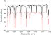 |
Fig. 1 Thick black line: spectrum of Mars between 1236 and 1242 cm-1, integrated over the Martian disk, recorded on July 3, 2014 (Ls = 156°, normalized radiance). Thick red line (in absolute units shifted by −0.30): Transmission from the terrestrial atmosphere, computed with the Gemini Observatory model (H2O = 1 pr-mm). |
Observations took place during two runs: (1) March 1, 2014, 12:00−14:00 UT (Ls = 96°, near northern summer solstice) and (2) July 2−4, 2014, 16:00−19:00 UT (Ls = 156°, middle of northern summer). The diameter of Mars was 11.6 arcsec and 9.4 arcsec in March and July respectively, so in both cases we scanned the northern and the southern hemispheres successively to obtain a full map. The time needed to record a full map, including both hemispheres, was about 15 min. An example of disk-integrated spectrum, corresponding to a two-hour integrating time on July 3, 2014, is shown in Fig. 1. Doppler velocities were −13.4 km s-1 and +11.5 km s-1 on March 1, 2014 and July 3, 2014 corresponding (at 1240 cm-1) to Doppler shifts of +0.054 cm-1 and −0.0475 cm-1, respectively. The TEXES data cubes are calibrated using the radiometric method commonly used for submillimeter/millimeter astronomy (Rohlfs & Wilson 2004), which is described in detail in Lacy et al. (2002).
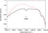 |
Fig. 2 Thick black line: HDO transition on Mars between 1236.15 and 1236.45 cm-1, integrated over the Martian disk, recorded on July 3, 2014 (Ls = 156°, normalized radiance). Thick red line: normalized atmospheric transmission as measured by the TEXES instrument. |
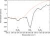 |
Fig. 3 Thick black line: H2O2 transitions on Mars between 1241.50 and 1241.65 cm-1, integrated over the Martian disk, recorded on July 3, 2014 (Ls = 156°, normalized radiance). Thick red line: Normalized atmospheric transmission as measured by the TEXES instrument. |
For both datasets, the Martian disks had a comparable size (about 10 arcsec) and a high illumination factor (above 87%), but the local times were very different. In March 2014 the evening terminator was observed, while in July 2014 the morning terminator was in the field of view. This latter configuration (observation of a significant night crescent and morning terminator) was not observed in any of our previous runs (Encrenaz et al. 2012). As will be discussed below, this has an important effect on the structure of the thermal profile before and around dawn, and on our ability to retrieve mixing ratios of minor species.
As in the case of our previous observations, we selected weak transitions of HDO, H2O2 and CO2, well isolated from telluric lines. In the case of HDO, we selected transitions at 1237.077 cm-1 ([0 1 0, 4 3 2]−[0 0 0, 5 4 1]; I = 6.49 × 10⁻²⁴ cm molec-1, E = 480.259 cm-1) and 1236.295 cm-1 ([0 1 0, 5 2 4]−[0 0 0, 6 3 3]; I = 3.90 × 10⁻²⁴ cm molec-1, E = 469.664 cm-1) in March and July respectively. Figure 2 shows the 1236.3 cm-1 transition of HDO integrated over the disk on July 3. The 1237.08 cm-1 transition was not usable in the July data owing to an instrumental spike that occurred exactly at this frequency. Both HDO lines have intensities corresponding to line depths of a few percent. For both runs we used the H2O2 doublet of the ν6 band at 1241.533 cm-1 (I = 3.600 × 10⁻²⁰ cm molec-1, E = 155.502 cm-1) and 1241.613 cm-1 (I = 3.370 × 10⁻²⁰ cm molec-1, E = 163.185 cm-1), which brackets a weak CO2 isotopic (628) transition at 1241.58 cm-1 (Fig. 3); the CO2 line is a very close doublet at 1241.574 cm-1 and 1241.580 cm-1, (with I = 5.200 × 10⁻²⁷ cm molec-1 and E = 664.59 cm-1 for each transition). In Figs. 2 and 3, the atmospheric transmission, as observed by the TEXES instrument, is shown for comparison. For both lines it can be seen that the shape of the continuum, on both sides of the lines, shows the same trend as the atmospheric transmission. However, the fit is not good enough to correct the continuum fluctuations by making the ratio of the Mars spectrum by the atmospheric transmission curve, implying that additional fluctuations of instrumental origin remain in the continuum. It can be seen from the data that these fluctuations are not constant over the disk but vary from pixel to pixel. Given lack of accurate modeling of these fluctuations, we have measured the line depths by using, for the continuum of each line, a straight line between the continuum fluxes measured on each side of this line. This simple method has the advantage of making no a priori assumption on the nature of the fluctuations.
The HDO and H2O2 mixing ratios were estimated from the ratios of the line depths of the HDO and H2O2 lines divided by the CO2 line depth. As discussed in earlier papers (see Encrenaz et al. 2008), this first-order method minimizes the uncertainties associated with the surface and atmospheric parameters, as well as the airmass factor. In the present paper, we present a full analysis of the uncertainties associated with this method (see Sect. 3.3 and Appendix). Other uncertainty sources (noise level, calibration accuracy, pointing and limb positioning accuracy) are also discussed below (Sects. 3.1.1, 3.2.1 and 3.3). As in our previous studies, our mixing ratios, expressed by volume, are derived relative to carbon dioxide.
2.2. Data interpretation and modeling
The continuum radiance (at 1341.6 cm-1) and the line depths of the selected transitions were measured in each pixel, and maps of these parameters were extracted from the data cubes. Maps of the line depth ratios were obtained in all regions of the Martian disk where (1) the continuum level was significantly above the noise level (larger than 5 erg/s/cm2/sr/cm-1), and (2) the CO2 line depth was positive and above the noise level (larger than 0.02). Our criteria excluded the regions where the temperature profile is quasi-isothermal or even shows an inversion. As will be presented below, this case happens late in the evening in the case of the March observations, and on the night side and at dawn near the morning terminator in the case of the July observations. We decided to also remove the regions on the night side where both the CO2 and the minor species showed emission lines because there may be some uncertainty if lines are formed at slightly different altitude levels.
On the basis of the maps, we selected regions where the HDO and H2O2 mixing ratios were highest, and compared the spectra in these regions with synthetic models. As a first guess, we used the atmospheric parameters (surface pressure, surface temperature, and thermal profile) inferred from the Global Climate Model (GCM, Forget et al. 1999). We then used the CO2 transitions to get the best fit by slightly adjusting these parameters, and we used them to model the HDO and H2O2 transitions. Calculations show that for all transitions the lines are mostly formed in the lower troposphere, within the first ten kilometers above the surface.
Our synthetic spectra were modeled using spectroscopic data extracted from the GEISA molecular database (Jacquinet-Husson et al. 2008). In addition, weak CO2 isotopic transitions were added using the analysis of Rothman (1986). In the case of HDO, water vapor was inferred in a next step, assuming a Martian D/H mixing ratio of 5 times the terrestrial value, on the basis of previous observational estimates (this assumption is discussed in more detail in Sect. 4.2). We note, however, that this ratio is expected to show variations over the Martian disk with latitude and season (Montmessin et al. 2005; Novak et al. 2012; Villanueva et al. 2015), and a more accurate measurement of the D/H ratio on Mars for all seasons remains to be achieved.
As in our previous analyses, we have assumed for both H2O and H2O2 a constant mixing ratio as a function of altitude. The spectral resolution of TEXES does not allow us to have access to the true profiles of the minor species; only heterodyne spectroscopy with a resolving power of 106 would deliver this information. In addition, the line depth ratio method gives the measurement of the mixing ratios of the minor species versus CO2 assuming the same scale height for all molecules. The consequences of this approximation are analyzed in the discussion (Sects. 4.1.4 and 4.2.3).
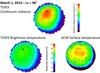 |
Fig. 4 Top: continuum radiance map of the Martian disk recorded at 1241.50 cm-1 on March 1, 2014 (Ls = 96°). Bottom left: brightness temperature TEXES map converted from the radiance map, assuming a surface emissivity of 1.0. The subsolar point is indicated with a white dot. The black circle corresponds to Region A where the TEXES spectra were modeled (see text). Bottom right: synthetic map of the surface temperature retrieved from the GCM under similar observing conditions. |
3. Results
3.1. Northern summer solstice (Ls = 96°, March 1, 2014)
3.1.1. Continuum radiance and surface temperature
Figure 4 shows a map of the continuum radiance, measured at 1241.50 cm-1. We convert the radiance into brightness temperature to compare it with a map of the surface temperature for the same date and under the same geometrical conditions extracted from the GCM. Assuming no extinction by dust and clouds, the continuum radiance gives us the product ϵ× BB(Ts), where BB(Ts) is the blackbody corresponding to the surface temperature and ϵ is the surface emissivity. Comparison of this quantity with the predicted GCM surface temperature gives us information about the surface emissivity and the possible extinction from the atmosphere (dust and clouds).
It can be seen that the two maps are in good agreement in terms of global distribution over the disk. However, in the region of maximum flux, the TEXES brightness temperature is lower than the GCM prediction by about 20 K, corresponding to a decrease in radiance of about 60%. The difference between the TEXES brightness temperature and the GCM surface temperature can be due to three factors: the surface emissivity ϵ, the extinction by airborne dust and the extinction by water ice clouds. The surface emissivity at 1240 cm-1 is known to be higher than 0.90 (Christensen et al. 2001). The dust opacity in the northern hemisphere for Ls = 96° is expected to be very low (Smith 2004). In contrast, the presence of water ice clouds is likely in this season, especially for low and middle latitudes (Smith 2004). Thus, the difference between the observed and expected radiances in the region of maximum is most likely the result of cloud extinction. As this effect acts as a gray screen at high altitude (above the lower troposphere where the lines are formed), it is not expected to affect the line depths of the spectrum, and a fortiori their line depth ratios.
3.1.2. H2O2 and HDO mixing ratios
Figure 5 shows the maps of the line depths of CO2 (1241.58 cm-1), HDO (1237.08 cm-1) and H2O2 (1241.53 cm-1). The CO2 map indicates a maximum in the northern hemisphere in the morning and around noon. It illustrates both a maximum of the surface temperature in this region as shown in Fig. 4 and an airmass effect at the morning limb, also associated with a topography effect. These maps, together with Fig. 4, indicate the regions of the Martian disk where the HDO and H2O2 mixing ratios can be retrieved; the evening regions and the night side are excluded because the continuum is too low.
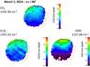 |
Fig. 5 Maps of the line depths for CO2 (1241.58 cm-1), HDO (1237.07 cm-1) and H2O2 (1241.53 cm-1) recorded on March 1, 2014 (Ls = 96°). The measurement is not reliable at the evening terminator and on the night side because the continuum is too low. |
H 2 O 2
Figure 6 shows a map of the H2O2/CO2 line depth ratio, retrieved from the TEXES maps shown in Fig. 5. As explained in detail in the Appendix, in the case of H2O2, the line depth ratio can be converted into the mixing ratio of the molecule with an accuracy of a few percent all over the disk. We convert this unit into the H2O2 mixing ratio per volume, using the relationship ![Mathematical equation: \begin{eqnarray*} \rm mr(H_2O_2) = ldr(H_2O_2) \times 40./0.29 / [1.0 + (am - 1.0)\times 0.025], \end{eqnarray*}](/articles/aa/full_html/2015/06/aa25448-14/aa25448-14-eq27.png) where mr is the mixing ratio, ldr the line depth ratio and am the airmass. This equation, discussed in the Appendix, includes a correction for the airmass. Our map is then compared with a map of the column averaged H2O2 mixing ratio retrieved from the GCM under the same observing conditions. It can be seen that there is a good overall agreement between the two maps: as expected at the time of northern summer solstice, the hydrogen peroxide content is highest at high northern latitudes with a mixing ratio of about 30−40 ppbv. We note, however, a discrepancy in the fine structure of the H2O2 spatial distribution in this region: the TEXES data indicate a maximum around the pole while the GCM predicts a maximum at latitudes around 60N.
where mr is the mixing ratio, ldr the line depth ratio and am the airmass. This equation, discussed in the Appendix, includes a correction for the airmass. Our map is then compared with a map of the column averaged H2O2 mixing ratio retrieved from the GCM under the same observing conditions. It can be seen that there is a good overall agreement between the two maps: as expected at the time of northern summer solstice, the hydrogen peroxide content is highest at high northern latitudes with a mixing ratio of about 30−40 ppbv. We note, however, a discrepancy in the fine structure of the H2O2 spatial distribution in this region: the TEXES data indicate a maximum around the pole while the GCM predicts a maximum at latitudes around 60N.
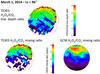 |
Fig. 6 Top: map of the line depth ratio of H2O2/CO2 retrieved from the TEXES data recorded on March 1, 2014 (Ls = 96°). The black circle corresponds to region A where the TEXES spectra were modeled (see text). Bottom left: map of the TEXES H2O2/CO2 mixing ratio, in ppbv, derived from the H2O2/CO2 line depth ratio. Bottom right: GCM synthetic map of the H2O2/CO2 column-averaged mixing ratio calculated for the same observing conditions. |
Following the method developed in previous studies (Encrenaz et al. 2004; 2005; 2012), we used the TEXES map of H2O2 to isolate a region at high northern latitude (region A) corresponding to a high H2O2 content. Area A, located around 50N at a local time of 13:00, is chosen near noon in order to maximize the continuum level and to optimize the signal-to-noise ratio of the data. We modeled the H2O2 and CO2 lines in this region to infer the hydrogen peroxide content. Starting from the GCM atmospheric parameters corresponding to this region and using the appropriate air mass, we first adjusted these parameters to fit the CO2 transition at 1241.58 cm-1. Our thermal profile has temperatures of 236 K, 205 K, 166 K and 155 K at altitudes of 0 km, 10 km, 30 km, and 50 km, respectively. We used a surface pressure of 8.3 mbar and a surface brightness temperature of 250 K. This profile is also shown in the Appendix (Fig. 17). Then, we adjusted the H2O2 mixing ratio to fit the H2O2 doublet. The result is shown in Fig. 7. It can be seen that the best fit corresponds to a H2O2 mixing ratio of 20 ppbv. This result is discusssed and compared with 3D-photochemical simulations in Sect. 4.
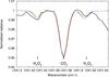 |
Fig. 7 Thick black line: TEXES spectrum of Mars in the vicinity of H2O2 and CO2 lines around 1241.58 cm-1 (March 1, 2014, Ls = 96°), integrated over Region A (9 pixels), compared with synthetic spectra. The continuum fluctuation in the TEXES data was corrected by using the continuum on each side of each line and assuming a straight line between these two points. The airmass is 1.20. Models: H2O2 = 15 ppbv (green), 20 ppbv (red), 25 ppbv (blue). The best fit is obtained for H2O2 = 20 ppbv. |
HDO
Figure 8 shows a map of the HDO/CO2 line depth ratio, retrieved from the TEXES maps shown in Fig. 4 and a map of the HDO mixing ratio calculated using the formula  where mr is the mixing ratio and ldr the line depth ratio (see Appendix). Then we compare this map with a map of the HDO column density retrieved from the GCM and the simulations of Montmessin et al. (2005) under the same observing conditions. These maps are discussed in Sect. 4.
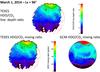 |
Fig. 8 Top: map of the line depth ratio of HDO/CO2 retrieved from the TEXES data recorded on March 1, 2014 (Ls = 96°). The black circle corresponds to Region A where the TEXES spectra were modeled (see text). Bottom left: TEXES map of the HDO/CO2 mixing ratio inferred from the HDO/CO2 line depth ratio. Bottom right: GCM synthetic map of the HDO mixing ratio, in ppbv, under the same observing conditions. |
We used the same area as defined above to infer the HDO water content at high northern latitude (Area A). We modeled the HDO spectrum using the surface parameters, the thermal profile, and the airmass factor defined for the H2O2 study. The result is shown in Fig. 9. The best fit is obtained for a HDO mixing ratio of 450 ppbv, corresponding to a column density of 45 pr-nm. This result is discussed in Sect. 4.
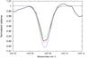 |
Fig. 9 Thick black line: TEXES spectrum of Mars near the HDO line in the vicinity of 1237.08 cm-1, integrated over Region A (9 pixels), compared with synthetic spectra (March 1, 2014; Ls = 96°). The continuum fluctuation in the TEXES data has been corrected by using the continuum on each side of each line and assuming a straight line between these two points. The airmass is 1.20. Models: H2O = 375 ppbv (green), 450 ppbv (red), 525 ppbv (blue). The best fit is obtained for HDO = 450 ppbv. |
3.2. Southern summer (Ls = 156°, July 3, 2014)
Data were recorded over three successive nights (July 2, 3, and 4, 2014, between 16:00 and 19:00 UT). Data cubes were acquired over the disk of Mars in the 1236−1242 cm-1 range. Maps of the continuum radiance and the line depths of CO2, HDO and H2O2 were very similar over the three nights, leading to identical maps of the H2O2 and HDO mixing ratios. We present below the results obtained on July 3, 2014.
3.2.1. Continuum radiance and surface temperature
Figure 10 shows the continuum radiance map of Mars for July 3, 2014. This map is converted in brightness temperature and compared with a map of the surface temperature extracted from the GCM under the same observing conditions. As in the case of the March data, the general agreement is good, except near the limb in the afternoon where the maximum radiance expected in the GCM is not observed by TEXES. We note that, in the case of the TEXES map, there may be an uncertainty associated with the definition of the limb; because of the low temperatures on the night side, the map was far from being spherical. The limb was defined using both the continuum and the CO2 line depth maps; however, the precision was limited by the quality of the seeing (not better than 1 arcsec), which translates into about two hours in local time at the limb near the equator. More important, the convolution by the 1-arcsec seeing has the effect of decreasing the flux in the limb pixels, which explains most of the difference between the TEXES and GCM maps at the limb. We also note that in southern summer (Ls = 156°) some dust may be expected in the atmosphere (Smith 2004). Clouds and dust extinction, associated with the high airmass, are probably responsible for the observed cooling near the limb, not predicted in the GCM surface temperature map. As in the case of the March 2014 data, the extinction by dust and/or clouds should have no incidence on the retrieval of the H2O2 and HDO mixing ratios.
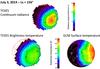 |
Fig. 10 Top: continuum radiance map of the Martian disk recorded at 1241.50 cm-1 on July 3, 2014 (Ls = 156°). Bottom left: TEXES map of the brightness temperatures inferred from the radiance map, assuming a surface emissivity of 1.0. The subsolar point is indicated with a white dot. The black circle corresponds to Region B where the TEXES spectra were modeled (see text). Bottom right: synthetic map of the surface temperature retrieved from the GCM under similar observing conditions. |
3.2.2. H2O2 and HDO mixing ratios
Figure 11 shows the maps of the line depths of CO2 (1241.58 cm-1), HDO (1236.30 cm-1), and H2O2 (1241.53 cm-1). The CO2 map indicates a maximum around noon and in the afternoon. It illustrates both a maximum of the surface temperature in this region (Fig. 10), hence a maximum temperature contrast between the surface and the atmosphere, and an airmass effect at the afternoon limb. On the night side and near dawn, the HDO and H2O2 mixing ratios cannot be retrieved because the continuum is too low and the CO2 line depth is too weak.
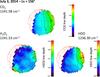 |
Fig. 11 Maps of the line depth of CO2 (1241.58 cm-1), HDO (1236.30 cm-1) and H2O2 (1241.53 cm-1) recorded on July 3, 2014 (Ls = 156°). The measurement is not reliable on the night side or near dawn because the continuum is too low. |
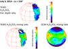 |
Fig. 12 Top: map of the line depth ratio of H2O2/CO2 retrieved from the TEXES data recorded on July 3, 2014 (Ls = 156°). The black circle corresponds to Region B where the TEXES spectra were modeled (see text). Bottom left: map of the TEXES H2O2/CO2 mixing ratio, inferred from the H2O2/CO2 line depth ratio map. Bottom right: GCM synthetic map of the H2O2 column-averaged mixing ratio calculated for the same observing conditions. |
H 2 O 2
Figure 12 shows a map of the H2O2/CO2 mixing ratio inferred from the line depths shown in Fig. 11. The map is translated into H2O2 mixing ratios, using the formula given in the Appendix, and compared with the GCM map corresponding to the same observing conditions. Unfortunately, the TEXES map is limited to a small portion of the Martian disk, because the CO2 line depth, and a fortiori the H2O2 line depth, are close to zero for all local times earlier than 11:00 am. In the region of the disk where the H2O2 content can be measured, the agreement with the GCM map is good, with a local maximum around 35 ppbv in the afternoon (near the limb) between 0N and 30N latitude.
We have identified an area (B) corresponding to a high abundance of hydrogen peroxide. Region B corresponds to 15N–30N latitudes and a local hour of 13:00−15:00 pm. Figure 13 shows the TEXES spectrum integrated over this area, compared with synthetic models calculated using the method described above. The temperature profile used for Area B has temperatures of 241 K, 220 K, 173.5 K, and 159 K at altitudes of 0 km, 10 km, 30 km, and 50 km respectively. The surface pressure is 5.4 mbar and the surface brightness temperature is 265 K; the profile is also shown in the Appendix (Fig. 17). Figure 13 shows that the best fit is obtained for a H2O2 mixing ratio of 30 ppbv. This result is discussed below (Sect. 4).
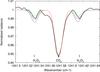 |
Fig. 13 Thick black line: TEXES spectrum of Mars in the vicinity of the H2O2 and CO2 around 1241.58 cm-1 (July 3, 2014), integrated over Region B (9 pixels), compared with synthetic spectra (July 3, 2014; Ls = 156°). The continuum fluctuation in the TEXES data has been corrected by using the continuum on each side of each line and assuming a straight line between these two points. The airmass is 1.55. Models: H2O2 = 20 ppbv (green), 30 ppbv (red), 40 ppbv (blue). The best fit is obtained for H2O2 = 30 ppbv. |
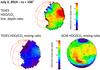 |
Fig. 14 Top: map of the line depth ratio of HDO/CO2 retrieved from the TEXES data recorded on July 3, 2014 (Ls = 156°). The black circle corresponds to region B where the TEXES spectra were modeled (see text). Bottom left: TEXES map of the HDO/CO2 mixing ratio inferred from the HDO/CO2 line depth ratio. Bottom right: GCM synthetic map of the HDO mixing ratio (ppbv) calculated for the same observing conditions. |
HDO
Figure 14 shows a map of the HDO/CO2 line depth ratio inferred from the line depth maps shown in Fig. 11 (July 3, 2014), and a map of the HDO mixing ratio, using the formula described in the Appendix. This map is compared with the GCM map of the HDO mixing ratio calculated under the same observing conditions. Because the HDO transition is significantly stronger than the H2O2 doublet, the map can be retrieved on a larger fraction of the disk (more than 50%), from about 08:00 am to 15:00 pm in local time. Comparison between the TEXES and GCM maps is discussed in Sect. 4.
Figure 15 shows a comparison between the TEXES spectrum of HDO integrated over area B, and the synthetic models calculated using the atmospheric parameters used for the fit of the H2O2 doublet. The best fit is obtained for a HDO mixing ratio of 375 ppbv, corresponding to a column density of 22 pr-nm. At this position, the GCM HDO map indicates a mixing ratio of about 600 ppbv (Fig. 14). This difference is discussed below (Sect. 4).
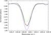 |
Fig. 15 Thick black line: TEXES spectrum of Mars in the vicinity of the HDO line at 1236.295 cm-1 (July 3, 2014; Ls = 156°), integrated over 9 pixels in region B, compared with synthetic spectra. The continuum fluctuation in the TEXES data has been corrected by using the continuum on each side of each line and assuming a straight line between these two points. The airmass is 1.55. Models: H2O = 300 ppbv (green), 375 ppbv (red), 450 ppbv (blue). The best fit is obtained for H2O = 375 ppbv. |
3.3. Uncertainty analysis
In this section, we evaluate the uncertainty associated with the determination of the H2O2 and HDO mixing ratios.
In the case of the maps of the mixing ratios (Figs. 6, 8, 12, and 14), the uncertainty associated with the method consisting of simply making the ratios of the H2O2 and HDO line depths to the CO2 line depth was first discussed in Encrenaz et al. (2008), and is analyzed in detail in the enclosed Appendix. Comparison with a grid of models covering a wide range of atmospheric parameters shows that the difference between the mixing ratio inferred from our method, compared with the mixing ratio derived from synthetic spectrum calculation, is no more than a few percent in most of the cases. In the case of H2O2, the departure due to the airmass is linear with the quantity (am −1.0) with, at the limb, a value of 10%. This departure has been corrected (Figs. 6 and 11). In the case of HDO, the departure varies as a function of the H2O mixing ratio but is always less than 10% all over the disk (airmass lower than 3) and less than 20% at the limb (see Appendix).
In the case of the spectral fits (Figs. 7, 9, 13 and 15), we first estimated the noise level in the continuum of the spectra. From Figs. 2 and 3, which show the TEXES spectrum integrated over the Martian disk, we measure a 3-σ (peak to peak) noise of 6 × 10⁻³ at the HDO line and 5 × 10⁻³ at the H2O2 line. In the case of the A and B spectra, the continuum is about 15 times lower, which translates into σ values equal to 4.5 × 10⁻³ and 4.0 × 10⁻³ respectively. Our σ estimates translate into mixing ratio fluctuations of 10 ppbv for H2O2 (Figs. 8 and 13) and 60 ppbv for HDO (Figs. 8 and 15). Taking into account the fact that we have two H2O2 lines, our results are the following:
Region A (March 1, 2014): H2O2 = 20+/−7 ppbv, HDO = 450+/−60 ppbv (45+/−6 pr-nm);
Region B (July 3, 2014): H2O2 = 30+/−7 ppbv, HDO = 375+/−60 ppbv (22+/−2.5 pr-nm).
We note that our H2O2 error bars are consistent with the limited quality of the fits (Figs. 8 and 13). Part of the misfit is due to a slight shift in the position of the H2O2 line at 1241.615, already noticed in our first analysis (Encrenaz et al. 2004) but other discrepancies, not fully understood, appear between the observed and modeled spectrum. In contrast, the two HDO fits are more satisfactory (Figs. 8 and 15). We note that the error bars derived from the signal-to-noise ratio of the TEXES data range between 23 and 35% for H2O2 and between 13 and 16% for HDO. In the case of H2O2, the error introduced by the use of the line depth ratio method is thus negligible as compared with the total error. In the case of HDO, adding quadratically an error of 10% to the uncertainties mentioned above, we derive the following values:
Region A (March 1, 2014): HDO = 450+/−75 ppbv (45+/−8 pr-nm);
Region B (July 3, 2014): HDO = 375+/−70 ppbv (22+/−3 pr-nm).
4. Discussion
4.1. Hydrogen peroxide
4.1.1. March 1, 2014 (Ls = 96°)
The spatial distribution of H2O2 inferred by TEXES is in good general agreement with the GCM prediction, with a clear enhancement toward northern latitudes as expected at the time of northern summer solstice. There is, however, a discrepancy in the exact location of the maximum, which peaks at the north pole on the TEXES map while the GCM predicts a maximum at 60N latitude. This discrepancy cannot be due to the seeing effect of the TEXES data as this effect, in contrast, tends to lower the observed flux at the limb. This difference is confirmed by the H2O2 mixing ratio measured in region A (20+/−7 ppbv), which is weaker than the predicted GCM value (30−35 ppbv). This discrepancy is presently unexplained.
4.1.2. July 3, 2014 (Ls = 156°)
According to GCM models, this is the season corresponding to the maximum global abundance of H2O2 at low latitudes (Lefèvre et al. 2008; Encrenaz et al. 2012). In the case of the July 3 observations, the H2O2 maximum calculated by the model is located around 30N latitude at both northern limbs. As explained above, the nightside limb is not accessible to observations, so the northern sunlit limb is the only place where TEXES data can be compared with GCM predictions.
The H2O2 mixing ratio derived in site B (30+/−7 ppbv, Fig. 13) is in good agreement with the GCM model, and the GCM map is also in agreement with the spatial distribution observed in this area (Fig. 12). The depletion of hydrogen peroxide toward the north pole and toward southern latitudes, expected from the GCM, is also observed in the TEXES data.
4.1.3. Seasonal variations of hydrogen peroxide
Seasonal variations of hydrogen peroxide, recorded with TEXES and other means (JCMT, Herschel/HIFI) between 2004 and 2010, were shown in Encrenaz et al. (2012). Northern latitudes (around a mean value of 20N) were observed during northern spring and summer, while southern latitudes around 20S were observed during northern autumn and winter. Results were compared with various photochemical models, including the 1D models of Moudden (2007) and Krasnopolsky (2009), and the GCM models developed assuming both homogeneous and heterogeneous chemistry. Our conclusion was that the observed data was in better agreement with the GCM heterogeneous model (Lefèvre et al. 2008; Encrenaz et al. 2012). However, no data were recorded between Ls = 120° and Ls = 180°, a season critical for distinguishing between different photochemical models.
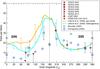 |
Fig. 16 Seasonal cycle of hydrogen peroxide on Mars integrated over the Martian disk. Observed regions are centered around 20N during northern spring and summer, and around 20S during northern autumn and winter. Yellow: 3D GCM model considering only the gas phase. Blue: 3D GCM model considering heterogeneous chemistry on water ice grains. Blue circles: 1D model by Krasnopolsky (2009). Green squares: 1D model by Moudden (2007). The figure has been updated from Lefèvre et al. (2008) and Encrenaz et al. (2012). |
The July 2014 data help us to fill this gap, while the March 2014 data provide a new point around northern summer solstice, also critical for distinguishing among models, for which contradictory results were obtained in the past. In the case of the March 2014 data, using Fig. 6, we first estimate a mean mixing ratio over the 20N latitude range, noting that the disk center actually corresponds to this latitude. We derive a H2O2 disk-averaged mixing ratio of 15+/−7 ppb, in good agreement with the GCM value. In the case of the July 2014 data, we cannot estimate the mean TEXES value for a latitude of 20N but, based on the good agreement of TEXES with the GCM in Region B, from the GCM map we use a mean value of 30+/−7 ppbv over the 20N latitude range.
Figure 16 shows the mean 20N and 20S variations of H2O2 as a function of the areocentric longitude Ls updated from the work of Lefèvre et al. (2008) and Encrenaz et al. (2012). It can be seen that, in spite of the relatively large error bars of the data and the models, the two new data points obtained in 2014 favor the heterogeneous model developed by Lefèvre et al. (2008). This model, initially based on the seasonal behavior of ozone in the Earth, was able to reproduce the ozone seasonal cycle on Mars, assuming that water ice clouds provide sites for uptaking ozone-destroying hydrogen radicals HOx. This mechanism leads to H2O2 abundances that are lower than in a simulation that only takes into account gas-phase chemistry.
The difference between the H2O2 contents in the homogeneous and heterogeneous chemistry models may be visible on their disk-integrated mixing ratios, as shown in Fig. 16, and also in their spatial distribution over the disk. For Ls = 96° (March 2014), the ice clouds are expected to be at a maximum near the equator (Smith 2004), and so is the depletion of H2O2 in the heterogeneous model (Fig. 16). Such a depletion, with respect to higher northern latitudes, is actually observed with TEXES (Fig. 6). For Ls = 156°, in contrast, the water ice depletion at the equator is much less (Smith 2004), and the H2O2 depletion due to reactions on ice near the equator is much less pronounced, both from the observation (Fig. 12) and in the GCM (Fig. 16).
In spite of their relatively large error bars, the new TEXES data provide additional support to the heterogeneous chemistry model. A puzzling question remains, however: the upper limit of 3 ppbv recorded by Herschel/HIFI for Ls = 77° (Hartogh et al. 2010) remains unexplained. The upper limit recorded by TEXES for Ls = 112° (10 ppbv, Encrenaz et al. 2002) is also surprising; however, the time exposure for this dataset was quite short, so the data quality was significantly lower than for the following runs. Nevertheless, there are still possibly interannual variations of hydrogen peroxide that need to be better understood.
4.1.4. Vertical distribution of hydrogen peroxide
As mentioned above, we have assumed in our study a constant vertical mixing ratio for hydrogen peroxide. However, photochemical models predict that H2O2 is essentially confined near the surface as it mimics the water behavior as a function of season (Clancy & Nair 1996; Lefèvre et al. 2004; Encrenaz et al. 2012), following the variations of the hygropause which is quite low at both of the seasons observed here. As a result, the H2O2 mixing ratios retrieved in this study might be underestimated at the surface. However, photochemical models (Lefèvre et al. 2004) predict that the H2O2 cutoff is located between 10 and 20 km, i.e., above the region probed by TEXES. Thus, the assumption of constant mixing ratio is expected to have a minor influence on our results.
4.2. HDO and H2O
As in our previous analyses (Encrenaz et al. 2005, 2008, 2010), we have converted our HDO measurements into H2O mixing ratios for a comparison with earlier observations (Smith 2002, 2004) and GCM results. We first need to make an assumption of the mean D/H ratio on Mars. Past observations indicate mean or localized enrichments (with respect to the terrestrial value, the Standard Mean Ocean Water SMOW) of 6+/3 (Owen et al. 1989), 5.2+/−1.0 (Krasnopolsky et al. 1997), 5.0 (Hartogh et al. 2011) and 6.0+/−1.0 (Webster et al. 2013). Maps of D/H during northern spring were measured by Novak et al. (2011) and Villanueva et al. (2015) during northern spring, indicating a Martian D/H ratio around 7 times the terrestrial value; in addition, Villanueva et al. (2015) observed strong variations of the D/H ratio over the disk (from about 2 to 9 times the SMOW value). In their model of the HDO cycle, Montmessin et al. forced the north polar cap reservoir with a deuterated content of 5.6 times the terrestrial value. As a result, their mean planetary-averaged D/H ratio is 4.8, with small variations with season (about 2%) and moderate variations with latitude (about 10%), except at the poles (up to 50%).
In what follows, we convert our HDO maps using a mean D/H of 5.0 wr SMOW. This is consistent with our previous studies and allows us to compare our HDO and H2O maps with the ones produced by the GCM. However, we are aware that a more accurate determination of D/H as a function of latitude, topography, and season needs to be achieved. Figures 17 and 18 show the TEXES maps of water vapor for March 2014 and July 2014, respectively, compared with the GCM maps calculated under the same conditions.
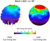 |
Fig. 17 Left: map of the H2O/CO2 mixing ratio (in ppmv) retrieved from the TEXES data recorded on March 1, 2014 (Ls = 96°), converted from the HDO/CO2 mixing ratio map (Fig. 8), assuming a Martian mean D/H ratio of 5 times the terrestrial value. The black circle corresponds to region A where the TEXES spectra were modeled (see text). Right: GCM synthetic map of the H2O2/CO2 column-averaged mixing ratio (in ppmv) calculated for the same observing conditions. |
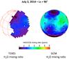 |
Fig. 18 Left: map of the H2O/CO2 mixing ratio (in ppmv) retrieved from the TEXES data recorded on July 3, 2014 (Ls = 156°), converted from the HDO/CO2 mixing ratio map (Fig. 14), assuming a Martian mean D/H ratio of 5 times the terrestrial value. The black circle corresponds to region B where the TEXES spectra were modeled (see text). Right: GCM synthetic map of the H2O2/CO2 column-averaged mixing ratio (in ppmv) calculated for the same observing conditions. |
4.2.1. March 1, 2014 (Ls = 96°)
It can be seen from Fig. 8 that the two HDO maps, from TEXES and from the GCM, are generally consistent: as expected at the time of northern summer solstice, the HDO content is maximum around the north pole. There are some differences, however. The maximum mixing ratio at the north pole, as observed by TEXES, is about 25% weaker than expected by the model. In addition, the TEXES data do not reproduce the morphology shown at low latitudes by the GCM simulation. These differences also reflect in Fig. 17 where the agreement is satisfactory for low and middle latitudes, while the excess of the predicted water content versus the TEXES measurement is about 1.5 at 30–60 northern latitudes, and up to a factor of 2 at the north pole.
4.2.2. July 3, 2014 (Ls = 156°)
Figure 14 shows that the HDO abundance measured by TEXES is significantly lower than the GCM predictions. Both TEXES and GCM maps show a maximum near the limb, in the evening and at northern mid-latitudes; however, the observed HDO mixing ratio is lower than the GCM predictions all over the observed area by about a factor of 1.5 to 2. The same discrepancy (by a factor of about 2) is observed in the H2O maps for mid-latitudes in the evening.
4.2.3. Vertical distribution of water vapor
As mentioned above (Sects. 2.2 and 4.2.4), our retrieval of the water vapor mixing ratio assumes a constant vertical value, and thus does not account for condensation, which is especially efficient near northern summer solstice, close to the cold aphelion period. We note that the same approximation was used by Smith et al. (2000) and Smith (2002) in their reduction of the TES database. This effect is expected to lead to an underestimation of the water vapor mixing ratio at the surface, while the effect of cold aerosols over the hygropause should lead to the opposite effect, so both effects are expected to compensate.
5. Conclusions
The main conclusions of the present study can be summarized as follows:
-
New TEXES observations were obtained in 2014 at the time of maximum water content (March 2014, Ls = 96°) and maximum hydrogen peroxide content at low latitudes (July 2014, Ls = 156°). Maps of H2O2 obtained with TEXES are in good overall agreement with the predictions of the Global Climate Model (GCM). Maps of HDO are generally consistent with the GCM model, but indicate lower values (by a factor of about 1.5−2) in the regions where HDO is expected to be at a maximum.
-
The new measurements of hydrogen peroxide are better fitted with the 3D GCM model which takes into account heterogeneous chemistry over water ice grains (Lefèvre et al. 2008).
-
The July 2014 dataset illustrates the dependence of the retrieval of minor species on the local time. Before and around dawn, the temperature contrast between the surface and the atmosphere is not sufficient for weak transitions of minor species to be measured with enough precision. The temperature gradient between the surface and the atmosphere tends to be the highest in the afternoon, which is the time when the abundances of minor species can best be retrieved.
Appendix A
In this Appendix, we investigate the validity of the line depth ratio method, i.e. the linearity of this parameter with the mixing ratio of the minor molecule (H2O2 and HDO). A first discussion was presented in Encrenaz et al. (2008) by considering a set of different atmospheric profiles and airmass conditions. Our conclusion was that the uncertainty associated with this method was always less than 10%, except at the limb where it could reach 25%. In the present study, we repeat this analysis and we describe it in detail, by considering more precisely the various atmospheric profiles associated with our observations. We consider first H2O2, then HDO, and we analyze separately the effects associated with the atmospheric profile and with the airmass.
Changes in the thermal profile of Mars are associated with the season and with the local hour. Our two sets of observations span different local hours: from 09:00 to 17:00 on March 1, 2014 and from 07:00 to 15:00 on July 3, 2014. Outside these time intervals, the TEXES data, if they exist, cannot be used because the continuum level is too low (Figs. 4 and 10). On the basis of past observations (Smith et al. 2015) and GCM simulations (Forget et al. 1999), we have built a grid of thermal profiles that are representative of all possible configurations within the local time ranges of our observations. These five profiles are shown in Fig. A.1 and described in the figure caption.
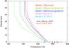 |
Fig. A.1 Thermal profiles used for the analysis of the line depth ratio method. Surface temperatures are indicated by Xs on the x-axis. A mean surface pressure of 6 mbars is assumed in all cases. The nominal profile (1, in red), with a temperature gradient of −3 K/km in the lower stratosphere and a surface temperature contrast Ts – T(0) of 40 K, is close to the GCM profile at the center of the disk in March 2014. The two next profiles (2 and 3, in green and blue) show changes in the temperature gradients from −4 K/km to −2 K/km and surface temperature contrasts of 50 K and 30 K respectively; they illustrate two extreme cases of the temperature contrast between the surface and the atmosphere. The forth profile (4), in purple, is isothermal in the first 5 km with a temperature contrast of 25 K. It corresponds to morning conditions in July 2014 and is close to the GCM profile at the center of the disk for this second run. Finally the fifth profile (5, in light blue) illustrates late afternoon conditions (LT = 17:00) for the March 2014 observations, with a temperature inversion [Ts – T(0)] of −25 K. The two profiles derived from the GCM for Areas A and B (see text, Sects. 3.1.2 and 3.2.2) are also shown in the figure (black curve: Area A; red crosses: Area B). The corresponding surface temperatures are indicated by plus signs on the x-axis. The corresponding surface pressures for Areas A and B are 8.3 mbar and 5.4 mbar, respectively. |
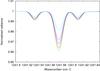 |
Fig. A.2 Spectra of the H2O2 and CO2 lines calculated with the five thermal profiles described above, for an airmass factor of 1.0 (disk.center), and for a H2O2 mixing ratio of 30 ppbv. The color code is the same as for Fig. A.1. Red: nominal model (1); green: Model 2; blue: Model 3; purple: Model 4; light blue: Model 5. The two extreme absorption cases correspond to Model 2 (maximum absorption) and Model 5 (minimum absorption). |
A.1. Hydrogen peroxide
On the basis of the H2O2/CO2 line depth ratios measured on the TEXES data and our previous measurements, we analyse how this ratio varies when the H2O2 mixing ratio varies between 0 and 40 ppbv. We consider first the effect of the thermal profiles, then the effect of the airmass.
A.1.1. Changes induced by the thermal profile
We first show in Fig. A.2 the H2O2 and CO2 spectra for our five thermal profiles, corresponding to an airmass of 1.0. As expected, the lines are strongest when the temperature contrast between the surface and the atmosphere is highest (Profile 2) and weakest in the opposite case (Profile 5). Figure A.3 shows how the H2O2/CO2 line depth ratio varies as a function of the H2O2 mixing ratio. First, it can be seen that the relation is rigorously linear up to a mixing ratio of 40 ppbv. Second, the difference between the profiles is only 3% or less, except for Profile 5 for which the line depth ratio is higher by almost 20%. This profile corresponds to a region at the limit of observability in the TEXES data of March 14 (late afternoon), where our results are limited by the weak signal of the continuum. We conclude that, in all regions where the continuum signal is strong (i.e. higher than 5 erg/s/cm-1/sr/cm-1), the uncertainty associated with changes in the thermal profile is less than a few percent. In view of the error bar on the H2O2 mixing ratio (more than 20%, see Sect. 3.3), this contribution is negligible when added quadratically with the other source (continuum noise).
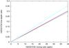 |
Fig. A.3 Variations of the H2O2 line depth ratio as a function of the H2O2 mixing ratio for the five different profiles. The color code is the same as for Figs. A.1 and A.2. All curves are exactly linear. Curves are compatible within 3% for all profiles except Profile 5 (light blue), for which the curve differs by almost 20 per cent. |
A.1.2. Changes induced by the air mass
Figure A.4 shows, in the case of the nominal model (1), the variations of the H2O2 line depth ratio as a function of the H2O2 mixing ratio for five values of the airmass (from 1.0 to 5.0). It can be seen that the departure from the am = 1 curve is linear, with a maximum value of 10% for am = 5. We have checked that the same behavior is observed for all the other profiles. It is thus possible to correct this effect by applying a correction to the observed line depth ratios. We convert the line depth ratios (ldr) into mixing ratios (mr) using the following formula: where am is the airmass. This correction is applied in Figs. 6 and 12 (we note that the difference in the maps with and without the correction is almost undetectable).
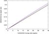 |
Fig. A.4 Variations of the H2O2 line depth ratio as a function of the H2O2 mixing ratio for the nominal profile (1), for different values of the airmass (am = 1.0, 2.0, 3.0, 4.0 and 5.0). It can be seen that the departure from the am = 1 curve is linear and proportional to the quantity (am – 1.0). |
A.2. HDO
The depths of two HDO lines used in the present study (1237.077 cm-1 in March 2014, 1236.295 cm-1 in July 2014) are deeper than the values of the H2O2 doublet. For our analysis, we use the 1237.077 cm-1 transition, which is stronger than the other by about a factor of 2. Figure A.5 shows the spectra of this HDO line calculated for the five profiles considered above, for an air mass of 1.0. Figure A.5 shows the same trend as in the case of H2O2 (Fig. A.2), with a maximum depth corresponding to Model 2 (maximum gradient) and a minimum depth corresponding to Model 5 (17:00 LT).
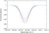 |
Fig. A.5 Spectra of the HDO line at 1237.077 cm-1, calculated with the five thermal profiles described above, for an airmass factor of 1.0 (disk.center). The color code is the same as for Fig. A.1. Red: nominal model (1); green: Model 2; blue: Model 3; purple: Model 4; light blue: Model 5. The two extreme absorption cases correspond to Model 2 (maximum absorption) and Model 5 (minimum absorption). |
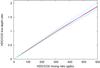 |
Fig. A.6 Variations of the HDO line depth ratio as a function of the HDO mixing ratio for the five different profiles. All curves are close to linear within 2%. Models 2 (maximum surface-atmosphere temperature contrast) and 5 (minimum surface-atmosphere temperature contrast) represent the two extreme cases. |
Figure A.6 shows, for the five atmospheric models, the variation of the HDO/CO2 line depth ratio as a function of the HDO mixing ratio, for an airmass value of 1.0. All curves are close to linearity within less than 2%. Three models (1, 3, 4) are close to the nominal profile by less than 2%, while Profiles 2 and 5 differ by about 6% with respect to the nominal profile. We can thus conclude that the error induced by the atmospheric model is in all cases less than 10%. To convert the HDO line depth ratio into a HDO mixing ratio, we used the following formula, derived from Fig. A.6:  Figure A.7 shows the variations of the HDO/CO2 line depth ratio as a function of the HDO mixing ratio for different values of the airmass. It is interesting to see that the behavior is different from the H2O2 case, in that the HDO/CO2 line depth ratio is usually stronger than the H2O2/CO2 line depth ratio. For weak values of the HDO mixing ratio (lower than 150 ppbv), the slopes of the curves are, as for H2O2, proportional to the factor (am – 1), with am being the airmass. However, when the HDO/CO2 line depth ratio comes close to about 0.8, all curves converge to a single point (for a HDO mixing ratio which slightly depends upon the model used) and diverge again for higher values of the HDO mixing ratio.
The maximum departure from linearity is 20% for an air mass of 5.0, in the case of a HD0 mixing ratio of 600 ppbv (higher than the values measured in our observations). In the case of the TEXES observations, with a disk diameter of 10 arcsec, the spatial resolution of 1 arcsec does not allow us to probe the limb at an airmass higher than 3.0. We thus conclude that, for any value of the H2O mixing ratio, the maximum uncertainty induced by our method is less than 10% anywhere on the disk and less than 20% near the limb.
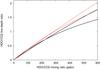 |
Fig. A.7 Variations of the HDO/CO2 line depth ratio as a function of the HDO mixing ratio for two extreme profiles (black lines: Model 2; red lines: Model 5), for two different values of the airmass (am = 1.0 and 5.0). It can be seen that, for low values of the line depth ratio, the behavior is similar to the H2O2 case (Fig. A.4). The curves converge in a single point where this ratio is close to 0.7−0.9, and diverge again for higher values of the line depth ratio. |
Acknowledgments
T.E. and T.K.G. were visiting astronomers at the Infrared Telescope Facility, which is operated by the University of Hawaii under cooperative agreement no. NNX-08AE38A with the national Aeronautics and Space Administration, Science Mission Doctorate, Planetary Astronomy Program. We wish to thank the IRTF staff for the support of TEXES observations. T.K.G. acknowledges support of NASA Grant NNX14AG34G. T.E. and B.B. acknowledge support from CNRS and Programme National de Planétologie. T.F. acknowledges support from UPMC. T.E. acknowledges support from Jet Propulsion Laboratory as a Distinguished Visiting Scientist. We are grateful to G. Villanueva for very helpful comments regarding this paper.
References
- Atreya, S. K., & Gu, Z. G. 1995, Adv. Space Res., 16, 57 [NASA ADS] [CrossRef] [Google Scholar]
- Christensen, P. R., Banfield, J. L., Hamilton, V. E., et al. 2001, J. Geophys. Res., 106, 23823 [NASA ADS] [CrossRef] [Google Scholar]
- Clancy, R. T., & Nair, H. 1996, J. Geophys. Res., 101, 12785 [NASA ADS] [CrossRef] [Google Scholar]
- Clancy, R. T., Sandor, B. J., & Moriarty-Schieven, G. H. 2004, Icarus, 168, 116 [NASA ADS] [CrossRef] [Google Scholar]
- Encrenaz, T., Greathouse, T. K., Bézard, B., et al. 2002, A&A, 396, 1037 [NASA ADS] [CrossRef] [EDP Sciences] [Google Scholar]
- Encrenaz, T., Bézard, B., Greathouse, T. K., et al. 2004, Icarus, 170, 424 [NASA ADS] [CrossRef] [Google Scholar]
- Encrenaz, T., Bézard, B., Owen, T., et al. 2005, Icarus, 179, 43 [Google Scholar]
- Encrenaz, T., Greathouse, T. K., Richter, M. J., et al. 2008, Icarus, 195, 547 [NASA ADS] [CrossRef] [Google Scholar]
- Encrenaz, T., Greathouse, T. K., Bézard, B., et al. 2010, A&A, 520, A33 [NASA ADS] [CrossRef] [EDP Sciences] [Google Scholar]
- Encrenaz, T., Greathouse, T. K., Lefèvre, F., et al. 2012, Plan. Space Sci., 68, 3 [NASA ADS] [CrossRef] [Google Scholar]
- Forget, F., Hourdin, F., Fournier, R., et al. 1999, J. Geophys. Res., 104, 24155 [NASA ADS] [CrossRef] [Google Scholar]
- Hartogh, P., Jarchow, C., Lellouch, E., et al. 2010, A&A, 521, L49 [NASA ADS] [CrossRef] [EDP Sciences] [Google Scholar]
- Hartogh, P., Jarchow, C., de Val-Borro, M., et al. 2011, Fourth International Workshop on the Mars Atmosphere: Modelling and observations, Paris, 8−11 February. Published on line at http:// www-mars-lmd.jussieu.fr/paris2011/program.html, 44 [Google Scholar]
- Jacquinet-Husson, N., Scott, N., Chedin, A., et al. 2008, J. Quant. Spectr. Rad. Transf., 109, 1043 [NASA ADS] [CrossRef] [Google Scholar]
- Krasnopolsky, V. A. 2009, Icarus, 201, 564 [NASA ADS] [CrossRef] [Google Scholar]
- Lacy, J. H., Richter, M. J., Greathouse, T. K., et al. 2002, Pub. Astron. Soc. Pac., 114, 153 [Google Scholar]
- Lefèvre, F., Lebonnois, S., Montmessin, F., & Forget, F. 2004, J. Geophys. Res., E07004, DOI: 10.1051/0004-6361/2004JE002268 [Google Scholar]
- Lefèvre, F., Bertaux, J.-L., Clancy, R. T., et al. 2008, Nature, 454, 971 [NASA ADS] [CrossRef] [PubMed] [Google Scholar]
- Montmessin, F., Fouchet, T., & Forget, F. 2005, J. Geophys. Res., 110, 03006 [Google Scholar]
- Moudden, Y. 2007, Plan. Space Sci., 55, 2137 [NASA ADS] [CrossRef] [Google Scholar]
- Novak, R. E., Mumma, M. J., & Villanueva, G. L. 2011, Plan. Space Sci., 59, 163 [NASA ADS] [CrossRef] [Google Scholar]
- Owen, T., Lutz, B. L., de Bergh, C., & Maillard, J.-P. 1989, Science, 240, 1767 [Google Scholar]
- Parkinson, T. D., & Hunten, D. M. 1972, J. Atmos. Sci., 29, 1380 [Google Scholar]
- Rothman, L. S. 1986. Appl. Opt., 25, 1795 [Google Scholar]
- Smith, M. D. 2002, J. Geophys. Res., 107, 25 [Google Scholar]
- Smith, M. D. 2004, Icarus, 167, 148 [NASA ADS] [CrossRef] [Google Scholar]
- Smith, M. D., Banfield, J. P., & Christensen, P. R. 2000, J. Geophys. Res., 105, 9589 [Google Scholar]
- Smith, M. D., Bougher, S., Encrenaz, T., Forget, F., & Kleinboehl, A. 2015, in The atmosphere and Climate of Mars (Cambridge University Press) [Google Scholar]
- Villanueva, G., Mumma, M. J., Novak, R. E., et al. 2015, Science, submitted [Google Scholar]
- Webster, C. R., Mahaffy, P. R., Flesch, G. J., et al. 2013, Science, 341, 260 [NASA ADS] [CrossRef] [Google Scholar]
All Figures
|
Fig. 1 Thick black line: spectrum of Mars between 1236 and 1242 cm-1, integrated over the Martian disk, recorded on July 3, 2014 (Ls = 156°, normalized radiance). Thick red line (in absolute units shifted by −0.30): Transmission from the terrestrial atmosphere, computed with the Gemini Observatory model (H2O = 1 pr-mm). |
| In the text | |
|
Fig. 2 Thick black line: HDO transition on Mars between 1236.15 and 1236.45 cm-1, integrated over the Martian disk, recorded on July 3, 2014 (Ls = 156°, normalized radiance). Thick red line: normalized atmospheric transmission as measured by the TEXES instrument. |
| In the text | |
|
Fig. 3 Thick black line: H2O2 transitions on Mars between 1241.50 and 1241.65 cm-1, integrated over the Martian disk, recorded on July 3, 2014 (Ls = 156°, normalized radiance). Thick red line: Normalized atmospheric transmission as measured by the TEXES instrument. |
| In the text | |
|
Fig. 4 Top: continuum radiance map of the Martian disk recorded at 1241.50 cm-1 on March 1, 2014 (Ls = 96°). Bottom left: brightness temperature TEXES map converted from the radiance map, assuming a surface emissivity of 1.0. The subsolar point is indicated with a white dot. The black circle corresponds to Region A where the TEXES spectra were modeled (see text). Bottom right: synthetic map of the surface temperature retrieved from the GCM under similar observing conditions. |
| In the text | |
|
Fig. 5 Maps of the line depths for CO2 (1241.58 cm-1), HDO (1237.07 cm-1) and H2O2 (1241.53 cm-1) recorded on March 1, 2014 (Ls = 96°). The measurement is not reliable at the evening terminator and on the night side because the continuum is too low. |
| In the text | |
|
Fig. 6 Top: map of the line depth ratio of H2O2/CO2 retrieved from the TEXES data recorded on March 1, 2014 (Ls = 96°). The black circle corresponds to region A where the TEXES spectra were modeled (see text). Bottom left: map of the TEXES H2O2/CO2 mixing ratio, in ppbv, derived from the H2O2/CO2 line depth ratio. Bottom right: GCM synthetic map of the H2O2/CO2 column-averaged mixing ratio calculated for the same observing conditions. |
| In the text | |
|
Fig. 7 Thick black line: TEXES spectrum of Mars in the vicinity of H2O2 and CO2 lines around 1241.58 cm-1 (March 1, 2014, Ls = 96°), integrated over Region A (9 pixels), compared with synthetic spectra. The continuum fluctuation in the TEXES data was corrected by using the continuum on each side of each line and assuming a straight line between these two points. The airmass is 1.20. Models: H2O2 = 15 ppbv (green), 20 ppbv (red), 25 ppbv (blue). The best fit is obtained for H2O2 = 20 ppbv. |
| In the text | |
|
Fig. 8 Top: map of the line depth ratio of HDO/CO2 retrieved from the TEXES data recorded on March 1, 2014 (Ls = 96°). The black circle corresponds to Region A where the TEXES spectra were modeled (see text). Bottom left: TEXES map of the HDO/CO2 mixing ratio inferred from the HDO/CO2 line depth ratio. Bottom right: GCM synthetic map of the HDO mixing ratio, in ppbv, under the same observing conditions. |
| In the text | |
|
Fig. 9 Thick black line: TEXES spectrum of Mars near the HDO line in the vicinity of 1237.08 cm-1, integrated over Region A (9 pixels), compared with synthetic spectra (March 1, 2014; Ls = 96°). The continuum fluctuation in the TEXES data has been corrected by using the continuum on each side of each line and assuming a straight line between these two points. The airmass is 1.20. Models: H2O = 375 ppbv (green), 450 ppbv (red), 525 ppbv (blue). The best fit is obtained for HDO = 450 ppbv. |
| In the text | |
|
Fig. 10 Top: continuum radiance map of the Martian disk recorded at 1241.50 cm-1 on July 3, 2014 (Ls = 156°). Bottom left: TEXES map of the brightness temperatures inferred from the radiance map, assuming a surface emissivity of 1.0. The subsolar point is indicated with a white dot. The black circle corresponds to Region B where the TEXES spectra were modeled (see text). Bottom right: synthetic map of the surface temperature retrieved from the GCM under similar observing conditions. |
| In the text | |
|
Fig. 11 Maps of the line depth of CO2 (1241.58 cm-1), HDO (1236.30 cm-1) and H2O2 (1241.53 cm-1) recorded on July 3, 2014 (Ls = 156°). The measurement is not reliable on the night side or near dawn because the continuum is too low. |
| In the text | |
|
Fig. 12 Top: map of the line depth ratio of H2O2/CO2 retrieved from the TEXES data recorded on July 3, 2014 (Ls = 156°). The black circle corresponds to Region B where the TEXES spectra were modeled (see text). Bottom left: map of the TEXES H2O2/CO2 mixing ratio, inferred from the H2O2/CO2 line depth ratio map. Bottom right: GCM synthetic map of the H2O2 column-averaged mixing ratio calculated for the same observing conditions. |
| In the text | |
|
Fig. 13 Thick black line: TEXES spectrum of Mars in the vicinity of the H2O2 and CO2 around 1241.58 cm-1 (July 3, 2014), integrated over Region B (9 pixels), compared with synthetic spectra (July 3, 2014; Ls = 156°). The continuum fluctuation in the TEXES data has been corrected by using the continuum on each side of each line and assuming a straight line between these two points. The airmass is 1.55. Models: H2O2 = 20 ppbv (green), 30 ppbv (red), 40 ppbv (blue). The best fit is obtained for H2O2 = 30 ppbv. |
| In the text | |
|
Fig. 14 Top: map of the line depth ratio of HDO/CO2 retrieved from the TEXES data recorded on July 3, 2014 (Ls = 156°). The black circle corresponds to region B where the TEXES spectra were modeled (see text). Bottom left: TEXES map of the HDO/CO2 mixing ratio inferred from the HDO/CO2 line depth ratio. Bottom right: GCM synthetic map of the HDO mixing ratio (ppbv) calculated for the same observing conditions. |
| In the text | |
|
Fig. 15 Thick black line: TEXES spectrum of Mars in the vicinity of the HDO line at 1236.295 cm-1 (July 3, 2014; Ls = 156°), integrated over 9 pixels in region B, compared with synthetic spectra. The continuum fluctuation in the TEXES data has been corrected by using the continuum on each side of each line and assuming a straight line between these two points. The airmass is 1.55. Models: H2O = 300 ppbv (green), 375 ppbv (red), 450 ppbv (blue). The best fit is obtained for H2O = 375 ppbv. |
| In the text | |
|
Fig. 16 Seasonal cycle of hydrogen peroxide on Mars integrated over the Martian disk. Observed regions are centered around 20N during northern spring and summer, and around 20S during northern autumn and winter. Yellow: 3D GCM model considering only the gas phase. Blue: 3D GCM model considering heterogeneous chemistry on water ice grains. Blue circles: 1D model by Krasnopolsky (2009). Green squares: 1D model by Moudden (2007). The figure has been updated from Lefèvre et al. (2008) and Encrenaz et al. (2012). |
| In the text | |
|
Fig. 17 Left: map of the H2O/CO2 mixing ratio (in ppmv) retrieved from the TEXES data recorded on March 1, 2014 (Ls = 96°), converted from the HDO/CO2 mixing ratio map (Fig. 8), assuming a Martian mean D/H ratio of 5 times the terrestrial value. The black circle corresponds to region A where the TEXES spectra were modeled (see text). Right: GCM synthetic map of the H2O2/CO2 column-averaged mixing ratio (in ppmv) calculated for the same observing conditions. |
| In the text | |
|
Fig. 18 Left: map of the H2O/CO2 mixing ratio (in ppmv) retrieved from the TEXES data recorded on July 3, 2014 (Ls = 156°), converted from the HDO/CO2 mixing ratio map (Fig. 14), assuming a Martian mean D/H ratio of 5 times the terrestrial value. The black circle corresponds to region B where the TEXES spectra were modeled (see text). Right: GCM synthetic map of the H2O2/CO2 column-averaged mixing ratio (in ppmv) calculated for the same observing conditions. |
| In the text | |
|
Fig. A.1 Thermal profiles used for the analysis of the line depth ratio method. Surface temperatures are indicated by Xs on the x-axis. A mean surface pressure of 6 mbars is assumed in all cases. The nominal profile (1, in red), with a temperature gradient of −3 K/km in the lower stratosphere and a surface temperature contrast Ts – T(0) of 40 K, is close to the GCM profile at the center of the disk in March 2014. The two next profiles (2 and 3, in green and blue) show changes in the temperature gradients from −4 K/km to −2 K/km and surface temperature contrasts of 50 K and 30 K respectively; they illustrate two extreme cases of the temperature contrast between the surface and the atmosphere. The forth profile (4), in purple, is isothermal in the first 5 km with a temperature contrast of 25 K. It corresponds to morning conditions in July 2014 and is close to the GCM profile at the center of the disk for this second run. Finally the fifth profile (5, in light blue) illustrates late afternoon conditions (LT = 17:00) for the March 2014 observations, with a temperature inversion [Ts – T(0)] of −25 K. The two profiles derived from the GCM for Areas A and B (see text, Sects. 3.1.2 and 3.2.2) are also shown in the figure (black curve: Area A; red crosses: Area B). The corresponding surface temperatures are indicated by plus signs on the x-axis. The corresponding surface pressures for Areas A and B are 8.3 mbar and 5.4 mbar, respectively. |
| In the text | |
|
Fig. A.2 Spectra of the H2O2 and CO2 lines calculated with the five thermal profiles described above, for an airmass factor of 1.0 (disk.center), and for a H2O2 mixing ratio of 30 ppbv. The color code is the same as for Fig. A.1. Red: nominal model (1); green: Model 2; blue: Model 3; purple: Model 4; light blue: Model 5. The two extreme absorption cases correspond to Model 2 (maximum absorption) and Model 5 (minimum absorption). |
| In the text | |
|
Fig. A.3 Variations of the H2O2 line depth ratio as a function of the H2O2 mixing ratio for the five different profiles. The color code is the same as for Figs. A.1 and A.2. All curves are exactly linear. Curves are compatible within 3% for all profiles except Profile 5 (light blue), for which the curve differs by almost 20 per cent. |
| In the text | |
|
Fig. A.4 Variations of the H2O2 line depth ratio as a function of the H2O2 mixing ratio for the nominal profile (1), for different values of the airmass (am = 1.0, 2.0, 3.0, 4.0 and 5.0). It can be seen that the departure from the am = 1 curve is linear and proportional to the quantity (am – 1.0). |
| In the text | |
|
Fig. A.5 Spectra of the HDO line at 1237.077 cm-1, calculated with the five thermal profiles described above, for an airmass factor of 1.0 (disk.center). The color code is the same as for Fig. A.1. Red: nominal model (1); green: Model 2; blue: Model 3; purple: Model 4; light blue: Model 5. The two extreme absorption cases correspond to Model 2 (maximum absorption) and Model 5 (minimum absorption). |
| In the text | |
|
Fig. A.6 Variations of the HDO line depth ratio as a function of the HDO mixing ratio for the five different profiles. All curves are close to linear within 2%. Models 2 (maximum surface-atmosphere temperature contrast) and 5 (minimum surface-atmosphere temperature contrast) represent the two extreme cases. |
| In the text | |
|
Fig. A.7 Variations of the HDO/CO2 line depth ratio as a function of the HDO mixing ratio for two extreme profiles (black lines: Model 2; red lines: Model 5), for two different values of the airmass (am = 1.0 and 5.0). It can be seen that, for low values of the line depth ratio, the behavior is similar to the H2O2 case (Fig. A.4). The curves converge in a single point where this ratio is close to 0.7−0.9, and diverge again for higher values of the line depth ratio. |
| In the text | |
Current usage metrics show cumulative count of Article Views (full-text article views including HTML views, PDF and ePub downloads, according to the available data) and Abstracts Views on Vision4Press platform.
Data correspond to usage on the plateform after 2015. The current usage metrics is available 48-96 hours after online publication and is updated daily on week days.
Initial download of the metrics may take a while.