| Issue |
A&A
Volume 574, February 2015
|
|
|---|---|---|
| Article Number | A59 | |
| Number of page(s) | 17 | |
| Section | Cosmology (including clusters of galaxies) | |
| DOI | https://doi.org/10.1051/0004-6361/201423969 | |
| Published online | 26 January 2015 | |
Baryon acoustic oscillations in the Lyα forest of BOSS DR11 quasars⋆
1
CEA, Centre de Saclay, IRFU,
91191
Gif-sur-Yvette,
France
e-mail:
This email address is being protected from spambots. You need JavaScript enabled to view it.
2
APC, Université Paris Diderot-Paris 7, CNRS/IN2P3, CEA,
Observatoire de Paris, 10 rue A.
Domon & L. Duquet, 75205
Paris,
France
3
Department of Physics and Astronomy, University of
California, Irvine,
CA
92697,
USA
4
Lawrence Berkeley National Laboratory,
1 Cyclotron Road, Berkeley, CA
94720,
USA
5
Brookhaven National Laboratory, 2 Center Road, Upton, NY
11973,
USA
6
Max-Planck-Institut für Astronomie, Königstuhl 17, 69117
Heidelberg,
Germany
7
Institute of Cosmology and Gravitation, Dennis Sciama Building,
University of Portsmouth, Portsmouth, PO1
3FX, UK
8
Institute for Advanced Study, Einstein Drive, Princeton, NJ
08540,
USA
9
Apache Point Observatory, PO Box 59, Sunspot, NM
88349,
USA
10
Department of Physics and Astronomy, University of
Utah, 115 S 1400 E,
Salt Lake City, UT
84112,
USA
11
Harvard-Smithsonian Center for Astrophysics, Harvard
University, 60 Garden
St., Cambridge,
MA
02138,
USA
12
Laboratoire d’Astrophysique, École polytechnique Fédérale de Lausanne,
1015
Lausanne,
Switzerland
13
Aix-Marseille Université, CNRS, LAM (Laboratoire d’Astrophysique
de Marseille) UMR 7326, 13388
Marseille,
France
14
Institució Catalana de Recerca i Estudis Avançats,
Barcelona, Catalonia,
Spain
15
Institut de Ciències del Cosmos, Universitat de Barcelona
(UB-IEEC), 08028
Barcelona, Catalonia, Spain
16
Department of Physics and Astronomy, University of
Wyoming, Laramie,
WY
82071,
USA
17
Université Paris 6 et CNRS, Institut d’Astrophysique de
Paris, 98bis Bd
Arago, 75014
Paris,
France
18
Bruce and Astrid McWilliams Center for Cosmology, Carnegie Mellon
University, Pittsburgh, PA
15213,
USA
19
Dept. of Physics, Drexel University, 3141 Chestnut Street, Philiadelphia, PA
19104,
USA
20
Department of Astronomy and Astrophysics, The Pennsylvania State
University, University
Park, PA
16802,
USA
21
Institute for Gravitation and the Cosmos, The Pennsylvania State
University, University
Park, PA
16802,
USA
22
Department of Astronomy, Ohio State University,
140 West 18th Avenue,
Columbus, OH
43210,
USA
23
Department of Astronomy and Astrophysics and the Enrico Fermi
Institute, The University of Chicago, 5640 South Ellis Avenue, Chicago, Illinois, 60615, USA
24
Observatório Nacional, Rua Gal. José Cristino 77,
RJ –20921-400
Rio de Janeiro,
Brazil
25
Laboratório Interinstitucional de e-Astronomia, – LIneA, Rua Gal.
José Cristino 77, RJ –20921-400
Rio de Janeiro,
Brazil
26
Department of Astronomy and Space Science, Sejong
University, 143-747
Seoul,
Korea
Received: 9 April 2014
Accepted: 15 October 2014
Abstract
We report a detection of the baryon acousticoscillation (BAO) feature in the flux-correlation function of the Lyα forest of high-redshift quasars with a statistical significance of five standard deviations. The study uses 137 562 quasars in the redshift range 2.1 ≤ z ≤ 3.5 from the data release 11 (DR11) of the Baryon Oscillation Spectroscopic Survey (BOSS) of SDSS-III. This sample contains three times the number of quasars used in previous studies. The measured position of the BAO peak determines the angular distance, DA(z = 2.34) and expansion rate, H(z = 2.34), both on a scale set by the sound horizon at the drag epoch, rd. We find DA/rd = 11.28 ± 0.65(1σ)+2.8-1.2 (2σ) and DH/rd = 9.18 ± 0.28(1σ) ± 0.6(2σ) where DH = c/H. The optimal combination, ~DH0.7DA0.3/rd is determined with a precision of ~2%. For the value rd = 147.4 Mpc, consistent with the cosmic microwave background power spectrum measured by Planck, we find DA(z = 2.34) = 1662 ± 96(1σ) Mpc and H(z = 2.34) = 222 ± 7(1σ) km s-1 Mpc-1. Tests with mock catalogs and variations of our analysis procedure have revealed no systematic uncertainties comparable to our statistical errors. Our results agree with the previously reported BAO measurement at the same redshift using the quasar-Lyα forest cross-correlation. The autocorrelation and cross-correlation approaches are complementary because of the quite different impact of redshift-space distortion on the two measurements. The combined constraints from the two correlation functions imply values of DA/rd that are 7% lower and 7% higher for DH/rd than the predictions of a flat ΛCDM cosmological model with the best-fit Planck parameters. With our estimated statistical errors, the significance of this discrepancy is ≈2.5σ.
Key words: cosmology: observations / dark energy / large-scale structure of Universe / cosmological parameters
Appendices are available in electronic form at http://www.aanda.org
© ESO, 2015
1. Introduction
Observation of the peak in the matter correlation function due to baryon acoustic oscillations (BAO) in the pre-recombination epoch is now an established tool to constrain cosmological models. The BAO peak at a redshift z appears at an angular separation Δθ = rd/ [ (1 + z)DA(z) ] and at a redshift separation Δz = rd/DH(z), where DA and DH = c/H are the angular and Hubble distances, and rd is the sound horizon at the drag epoch1. Measurement of the peak position at any redshift thus constrains the combinations of cosmological parameters that determine DH/rd and DA/rd.
The BAO peak has been observed primarily in the galaxy-galaxy correlation function obtained in redshift surveys. The small statistical significance of the first studies gave only constraints on DV/rd where DV is the combination DV = [ (1 + z)DA ] 2 / 3 [ zDH ] 1 / 3, which determines the peak position for the galaxy correlation function when averaged over directions with respect to the line of sight. The first measurements were at z ~ 0.3 by the SDSS (Eisenstein et al. 2005) and 2dFGRS (Cole et al. 2005) with results from the combined data set presented by Percival et al. (2010). A refined analysis using reconstruction (Eisenstein et al. 2007; Padmanabhan et al. 2009) to improve the precision DV/rd was presented by Padmanabhan et al. (2012) and Mehta et al. (2012).
Other measurements of DV/rd were made at z ~ 0.1 by the 6dFGRS (Beutler et al. 2011), at (0.4 <z< 0.8) by WiggleZ (Blake et al. 2011a), and, using galaxy clusters, at z ~ 0.3 by Veropalumbo et al. (2014). The Baryon Oscillation Spectroscopic Survey (BOSS; Dawson et al. 2013) of SDSS-III (Eisenstein et al. 2011) has presented measurements of DV/rd at z ~ 0.57 and z ~ 0.32 (Anderson et al. 2012). A measurement at z ~ 0.54 of DA/rd using BOSS photometric data was made by Seo et al. (2012).
The first combined constraints on DH/rd and DA/rd were obtained using the z ~ 0.3 SDSS data by Chuang & Wang (2012) and Xu et al. (2012). Recently, BOSS has provided precise constraints on DH/rd and DA/rd at z = 0.57 (Anderson et al. 2014; Kazin et al. 2013).
At higher redshifts, the BAO feature can be observed using absorption in the Lyα forest to trace mass, as suggested by McDonald (2003), White (2003) and McDonald & Eisenstein (2007). After the observation of the predicted large-scale correlations in early BOSS data by Slosar et al. (2011), a BAO peak in the Lyα forest correlation function was measured by BOSS in the SDSS data release DR9 (Busca et al. 2013; Slosar et al. 2013; Kirkby et al. 2013). The peak in the quasar-Lyα forest cross-correlation function was detected in the larger data sets of DR11 (Font-Ribera et al. 2014). The DR10 data are now public (Ahn et al. 2014), and the DR11 data will be made public simultaneously with the final SDSS-III data release (DR12) in late 2014.
This paper presents a new measurement of the Lyα forest autocorrelation function and uses it to study BAO at z = 2.34. It is based on the methods used by Busca et al. (2013), but introduces several improvements in the analysis. First, and most important, is a tripling of the number of quasars by using the DR11 catalog of 158 401 quasars in the redshift range 2.1 ≤ zq ≤ 3.5. Second, to further increase the statistical power we used a slightly expanded forest range as well as quasars that have damped Lyα troughs in the forest. Finally, the Busca et al. (2013) analysis was based on a decomposition of the correlation function into monopole and quadrupole components. Here, we fit the full correlation ξ(r⊥,r∥) as a function of separations perpendicular, r⊥, and parallel, r∥, to the line of sight. This more complete treatment is made possible by a more careful determination of the covariance matrix than was used by Busca et al. (2013).
Our analysis uses a fiducial cosmological model in two places. First, flux pixel pairs separated in angle and wavelength are assigned a co-moving separation (in h-1 Mpc) using the DA(z) and DH(z) calculated with the adopted parameters. Second, to determine the observed peak position, we compare our measured correlation function with a correlation function generated using CAMB (Lewis et al. 2000) as described in Kirkby et al. (2013). We adopt the same (flat) ΛCDM model as used in Busca et al. (2013), Slosar et al. (2013), and Font-Ribera et al. (2014); with the parameters given in Table 1. The fiducial model has values of DA/rd and DH/rd at z = 2.34 that differ by about 1% from the values given by the models favored by CMB data (Planck Collaboration XVI 2014; Calabrese et al. 2013) given in the second and third columns of Table 1.
This paper is organized as follows: Sect. 2 describes the DR11 data used in this analysis. Section 3 gives a brief description of the mock spectra used to test the analysis procedure; a more detailed description is given in Bautista et al. (in prep.). Section 4 presents our method of estimating the correlation function ξ(r⊥,r∥) and its associated covariance matrix. In Sect. 5 we fit the data to derive the BAO peak position parameters, DA(z = 2.34) /rd and DH(z = 2.34) /rd. Section 6 investigates possible systematic errors in the measurement. In Sect. 7 we compare our measured peak position with that measured by the Quasar-Lyα -forest cross-correlation (Font-Ribera et al. 2014) and study ΛCDM models that are consistent with these results. Section 8 concludes the paper.
Parameters of the fiducial flat ΛCDM cosmological model used for this analysis, the flat ΛCDM model derived from Planck and low-ℓ WMAP polarization data, “Planck + WP” (Planck Collaboration XVI 2014), and a flat ΛCDM model derived from the WMAP, ACT, and SPT data (Calabrese et al. 2013).
2. BOSS quasar sample and data reduction
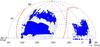 |
Fig. 1 Hammer-Aitoff projection of the BOSS DR11 footprint (Dec vs. RA). The light areas show the DR9 subregion available for the earlier studies of Busca et al. (2013) and Slosar et al. (2013). The red-dashed line shows the location of the galactic plane. |
The BOSS project (Dawson et al. 2013) of SDSS-III (Eisenstein et al. 2011) was designed to obtain the spectra of over ~1.6 × 10⁶ luminous galaxies and ~150 000 quasars. The project uses upgraded versions of the SDSS spectrographs (Smee et al. 2013) mounted on the Sloan 2.5 m telescope (Gunn et al. 2006) at Apache Point, New Mexico.
The quasar spectroscopy targets are selected from photometric data via a combination of algorithms (Richards et al. 2009; Yeche et al. 2009; Kirkpatrick et al. 2011; Bovy et al. 2011; Palanque-Delabrouille et al. 2011), as summarized in Ross et al. (2012). The algorithms use SDSS ugriz fluxes (Fukugita et al. 1996; York et al. 2000) and, for SDSS Stripe 82, photometric variability. Using the techniques of Bovy et al. (2012), we also worked with any available data from non-optical surveys: the GALEX survey (Martin et al. 2005) in the UV; the UKIDSS survey (Lawrence et al. 2007) in the NIR, and the FIRST survey (Becker et al. 1995) in the radio wavelength.
In this paper we use the data from the DR11 of SDSS-III, whose footprint is shown in Fig. 1. These data cover 8377 deg2 of the ultimate BOSS 104 deg2 footprint.
The data were reduced with the SDSS-III pipeline as described in Bolton et al. (2012). Typically, four exposures of 15 min were co-added in pixels of wavelength width Δlog 10λ = 10-4 (cΔλ/λ ~ 69 km s-1). The pipeline provides flux-calibrated spectra, object classifications (galaxy, quasar, star), and redshift estimates for all targets.
The spectra of all quasar targets were visually inspected (Pâris et al. 2012, 2014) to correct for misidentifications or inaccurate redshift determinations and to flag broad absorption lines (BALs). Damped Lyα troughs were visually flagged, but also identified and characterized automatically (Noterdaeme et al. 2012). The visual inspection of DR11 confirmed 158 401 quasars with 2.1 ≤ zq ≤ 3.5. To simplify the analysis of the Lyα forest, we discarded quasars with visually identified BALs, leaving 140 579 quasars. A further cut requiring a minimum number of unmasked forest pixels (50 analysis pixels; see below) yielded a sample of 137 562 quasars.
To measure the flux transmission, we used the rest-frame wavelength interval 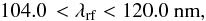 (1)slightly wider than in Busca et al. (2013). This range is bracketed by the Lyβ and Lyα emission lines at 102.5 and 121.6 nm and was chosen as the maximum range that avoids the large pixel variances on the slopes of the two lines due to quasar-to-quasar diversity of line-emission strength. The absorber redshift, z = λ/λLyα − 1, is required to be in the range 1.96 <z< 3.44. The lower limit is set by the requirement that the observed wavelength be greater than 360 nm, below which the system throughput is lower than 10% its peak value. The upper limit is produced by the maximum quasar redshift of 3.5, beyond which the BOSS surface density of quasars is not high enough to be useful for this study. The weighted distribution of redshifts of absorber pairs near the BAO peak position is shown in Fig. 2 (top panel); it has a mean of ⟨ z ⟩ = 2.34.
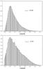 |
Fig. 2 Top: redshift distribution of pixel pairs contributing to ξ in the region 80 <r< 120 h-1 Mpc. Bottom: distribution of all pixel redshifts. |
Forests with identified DLAs were given a special treatment. All pixels where the absorption due to the DLA is higher than 20% were excluded. Otherwise, the absorption in the wings was corrected using a Voigt profile following the procedure of Noterdaeme et al. (2012). The metal lines due to absorption at the DLA redshift were masked. The lines to be masked were identified in a stack of spectra shifted to the redshift of the detected DLA. The width of the mask was 0.2 nm or 0.3 nm (depending on the line strength) or 4.1 nm for Lyβ . We also masked the ±3 nm region corresponding to Lyα if the DLA finder erroneously interpreted Lyβ absorption as Lyα absorption.
We determined the correlation function using analysis pixels that are the flux average over three adjacent pipeline pixels. Throughout the rest of this paper, “pixel” refers to analysis pixels unless otherwise stated. The width of these pixels is 207 km s-1, that is, an observed-wavelength width ~0.27 nm or ~2 h-1 Mpc. The total sample of 137 562 quasars thus provides ~2.4 × 10⁷ measurements of Lyα absorption over a total volume of ~50 h-3 Gpc3.
3. Mock quasar spectra
In addition to the BOSS spectra, we analyzed 100 sets of mock spectra. This exercise was undertaken to search for possible systematic errors in the recovered BAO peak position and to verify that uncertainties in the peak position were correctly estimated. The spectra were generated using the methods of Font-Ribera et al. (2012a). A detailed description of the production and resulting characteristics of the mock spectra is given in Bautista et al. (in prep.).
For each set of spectra, the background quasars were assigned the angular positions and redshifts of the DR11 quasars. The foreground absorption field in redshift space was generated according to a cosmology similar to the fiducial cosmology of Table 12. The unabsorbed spectra (continua) of the quasars were generated using the principal component analysis (PCA) eigenspectra of Suzuki et al. (2005), with amplitudes for each eigenspectrum randomly drawn from Gaussian distributions with sigma equal to the corresponding eigenvalues as published in Table 1 of Suzuki (2006). Finally, the spectra were modified to include the effects of the BOSS spectrograph point spread function (PSF), readout noise, photon noise, and flux systematic errors.
Our mock production pipeline admits the option of adding DLAs to the spectra according to the procedure described in Font-Ribera et al. (2012b). However, since identified DLAs are masked in the analysis of real data, we did not simulate them into the mocks. Of course, low column density and Lyman limit systems are not efficiently identified and masked in the data, which means that these systems are present in the data, but not in the mocks.
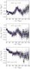 |
Fig. 3 Measured correlation function averaged over three angular regions: μ> 0.8 (top), 0.8 >μ> 0.5 (middle), and 0.5 >μ> 0.0 (bottom), where μ is the central value of |

Absorption by metals was added to a separate group of ten mocks according to the procedure described in Bautista et al. (in prep.). The quantity of each metal to be added was determined by a modified Lyα stacking procedure from Pieri et al. (2010, 2014). As discussed in Sect. 6, the metals have an effect on the recovered correlation function only at small transverse separations, r⊥< 10 h-1 Mpc, and have no significant effect on the measured position of the BAO peak.
A total of 100 independent metal-free realizations of the BOSS data were produced and analyzed with the same procedures as those for the real data. Figure 3 shows the correlation function of the mocks and the data as measured by the techniques described in the next section. The mocks reproduce the general features of the observed correlation function well. We therefore use them in Sect. 5.2 to search for biases in the analysis procedure that would influence the position of the BAO peak.
4. Measurement of the correlation function
In this section we describe the measurement of the correlation function of the transmitted flux fraction: 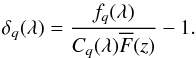 (2)Here, fq(λ) is the observed flux density for quasar q at observed wavelength λ, Cq(λ) is the unabsorbed flux density (the so-called continuum) and
  is the mean transmitted fraction at the absorber redshift, z(λ) = λ/λLyα − 1. Figure 4 shows a spectrum with its Cq(λ) (blue line) and
  (red line) estimated by the methods of Sect. 4.1.
For the estimator of the correlation function, we used a simple weighted sum of products of the deltas: 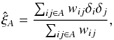 (3)where the wij are weights (Sect. 4.2) and each i or j indexes a measurement on a quasar q at wavelength λ. The sum over (i,j) is understood to run over all pairs of pixels within a bin A in the space of pixel separations, ri − rj. The bins A are defined by a range of width 4 h-1 Mpc of the components perpendicular and parallel to the line of sight, r⊥ and r∥. We used 50 bins in each component, spanning the range from 0 to 200 h-1 Mpc; the total number of bins used for evaluating the correlation function is therefore 2500. Separations in observational pixel coordinates (RA, Dec, z) were transformed into (r⊥,r∥) in units of h-1 Mpc by using the ΛCDM fiducial cosmology described in Table 1.
From sum (3), we excluded pairs of pixels from the same quasar to avoid the correlated errors in δi and δj arising from the estimate of Cq(λ) for the spectrum of the quasar. The weights in Eq. (3) are set to zero for pixels flagged by the pipeline as problematic because of sky emission lines or cosmic rays, for example. Neither did we use pairs of pixels that had nearly the same wavelength (r∥< 4 h-1 Mpc) and that were taken on the same focal-plane plate. The reason for this decision is that these pairs have ~20% greater correlation than expected from our linear cosmological model fit using data with r∥> 4 h-1 Mpc. This result is most likely due to spurious correlations introduced by the pipeline, for instance, from sky subtraction for flux calibration operations.
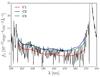 |
Fig. 4 Example of a BOSS quasar spectrum of redshift 2.91 The red and blue lines cover the forest region used here, 104.0 <λrf< 120.0. This region is sandwiched between the quasar’s Lyβ and Lyα emission lines at 400.9 and 475.4 nm The blue (green) line is the C2 (C3) continuum model, Cq(λ), and the red line is the C1 model of the product of the continuum and the mean absorption, |
4.1. Continuum fits
We used three methods to estimate used in Eq. (2). The first two assume that is, to first approximation, the product of two factors: a scaled universal quasar spectrum that is a function of rest-frame wavelength, λrf = λ/ (1 + zq) (for quasar redshift zq), and a mean transmission fraction that slowly varies with absorber redshift. The universal spectrum is found by stacking the appropriately normalized spectra of quasars in our sample, thus averaging the fluctuating Lyα absorption. The continuum for individual quasars is then derived from the universal spectrum by normalizing it to the quasar’s mean forest flux and then modifying its slope to account for spectral-index diversity and/or photo-spectroscopic miscalibration.
Our simplest continuum estimator, C1, is method 1 of Busca et al. (2013). It directly estimates the product in Eq. (2). by modeling each spectrum as 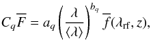 (4)where aq is a normalization, bq a deformation parameter, ⟨ λ ⟩ the mean wavelength in the forest for the quasar q, and
  is the mean normalized flux obtained by stacking spectra in bins of width Δz = 0.1.
As noted in Busca et al. (2013), the mean value of δq(λ) (averaged over all measurements in narrow bins in λ) has peaks at the position of the Balmer series of amplitude ~0.02. These artifacts are due to imperfect use of spectroscopic standards containing those lines. They are removed on average by subtracting the mean δ from each measurement: δq(λ) → δq(λ) − ⟨ δ(λ) ⟩.
The C1 continuum estimator would be close to optimal if the distribution of δ about zero was Gaussian. Since the true distribution is quite asymmetric, we developed a slightly more sophisticated continuum estimator, method 2 of Busca et al. (2013), denoted here as C2. We adopted this as the standard estimator for this work. The continuum for each quasar is assumed to be of the form ![Mathematical equation: \begin{eqnarray} C_q(\lambda)=[a_q + b_q\log(\lambda) ]\overline{C}(\lambda_{\rm rf}) \;, \end{eqnarray}](/articles/aa/full_html/2015/02/aa23969-14/aa23969-14-eq119.png) (5)where
(5)where  is the mean continuum determined by stacking spectra. The parameters aq and bq are fitted to match the quasar’s distribution of transmitted flux to an assumed probability distribution derived from the log-normal model used to generate mock data.
The C2 continuum is then multiplied by the mean transmitted flux fraction , which we determined by requiring that the mean of the delta field vanish for all redshifts. This last step has the effect of removing the average of the Balmer artifacts.
The third continuum-estimating method, C3, is a modified version of the MF-PCA technique described in Lee et al. (2012). This method has been used to provide continua for the publicly available DR9 spectra (Lee et al. 2013). Unlike the other two methods, it does not assume a universal spectral form. Instead, for each spectrum, it fits a variable amplitude PCA template to the part redward of the Lyα wavelength. The predicted spectrum in the forest region is then renormalized so that the mean forest flux matches the mean forest flux at the corresponding redshift.
All three methods use data in the forest region to determine the continuum and therefore necessarily introduce distortions in the flux transmission field and its correlation function (Slosar et al. 2011). Fortunately, these distortions are not expected to shift the BAO peak position, and this expectation is confirmed in the mock spectra.
4.2. Weights
We chose the weights wij so as to approximately minimize the relative error on  estimated with Eq. (3). The weights should obviously favor low-noise pixels and take into account the redshift dependence of the pixel correlations, ξij(z) ∝ (1 + zi)γ/ 2(1 + zj)γ/ 2, with γ ~ 3.8 (McDonald et al. 2006). Following Busca et al. (2013), we used
  (6)where ξii is assumed to have noise and LSS contributions:
 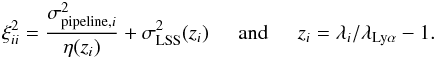 (7)Here
  is the pipeline estimate of the noise-variance of pixel i multiplied by
  , and η is a factor that corrects for a possibly inaccurate estimate of the variance by the pipeline. The two functions η(z) and
  are determined by measuring the variance of δi in bins of and redshift.
4.3. ξ (r⊥, r∥) and its covariance
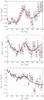 |
Fig. 5 Measured correlation functions (continuum C2) in three angular regions: μ> 0.8 (top), 0.8 >μ> 0.5 (middle), and 0.5 >μ> 0. (bottom), where μ is the central value of |
The correlation function ξ(r⊥,r∥) was measured for the three continuum methods. Figure 5 shows the result using the C2 method, averaged for three ranges of  . (The analogous plots for C1 and C3 are provided in Appendix C.) The superimposed curves present the results of fits as described in Sect. 5. The full curve displays the best fit, while the dashed curves are the fit when the parameters α⊥ and α∥ (Eq. (11)) are set to unity, that is, imposing the BAO peak position of the fiducial cosmology.
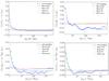 |
Fig. 6 Correlation |
![Mathematical equation: \hbox{$C(\rperp,\rpar,\rperp^\prime,\rpar^\prime)/ [{\rm Var}(\rperp,\rpar) {\rm Var} (\rperp^\prime,\rpar^\prime)]^{1/2}$}](/articles/aa/full_html/2015/02/aa23969-14/aa23969-14-eq140.png)


We evaluated the covariance matrix,  using two methods described in Appendix A. The first uses sub-samples and the second a Wick expansion of the four-point function of the δ field. The two methods give covariances whose differences lead to no significant differences in fits for cosmological parameters. We used the sub-sample covariance matrix in the standard fits.
The 2500 × 2500 element covariance matrix has a relatively simple structure. By far the most important elements are the diagonal elements, which are, to good approximation, inversely proportional to the number of pixel pairs used in calculating the correlation function:  (8)This is about twice the value that one would calculate assuming that all pixel pairs used to calculate ξ(r⊥,r∥) are independent. This decrease in the effective number of pixels is due to the correlations between neighboring pixels on a given quasar: because of these correlations, a measurement of ξ(r⊥,r∥) using a pair of pixels from two quasars is not independent of another measurement of ξ(r⊥,r∥) using the same two quasars.
The off-diagonal elements of the covariance matrix also have a simple structure. The reasons for this structure are made clear by the Wick expansion in Appendix A, which relates the covariance to correlations within pairs-of-pairs of pixels. The strongest correlations are in pairs-of-pairs where both pairs involve the same two quasars. To the extent that two neighboring forests are parallel, these terms contribute only to the covariance matrix elements with  , corresponding to the transverse separation of the forests. The elements of the correlation matrix as a function of
  are illustrated in Fig. 6 (top left); they closely follow the correlation function ξ(Δλ) found within individual forests.
The covariance for  is due to pairs-of-pairs involving three or more quasars and, for small
  , to the fact that neighboring forests are not exactly parallel. As illustrated in Fig. 6, the covariances are rapidly decreasing functions of and
  .
.
The statistical precision of the sub-sampling method is ~0.02 for individual elements of the correlation matrix. We adopted this method for the standard analysis because it is much faster than the more precise Wick method and is therefore better adapted to studies where the data sample and/or analysis protocol is varied. Figure 6 shows that only correlations with Δr⊥ = 0,Δr∥< 20 h-1 Mpc are greater than the statistical precision and therefore sufficiently large for individual matrix elements to be measured accurately by sub-sampling. We therefore used the average correlations as a function of and , ignoring small observed variations with  and
and  . The analysis of the mock spectra (Sect. 5.2) indicates that this procedure is sufficiently accurate to produce reasonable χ2 values and that the distribution of estimated BAO peak positions is similar to that expected from the uncertainties derived from the χ2 surfaces.
5. Fits for the peak position
To determine the position of the BAO peak in the transverse and radial directions, we fit the measured ξ(r⊥,r∥) using the techniques described in Kirkby et al. (2013).
5.1. BAO model
We fit the measured ξ(r∥,r⊥) to a form that includes a cosmological correlation function ξcosmo and a broadband function ξbb that takes into account imperfect knowledge of the non-BAO cosmology and distortions introduced by the analysis:  (9)The function ξcosmo is described as a sum of a non-BAO smooth function and a BAO peak function,
  (10)where apeak controls the amplitude of the BAO peak relative to the smooth contribution. The radial and transverse dilation factors describing the observed peak position relative to the fiducial peak position are
 ![Mathematical equation: \begin{eqnarray} \apar = \frac { \left[D_H(\bar z)/r_{\rm d}\right] }{\left[D_H(\bar z)/r_{\rm d}\right]_{\rm fid}} \hspace*{3mm}{\rm and}\hspace*{5mm} \aperp = \frac { \left[D_{\rm A}(\bar z)/r_{\rm d}\right] }{\left[D_{\rm A}(\bar z)/r_{\rm d}\right]_{\rm fid}}, \label{eq:alpha} \end{eqnarray}](/articles/aa/full_html/2015/02/aa23969-14/aa23969-14-eq166.png) (11)where rd is the sound horizon at the drag epoch (defined to sufficient accuracy for each cosmology by Eq. (55) of Anderson et al. 2014).
(11)where rd is the sound horizon at the drag epoch (defined to sufficient accuracy for each cosmology by Eq. (55) of Anderson et al. 2014).
The function ξcosmo was calculated from the power spectrum using the following procedure. We modeled the Lyα forest power spectrum including redshift-space distortions and nonlinear effects as ![Mathematical equation: \begin{eqnarray} P(k,\mu_{k}) &=& b^{2}(1 + \beta\mu_{k}^{2})^{2} \nonumber\\ &&\times\left[ P_{\rm peak}(k)\exp(-k^{2}\Sigma^{2}(\mu_{k})/2) + P_{\rm smooth}(k)\right], \label{eq:Pk} \end{eqnarray}](/articles/aa/full_html/2015/02/aa23969-14/aa23969-14-eq167.png) (12)where
(12)where  , b is the Lyα forest bias parameter and β is the redshift-space distortion parameter. Here, we defined Ppeak(k) = Plin(k) − Psmooth(k), where Plin is the linear-theory matter power spectrum from CAMB (Lewis et al. 2000) calculated using the cosmological parameters from the first column of Table 1, and Psmooth is the CAMB power spectrum with the BAO feature erased following the method of Kirkby et al. (2013). The exponential function in Eq. (12) models the anisotropic nonlinear broadening from structure growth (Eisenstein et al. 2007) with
  and is only applied to the BAO feature. The default values we adopted are Σ∥ = 6.41 h-1 Mpc and Σ⊥ = 3.26 h-1 Mpc, which are inferred from the amplitude of the variation of linear peculiar velocities along the line of sight that cause a relative displacement of pixel pairs contributing to the BAO peak form (White 2014).
The power spectrum multipoles are given by  (13)where Lℓ is the Legendre polynomial. The corresponding correlation function multipoles are then
  (14)where jℓ is the spherical Bessel function. Finally, the correlation function is the sum of the multipoles
  (15)The nonlinear broadening in principle transfers power to higher even multipoles ℓ = 6,8,..., but the contribution from these higher-order multipoles is negligible.
We wish to ensure the insensitivity of our results to non-BAO cosmology and to inaccurately modeled astrophysical effects such as UV fluctuations, nonlinear effects, and DLAs. We therefore use a broadband function, ξbb to include inaccuracies in the non-BAO correlation function as well as distortions due, for example, to continuum fitting. We used the form  (16)where the L2j is the Legendre polynomial of order 2j. Our standard model uses (imax,jmax) = (2,2).
The standard fits use the fiducial values of Σ⊥ and Σ∥, and set apeak = 1. They thus have four physical free parameters (b,β,α⊥,α∥) and, for the fiducial model, nine broadband distortion parameters. The standard fit uses the range 40 h-1 Mpc <r< 180 h-1 Mpc, giving a total of 1515 bins in (r∥,r⊥) for the correlation function measurements that are actually used in the fit, and 1502 degrees of freedom.
5.2. Fits with the mock data sets
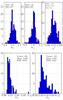 |
Fig. 7 Summary of the results of fits for (α∥, α⊥) for the 100 mock catalogs. The histograms show the best-fit values, the minimum χ2 values and the 1σ uncertainties. |
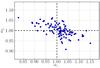 |
Fig. 8 Measured α∥ and α⊥ for the 100 mock catalogs. |
Figure 7 summarizes the results of the cosmological fits on the 100 sets of mock spectra. The mean recovered α∥ and α⊥ are consistent with unity, indicating no bias in the measurement of the BAO peak position3. The numbers of α∥ measurements within 1σ and 2σ of unity are 61 and 93, consistent with the expected numbers, 68 and 95.5. For α⊥ the numbers are 68 and 95. For the combined (α∥,α⊥) measurements, 70 are within the 1σ and 93 within the 2σ contours.
The rms deviations of α∥ and α⊥ are 0.029 and 0.057. The mean χ2 is similar to the number of degrees of freedom, indicating that the model represents the mock observations sufficiently well and that the covariance matrix is well estimated.
Figure 8 shows an anticorrelation between the recovered α∥ and α⊥, with a correlation coefficient of − 0.6. The quantity of the form  with the smallest mock-to-mock variance has w ~ 0.7, with an rms deviation of 0.017. This result is to be compared with the optimal quantity for galaxy surveys, ~
 . The difference arises because redshift distortions are stronger for the Lyα forest, a consequence of the low bias factor that enables more precise measurements in the r∥ direction even though there are two dimensions for r⊥ and only one for r∥. This effect is evident in Fig. 5 where the BAO peak is most easily seen for μ> 0.8.
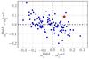 |
Fig. 9 Difference in best-fit α∥ and α⊥ values between high redshift (z> 2.295) and low redshift (z< 2.295) subsets of the 100 mock realizations and the observations (red star). Compared with Fig. 8, the plot shows the degraded precision resulting from dividing the data into two redshift bins. |
Figure 9 presents the results of fits separating the mock data into two redshift bins, z< 2.295 and z> 2.295. The differences between the measured α∥ and α⊥ for the two bins are typically of about 10%.
5.3. Fits with the observations
Results for the standard fit and modified fits.
Table 2 gives the results of fits of the data for a variety of data sets and analysis assumptions. The first line lists our standard analysis using the C2 continua:  (17)The precisions on α∥ and α⊥ inferred from our χ2 fitting procedure are typical of those found using the 100 mock catalogs (Fig. 7). The full contours presented in Fig. 10 show that these errors are somewhat non-Gaussian, with an anti-correlation between α∥ and α⊥. In particular, the 2σ contour extends asymmetrically to large α⊥, consistent with the visual impression from Fig. 5. The most precisely determined combination is
 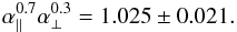 (18)The next seven lines of Table 2 present the results of analyses using the standard data set, but with modified assumptions: using the non-standard continua C1 and C3; adding a Gaussian prior to the redshift distortion parameter around its nominal value β = 1.4 of width 0.4; freeing the peak amplitude apeak; fitting the nonlinearity parameters, Σ∥ and Σ⊥, or setting them to zero (and thus not correcting for nonlinearities); using spectra with one or more DLA, but without a special treatment (fit with Voigt profile). Because these seven fits all use the same data set, any variation of the results at the 1σ level might indicate a systematic effect. In fact, all configurations produce results that are consistent at the sub-σ level. We note, however, that the 1σ precision on α⊥ is degraded through use of C1 and C3, although C1 does almost as well as C2 at the 2σ level. The higher sensitivity of the α⊥ uncertainty to the continuum method compared with that for the α∥ uncertainty might be expected from the low statistical significance of the BAO peak in transverse directions. The central value and error of α∥ are robust to these differences.
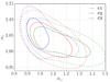 |
Fig. 10 Constraints on (α∥,α⊥) using the three continuum estimators, C1 (red), C2 (blue), and C3 (green). The solid and dashed contours correspond to 1σ and 2σ (Δχ2 = 2.3,6.2). |
The next two lines in Table 2 are the results for C2 with reduced data sets: using a short forest (104.5 <λrf< 118.0 nm) farther away from the Lyα and Lyβ peaks, or removing spectra with one or more DLAs. Both results are consistent at 1σ with those obtained with the more aggressive standard data set but, as expected, with larger statistical errors.
The next two lines present the results obtained by dividing the pixel-pair sample into two redshift bins. The two results now correspond to fairly independent samples and agree at the 2σ level. The differences between measurements of (α∥,α⊥) for the two redshift bins in the mock spectra are displayed in Fig. 9, suggesting that the observed difference is similar to that observed with the mock spectra.
The last line of Table 2 is the χ2 for a fit without a BAO peak. Comparison with the first line reveals Δχ2 = 27.2 for two additional degrees of freedom, corresponding to a 5σ detection.
6. Systematic errors
The uncertainties reported in Table 2 are statistical and are derived from the χ2 surface. In this section we discuss possible systematic errors. We find no evidence for effects that add uncertainties similar to the statistical errors.
We derived cosmological information by comparing the measured flux correlation function with a model, defined by Eqs. (9), (10) and (16), that depends on cosmological parameters (Eq. (10)). Systematic errors in the derived parameters can result if either the assumed model or the measured correlation function differ systematically from the true flux-correlation function.
In fitting the data, we added a general broadband form ξbb (Eq. (16)) to the assumed cosmological correlation function ξcosmo. The role of ξbb is to make the fit sensitive only to the position of the BAO peak and not to the more uncertain smooth component of ξcosmo. To verify that the broadband does indeed remove any sensitivity to smooth components of the correlation function, we varied the form of the assumed broadband and the range over which it was fit. The results, listed in Table 3, show no significant variation of the derived (α∥,α⊥), indicating that the broadband performed as required. Of particular significance, adding greater freedom to ξbb only has an impact of about 10% impact on the size of the α∥ error, although it has a stronger impact (20–30%) on the α⊥ error.
Because the use of ξbb makes our results insensitive to smooth features in ξ, we are primarily concerned with rough effects either due to observing or analysis artifacts or to physical effects that invalidate the assumed theoretical form (Eq. (9)).
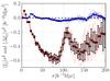 |
Fig. 11 Effect of metals on the measured correlation function for 10 mock sets. The red circles show r2ξ(r) for μ> 0.8 averaged over the 10 mock sets The blue circles show the difference between r2ξ(r) and r2ξ(r) in the same mock realization, but without metals. The light red and blue lines show the results for individual mock sets, the error bars give the standard deviation of the 10 realizations. |
We first considered errors in the theoretical form of the correlation function. The function ξcosmo in (9) is subject to uncertainties arising from nonlinear effects and, more importantly, in the astrophysical processes that determine the flux transmission correlations from matter correlations. The resulting uncertainties in the dominant Lyα absorption would be expected to generate only errors that vary slowly with r and are therefore absorbed into ξbb. On the other hand, absorption by metals, not included in (9), generates an excess correlation in individual forests in the form of narrow peaks centered on the wavelength separations between λLyα and metal lines. For example, the SiII(1260.42) absorption correlated with Lyα (1215.67) absorption gives rise to a narrow peak of excess correlation at r = 110 h-1 Mpc on the line of sight, at z = 2.34. This narrow peak is smeared because of the range of observed redshifts, over a width Δr ~ ± 5 h-1 Mpc. This correlation in the absorption in individual quasar spectra induces a correlation in the spectra of neighboring quasars (small r⊥), because they probe correlated structures of Lyα and SiII absorption in the intergalactic medium.
As described in Bautista et al. (in prep.), we added metals to the mock spectra to estimate their importance. As expected, the mocks indicate that the metal-induced correlation rapidly decreases with transverse separation, dropping by a factor of five between the first and third r⊥ bin. Figure 11 shows the effect on ten sets of mocks in the important region μ> 0.8. The modifications do show structure that might not be modeled by our broadband term. Fortunately, the effect has no significant impact on the measured position of the BAO peak, with (α∥,α⊥) for metaled and metal-free mocks having a mean difference and mock-to-mock dispersion of Δα∥ = 0.002 ± 0.003 and Δα⊥ = 0.003 ± 0.009.
Because the amplitude of the metal lines is somewhat uncertain, we empirically verified that they are unimportant by re-performing the fit of the DR11 data after excising the correlation function bins with  . Most of the metal correlation occurs within r⊥< 10 h-1 Mpc, so any unexpected effect from metal lines would have to be made apparent by a dependence of the BAO results on
  . In fact, the results are remarkably stable, as shown in Fig. 12. We thus conclude that absorption by metals is unlikely to significantly affect the measured position of the BAO peak.
We now examine artifacts introduced by the analysis. The measured correlation function will be different from the true flux-transmission correlation function because of systematic errors in the flux-transmission field, δq(λ), defined by Eq. (2). Such errors can be introduced through an inaccurate flux-calibration or an inaccurate estimate of the function  . These errors in δq(λ) will generate systematic errors in the correlation function if the neighboring quasars have correlated systematic errors.
The most obvious error in the δq(λ) arises from the necessity of using a spectral template to estimate the continuum. The C1 and C2 methods use a unique template that is multiplied by a linear function to fit the observed spectrum. This approach results in two systematic errors on the correlation function. First, as previously noted, fitting a linear function for the continuum effectively removes broadband power in individual spectra. This error will be absorbed into ξbb and not generate biases in the BAO peak position. Second, δq(λ) along individual lines of sight will be incorrect because non-smooth quasar spectral diversity is not taken into account by the universal template. However, because the peculiarities of individual quasar spectra are determined by local effects, they would not be expected to be correlated between neighboring quasars. The tests with the mock catalogs that include uncorrelated spectral diversity confirm that the imprecisions of the continuum estimates do not introduce biases into the estimates of the BAO peak positions.
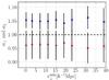 |
Fig. 12 Values α∥ (blue dots) and α⊥ (red dots) recovered from the DR11 data for different choices of the minimum transverse separation, |
Errors introduced by the flux calibration are potentially more dangerous. The BOSS spectrograph (Smee et al. 2013) is calibrated by observing stars whose spectral shape is known. Most of these objects are F-stars whose spectra contain the Balmer series of hydrogen lines. The present BOSS pipeline procedure for calibration imperfectly treats the standard spectra in the neighborhood of the Balmer lines, resulting in calibration vectors, C(λ), that show peaks at the Balmer lines of amplitude ⟨ ΔC/C ⟩ ~ 0.02 ± 0.004, where the ±0.004 refers to our estimated quasar-to-quasars rms variation of the Balmer artifacts (Busca et al. 2013). If uncorrected, these calibration errors would lead to δ ~ 0.02 at absorber redshifts corresponding to the Balmer lines. The subtraction of the mean δ-field, ⟨ δ(λ) ⟩ in our analysis procedure removes this effect on average, but does not correct calibration vectors individually. Because of the relative uniformity of the Balmer feature in the calibration vectors, this mean correction is expected to be sufficient. In particular, we have verified that no significant changes in the correlation function appear when it is calculated taking into account the observed correlations in the Balmer artifacts, ΔC/C.
To verify this conclusion, we searched for Balmer artifacts in the measured ξ(r∥,r⊥, ⟨ λ ⟩) where ⟨ λ ⟩ is the mean wavelength of the pixel pair. If our mean correction is insufficient, there would be excess correlations at r∥ = 0 and ⟨ λ ⟩ equal to a Balmer wavelength. Artifacts would also appear at r∥ and ⟨ λ ⟩ corresponding to pairs of Balmer lines. For example, the pair [Hδ (410 nm), Hϵ (397 nm)] would produce excess correlation at the corresponding radial separation 98 h-1 Mpc and ⟨ λ ⟩ = 403 nm. A search has yielded no significant correlation excesses. Additionally, removing from the analysis pixel pairs near (397, 410) nm, dangerously near the BAO peak, does not generate any measurable change in the BAO peak position.
7. Cosmological implications
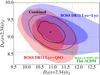 |
Fig. 13 Constraints on (DA/rd,DH/rd). Contours show 68.3% (Δχ2 = 2.3) and 95.5% (Δχ2 = 6.2) contours from the Lyα forest autocorrelation (this work, blue), the quasar Lyα forest cross-correlation (Font-Ribera et al. 2014) (red), and the combined constraints (black). The green contours are CMB constraints calculated using the Planck+WP+SPT+ACT chains (Planck Collaboration XVI 2014) assuming a flat ΛCDM cosmology. |
The standard fit values for (α∥,α⊥) from Table 2 combined with the fiducial values from Table 1 yield the following results: 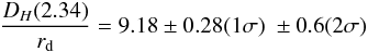 (19)and
 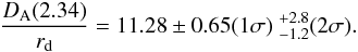 (20)The blue shading in Fig. 13 shows the 68.3% and 95.5% likelihood contours for these parameters, which are mildly anticorrelated. These constraints can be expressed equivalently as
 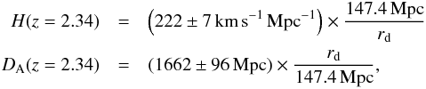 (21)where we have scaled by the value rd = 147.4 Mpc from the Planck+WP model in Table 1.
Our measured values of DH/rd and DA/rd (Eqs. (19) and (20)) can be compared with those predicted by the two CMB inspired flat ΛCDM models from Table 1: (8.570,11.76) for Planck+WP and (8.648,11.47) for WMAP9+ACT+SPT. Figure 13 demonstrates that our values differ by 1.8σ from those of the Planck+WP model. They differ from the WMAP9+ACT+SPT model by 1.6σ. We emphasize that, in contrast to the values of α∥ and α⊥, the constraints quoted in Eq. (19)–(21) are independent of the fiducial model adopted in the analysis, at least over a substantial parameter range. We have confirmed this expectation by repeating some of our analyses using the Planck+WP parameters of Table 1 in place of our standard fiducial model, finding negligible change in the inferred values of DH/rd and DA/rd.
To illustrate this tension, we show in Fig. 14 values of ΩM and ΩΛ that are consistent with our measurements. We consider models of ΛCDM with curvature, having four free parameters: the cosmological constant, the matter and the baryon densities, and the Hubble constant (ΩΛ,ΩM,ΩBh2,h). For clarity, we placed priors on two of them, adopting the Planck value of ΩBh2 (Planck Collaboration XVI 2014) and adopting a wide prior on h = 0.706 ± 0.032 meant to cover the value measured with the local distance ladder (Riess et al. 2011) and that measured with CMB anisotropies assuming a ΛCDM cosmology (Planck Collaboration XVI 2014).
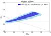 |
Fig. 14 Constraints on the oΛCDM parameters (ΩΛ,ΩM) based on the autocorrelation contours of Fig. 13. The contours show 68.3% and 95.5% confidence levels. The Planck value of ΩBh2 is assumed together with a Gaussian prior for H0 = 70.6 ± 3.2 km s-1 Mpc-1. The yellow star is the Planck ΛCDM measurement, the dashed line corresponds to a flat Universe. |
With these priors, Fig. 14 shows that the flat ΛCDM model preferred by CMB data (Planck Collaboration XVI 2014) lies near the 95.5% confidence level of our measurement. We note that values of (ΩM,ΩΛ) far from the line ΩM + ΩΛ = 1 disagree with the combination of CMB data and BAO at z< 1, which require 1 − ΩM − ΩΛ = −0.0005 ± 0.0066 (Planck Collaboration XVI 2014).
The tension with CMB data is also seen in the BAO measurement using the quasar-Lyα forest cross-correlation (Font-Ribera et al. 2014).
The measurement of this function follows a procedure that is similar to that used here, except that the estimator (3) is replaced with ∑ wiδi/ ∑ wi where the sum is now over forest pixels i separated from any quasar within a range of (r⊥,r∥).
Red contours in Fig. 13 show the 68.3% and 95.5% likelihood contours derived from the cross-correlation. The implied values of DA and DH are consistent between the autocorrelation and cross-correlation measurements, but the statistical errors are interestingly complementary. The autocorrelation constrains DH more tightly than DA because redshift-space distortions are so strong in Lyα forest clustering, a consequence of the low bias factor of the forest. While there are far fewer quasar-forest pairs than forest-forest pairs, the cross-correlation still yields a useful BAO signal because the quasars themselves are highly biased, which boosts the clustering amplitude. However, redshift-space distortions are weaker in the cross-correlation for the same reason, and the cross-correlation analysis yields comparable statistical errors in the transverse and line-of-sight BAO. The cross-correlation constraint therefore suppresses the elongated tails of the autocorrelation likelihood contours seen in Fig. 10 toward high DA and correspondingly low DH.
The statistical errors in these BAO measurements are dominated by combinations of limited sampling of the volume probed, by instrumental noise in the Lyα forest spectra, and (for the cross-correlation measurement) by shot noise of the quasar density field. For this reason, the statistical errors in the two BAO measurements are almost completely uncorrelated, as discussed in detail in Appendix B. We therefore combined the two likelihood surfaces as if they were independent to produce the joint likelihood contours shown by the solid lines in Fig. 13. Marginalized 1D constraints from the combined likelihood are 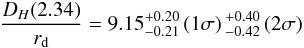 (22)and
 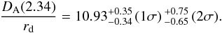 (23)These numbers can be compared with the green contours in Fig. 13, which show the 68.3%, 95.5%, and 99.7% confidence contours on DA/rd and DH/rd derived from CMB data (specifically, using the Planck + WMAP polarization + SPT + ACT chains available from the Planck Collaboration; this data set gives results very similar to the Planck+WP model of Table 1), assuming a flat ΛCDM cosmological model. These predictions lie outside the 95.5% likelihood interval for the combined cross- and autocorrelation BAO measurements, an ≈2.5σ tension with the data. The tension with the WMAP9+ACT+SPT model of Table 1 is slightly smaller, ≈2.2σ. In more detail, the Planck ΛCDM prediction is approximately 2σ below the value of DH inferred from the autocorrelation and approximately 2σ above the value of DA inferred from the cross-correlation, deviations of ≈7% in each case. The tension between the CMB-constrained flat ΛCDM model and the autocorrelation measurement of DH is evident in the top panel of Fig. 5, where the peak in the data is visually to the left of the peak in the fiducial model (and would be even more to the left of the Planck+WP model).
How seriously should one take this tension? For the autocorrelation function, the success of our method in reproducing the correct parameters when averaged over our 100 mock catalogs, and the insensitivity of our derived α∥ and α⊥ to many variations of our analysis procedure as discussed in Sect. 6, both suggest that systematic biases in our measurements should be smaller than our quoted errors. The agreement between the directly estimated statistical errors and the scatter in best-fit α values for our mock catalogs indicate that our error estimates themselves are accurate, although with 100 mock catalogs we cannot test this accuracy stringently. The most significant impact seen with varying the analysis procedure in Sect. 6 is the larger statistical errors on α∥ and α⊥ for the continuum subtraction method C1. Detailed examination of the likelihood contours in Fig. 10 shows that the larger α∥ errors (and lower central value) for the C1 method are a consequence of its weaker constraint on α⊥, which allows contours to stretch into the region of low α∥ and high α⊥. These regions are inconsistent with the stronger α⊥ constraints of the cross-correlation measurement, so in a joint likelihood they would be eliminated in any case. Furthermore, our standard C2 subtraction method is clearly more realistic than the C1 method because it is based on a more realistic flux PDF rather than a Gaussian approximation to it. Nonetheless, the variation seen in Table 2 suggests some degree of caution about the precision of our statistical errors, even though we have no clear evidence that they are underestimated, particularly because of the relatively weak detection of the transverse BAO signal.
We note that while we used mock spectra to verify the statistical errors of the autocorrelation function, this was not possible for the cross-correlation function because we do not have mock spectra with Lyα absorption correlated with quasar positions. We are in the process of producing such mock spectra, and they will be used in future publications.
While it is premature to conclude that a major modification of ΛCDM is needed, it is nevertheless interesting to note what sorts of changes are indicated by the data. The most widely discussed extensions to flat ΛCDM , allowing nonzero space curvature or a dark energy equation-of-state with w ≠ −1, do not readily resolve the difference seen in Fig. 13 without running afoul of other constraints. This is because of the necessity of decreasing DA(2.34) while increasing DH(2.34), which is difficult because the former is related to the integral of the latter.
Requirements for more general forms of dark energy can be found by considering our measurement of H(z), which, combined with the Friedman equation, determines the density of dark energy ρde(z). Assuming space to be flat and matter to be conserved, and neglecting the radiation density, we have  (24)Dividing by ρde(z = 0) gives
  (25)The uncertainty on ρde(z = 2.34) /ρde(0) is dominated by the difference between two nearly equal numbers in the numerator. If we use the precise values of rd and ΩMh2 = 0.143 ± 0.003 from the Planck+WP CMB power spectrum measurement, the uncertainty is dominated by that of our value of rdH(z = 2.34) (Eq. (22)). We find
 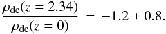 (26)The difference of ~2.5σ from the expected value of unity for the ΛCDM model is the same as the difference discussed above (although the quoted error above implies a 2.8σ deviation, this is reduced slightly by the non-Gaussianity of the likelihood distribution of the measured DH). If a negative value of ρde were to persist as measurement errors on H(z) from BAO and ΩMh2 from the CMB are improved, this would imply that the dark energy density at z = 2.4 is lower than that of z = 0, perhaps even with the opposite sign. This conclusion could be avoided if matter were not conserved from the epoch of recombination, (invalidating the use of the Planck value of ΩMh2 in Eq. (24)), or that the Universe is closed (adding a positive term to the r.h.s. of Eq. (24)). If, in addition to explaining the low value of H(z = 2.34), one wishes to reproduce the low observed value of DA(z = 2.34), there are further constraints on the model. For example, a flat dark-energy model that lowers the value of ρde(z = 2.34) to reproduce the observed H(z = 2.34) would need to increase ρde for 0.7 <z< 2.0 so as to decrease the value of DA(z = 2.34) while maintaining DA(0.57). A compensating decrease of ρde(z> 2.34) would then be needed to maintain the observed value of DA at the last-scattering surface. Detailed discussions of such models will be presented in a forthcoming publication (The BOSS collaboration, in prep.).
8. Conclusions
The Lyα correlation data presented in this study constrain DH/rd and DA/rd at z ~ 2.344. The 3.0% precision on DH/rd and 5.8% precision on DA/rd obtained here improve on the precision of previous measurements: 8% on DH/rd (Busca et al. 2013), and 3.4% on DH/rd and 7.2% on DA/rd (Slosar et al. 2013). The increasing precision of the three studies is primarily due to their increasing statistical power, rather than to methodological improvements. The 2% precision on the optimal combination  can be compared with the 1% precision for DV(z = 0.57) /rd obtained by Anderson et al. (2014).
The derived values of DH/rd and DA/rd obtained here with the Lyα autocorrelation are similar to those inferred from the Quasar-Lyα-forest cross-correlation (Font-Ribera et al. 2014), as shown in Fig. 13. At the two-standard-deviation level, the two techniques are separately compatible with the Planck+WP and fiducial models of Table 1. However, the combined constraints are inconsistent with the Planck+WP ΛCDM model at ≈2.5σ significance, given our estimated statistical uncertainties. The tests presented in earlier sections suggest that our statistical error estimates are accurate and that systematic uncertainties associated with our modeling and analysis procedures are smaller than these statistical errors.
We are in the process of addressing what we consider to be the main weaknesses of our analysis. The artifacts in the spectrophotometric calibration due, for example, to Balmer lines, will be eliminated. More sophisticated continuum modeling making use of spectral features will allow us to verify that unsuspected correlated continua in neighboring quasars are not introducing artifacts in the autocorrelation function. Finally, we are producing realistic mock catalogs with quasar positions correlated with Lyα absorption features in the corresponding forests. Such mocks would allow us to verify the statistical errors for the cross-correlation measurement and to search for unsuspected correlations between the cross- and autocorrelation function measurements. All of these improvements in the analysis procedure will be used for publications using the higher statistical power of the upcoming DR12.
The cosmological implications of our results will be investigated in much greater depth in a forthcoming paper (The BOSS collaboration, in prep.), where we combine the Lyα-forest BAO with the BOSS galaxy BAO results at lower redshift and with CMB and supernova data, which enables interesting constraints on a variety of theoretical models.
Online material
Appendix A: Covariance matrix
Appendix A.1: Estimation of the covariance via a Wick expansion.
The Wick expansion for the covariance between ξ for two bins A and B is the sum over pairs of pairs: ![Mathematical equation: \appendix \setcounter{section}{1} \begin{eqnarray} C_{AB}\; = S_{AB}^{-1} \sum_{i,j\in A} \sum_{k,l\in B} w_i w_j w_k w_l [\xi_{ik}\xi_{jl} + \xi_{il}\xi_{jk}] \end{eqnarray}](/articles/aa/full_html/2015/02/aa23969-14/aa23969-14-eq350.png) (A.1)with
(A.1)with  (A.2)The pairs (i,j) and (k,l) refer to the ends of the vectors rA ∈ A and rB ∈ B. The normalization factor is
 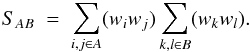 (A.3)As illustrated in Fig. A.1, there are six types of pairs-of-pairs, (ijkl), characterized by the number of distinct points (2, 3, 4) and numbers of quasars (2, 3, 4).
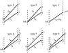 |
Fig. A.1 Six types of pairs of pairs. The dashed lines refer to the quasar lines-of-sight. The variances are dominated by types 1, 2, and 3. The ( |
The complete sum of pairs-of-pairs would require a prohibitively long computer time. We therefore evaluated the sum by using only a random sample of pairs-of-pairs and by replacing products of distinct pixels with the previously evaluated correlation function, either 1D for pairs involving only one quasar, or 3D for pairs involving two quasars
The variances, Eq. (8), are dominated (~97%) by the two-quasar diagrams in Fig. A.1. About 60% of the variance is produced by the diagonal diagram (i = k,j = l). The nondiagonal terms, (i = k,j ≠ l) and (i ≠ k,j ≠ l) account for 25% and 15% of the variance. The dominant covariances, that is, those with and 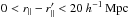 , are dominated by the nondiagonal two-quasar diagrams.
The Wick results for the important covariance matrix elements are summarized in Fig. 6.
Appendix A.2: Estimation of the covariance via sub-sampling
We used a sub-sample method to estimate the covariance matrix. The method consists of organizing the space of pairs of quasars into sub-samples. We took advantage of the fact that quasars are observationally tagged with the number of the plate on which they were observed. A given pair belongs to the sub-sample p if the quasar with the smaller right ascension in the pair was observed at plate p. Thus there are as many sub-samples as the number of plates (Nplates) that compose the data sample (Nplates = 2044 for DR11).
In terms of this partition of the data sample into sub-samples, we write our estimator of the correlation function in Eq. (3) as  (A.4)where
  is the correlation function calculated using only pairs belonging to the sub-sample p and
  is the sum of their weights. The denominator is equal to the sum of weights in A, the normalization in Eq. (3).
Our partitioning scheme ensures that a pair of quasars contributes to one and only one sub-sample. This approach implies that the correlation between  and
and  (with p ≠ p′) is given only by terms of the form T4, T5, and T6. Below we neglect this small correlation.
The covariance matrix is then given by  (A.5)where, as anticipated, we assumed that crossed terms from different plates are zero. The final step is to use the following estimator for the expression in parentheses, the covariance within a plate:
  (A.6)
(A.6)
Appendix B: Combining the results with those of Font-Ribera et al. (2014)
In this appendix we discuss the level of correlation between the BAO measurement presented in this paper and that measured in Font-Ribera et al. (2014) from the cross-correlation of the Lyα forest with the quasar density field, also using the DR11 of BOSS.
If both analyses were limited by cosmic variance, there would be no gain in combining them, since both would be tracing the same underlying density fluctuations. However, as shown in Appendix B of Font-Ribera et al. (2014), cosmic variance is only a minor contribution to the uncertainties in both measurements. The accuracy of the Lyα autocorrelation measurement (presented here) is limited by the aliasing noise (McDonald & Eisenstein 2007; McQuinn & White 2011) and the instrumental noise, while the cross-correlation measurement (Font-Ribera et al. 2014) is also limited by the shot-noise of the quasar field. Since the dominant sources of fluctuation in the two measurements have a completely different nature, the cross covariance should be small.
To better quantify this statement, we calculate the covariance between the two measurements by computing the cross-correlation coefficient between a bin measured in the autocorrelation  and a bin measured in the cross-correlation
  , defined as
  (B.1)where CAA is the variance in the autocorrelation bin A, Caa is the variance in the cross-correlation bin a, and CAa is the covariance between the two bins.
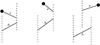 |
Fig. B.1 Three types of diagrams constributing to the covariance between a bin A in the Lyα autocorrelation and a bin a in the cross-correlation with quasars. The dashed lines refer to Lyα forests, the dots to quasars. The solid lines refer to Lyα pixel pairs or quasar-Lyα pairs used to measure the auto- or cross-correlation. |
We calculated the covariance CAa using a Wick expansion similar to that computed in Appendix A. In this case, we must compute a four-point function with three Lyα pixels and a quasar position, and the different contributions to the covariance will be products of the Lyα autocorrelation function between two pixels and the Lyα -quasar cross-correalation between a quasar and a pixel. As shown in Fig. B.1, there will be three types of contribution to the covariance, arising from configurations with two, three, and four quasars.
The correlation of pixels in different lines of sight will in general be weaker than the correlation of pixels in the same line of sight. Therefore, we expect the right-most diagram in Fig. B.1 to have a small contribution, since it involves pixel pairs from different lines of sight.
Direct compuation shows that the contribution from three quasar diagrams is about a factor of ten higher than that from two-quasar diagrams for  . The two-quasar contribution for
  is zero.
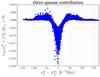 |
Fig. B.2 Cross-correlation coefficients as a function of |
In Fig. B.2 we show the cross-correlation coefficients computed from the three-quasar diagrams as a function of  for
for  (it decreases with increasing
  ). As expected, the correlation between the two measurements is weak, justifying the combined contours presented in Fig. 13.
Appendix C: Correlation function for C1, C2, and C3
Figure C.1 shows the correlation function found using the three continuum estimators in three ranges of μ (the same as those in Fig. 5). All three methods show a clear BAO peak in the nearly radial bin, μ> 0.8. While the peak in this bin is at the same position for all continua, the absolute value of the correlation function is quite different. This is because the μ> 0.8 bin is strongly affected by the distortions induced by the continuum estimator.
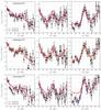 |
Fig. C.1 Measured correlation functions for continuum C1 (top), C2 (middle), and C3 (bottom) averaged over three angular regions: 0 <μ< 0.5 (left), 0.5 <μ< 0.8 (middle), and μ> 0.8 (right), The curves show the results of fits as described in Sect. 5. The blue dashed curves are the best fits, the full red curves are the best fit for C2. |
We follow the convention of Anderson et al. (2014), rd = rs(zd), where rs is the sound horizon and zd is the drag redshift (baryon decoupling from photons), to be distinguished from z∗ (the redshift corresponding to unity optical depth for CMB photons). Earlier publications on BAO generally denoted rd simply as rs. For models with cold dark matter (CDM), baryons and three light neutrino species, rd can be evaluated with Eq. (55) of Anderson et al. (2014), which agrees with the CAMB-derived value to better than 0.1 per cent.
The model has the same ΩMh2, but Ωνh2 = 0. This change has a negligible impact on the generated power spectrum and changes the BAO peak position by only 0.1%.
After we analysed the mocks, we realized that they had been analyzed with a model (the fiducial model of Table 1) that was slightly different from the model used to produce them, which had the same ΩMh2, but Ωνh2 = 0 instead of Ωνh2 = 0.0006. Its value of rd is 0.15 Mpc lower than the fiducial rd, so the expected mean values of α⊥ and α∥ are 0.999, which is sufficiently close to unity for the precision of this study.
The baofit software used in this paper is publicly available at http://github.com/deepzot/baofit/. The measured cross-correlation function and its covariance matrix, and the instructions to reproduce the main BAO results presented in this paper, can be downloaded from http://darkmatter.ps.uci.edu/baofit/, together with the likelihood surfaces used to generate the contours in Fig. 13.
Acknowledgments
Funding for SDSS-III has been provided by the Alfred P. Sloan Foundation, the Participating Institutions, the National Science Foundation, and the US Department of Energy Office of Science. The SDSS-III web site is http://www.sdss3.org/. SDSS-III is managed by the Astrophysical Research Consortium for the Participating Institutions of the SDSS-III Collaboration including the University of Arizona, the Brazilian Participation Group, Brookhaven National Laboratory, Carnegie Mellon University, University of Florida, the French Participation Group, the German Participation Group, Harvard University, the Instituto de Astrofisica de Canarias, the Michigan State/Notre Dame/JINA Participation Group, Johns Hopkins University, Lawrence Berkeley National Laboratory, Max Planck Institute for Astrophysics, Max Planck Institute for Extraterrestrial Physics, New Mexico State University, New York University, Ohio State University, Pennsylvania State University, University of Portsmouth, Princeton University, the Spanish Participation Group, University of Tokyo, University of Utah, Vanderbilt University, University of Virginia, University of Washington, and Yale University. The French Participation Group of SDSS-III was supported by the Agence Nationale de la Recherche under contracts ANR-08-BLAN-0222 and ANR-12-BS05-0015-01. Timothée Delubac and Jean-Paul Kneib acknowledge support from the ERC advanced grant LIDA. Matthew Pieri has received funding from the European Union Seventh Framework Programme (FP7/2007-2013) under grant agreement No. [PIIF-GA-2011-301665]. The authors acknowledge the support of France Grilles for providing computing resources on the French National Grid Infrastructure.
References
- Ahn, C. P., Alexandroff, R., Allen de Prieto, C., et al. 2012, ApJS, 203, 21 [NASA ADS] [CrossRef] [Google Scholar]
- Ahn, C. P., Alexandroff, R., Allen de Prieto, C., et al. 2014, ApJS, 211, 17 [NASA ADS] [CrossRef] [Google Scholar]
- Anderson, L., Aubourg, E., Bailey, S., et al. 2012, MNRAS, 427, 3435 [Google Scholar]
- Anderson, L., Aubourg, E., Bailey, S., et al. 2014, MNRAS, 439, 83 [NASA ADS] [CrossRef] [Google Scholar]
- Becker, R. H., White, R. L., & Helfand, D. J. 1995, ApJ, 450, 559 [NASA ADS] [CrossRef] [Google Scholar]
- Beutler, F., Blake, C., Colless, M., et al. 2011, MNRAS, 416, 3017 [NASA ADS] [CrossRef] [Google Scholar]
- Blake, C., Davis, T., Parkinson, D., et al. 2011, MNRAS, 415, 2892 [NASA ADS] [CrossRef] [Google Scholar]
- Bolton, A., Schlegel, D. J., Aubourg, E., et al. 2012, AJ, 144, 144 [NASA ADS] [CrossRef] [Google Scholar]
- Bovy, J., Hennawi, J. F., Hogg, D. W., et al. 2011, ApJ, 729, 141 [NASA ADS] [CrossRef] [Google Scholar]
- Bovy, J., Myers, A. D., Hennawi, J. F., et al. 2012, ApJ, 749, 41 [NASA ADS] [CrossRef] [Google Scholar]
- Busca, N. G., Delubac, T., Rich, J., et al. 2013, A&A, 552, A96 [NASA ADS] [CrossRef] [EDP Sciences] [Google Scholar]
- Calabrese, E., Hlozek, R. A., Battaglia, N., et al. 2013, Phys. Rev. D, 87, 3012 [Google Scholar]
- Chuang, C.-H., & Wang, Y. 2012, MNRAS, 426, 226 [NASA ADS] [CrossRef] [Google Scholar]
- Cole, S., Percival, W. J., Peacock, J. A., et al. 2005, MNRAS, 362, 505 [NASA ADS] [CrossRef] [Google Scholar]
- Dawson, K., Schlegel, D., Ahn, C., et al. 2013, AJ, 145, 10 [Google Scholar]
- Eisenstein, D. J., Zehavi, I., Hogg, D. W., et al. 2005, ApJ, 633, 560 [NASA ADS] [CrossRef] [Google Scholar]
- Eisenstein, D. J., Seo, H. J., Sirko, E., et al. 2007, ApJ, 664, 675 [Google Scholar]
- Eisenstein, D. J., Weinberg, D. H., Agol, E., et al. 2011, AJ, 142, 72 [Google Scholar]
- Font-Ribera, A., & Miralda-Escudé, J. 2012a, J. Cosmol. Astropart. Phys., 07, 028 [NASA ADS] [CrossRef] [Google Scholar]
- Font-Ribera, A., McDonald, P., & Miral da Escudé, J. 2012b, J. Cosmol. Astropart. Phys., 01, 001 [NASA ADS] [CrossRef] [Google Scholar]
- Font-Ribera, A., Kirkby, D., Busca, N., et al. 2014, J. Cosmol. Astropart. Phys., 05, 027 [NASA ADS] [CrossRef] [Google Scholar]
- Fukugita, M., Ichikawa, T., Gunn, J. E., et al. 1996, AJ, 111, 1748 [NASA ADS] [CrossRef] [Google Scholar]
- Gunn, J. E., Siegmund, W. A., Mannery, E. J., et al. 2006, AJ, 131, 2332 [NASA ADS] [CrossRef] [Google Scholar]
- Hamilton, A. J. S. 1992, ApJ, 385, L5 [NASA ADS] [CrossRef] [Google Scholar]
- Eyal, A., Kazin, E. A., Sanchez, A. G., Cuesta, A. J., et al. 2013, MNRAS, 435, 64 [NASA ADS] [CrossRef] [Google Scholar]
- Kirkby, D., Margala, D., Slosar, A., et al. 2013, J. Cosmol. Astropart. Phys., 03, 024 [NASA ADS] [CrossRef] [Google Scholar]
- Kirkpatrick, J. A., Schlegel, D. J., Ross, N. P., et al. 2011, AJ, 743, 125 [Google Scholar]
- Lawrence, A., Warren, S. J., Almaini, O., et al. 2007, MNRAS, 379, 1599 [NASA ADS] [CrossRef] [MathSciNet] [Google Scholar]
- Lee, K. G., Suzuki, N., & Spergel, D. N. 2012, AJ, 143, 51 [NASA ADS] [CrossRef] [Google Scholar]
- Lee, K. G., Bailey, S., Bartsch, L. E., et al. 2013, ApJ, 145, 69 [Google Scholar]
- Lewis, A., Challinor, A., & Lasenby, A. 2000, ApJ, 538, 473 [NASA ADS] [CrossRef] [Google Scholar]
- Martin, D. C., Fanson, J., Schiminovich, D., et al. 2005, ApJ, 619, L1 [Google Scholar]
- McDonald, P. 2003, ApJ, 585, 34 [NASA ADS] [CrossRef] [Google Scholar]
- McDonald, P., & Eisenstein, D. 2007, Phys. Rev. D, 76, 3009 [Google Scholar]
- McDonald, P., Seljak, U., Schlegel, D. J., et al. 2006, ApJS, 163, 80 [NASA ADS] [CrossRef] [Google Scholar]
- McQuinn, M., & White, M. 2011, MNRAS, 415, 2257 [NASA ADS] [CrossRef] [Google Scholar]
- Mehta, K. T., Cuesta, A., Xu, X., et al. 2012, MNRAS, 427, 2168 [NASA ADS] [CrossRef] [Google Scholar]
- Noterdaeme, P., Petitjean, P., Carithers, W. C., et al. 2012, A&A, 547, L1 [NASA ADS] [CrossRef] [EDP Sciences] [Google Scholar]
- Padmanabhan, N., White, M., & Cohn, J. D. 2009, Phys. Rev. D, 79, 3523 [CrossRef] [Google Scholar]
- Padmanabhan, N., Xu, X., Eisenstein, D. J., et al. 2012, MNRAS, 427, 2132 [NASA ADS] [CrossRef] [MathSciNet] [Google Scholar]
- Palanque-Delabrouille, N., Yèche, C., Myers, A. D., et al. 2011, A&A, 530, A122 [NASA ADS] [CrossRef] [EDP Sciences] [Google Scholar]
- Pâris, I., Petitjean, P., Aubourg, E., et al. 2012, A&A, 548, A66 [NASA ADS] [CrossRef] [EDP Sciences] [Google Scholar]
- Pâris, I., Petitjean, P., Aubourg, E., et al. 2014, A&A, 563, A54 [NASA ADS] [CrossRef] [EDP Sciences] [Google Scholar]
- Percival, W. J., Reid, B. A., Eisenstein, D. J., et al. 2010, MNRAS, 401, 2148 [NASA ADS] [CrossRef] [Google Scholar]
- Pieri, M. M., Frank, S., Weinberg, D. H., Mathur, S., & York, D. G., 2010, ApJ, 724, L73 [Google Scholar]
- Pieri, M. M., Mortonson, M. J., Frank, S., et al. 2014, MNRAS, 441, 1718 [NASA ADS] [CrossRef] [Google Scholar]
- Planck Collaboration XVI. 2014, A&A, 571, A16 [NASA ADS] [CrossRef] [EDP Sciences] [Google Scholar]
- Richards, G. T., Myers, A. D., Gray, A. G., et al. 2009, ApJS, 180, 67 [NASA ADS] [CrossRef] [Google Scholar]
- Riess, A. G., Macri, L., Casertano, S., et al. 2011, ApJ, 730, 119 [NASA ADS] [CrossRef] [Google Scholar]
- Ross, N. P., Myers, A. D., Sheldon, E. S., et al. 2012, ApJS, 199, 3 [NASA ADS] [CrossRef] [Google Scholar]
- Seo, H.-J., Ho, S., White, M., et al. 2012, ApJ, 761, 13 [NASA ADS] [CrossRef] [Google Scholar]
- Slosar, A., Font-Ribera, A., Pieri, M. M., et al. 2011, J. Cosmol. Astropart. Phys., 09, 001 [Google Scholar]
- Slosar, A, Irsic, V., Kirkby, D., et al. 2013, J. Cosmol. Astropart. Phys., 04, 026 [Google Scholar]
- Smee, S., Gunn, J. E., Uomoto, A., et al. 2013, AJ, 146, 32 [Google Scholar]
- Suzuki, N. 2006, ApJS, 163, 110 [NASA ADS] [CrossRef] [Google Scholar]
- Suzuki, N., Tytler, D., Kirkman, D., et al. 2005, ApJ, 618, 592 [NASA ADS] [CrossRef] [Google Scholar]
- Veropalumbo, A., Marulli, F., Moscardini, L., et al. 2014, MNRAS, 442, 3275 [NASA ADS] [CrossRef] [Google Scholar]
- White, M. 2003, The Davis Meeting On Cosmic Inflation, 2003 March 22–25, Davis CA., 18 [Google Scholar]
- White, M. 2014, MNRAS, 439, 3630 [NASA ADS] [CrossRef] [Google Scholar]
- Xu, X., Cuesta, A. J., Padmanabhan, N., et al. 2013, MNRAS, 431, 2834 [NASA ADS] [CrossRef] [Google Scholar]
- Yèche, C., Petitjean, P., Rich, J., et al. 2009, A&A, 523, 14 [Google Scholar]
- York, D. G., Adelman, J., Anderson, J. E., et al. 2000, AJ, 120, 1579 [Google Scholar]
All Tables
Parameters of the fiducial flat ΛCDM cosmological model used for this analysis, the flat ΛCDM model derived from Planck and low-ℓ WMAP polarization data, “Planck + WP” (Planck Collaboration XVI 2014), and a flat ΛCDM model derived from the WMAP, ACT, and SPT data (Calabrese et al. 2013).
All Figures
|
Fig. 1 Hammer-Aitoff projection of the BOSS DR11 footprint (Dec vs. RA). The light areas show the DR9 subregion available for the earlier studies of Busca et al. (2013) and Slosar et al. (2013). The red-dashed line shows the location of the galactic plane. |
| In the text | |
|
Fig. 2 Top: redshift distribution of pixel pairs contributing to ξ in the region 80 <r< 120 h-1 Mpc. Bottom: distribution of all pixel redshifts. |
| In the text | |
|
Fig. 3 Measured correlation function averaged over three angular regions: μ> 0.8 (top), 0.8 >μ> 0.5 (middle), and 0.5 >μ> 0.0 (bottom), where μ is the central value of |
| In the text | |
|
Fig. 4 Example of a BOSS quasar spectrum of redshift 2.91 The red and blue lines cover the forest region used here, 104.0 <λrf< 120.0. This region is sandwiched between the quasar’s Lyβ and Lyα emission lines at 400.9 and 475.4 nm The blue (green) line is the C2 (C3) continuum model, Cq(λ), and the red line is the C1 model of the product of the continuum and the mean absorption, |
| In the text | |
|
Fig. 5 Measured correlation functions (continuum C2) in three angular regions: μ> 0.8 (top), 0.8 >μ> 0.5 (middle), and 0.5 >μ> 0. (bottom), where μ is the central value of |
| In the text | |
|
Fig. 6 Correlation |
| In the text | |
|
Fig. 7 Summary of the results of fits for (α∥, α⊥) for the 100 mock catalogs. The histograms show the best-fit values, the minimum χ2 values and the 1σ uncertainties. |
| In the text | |
|
Fig. 8 Measured α∥ and α⊥ for the 100 mock catalogs. |
| In the text | |
|
Fig. 9 Difference in best-fit α∥ and α⊥ values between high redshift (z> 2.295) and low redshift (z< 2.295) subsets of the 100 mock realizations and the observations (red star). Compared with Fig. 8, the plot shows the degraded precision resulting from dividing the data into two redshift bins. |
| In the text | |
|
Fig. 10 Constraints on (α∥,α⊥) using the three continuum estimators, C1 (red), C2 (blue), and C3 (green). The solid and dashed contours correspond to 1σ and 2σ (Δχ2 = 2.3,6.2). |
| In the text | |
|
Fig. 11 Effect of metals on the measured correlation function for 10 mock sets. The red circles show r2ξ(r) for μ> 0.8 averaged over the 10 mock sets The blue circles show the difference between r2ξ(r) and r2ξ(r) in the same mock realization, but without metals. The light red and blue lines show the results for individual mock sets, the error bars give the standard deviation of the 10 realizations. |
| In the text | |
|
Fig. 12 Values α∥ (blue dots) and α⊥ (red dots) recovered from the DR11 data for different choices of the minimum transverse separation, |
| In the text | |
|
Fig. 13 Constraints on (DA/rd,DH/rd). Contours show 68.3% (Δχ2 = 2.3) and 95.5% (Δχ2 = 6.2) contours from the Lyα forest autocorrelation (this work, blue), the quasar Lyα forest cross-correlation (Font-Ribera et al. 2014) (red), and the combined constraints (black). The green contours are CMB constraints calculated using the Planck+WP+SPT+ACT chains (Planck Collaboration XVI 2014) assuming a flat ΛCDM cosmology. |
| In the text | |
|
Fig. 14 Constraints on the oΛCDM parameters (ΩΛ,ΩM) based on the autocorrelation contours of Fig. 13. The contours show 68.3% and 95.5% confidence levels. The Planck value of ΩBh2 is assumed together with a Gaussian prior for H0 = 70.6 ± 3.2 km s-1 Mpc-1. The yellow star is the Planck ΛCDM measurement, the dashed line corresponds to a flat Universe. |
| In the text | |
|
Fig. A.1 Six types of pairs of pairs. The dashed lines refer to the quasar lines-of-sight. The variances are dominated by types 1, 2, and 3. The ( |
| In the text | |
|
Fig. B.1 Three types of diagrams constributing to the covariance between a bin A in the Lyα autocorrelation and a bin a in the cross-correlation with quasars. The dashed lines refer to Lyα forests, the dots to quasars. The solid lines refer to Lyα pixel pairs or quasar-Lyα pairs used to measure the auto- or cross-correlation. |
| In the text | |
|
Fig. B.2 Cross-correlation coefficients as a function of |
| In the text | |
|
Fig. C.1 Measured correlation functions for continuum C1 (top), C2 (middle), and C3 (bottom) averaged over three angular regions: 0 <μ< 0.5 (left), 0.5 <μ< 0.8 (middle), and μ> 0.8 (right), The curves show the results of fits as described in Sect. 5. The blue dashed curves are the best fits, the full red curves are the best fit for C2. |
| In the text | |
Current usage metrics show cumulative count of Article Views (full-text article views including HTML views, PDF and ePub downloads, according to the available data) and Abstracts Views on Vision4Press platform.
Data correspond to usage on the plateform after 2015. The current usage metrics is available 48-96 hours after online publication and is updated daily on week days.
Initial download of the metrics may take a while.