| Issue |
A&A
Volume 574, February 2015
|
|
|---|---|---|
| Article Number | A59 | |
| Number of page(s) | 17 | |
| Section | Cosmology (including clusters of galaxies) | |
| DOI | https://doi.org/10.1051/0004-6361/201423969 | |
| Published online | 26 January 2015 | |
Online material
Appendix A: Covariance matrix
Appendix A.1: Estimation of the covariance via a Wick expansion.
The Wick expansion for the covariance between ξ for two bins A and B is the sum over pairs of pairs: 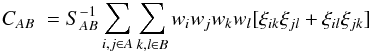 (A.1)with
 ![]() (A.2)The pairs (i,j) and (k,l) refer to the ends of the vectors rA ∈ A and rB ∈ B. The normalization factor is
(A.2)The pairs (i,j) and (k,l) refer to the ends of the vectors rA ∈ A and rB ∈ B. The normalization factor is 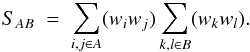 (A.3)As illustrated in Fig. A.1, there are six types of pairs-of-pairs, (ijkl), characterized by the number of distinct points (2, 3, 4) and numbers of quasars (2, 3, 4).
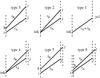 |
Fig. A.1
Six types of pairs of pairs. The dashed lines refer to the quasar lines-of-sight. The variances are dominated by types 1, 2, and 3. The ( |
| Open with DEXTER | |
The complete sum of pairs-of-pairs would require a prohibitively long computer time. We therefore evaluated the sum by using only a random sample of pairs-of-pairs and by replacing products of distinct pixels with the previously evaluated correlation function, either 1D for pairs involving only one quasar, or 3D for pairs involving two quasars
The variances, Eq. (8), are dominated (~97%) by the two-quasar diagrams in Fig. A.1. About 60% of the variance is produced by the diagonal diagram (i = k,j = l). The nondiagonal terms, (i = k,j ≠ l) and (i ≠ k,j ≠ l) account for 25% and 15% of the variance. The dominant covariances, that is, those with ![]() and
and ![]() , are dominated by the nondiagonal two-quasar diagrams.
, are dominated by the nondiagonal two-quasar diagrams.
The Wick results for the important covariance matrix elements are summarized in Fig. 6.
Appendix A.2: Estimation of the covariance via sub-sampling
We used a sub-sample method to estimate the covariance matrix. The method consists of organizing the space of pairs of quasars into sub-samples. We took advantage of the fact that quasars are observationally tagged with the number of the plate on which they were observed. A given pair belongs to the sub-sample p if the quasar with the smaller right ascension in the pair was observed at plate p. Thus there are as many sub-samples as the number of plates (Nplates) that compose the data sample (Nplates = 2044 for DR11).
In terms of this partition of the data sample into sub-samples, we write our estimator of the correlation function in Eq. (3) as 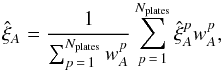 (A.4)where
 ![]() is the correlation function calculated using only pairs belonging to the sub-sample p and
is the correlation function calculated using only pairs belonging to the sub-sample p and ![]() is the sum of their weights. The denominator is equal to the sum of weights in A, the normalization in Eq. (3).
is the sum of their weights. The denominator is equal to the sum of weights in A, the normalization in Eq. (3).
Our partitioning scheme ensures that a pair of quasars contributes to one and only one sub-sample. This approach implies that the correlation between ![]() and
and ![]() (with p ≠ p′) is given only by terms of the form T4, T5, and T6. Below we neglect this small correlation.
(with p ≠ p′) is given only by terms of the form T4, T5, and T6. Below we neglect this small correlation.
The covariance matrix is then given by 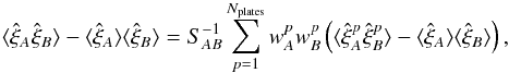 (A.5)where, as anticipated, we assumed that crossed terms from different plates are zero. The final step is to use the following estimator for the expression in parentheses, the covariance within a plate:
 ![]() (A.6)
(A.6)
Appendix B: Combining the results with those of Font-Ribera et al. (2014)
In this appendix we discuss the level of correlation between the BAO measurement presented in this paper and that measured in Font-Ribera et al. (2014) from the cross-correlation of the Lyα forest with the quasar density field, also using the DR11 of BOSS.
If both analyses were limited by cosmic variance, there would be no gain in combining them, since both would be tracing the same underlying density fluctuations. However, as shown in Appendix B of Font-Ribera et al. (2014), cosmic variance is only a minor contribution to the uncertainties in both measurements. The accuracy of the Lyα autocorrelation measurement (presented here) is limited by the aliasing noise (McDonald & Eisenstein 2007; McQuinn & White 2011) and the instrumental noise, while the cross-correlation measurement (Font-Ribera et al. 2014) is also limited by the shot-noise of the quasar field. Since the dominant sources of fluctuation in the two measurements have a completely different nature, the cross covariance should be small.
To better quantify this statement, we calculate the covariance between the two measurements by computing the cross-correlation coefficient between a bin measured in the autocorrelation ![]() and a bin measured in the cross-correlation
and a bin measured in the cross-correlation ![]() , defined as
, defined as 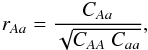 (B.1)where CAA is the variance in the autocorrelation bin A, Caa is the variance in the cross-correlation bin a, and CAa is the covariance between the two bins.
|
Fig. B.1
Three types of diagrams constributing to the covariance between a bin A in the Lyα autocorrelation and a bin a in the cross-correlation with quasars. The dashed lines refer to Lyα forests, the dots to quasars. The solid lines refer to Lyα pixel pairs or quasar-Lyα pairs used to measure the auto- or cross-correlation. |
|
| Open with DEXTER | |
We calculated the covariance CAa using a Wick expansion similar to that computed in Appendix A. In this case, we must compute a four-point function with three Lyα pixels and a quasar position, and the different contributions to the covariance will be products of the Lyα autocorrelation function between two pixels and the Lyα -quasar cross-correalation between a quasar and a pixel. As shown in Fig. B.1, there will be three types of contribution to the covariance, arising from configurations with two, three, and four quasars.
The correlation of pixels in different lines of sight will in general be weaker than the correlation of pixels in the same line of sight. Therefore, we expect the right-most diagram in Fig. B.1 to have a small contribution, since it involves pixel pairs from different lines of sight.
Direct compuation shows that the contribution from three quasar diagrams is about a factor of ten higher than that from two-quasar diagrams for ![]() . The two-quasar contribution for
. The two-quasar contribution for ![]() is zero.
is zero.
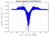 |
Fig. B.2
Cross-correlation coefficients as a function of |
| Open with DEXTER | |
In Fig. B.2 we show the cross-correlation coefficients computed from the three-quasar diagrams as a function of ![]() for
for ![]() (it decreases with increasing
(it decreases with increasing ![]() ). As expected, the correlation between the two measurements is weak, justifying the combined contours presented in Fig. 13.
). As expected, the correlation between the two measurements is weak, justifying the combined contours presented in Fig. 13.
Appendix C: Correlation function for C1, C2, and C3
Figure C.1 shows the correlation function found using the three continuum estimators in three ranges of μ (the same as those in Fig. 5). All three methods show a clear BAO peak in the nearly radial bin, μ> 0.8. While the peak in this bin is at the same position for all continua, the absolute value of the correlation function is quite different. This is because the μ> 0.8 bin is strongly affected by the distortions induced by the continuum estimator.
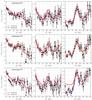 |
Fig. C.1
Measured correlation functions for continuum C1 (top), C2 (middle), and C3 (bottom) averaged over three angular regions: 0 <μ< 0.5 (left), 0.5 <μ< 0.8 (middle), and μ> 0.8 (right), The curves show the results of fits as described in Sect. 5. The blue dashed curves are the best fits, the full red curves are the best fit for C2. |
| Open with DEXTER | |
© ESO, 2015
Current usage metrics show cumulative count of Article Views (full-text article views including HTML views, PDF and ePub downloads, according to the available data) and Abstracts Views on Vision4Press platform.
Data correspond to usage on the plateform after 2015. The current usage metrics is available 48-96 hours after online publication and is updated daily on week days.
Initial download of the metrics may take a while.