| Issue |
A&A
Volume 569, September 2014
|
|
|---|---|---|
| Article Number | A37 | |
| Number of page(s) | 20 | |
| Section | Extragalactic astronomy | |
| DOI | https://doi.org/10.1051/0004-6361/201424217 | |
| Published online | 17 September 2014 | |
Triggering active galactic nuclei in hierarchical galaxy formation: disk instability vs. interactions⋆
INAF – Osservatorio Astronomico di Roma, via di Frascati 33,
00040
Monte Porzio Catone,
Italy
e-mail:
This email address is being protected from spambots. You need JavaScript enabled to view it.
Received:
15
May
2014
Accepted:
23
June
2014
Abstract
Using a state-of-the-art semi analytic model for galaxy formation, we investigated in detail the effects of black hole (BH) accretion triggered by disk instabilities (DI) in isolated galaxies on the evolution of the AGN population. Specifically, we took on, developed, and expanded the Hopkins & Quataert (2011, MNRAS, 411, 1027) model for the mass inflow following disk perturbations, based on a physical description of nuclear inflows and tested against aimed N-body simulations. We compared the evolution of AGN due to such a DI accretion mode with that arising in a scenario where galaxy interactions (IT mode) produce the sudden destabilization of large quantities of gas feeding the AGN; this constitutes the standard AGN feeding mode implemented in the earliest versions of most semi-analytic models. To study the maximal contribution of DI to the evolution of the AGN population, we extended and developed the DI model to assess the effects of changing the assumed disk surface density profile, and to obtain lower limits for the nuclear star formation rates associated to the DI accretion mode. We obtained the following results: i) For AGN with luminosity M1450 ≳ − 26, the DI mode can provide the BH accretion needed to match the observed AGN luminosity functions up to z ≈ 4.5. In such a luminosity range and redshift, it constitutes a viable candidate mechanism to fuel AGN, and can compete with the IT scenario as the main driver of cosmological evolution of the AGN population. ii) The DI scenario cannot provide the observed abundance of high-luminosity QSO with M1450 ≤ −26 AGN, as well as the abundance of high-redhshift z ≳ 4.5 QSO with M1450 ≤ −24. As found in our earliest works, the IT scenario provides an acceptable match to the observed luminosity functions up to z ≈ 6. iii) The dispersion of the distributions of Eddington ratio λ for low- and intermediate-luminosity AGN (bolometric LAGN = 1043−1045 erg s-1) is predicted to be much smaller in the DI scenario compared to the IT mode. iv) The above conclusions concerning the DI mode are robust with respect to the explored variants of the DI model. We discuss the physical origin of our findings. Finally, we discuss how it is possible to pin down the dominant fueling mechanism of AGN in the low-intermediate luminosity range M1450 ≳ −26 where the DI and the IT modes are both viable candidates as the main drivers of the AGN evolution. We show that an interesting discriminant could be provided by the fraction of AGN with high Eddington ratios λ ≥ 0.5, since it increases with luminosity in the IT case, while the opposite is true in the DI scenario.
Key words: galaxies: formation / galaxies: active / galaxies: evolution / galaxies: interactions
Appendices are available in electronic form at http://www.aanda.org
© ESO, 2014
1. Introduction
Understanding the processes driving the growth and evolution of the supermassive black holes (BHs) constitutes a major goal in astrophysics. At the beginning of the past decade, it became widely accepted that the such an evolution is strongly correlated with that of the host galaxies, owing to the observed tightness of the relations between the BH mass and the galaxy properties, such as the stellar mass or the velocity dispersion of the bulge (Kormendy & Richstone 1995; Magorrian et al. 1998, Ferrarese & Merritt 2000; Gebhardt et al. 2000; Marconi & Hunt 2003; Häring & Rix 2004; Aller & Richstone 2007). Together with the observed low fraction of active galactic nuclei (AGN) and with the strong cosmological evolution of the number density of bright AGNs (see, e.g., Richards et al. 2006; Croom et al. 2009; Ueda et al. 2014; for a review see Merloni & Heinz 2013), these measured relations strongly indicated that a major fraction of the BH mass results from accretion of gas during relatively short (duration τ ≈ 107 yrs) but intense (accretion rates Ṁc ≈ 1−10 M⊙/yr), repeated bursts (see, e.g., Shankar et al. 2009; Fiore et al. 2012).
Given this framework, the focus has progressively shifted towards understanding the triggering mechanisms responsible for such intense and short accretion episodes in the galaxy nuclei, and on their relation with the cosmological evolution of galaxies. However, connecting the nuclear accretion with the large-scale properties of galaxies is not an easy task: even the matter located at a radius of a few hundred pc from the central BH must lose more than 99.99% of its angular momentum to be effectively accreted. Numerical simulations on galactic scales have shown that gravitational torques induced by mergers (Hernquist 1989; Barnes & Hernquist 1991; 1996; Heller & Shlosman 1994) or instabilities in self-gravitating disks (Hernquist & Mihos 1995; Bournaud et al. 2005; Eliche-Moral et al. 2008; Younger et al. 2008) – especially in gas rich, high-redshift galaxies (Bournaud et al. 2007; Genzel et al. 2008) – are effective in causing gas inflow down to scales ≲1 kpc. However, both theoretical arguments (Schwarz 1984; Combes & Gerin 1985; Shlosman et al. 1989; Athanassoula 1992) and observational results (see Jogee 2006 for a review) strongly indicate that the transport of gas from galactic scales down to the pc scale (where the BH gravity dominates) requires additional physics.
Again, both external and internal triggers may be effective in providing additional loss of angular momentum. In the case of major mergers, as violent relaxation starts, the gas experiences rapidly varying gravitational torques and suffers strong shocks which can effectively result in large gas inflows in the central region (see Hopkins et al. 2010 and references therein). In the case of isolated galaxies, recent simulations show that – as the disky material at smaller radii becomes self-gravitating – the large-scale bars might indeed trigger a cascade of secondary gravitational instabilities that transport the gas towards the centre (Hopkins & Quataert 2010); the latter process resembles the “bars within bar” scenario (see Shlosman et al. 1989; Friedli & Martinet 1993; Heller & Shlosman 1994; Maciejewski & Sparke 2000) but includes a wider range of morphologies in the nuclear region.
Assessing the role of such processes in determining the cosmological co-evolution of AGN and galaxies is a challenging task. On the observational side, the situation is complex. On the one hand, a correlation between strong galaxy interactions and the AGN activity is found in very luminous QSOs with high mass-accretion rates ≳10 M⊙ yr-1 (Disney et al. 1995; Bahcall et al. 1997; Kirhakos et al. 1999; Hutchings 1987; Yates et al. 1989; Villar-Martin 2011, 2012; Treister et al. 2012). Recently, a clear statistical increase in the AGN fraction in close pairs of galaxies has been found by Ellison et al. (2011), while minor mergers as triggers for lower luminosity AGNs has been proposed to explain the observational features in some nearby galaxies (see, e.g., Combes et al. 2009). The discovery of double AGNs (e.g., Hennawi et al. 2010; McGurk et al. 2011) adds support to a merger origin of the AGN activity. On the other hand, various observational studies suggest that moderately luminous AGN are typically not major-merger-driven at z ≲ 1 (Salucci et al. 1999; Grogin et al. 2005; Pierce et al. 2007; Georgakakis et al. 2009; Cisternas et al. 2011; Villforth et al. 2014), and interestingly also at z ≈ 2 (Rosario et al. 2013a; Silverman et al. 2011; Kocevski et al. 2012). Bournaud et al. (2012) find a correlation between the presence of violent instabilities and AGN activity in gas-rich galaxies at high redshift, thanks to the presence of giant clumps of gas in the disk.
On the theoretical side, aimed, high-resolution N-body simulations can study specific galaxy systems, but understanding the relative effects of the disk instability (DI) and of the galaxy interactions (IT thereafter) as AGN feeding modes requires implementing the physics of nuclear gas inflows into cosmological models of galaxy formation. In turn, this requires an analytical description of such processes to be implemented into existing semi-analytic models (see Baugh 2006 for an introduction) or as sub-grid physics in cosmological simulations. As for the IT scenario, multi-scale high-resolution hydrodynamical N-body simulations are now resolving scales ~10 pc, showing that collisions efficiently cause most of the gas to flow to the centre on timescales of a few dynamical times (see Hopkins et al. 2010 and references therein); analytical – though simplified – or phenomenological descriptions of the inflow determined by mergers have been developed by several authors (see, e.g., Makino & Hut 1997; Cavaliere & Vittorini 2000) and then calibrated and tested against binary hydrodynamic merger simulations (Robertson et al. 2006a,b; Cox et al. 2006; Hopkins et al. 2007b); here the fraction of galactic gas which is able to lose angular momentum and flow to the centre is related to large relative variations Δj/j of the gas specific angular momentum induced by the interactions, which is in turn connected to the mass ratio M′/M of the merging partners.
A different situation holds for the DI scenario. Until recently, no analytic theory that accurately predicts the inflow rates of gas in mixed stellar-plus-gas systems has been worked out; most of the existing works have been based on the over-simplified assumption of completely stellar or gaseous disks (see, e.g., Goldreich & Lynden-Bell 1965; Lin et al. 1969; Toomre 1969; Lynden-Bell & Kalnajs 1972; Goldreich & Tremaine 1980; Binney & Tremaine 1987; Shu et al. 1990; Ostriker et al. 1992). In fact, the inflows driven by disk instability have been so far implemented into semi-analytic models only through ansatz concerning the fate of disk gas and stars when the disk becomes unstable; for example, the model by Hirshman et al. (2012) assumes that a tunable fraction of the gas mass exceeding the threshold for instability is accreted onto the BH, while Fanidakis et al. (2012) assume that all gas and stars in the disk are transferred to the bulge component, leading to more dramatic effects. Owing to the lack of an analytical description of the complex physics involved in the transport of gas in the nuclear region, the results strongly depend on the assumed prescriptions and may actually over-estimate the real inflows attainable in the central regions under realistic conditions.
Recently, however, a step forward in the description of the gas inflow due to disk instabilities has been proposed by Hopkins & Quataert (2011; HQ11 hereafter). The authors develop an analytic model that attempts to account for the physics of angular momentum transport and gas inflow from galactic scales (≈1 kpc) inwards to the nuclear scales ~10 pc where the BH potential is dominant. The multi-component nature of the disk is considered, and the inflow towards the BH is related to the nuclear star formation. Such a model was tested by the authors against pointed hydrodynamical simulations, so that at present it constitutes a solid baseline for describing the BH accretion due to disk instabilities.
In this work, we include the HQ11 model for disk instability in an updated version of the Rome semi-analytic model of galaxy formation (Menci et al. 2006, 2008) to compute the statistical effects of such an accretion mode on the AGN population, within a cosmological context. The results are compared with those obtained by assuming interactions as the only trigger of AGN activity (our reference model). It is important to emphasize that here we do not attempt to develop a best-fitting model, tuning the relative role of the two accretion triggers. Our aim is to study the maximal effects of a physical model for BH accretion triggered by disk instabilities onto the AGN and BH statistics and to enlighten the main differences with respect to the predictions of purely interaction-driven models for AGN feeding. The final goal – after comparing with observations – is to single out the physical regimes where the different feeding modes may be effective.
The paper is organized as follows. In Sect. 3 we recall the main properties of the semi-analytic model that we use, describing the modifications with respect to the previous version, and test the updated model by comparing the predicted evolution of the galaxy population with existing observations. In Sect. 4 we describe how we implement different BH accretion mechanisms into our semi-analytic model. In Sect. 4.1 we recall our reference model based on galaxy interactions, while in Sect. 4.2 we present our implementation of the HQ11 model for accretion from disk instabilities. We also present extensions of the HQ11 model obtained by relaxing or modifying some of the assumptions of the original HQ11 model. We present our results in Sect. 5, and Sect. 6 is devoted to discussion and conclusions.
2. The semi-analytic model
Our work is based on the semi-analytic model described in Menci et al. (2006, 2008), to which we refer for details. Here we recall its key points and describe the main updates. The backbone is constituted of the merging trees of dark matter haloes, generated through a Monte Carlo procedure on the basis of the merging rates given by the Extended Press & Schechter (EPS) formalism (see Bardeen et al. 1991; Lacey & Cole 1993; Bower 1991). After each merging event, the dark matter haloes included in a larger object may survive as satellites, or sink to the centre owing to dynamical friction to increase the mass of the central dominant galaxy. The baryonic processes taking place in each dark matter halo are then computed. The gas in the halo, initially set to have a density given by the universal baryon fraction and to be at the virial temperature, cools due to atomic processes and settles into a rotationally supported disk with mass Mc, disk radius Rd, and disk circular velocity Vd, computed as in Mo et al. (1998). The cooled gas Mc is gradually converted into stars, with a rate Ṁ∗ = Mc/τ∗ given by the Schmidt-Kennicut law with τ∗ = 1 Gyr. In addition to the above “quiescent” mode of star formation, galaxy interactions occurring in the same host dark matter halo may induce the sudden conversion of a fraction f of cold gas into stars on a short time-scale ~107−108 yrs given by the duration of the interaction. The fraction f is related to the mass ratio and to the relative velocity of the merging partners as described in Menci et al. (2003). The energy released by the supernovae associated to the total star formation returns a fraction of the disk gas into the hot phase, providing the feedback needed to prevent over-cooling. An additional source of feedback is provided by the energy radiated by the AGN, which corresponds to the active accretion phase of the central BH; the detailed description of our implementation of the AGN feedback is given in Menci et al. (2008). In our reference model, the triggering and the luminosity of AGN are determined by galaxy interactions as described in Sect. 4.1. Finally, the luminosity – in different bands – produced by the stellar populations of the galaxies are computed by convolving the star formation histories of the galaxy progenitors with a synthetic spectral energy distribution, which we take from Bruzual & Charlot (2003) assuming a Salpeter initial mass function.
With respect to the model version described in our previous works, we performed some changes that we describe below. First, we included a treatment of the transfer of stellar mass to the bulge during mergers. A canonical prescription in semi-analytic models (see Khochfar & Silk 2006; Parry Eke & Frenk 2009; Benson & Devereux 2010; De Lucia et al. 2011) is to assume that the stellar content of galaxies is transferred to the bulge during major mergers characterized by stellar mass ratios μ = M∗ 1/M∗ 2 of the merging partners that are larger than some fixed fraction 0.2−0.3 calibrated through N-body simulations. Recently, Hopkins et al. (2009) have shown that the distribution of the bulge-to-total (B/T) ratio provides a better match to the observations when the transferred stellar mass in mergers is a function of both merger mass ratio and gas fraction in the progenitor galaxies. Following these authors, we assume that in mergers with μ ≥ 0.2 only a fraction 1 − fgas of the disk mass is transferred to the bulge. The resulting B/T distribution is compared with observations from Fisher & Drory (2011) and Lackner & Gunn (2012) in Fig. 1; however, our next results (Sect. 5) will not change appreciably if we make the canonical assumption that all disk stars are transferred into the bulge during major mergers.
A second modification of our original model was to introduce a description of the tidal
stripping of stellar material from satellite galaxies. We adopted exactly the treatment
introduced by Henriques & Thomas (2010) in
the Munich semi-analytic model, to which we refer for details. Here we just recall that the
model is based on the computation of the tidal radius for each satellite galaxy, identified
as the distance from the satellite centre at which the radial forces acting on it cancel out
(King 1962; Binney & Tremaine 1987; see also Taylor & Babul 2001). These forces are the gravitational binding force
of the satellite, the tidal force from the central halo, and the centrifugal force. In the
simple approximation of nearly circular orbits and of an isothermal halo density profile,
such a radius can be expressed as  , where
σsat and σhalo are the
velocity dispersions of the satellite and of the halo, respectively, and rsat is the
halocentric radius of the satellite, which we computed in our Monte Carlo code during its
orbital decay to the centre due to dynamical friction. For each satellite galaxy, the
material outside this radius is assumed to be disrupted and becomes a diffuse stellar
component in the host halo (see Henriques & Thomas 2010).
, where
σsat and σhalo are the
velocity dispersions of the satellite and of the halo, respectively, and rsat is the
halocentric radius of the satellite, which we computed in our Monte Carlo code during its
orbital decay to the centre due to dynamical friction. For each satellite galaxy, the
material outside this radius is assumed to be disrupted and becomes a diffuse stellar
component in the host halo (see Henriques & Thomas 2010).
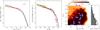 |
Fig. 1 Left panel: predicted luminosity function at z ≤ 0.1 (in bj band, solid line) compared with observations from Jones et al. (2006). Central panel: predicted local stellar mass function (solid line) compared with data from Baldry et al. (2012, squares), Li & White (2009, triangles), Panter et al. (2007, circles), and Fontana et al. (2006, diamonds). Right panel: the contour plot shows the predicted relative fraction of bulge-to-total mass as a function of the galaxy stellar mass. This is compared with data from Fisher & Drory (2011). The corresponding distribution of B/T ratios (differential number of objects per B/T bin, normalized to the total number, solid line) is also compared with the SDSS data (Lackner & Gunn 2012, shaded histogram) in the rightmost panel, for galaxies in the magnitude range −24 ≤ Mr ≤ −17. |
The above model constitutes our baseline for connecting the growth of BHs to the properties of their host galaxies. Thus, we first tested the updated version of our model to ensure it provides a reasonable account of the galactic properties and of their evolution over a wide range of cosmic times, assuming a concordance cosmology (see Spergel et al. 2007). In Fig. 1 we show how the model predictions compare with different local observables: the stellar mass function, the B-band luminosity function, and the ratio of the bulge to the total stellar mass. The good matching indicates that the model provides a fair description of both the (roughly) instantaneous and integrated star formation rates and that our treatment of stellar mass stripping and morphological transformations is consistent with observations.
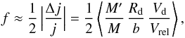
As a further test we show in Fig. 2 (left panel) the predicted local colour-magnitude distribution, which seems to capture the well known bimodal nature of the observed distribution. To quantify such a result, we compared in detail the predicted colour distribution of galaxies with different magnitudes (the right panel) with the SDSS (Sloan Digital Sky Survey) data. Besides the mentioned colour bimodality, the fraction of red galaxies continuously increases with increasing galaxy magnitude, as indicated by the data.
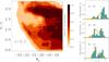 |
Fig. 2 Left panel: predicted local colour–magnitude relation. The colour code represents the number density of galaxies, normalized to the maximum value. Right panels: predicted colour distribution (differential number of objects per colour bin, normalized to the total number) for galaxies of different magnitudes (histograms) is compared with the data from the SDSS (Baldry et al. 2004, dots). |
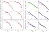 |
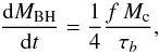
Fig. 3 Left panels: evolution of the K-band luminosity function predicted by the model (solid line) compared with the data from Cirasuolo et al. (2010, squares). Right panels: predicted evolution of the UV luminosity function (shaded region) compared with observed distribution of dropout galaxies. The shaded region encompasses the uncertainties due to the adopted extinction curve (Small Magellanic Cloud, Milky Way or Calzetti) In each redshift bin, the model galaxies have been selected according to the same selection criterium as adopted in the observations (see text). Data are taken from Reddy & Steidel (2009, dots), Bouwens et al. (2007, 2011, squares), and van der Burg et al. (2010, triangles). |
Finally, we tested that the evolution of the distribution of the K-band luminosity (a proxy for the stellar mass content) and of the UV luminosity (a proxy for the instantaneous star formation rate) are in reasonable agreement with the observations over the whole range of cosmic times where observations are available. This is done in detail in Fig. 3, where (in the left panel) we compare our results with the observed evolution of the K-band luminosity function from Cirasuolo et al. (2010) up to redshifts ≈3, and (in the right panel ) with the observed evolution of the UV luminosity functions of “dropout” galaxies from different authors (see caption) up to redshifts z ≈ 8. Since the latter depends strongly on the colour selection adopted to select the galaxy sample, we performed the same cuts in the colour–colour plane as adopted in the observations to select U-dropout galaxies at z ≈ 3 (Giavalisco et al. 2004) B-, V-, and I-dropouts (at z ≈ 4, z ≈ 5, z ≈ 6, respectively, see Bouwens et al. 2007), and infra-red dropouts at z ≥ 7 (Bouwens et al. 2011). To account for uncertainties related to adopted dust-extinction curve, our predictions are shown as shaded regions (see caption).
The comparisons above show that our semi-analytic model provides a reasonable statistical description of basic physical quantities (such as star formation rates, assembled stellar mass) that determine the cosmological evolution of the galaxy populations over a wide interval of cosmic times, so that it constitutes a solid “backbone” to connect the BH accretion (hence the ensuing AGN evolution) to the physical properties of their host galaxies, as we describe next.
3. Implementing the AGN feeding processes
We have updated our semi-analytic model to include two different modes for the BH accretion: i) an interaction-triggered (IT) mode, where the triggering of the AGN activity is external and provided by galaxy interactions (including both mergers and fly-by), which can provide – for major interactions – a large relative variation Δj/j of the angular momentum of the galactic gas; ii) a mode where accretion occurs due to disk instabilities, where the trigger is internal and provided by the break of the axial symmetry in the distribution of the galactic cold gas. In both cases, a nuclear star formation is associated to the accretion flow triggering the AGN.
Our modelling for the IT mode has been described in previous papers (starting from Menci et al. 2004, 2008; see also Lamastra et al. 2013b), so we only give a brief account of it, to recall its main properties. In this paper we expand on our implementation of the DI mode, which constitutes a novel component of the semi-analytic model. It is based on the HQ11 analytical model. Its detailed testing against high-resolution hydrodynamical N-body simulations (see HQ11; Anglés-Alcázar et al. 2013) makes it a reliable baseline for describing the accretion flow onto the BH within the limits of the present modelling of instabilities. We recompute the HQ11 model and extend it beyond the assumption originally adopted by HQ11 to assess its robustness and to compute the maximal impact that the DI mode can have on the evolution of the AGN population under different hypotheses.
3.1. The interaction-driven model
As implemented in other semi-analytic models, galactic clumps within a host halo undergo different processes. First, they lose angular momentum from the dynamical friction and eventually merge with the central galaxy; such a process is implemented in our model by adopting the standard Chandrasekar expression for the dynamical friction timescale given in Lacey & Cole (1993) that is adopted in most semi-analytic models (see also Somerville & Primack 1999; Cole et al. 2000; for variants of such a description see Somerville et al. 2012 and references therein).
In addition, satellite galaxies with any given circular velocity vc (and tidal
radius rt) may interact inside a host halo with
circular velocity V at a rate (Menci et al. 2002) 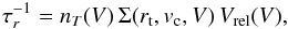 (1)where
nT is the number
density of galaxies in the host halo, Vrel the relative velocity between
galaxies, and Σ the cross
section for such encounters. The above expression yields the probability for fly-by
encounters (not leading to a merging) for a geometrical cross section
(1)where
nT is the number
density of galaxies in the host halo, Vrel the relative velocity between
galaxies, and Σ the cross
section for such encounters. The above expression yields the probability for fly-by
encounters (not leading to a merging) for a geometrical cross section
 , while it determines the
probability of a merging (binary aggregation) when the geometrical cross section is
suppressed by a factor ~
, while it determines the
probability of a merging (binary aggregation) when the geometrical cross section is
suppressed by a factor ~ , which
accounts for the requirement that the orbital energy is transferred into internal degrees
of freedom. The above appropriate cross sections are given by Saslaw (1985) in terms of the tidal radius rt associated to
a galaxy with given circular velocity vc (Menci et al. 2004). The binary merging of satellite galaxies is also implemented in
other semi-analytic models (see, e.g., Somerville & Primack 1999), and the tidal stripping of satellite galaxies is also included
in our model as described in Menci et al. (2012).
, which
accounts for the requirement that the orbital energy is transferred into internal degrees
of freedom. The above appropriate cross sections are given by Saslaw (1985) in terms of the tidal radius rt associated to
a galaxy with given circular velocity vc (Menci et al. 2004). The binary merging of satellite galaxies is also implemented in
other semi-analytic models (see, e.g., Somerville & Primack 1999), and the tidal stripping of satellite galaxies is also included
in our model as described in Menci et al. (2012).
The fraction f of cold gas destabilized by any kind of merging or
interaction has been worked out by Cavaliere & Vittorini (2000) in terms of the variation Δj of the specific angular
momentum j ≈
GM/Vd
of the gas to read (Menci et al. 2004) as
 (2)where
b is the
impact parameter, evaluated as the greater of the radius Rd and the
average distance of the galaxies in the halo, M′ is the mass of the partner galaxy in
the interaction, and the average is performed over the probability of finding such a
galaxy in the same halo where the galaxy with mass M is located. The
pre-factor accounts for the probability 1/2 of inflow rather than outflow related to the
sign of Δj.
The AGN and starburst events are triggered by all galaxy interactions including major
mergers (M ≃
M′), minor mergers (M ≪
M′), and fly-by events. We assume that in
each interaction, one fourth of the destabilized fraction f feeds the central BH,
while the remaining fraction feeds the circumnuclear starbursts (Sanders & Mirabel
1996). Thus, the BH accretion rate is given by
(2)where
b is the
impact parameter, evaluated as the greater of the radius Rd and the
average distance of the galaxies in the halo, M′ is the mass of the partner galaxy in
the interaction, and the average is performed over the probability of finding such a
galaxy in the same halo where the galaxy with mass M is located. The
pre-factor accounts for the probability 1/2 of inflow rather than outflow related to the
sign of Δj.
The AGN and starburst events are triggered by all galaxy interactions including major
mergers (M ≃
M′), minor mergers (M ≪
M′), and fly-by events. We assume that in
each interaction, one fourth of the destabilized fraction f feeds the central BH,
while the remaining fraction feeds the circumnuclear starbursts (Sanders & Mirabel
1996). Thus, the BH accretion rate is given by
 (3)where the
time-scale τb =
Rd/Vd
is assumed to be the crossing time of the destabilized galactic disk. The fraction of
destabilized gas in Eq. (2) is proportional
to the mass ratio M′/M
of the merging partners; thus for grazing, low speed encounters (Rd ≈
b and Vrel ≈ Vd)
major mergers (with M′/M ≈
1) may lead to a large relative variation in the gas angular momentum
Δj ≈
j and to a high accreted fraction f ~ 0.5.
(3)where the
time-scale τb =
Rd/Vd
is assumed to be the crossing time of the destabilized galactic disk. The fraction of
destabilized gas in Eq. (2) is proportional
to the mass ratio M′/M
of the merging partners; thus for grazing, low speed encounters (Rd ≈
b and Vrel ≈ Vd)
major mergers (with M′/M ≈
1) may lead to a large relative variation in the gas angular momentum
Δj ≈
j and to a high accreted fraction f ~ 0.5.
3.2. The disk instability model
In this section, we a) recall the key points in the HQ11 computation of the inflow rate onto the BH, performed for a power-law gas density profile; b) extend such a computation to treat different (exponential) gas density profiles; c) based on the HQ11 scenario we work out the star formation rate associated to a given BH accretion rate; and d) discuss how the computed accretion and star formation rates from disk instabilities actually represent upper limits to the real rates. In fact, in this work we are interested in investigating the maximal contribution that – according to present modelling – DI can give to the cosmological evolution of AGN, in order to constrain the evolution physical conditions where they may compete with, or even dominate, the contribution from galaxy interactions.
3.2.1. Computing the black hole accretion rate
As recalled in the Introduction, gas rich mergers and tidal interactions are not the only ways to produce a net mass inflow into the central region of the galaxies. In certain cases, secular growth processes such as disk instabilities (DI) might play a crucial role in feeding the central SMBH.
From a modelling point of view, describing such an accretion mode requires i) modelling
the DI trigger; and ii) modelling the corresponding inflow rate onto the BH. As for the
first, a widely used criterion for the onset of disk instabilities is that proposed by
Efstathiou et al. (1982) based on N-body simulations, which
states that a disk becomes unstable if its mass exceeds a critical value:
 (4)where
Rd the scale length of the disk, and
vmax is the maximum circular velocity
considering all the galaxy components. The latter is derived from velocity profiles
computed assuming a Navarro Frenk & White (1997, NFW) dark matter density profile, and it includes the effect of baryons
following Mo et al. (1998), as described in
Menci et al. (2005). Here ϵ
~ 0.5−0.75 is a parameter calibrated on simulations. The above
criterion is the one usually adopted in semi-analytic models: Hirschmann et al. (2012) adopt a value ϵ = 0.75, and a similar
value is adopted by Fanidakis et al. (2011). ITo investigate the maximum effect of DI on
the statistical evolution of AGN we also adopt the value ϵ = 0.75.
(4)where
Rd the scale length of the disk, and
vmax is the maximum circular velocity
considering all the galaxy components. The latter is derived from velocity profiles
computed assuming a Navarro Frenk & White (1997, NFW) dark matter density profile, and it includes the effect of baryons
following Mo et al. (1998), as described in
Menci et al. (2005). Here ϵ
~ 0.5−0.75 is a parameter calibrated on simulations. The above
criterion is the one usually adopted in semi-analytic models: Hirschmann et al. (2012) adopt a value ϵ = 0.75, and a similar
value is adopted by Fanidakis et al. (2011). ITo investigate the maximum effect of DI on
the statistical evolution of AGN we also adopt the value ϵ = 0.75.
Computing the mass inflow rate onto the BH, and the associated nuclear star bursts, is a more complex situation. At present, semi-analytical models only resort to ansatz tuned to maximize the model agreement with observations; in Hirschmann et al. (2012) the mass accretion rate is then calculated considering all the mass exceeding the threshold to be added in the central bulge and a tiny fraction of it (~10-3, motivated by the local BH-bulge mass relation) to be accreted in the central BH according to an exponential growth characterized by the Salpeter timescale. In the GALFORM model, Bower et al. (2006) and Fanidakis et al. (2012) assume that all the mass of the disk (not only the mass in excess) is added to the central bulge, leading to an enhanced effectiveness of the whole process. The lack of an analytical description of the complex physics processes acting in the transport of gas in the nuclear region means that the results strongly depend on the assumed prescriptions and may actually overestimate the actual inflows attainable in the central regions under realistic conditions.
Here we attempt to adopt a more physical treatment of the mass inflow from disk instabilities. In particular, we take on the analytical model proposed by HQ11, which aims at accounting for the physics of angular momentum transport and gas inflow from galactic scales (≈1 kpc) inwards where the BH potential is dominant. It considers the multi-component nature of the disk, and the inflow towards the BH is related to the nuclear star formation. In addition, such a model was tested by the authors against aimed hydrodynamical simulations, so that at present it constitutes a solid base for describing the BH accretion due to disk instabilities.
The model investigates the response of the disk to an external non-axisymmetric
perturbation of the potential Φa = | a |
Φ0, where the perturbation amplitude is | a | <
1. The unperturbed system corresponds to an axisymmetric thin disk
with a spherical component (BH, bulge and dark matter halo). While for periodic particle
orbits the net angular momentum loss vanishes at the first order in a, HQ11 show that the
shocks generated by gas particle in the condition of orbit crossing lead to a
first-order effect. As a result, in the orbit crossing (non-linear) regime, they obtain
the orbit-averaged gas inflow rate 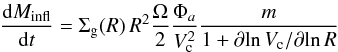 (5)where
Σg(R) is the gas surface density
profile; Ω the angular
velocity of the unperturbed disk, induced by both the bulge and the disk mass enclosed
within the radius R; Vc is the corresponding circular
velocity; m
is the mode of the perturbations (the perturbed potential is m-fold symmetric, so that
m = 0
corresponds to axial symmetry); and marginal orbit crossing is assumed following HQ11.
Here, our strategy is to maximize the effects of DI to single out the
wider range of physical conditions where such a process may be effective in fueling
AGNs. We therefore assume that when disk instabilities are triggered Eq. (5) always holds.
(5)where
Σg(R) is the gas surface density
profile; Ω the angular
velocity of the unperturbed disk, induced by both the bulge and the disk mass enclosed
within the radius R; Vc is the corresponding circular
velocity; m
is the mode of the perturbations (the perturbed potential is m-fold symmetric, so that
m = 0
corresponds to axial symmetry); and marginal orbit crossing is assumed following HQ11.
Here, our strategy is to maximize the effects of DI to single out the
wider range of physical conditions where such a process may be effective in fueling
AGNs. We therefore assume that when disk instabilities are triggered Eq. (5) always holds.
The mass inflow rate in Eq. (5) is of
first order in perturbation amplitude, since it depends linearly on Φa. To
calculate the exact value of the mass inflow rate, we need the analytic expression for
Φa and Σg. The former is obtained in
the WKB approximation where the disk dominates the potential, while it is related to the
BH mass in the inner region where the BH gravity is dominant (see Appendix A). The
latter can be estimated assuming an equilibrium between mass inflow rate due to the disk
instability and star formation rate (described in terms of its surface density
Σ∗):
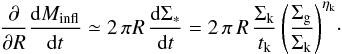 (6)The
last equality follows after relating the star formation surface density Σ∗ to the gas surface density
Σg through the
Schmidt-Kennicut law dΣ∗/ dt =
(Σk/tk) ∗
(Σg/
Σk)ηk, where the
timescale tk, the normalization Σk and the exponent
ηk are derived from fits to the
observations: typical values (Bouché et al. 2007)
are tk ≈ 0.4 ×
109 yr, Σk ≈ 108 M⊙ kpc-2, and ηk = 1.7, but
the real slope ηk is still subject to different
observational estimates in the range 1.2 ≲
ηk ≲ 1.8 (see, e.g., Davies et al.
2007; Hicks et al. 2009; Daddi et al. 2010;
Genzel et al. 2010; Santini et al. 2014), also depending on the redshift and on the
properties of the adopted galaxy sample.
(6)The
last equality follows after relating the star formation surface density Σ∗ to the gas surface density
Σg through the
Schmidt-Kennicut law dΣ∗/ dt =
(Σk/tk) ∗
(Σg/
Σk)ηk, where the
timescale tk, the normalization Σk and the exponent
ηk are derived from fits to the
observations: typical values (Bouché et al. 2007)
are tk ≈ 0.4 ×
109 yr, Σk ≈ 108 M⊙ kpc-2, and ηk = 1.7, but
the real slope ηk is still subject to different
observational estimates in the range 1.2 ≲
ηk ≲ 1.8 (see, e.g., Davies et al.
2007; Hicks et al. 2009; Daddi et al. 2010;
Genzel et al. 2010; Santini et al. 2014), also depending on the redshift and on the
properties of the adopted galaxy sample.
There could be situations where the equilibrium described by Eq. (6) does not hold: when star formation inhibits the mass inflow completely, or when the gas inflow rate is higher than star formation (Barnes & Hernquist, 1991). However, we later show that these two different regimes yield a mass inflow onto the central BH weaker than inflow obtained when the equilibrium is reached. Since our aim is to study the maximum effects of DI on the cosmological evolution of AGN, we retain the above approach.
With Eqs. (5) and (6) it is possible to solve for both the gas
density (hence for the star formation) and the mass inflow. To this aim (see Appendix A
for a step-by-step computation), the potential (hence Φa in Eq.
(5)) has to be evaluated in two
regions: an outer region where the disk gravity is dominant, and an inner region where
gravitational potential is dominated by the BH. The radius RBH ~
10−100 pc (depending on
the BH mass) marks the separations between the two regions, while the scale
Racc ~
10-2−10-1 pc corresponds to the inner bound
of the innermost regions; inside this radius, star formation ceases and the mass inflow
can be assumed to be almost constant. The mass inflow at this radius Ṁinfl(Racc)
corresponds to the final BH accretion rate that we include in our semi-analytic model.
The computation of such a quantity is given in detail in Appendix A, where it is
expressed in terms of quantities evaluated far from the very central region, at a
“galactic” scale R0 ~ 100−1000 pc, so that the
central BH accretion rate can be easily connected to the galactic properties of the host
galaxy computed in our semi-analytic model. This is done in Appendix A for a power-law
scaling of the disk surface density Σd ~ R−
ηd and in Appendix B for an
exponential disk profile. In the first case, ηd is calibrated on N-body simulations: our
fiducial choice is to take the best-fitting value ηd = 1 /
2 given by HQ11. Then, for a Kennicut-Schmidt index ηk = 7 /
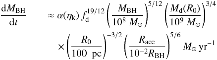
4 (as adopted by HQ11) the final result is ![Mathematical equation: \begin{align} \label{hopkins} &\frac{{\rm d}M_ {\rm BH}}{{\rm d}t} \equiv \frac{{\rm d}M_ {\rm infl} (R_{\rm acc})}{{\rm d}t} \approx {\alpha(\eta_{\rm k},\eta_{\rm d}) \, f_{\rm d}^{4/3}\over 1+2.5\,f_{\rm d}^{-4/3}(1 + f_0/f_{\rm gas}) } \left( \frac{M_{\rm BH}}{10^8~M_{\odot}}\right)^{1/6}\nonumber\\ &\quad\quad \quad\quad\times \left( \frac{M_{\rm d}(R_0)}{10^9~M_{\odot}}\right) \left( \frac{R_0}{100~{\rm pc} }\right) ^{-3/2} \left( \frac{R_{\rm acc}}{10^{-2}R_{\rm BH}}\right) ^{5/6} M_{\odot}\,{\rm yr}^{-1} \\ &f_0 \approx 0.2 f_{\rm d}^2 \left[ \frac{M_{\rm d}(R_0)}{10^9~M_{\odot}}\right]^{-1/3} {\hspace{1cm}} f_{\rm gas} \equiv {M_{\rm gas} (R_0)\over M_{\rm d}(R_0)}\cdot \end{align}](/articles/aa/full_html/2014/09/aa24217-14/aa24217-14-eq114.png) Here
MBH is the central BH mass,
fd is the total disk mass fraction, and
Md and Mgas are the
disk and the gas mass calculated in R0. For physical values of
0 ≤ fd ≲
0.5, the above equation yields accretion rates that are
indistinguishable from the original formulation given in HQ11. The above equation
relates the BH accretion at the sub-resolution scale Racc to
quantities evaluated at the galactic scale R0 which are computed for each galaxy
by the semi-analytic model described in Sect. 2. Under the assumptions adopted by HQ11 –
the product
Here
MBH is the central BH mass,
fd is the total disk mass fraction, and
Md and Mgas are the
disk and the gas mass calculated in R0. For physical values of
0 ≤ fd ≲
0.5, the above equation yields accretion rates that are
indistinguishable from the original formulation given in HQ11. The above equation
relates the BH accretion at the sub-resolution scale Racc to
quantities evaluated at the galactic scale R0 which are computed for each galaxy
by the semi-analytic model described in Sect. 2. Under the assumptions adopted by HQ11 –
the product  is
constant (as shown in our Appendix A), so that Eq. (6) can be evaluated at any radius R0, provided
it remains within the range where the adopted assumptions for the scaling of the stellar
disk surface density remain valid (R0 ≲ 1 kpc). The constant
α(ηk,ηd)
~ 0.1−5 is given in Eq. (A.14) and parameterizes the strong dependence of the normalization on the
exact value of ηk of the Schmidt-Kennicutt law (see
Appendix A). To maximize the contribution of the DI mode to the
evolution of AGN, in the following we shall keep such a parameter to a maximum value
α(ηk,ηd)
= 10. Finally, following HQ11, we assume Racc to be
equal to ~10-2RBH.
is
constant (as shown in our Appendix A), so that Eq. (6) can be evaluated at any radius R0, provided
it remains within the range where the adopted assumptions for the scaling of the stellar
disk surface density remain valid (R0 ≲ 1 kpc). The constant
α(ηk,ηd)
~ 0.1−5 is given in Eq. (A.14) and parameterizes the strong dependence of the normalization on the
exact value of ηk of the Schmidt-Kennicutt law (see
Appendix A). To maximize the contribution of the DI mode to the
evolution of AGN, in the following we shall keep such a parameter to a maximum value
α(ηk,ηd)
= 10. Finally, following HQ11, we assume Racc to be
equal to ~10-2RBH.
Since our semi-analytical model uses exponential-law density profiles to describe the
disk surface density profile (at galactic scales), we have also developed all the
calculations for the case of “exponential disks”. The resulting mass inflow rate is
 (9)with
Rd the exponential length of the disk,
and all the calculations for exponential disks are shown in Appendix B. All the factors
in Eq. (9) are the same of Eq. (6); α(ηk,ηd)
= 0.1−1.2 (depending on ηk) is now given by Eq. (A.14) with ηd = 0. With
the choice Racc ~
10-2RBH, the inflow is quite
insensitive to the exact values of Racc and RBH; however,
when it is necessary (see next section), we eventually take Racc ~ 0.1 pc
and RBH ~
10 pc.
(9)with
Rd the exponential length of the disk,
and all the calculations for exponential disks are shown in Appendix B. All the factors
in Eq. (9) are the same of Eq. (6); α(ηk,ηd)
= 0.1−1.2 (depending on ηk) is now given by Eq. (A.14) with ηd = 0. With
the choice Racc ~
10-2RBH, the inflow is quite
insensitive to the exact values of Racc and RBH; however,
when it is necessary (see next section), we eventually take Racc ~ 0.1 pc
and RBH ~
10 pc.
3.2.2. Computing the nuclear star formation rate
Since the above models assume equilibrium between mass inflow and star formation, a star formation activity is always connected to the BH acccretion rate given in Eqs. (6) or (9), and can be computed in detail after Eq. (6), as shown in Appendix A. As a result, a star formation rate Ṁ∗ ,DI = A∗ ,DIṀBH is obtained, where the exact value of the proportionality constant A∗ ,DI ≳ 102 depends on the detailed radial profile of the disk potential and of the gas surface density. The effects of changing A∗ ,DI within the limits derived in Appendices A and B will be quantitatively shown in the next section. Here we note that, given a total amount of baryons available for accretion, increasing A∗ ,DI leads to a faster gas consumption, and hence to a lower accretion rates at subsequent times, with the effect of decreasing the number of active AGNs. Thus, to investigate the maximum impact of the DI mode on the growth of BHs and on the evolution of AGNs it is sufficient to adopt proper lower limits for the DI star formation rate. This can be done within the framework of the DI model introduced above, and the derivation is shown (Appendix A, B) for both a power law and an exponential profile of the disk surface density. We obtain a lower limit A∗ ,DI = 100 (Eq. (A.18)) for a power-law profile (see Sect. A.5), corresponding to the contribution to the star formation from the inner region R ≲ RBH. This also constitutes a lower limit for the case of an exponential disk, since in the inner region, the potential determining the mass inflow is dominated by the BH and does not depend on the assumed disk profile (see also Appendix B, Eqs. (B.11)−(B.13)). The contribution to the star formation rate from outer regions depends strongly on the assumed disk surface density; in the case of a power-law profile, larger and larger contributions are obtained when the power-law behaviour is extrapolated to regions far from the nucleus (see Eqs. (A.19)−(A.22)), while in the case of an exponential profile (more realistic in regions far from the BH sphere of influence R ≫ RBH) we obtain an additional contribution saturating to A∗ ,DI = 60.
4. Results
We compute separately the effects of the two accretion modes on the AGN population. To
compare with observations, the AGN bolometric luminosity is computed as 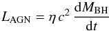 (10)where
dMBH/ dt
is taken from Eq. (3) for the IT mode, and
from Eq. (6) (or Eq. (9)) for the DI models. We adopt an
energy-conversion efficiency η =
0.1 (see Yu & Tremaine 2002). The luminosities in the UV and in the X-ray bands are computed from the
above expression using the bolometric correction given in Marconi et al. (2004).
(10)where
dMBH/ dt
is taken from Eq. (3) for the IT mode, and
from Eq. (6) (or Eq. (9)) for the DI models. We adopt an
energy-conversion efficiency η =
0.1 (see Yu & Tremaine 2002). The luminosities in the UV and in the X-ray bands are computed from the
above expression using the bolometric correction given in Marconi et al. (2004).
We stress again that in the present work we do not attempt to find a best-fitting combination of the two accretion modes. Rather, we are interested in isolating the effects of the two accretion modes on the evolution of the AGN population, to single out the physical regimes where they may be effective in driving the AGN evolution. Given that in our previous paper (and in the following results), the IT mode has been shown to be able to provide acceptable fits to the observed evolution of the AGN population, our strategy will be to maximize the possible DI accretion rates in order to assess whether and for what kind of object we expect it to be competitive with the IT mode. To this aim, we explore the possible variants of the DI model provided by different choices for i) the normalization α(ηK,ηd) in Eq. (6), which in turn is related to the present uncertainties concerning the slope of the Kennicut-Schimdt law ηk; ii) the different disk surface density profiles, determining the slope ηd (see Sect. 3.2.1) and the dependence of ṀBH on both the disk mass fraction and the gas fraction (through the boundary condition A(RBH) in Appendix A; iii) the star formation associated to the DI mode and discussed in Sect. 3.2.2.
These quantities are not freely tunable, since they can only vary within limits set by observations and simulations. The former set a limit for the Kennicut-Schmidt index 3 / 2 ≤ ηk ≤ 7 / 4 (see Sect. 3.2.1). The latter provide a range of possible gas surface density profiles ranging from Σg ~ R-3 to Σg ~ R-1, bracketing the effects of the present uncertainties in the physics of the inter-stellar medium (see Hopkins & Quataert 2010). These mainly concern the effective equation of state of the gas, which widely varies from cases where it is quite stiff on small scales (near-adiabatic, similar to what is adopted in the studies of Mayer et al. 2007; Dotti et al. 2009), through cases where the gas is allowed to cool to a cold isothermal floor and forms a clumpy, inhomogeneous medium (on galactic scales, similar to what is assumed in Bournaud et al. 2007; Teyssier et al. 2010), and includes cases where the gas motions gain a significant contribution from resolved turbulent motions, and the gas mass distribution can be highly inhomogeneous and clumpy. The above range of uncertainty for the gas surface density profiles translates (Eqs. (A.1), (A.2), (B.8)) into values ranging from ηd = 1 / 2 (the HQ11 case) to ηd = 0 (our exponential case).
For the above ranges of uncertainty 3 / 2 ≤ ηk ≤ 7 / 4 and 0 ≤ ηd ≤ 1 / 2, the normalization of the BH accretion rates in Eqs. (8) and (9) remains in the range 0.1 ≲ α(ηk,ηd) ≤ 5 (see Sect. 3.2.1). To investigate the maximum impact of DI, we adopt a safe normalization α(ηk,ηd) = 10, the same as is considered by HQ11 to constitute a definite upper limit. A final source of uncertainty comes from the contribution to the nuclear star formation rate from regions outside the BH sphere of influence R ≥ RBH. Assuming it to be zero sets a lower limit A∗ ,DI = 100 for the normalization of the nuclear star formation rate, which maximizes the amount of inflowing gas feeding the BH accretion, as discussed in Sect. 3.2.2. We refer to the combination α = 10 and A∗ ,DI = 100 as “maximal” DI model. In addition, we also explore the effect of the additional contribution to the nuclear starbursts from regions far from the BH sphere of influence.
In sum, following the lines above, we explore three variants of the DI mode:
-
a fiducial case corresponding to the model adopted by HQ11(Eq. (6)), computed assuming a power-law disksurface density profile ηd = 1 / 2 with a maximized value of the parameter α(ηK,ηd) = 10 (see Sect. 3.2.1), and assuming the lower limit for the associated star formation rate A∗ ,DI = 100 (see Sect. 3.2.2 and Appendix A).
-
the case of an exponential profile for the disk surface density (Eq. (9)), keeping the same values for α(ηK,ηd) = 10 and A∗ ,DI = 100 (see Sect. 3.2.2 and Appendix B).
-
a model with enhanced star formation rate associated to DI (for a power-law profile). It assumes a normalization of the star formation associated to DI above the lower limits derived in Sect. 3.2.2, with an additional contribution A∗ ,DI = 100 from regions far from the BH sphere of influence (R ≫ RBH).
Having defined our reference set of DI cases, we proceed to study the evolution of the AGN population under different triggering models.
4.1. Evolution of the AGN luminosity function and BH mass function
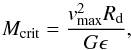
The evolution of the AGN UV luminosity funtions predicted in the IT scenario is compared with the one corresponding to the DI mode in Fig. 4. The luminosity functions are computed in the UV band at λ = 1450 Å, where most of the UV rest frame data on AGN are collected and where the average AGN emission shows the peak in the spectral energy distribution, which is representative of the overall bolometric emission. The predictions are compared with data taken from different bands, including the X-ray data (corrected for obscuration) by La Franca et al. (2005); Ebrero et al. (2009) at low redshifts z ≲ 1.5, the X-ray data for objects in the COSMOS field by Brusa et al. (2010); Civano et al. (2011); and the Chandra X-ray data for objects detected at z ≥ 4 in the GOODS south field by Fiore et al. (2012). These are converted to the UV with the bolometric corrections in Marconi et al. (2004). Details on the conversion procedure are given in Fiore et al. (2012) and Giallongo et al. (2012).
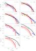 |
Fig. 4 Predicted evolution of the AGN luminosity function in the UV band (at 1450 Å). Solid black lines refer to the IT scenario, and red solid lines to the DI model. We also plot variants of the DI model: dashed lines refer to the DI model computed with an exponential profile, while dotted lines to the DI model with increased star formation (see text). We compare with observed UV luminosity functions by Richards et al. (2006, solid squares), Croom et al. (2009, solid circles at z< 3 ), Siana et al. (2008, open squares), Bongiorno et al. (2007, open circles), Fontanot et al. (2007, solid diamonds), Glikman et al. (2011, big filled circles at z = 4.25), Jiang et al. (2009; solid squares at z ≥ 6). We also include luminosity functions from X-ray observations, converted to UV through the bolometric corrections in Marconi et al. (2004): the shaded region brackets the determinations derived in the X-ray band at z ≤ 2 by La Franca et al. (2005), Ebrero et al. (2009), Aird et al. (2010), while at higher redshifts we plot data from Fiore et al. (2012, penthagons), Brusa et al. (2010, triangle), Civano et al. (2011, green empty squares). |
The results shown in Fig. 4 indicate that none of the variants of the DI mode can provide the accretion needed to obtain high-luminosity QSO with M1450 ≤ −26, especially at redshifts z ≳ 3.5. This is because the accretion rates in Eqs. (6) and (9) have a mild dependence on the BH mass, but depend very strongly on the disk mass fraction and on the gas mass fractions (fd and fgas). Thus, in galaxies with a relatively low gas fraction, or in galaxies with a large B/T ratio, the DI mode is more suppressed than the IT mode. As expected DI can instead be very effective in the range of galaxy masses (and AGN luminosities) dominated by disk galaxies −25 ≲ M1450 ≲ −22. While we must keep in mind that the predicted DI luminosity functions in Fig. 4 constitute upper limits, the results show that in such a magnitude range the DI accretion rates could compete with – or even overtake – those attained in the IT scenario, at least for redshifts z ≲ 3.5. At higher redshifts, although galaxies are surely gas rich with large fgas ~ 1, the typical disk mass fraction fd decreases since – in the standard scenario assumed in semi-analytic models – the frequent major interactions continuously disrupt the forming disks.
Within the assumed modelling for the inflow driven by DI, our fiducial DI case constitutes an effective upper limit for the bright end of the luminosity function. Increasing the associated star formation A∗ ,DI above the lower limit A∗ ,DI = 100 would yield lower luminosity functions, as shown in Fig. 4, for the reasons explained in Sect. 3.2.2. Changing the disk power-law density profile assumed in the original version of HQ11 to an exponential profile also results in a lower abundance of bright AGN. Indeed, the same fiducial model must be regarded as an effective upper limit, since the assumed value for the normalization α(ηK,ηd) = 10 is actually appreciably higher than any value attained with realistic values of ηk and ηd, as shown in Appendix A (see Eq. (A.14) and the text below).
For the IT model, the results presented here are very similar to those obtained in the earlier version of our model (see, e.g., Giallongo et al. 2012), and show an acceptable matching with the data. For z ≥ 4.5 the real size of the model over-prediction with respect to the faintest data points still has to be assessed. In fact, the observations by Fiore et al. (2012) could be affected by several uncertainties and significant incompleteness. The objects have been selected from very deep Hubble Space Telescope near infrared images at H ≈ 27 and measured at the faintest X-ray fluxes of FX ≈ 2 × 10¹⁷ erg s-1 cm-2. At the lowest X-ray luminosities, objects with relatively high X/optical ratio, and consequently with H > 27, are lacking in their survey. As a consequence, uncertainties in the Fiore et al. (2012) luminosity functions data due to systematic errors could be larger than shown in the figure based on number statistics.
While the above result strongly disfavour DIs as the dominant accretion mode in high-luminosity AGNs, they also indicate that it could be as effective as the IT mode (or even more) in intermediate-luminosity AGNs especially at intermediate redshifts 2 ≲ z ≲ 3.5. This is the epoch where massive star formation – possibly triggered by DI in gas-rich objects – is observed in disk galaxies (Bournaud et al. 2007; Genzel et al. 2008). Thus, we can seek proper observables able to assess whether one of the two modes clearly dominates in this luminosity and redshift range.
A possible approach could be to seek for signatures in the BH mass function and/or in the MBH − M∗ relation. The former statistically describes the growth of BH masses corresponding to the evolution of the BH accretion rates shown in Fig. 4. Our predictions for such a quantity are presented for both the IT and the fiducial DI models in Fig. 5. At low redshifts the predictions are compared with a compilation of data (Shankar et al. 2009). While current data do not allow to distinguishing between the DI and the IT scenario at low redshift z ≲ 0.3, the predicted evolution of the BH mass funtions differs appreciably at higher redshifts; in particular, as expected from the evolution of the AGN luminosity functions, DI provide a much lower abundance of massive BH at z ≳ 1.
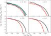 |
Fig. 5 Predicted evolution of the BH mass function in the IT scenario (solid black lines) and in the DI model (solid red line). The shaded region defines the spread in observational estimates obtained using different methods, as compiled by Shankar et al. (2009). |
4.2. The MBH − M∗ relation
A larger difference between the IT and the DI prediction is shown by the local MBH − M∗ relation, shown in Fig. 6. While both the IT and the DI accretion modes provide a local relation consistent with observations, the slope and – most of all – the scatter differ appreciably. While present data do not allow a clear preference for one of the two modes, it is interesting to note that the large scatter characteristic of the IT mode comes from the variance in the merging histories, which has a strong impact in a model where interactions provide the trigger and the power of the AGN emission; the origin of such a variance can be visualized through the paths followed by AGN host to reach their final position in the MBH − M∗ plane.
Such paths include situations in which the progenitor of present-day massive BH are characterized by an early accelerated phase of BH growth, which brings them above the local relation at early times z ≳ 4, followed by a later phase where the BH growth appreciably decelerates while the “quiescent” star formation gradually increases the stellar content of their host galaxies, and these paths are those leading to the early building up of large-mass BHs at high redshifts z ≳ 4. The paths passing below the local relation instead correspond to galaxies retaining a large fraction of their gas down to late cosmic epoch, so that they form stars at very high rates down to z ≈ 2 (the most star forming objects are those corresponding to SMG, see Lamastra et al. 2010). Such a large variance in the paths leading to the local relation is missing in the DI scenario, where the trigger and the accretion rate of AGN are provided by internal properties which are less prone to the merging history. Indeed, in the DI the paths are confined in a small region of the plane; the growth of BH follows a corresponding growth of the stellar mass content, and phases where either ṀBH or Ṁ∗ largely dominate are absent. This means that we expect a tight correlation between the AGN luminosity and the star formation rate in the host galaxy. This constitutes an interesting point that we shall investigate in detail in a following paper.
4.3. The distributions of the Eddington ratio
The different paths characterizing the BH growth in the IT and DI models suggest that the specific growth rate ṀBH/MBH could constitute an effective quantity for distinguishing the two modes; thus, we investigated how the distributions of Eddington ratio λ = LAGN/LEdd (here LEdd ∝ MBH is the Eddington luminosity, and LAGN ∝ ṀBH after Eq. (10)) compares with present observations. The result is presented in Fig. 7, where the AGN bolometric luminosity is shown as a function of the BH masses for the IT and DI scenarios, in two redshift bins. Luminosities corresponding to Eddington ratios λ = 1, λ = 10-1, and λ = 10-2 are also shown. Here the distributions appear substantially different when the IT or the DI modes are assumed. In the former case, a wide spread is present for most of the explored luminosity range, while the average value of λ increases with increasing LAGN, to reach values λ ≈ 1 at the highest luminosities. Conversely, for the DI scenarios the distributions are characterized by average values of λ increasing for decreasing luminosities and by a small scatter. This is expected, owing to the tighter region of the parameter space (gas rich fgas ~ 1, disk dominated fd ~ 1 dominated galaxies) where the DI mode is expected to be effective after Eq. (6), and also to the smaller variance associated to the merging histories when an internal trigger is assumed, as we discussed above. We compare our predictions with data from Rosario et al. (2013a,b), derived from spectroscopically observed AGN in the COSMOS field at 0.5 < z < 2.2 with reliably BH mass estimates from multiple optical spectroscopic surveys: the Sloan Digital Sky Survey (DR7; Abazajian et al. 2009), the zCOSMOS bright and deep surveys (Lilly et al. 2007), Magellan/IMACS program (Trump et al. 2009). BH masses were computed using virial relationships and Hβ and MgII emission lines (Trakhtenbrot & Netzer 2012), while bolometric luminosities were estimated using bolometric corrections to the monochromatic luminosities at either 5100 Å or 3000 Å rest frame. The choices of bolometric corrections are derived in Trakhtenbrot & Netzer (2012) and are consistent with the prescriptions of Marconi et al. (2004).
We note that at low AGN luminosities the comparison with data is affected by the observational bias set by the flux limit of the sample. This corresponds to LAGN ~ 1044.2 erg/s at z = 0.5−1 and LAGN ~ 1044.7 erg/s at z = 1.5−2. At low redshift z = 0.5−1, where the flux limit could still allow the low-luminosity end of the distribution to be probed, the comparison with the model is affected by the paucity of data points. This is due to a further selection bias, since the zCOSMOS AGN, which statistically dominate the sample, were specifically chosen to include the MgII line, which enters into the wavelength range of the zCOSMOS bright spectra at z ~ 1.
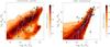 |
Fig. 6 Local MBH − M∗ relation for the IT model (left panels) and the DI model (right panels). Data points represent the observed local relation from Häring & Rix (2004, diamonds), and Marconi & Hunt (2003, squares, here M∗ is derived using the best-fitting virial relation of Cappellari et al. 2006); the colour code represents the fraction of AGN as a function of MBH for any given value of M∗, as indicated by the colour bar. We also show some of the paths in the MBH(t) − M∗(t) plane followed, during their evolution, by BHs (and by their host galaxies) reaching a final mass of MBH(z = 0) ≥ 109 M⊙. |
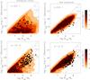 |
Fig. 7 Predicted distribution of AGN in the LAGN − MBH plane for the IT (left) and DI (right) models is compared with data from Rosario et al. (2013a,b) in two redshift bins. The lines corresponding to Eddington ratio λ = 1, λ = 0.1 and λ = 0.01 are also indicated. |
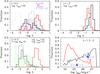 |
Fig. 8 Top left panel: predicted distributions of the Eddington ratio λ in the IT (solid black line) and DI (solid red line) scenarios for AGN with bolometric luminosity LAGN< 1046 erg s-1 at z ≤ 0.5. They are compared with different sets of data (see text for details): a sample of X-ray-selected AGN (dashed violet histogram), of IR-selected (dashed histogram) and Radio selected AGN (dotted histogram) from Hickox et al. (2009), and the sub-sample of X-ray and IR AGN from Kollmeier et al. (2006, dark green histogram) corresponding to z ≤ 0.5. Top right panel: as above, but for luminous AGN with LAGN> 1046 erg s-1 at z ≤ 1.2. The dashed histogram represents observational results from Kollmeier et al. (2006). Bottom left panel: as above, but for AGN with BH masses in the range 107 M⊙ ≤ MBH ≤ 08 M⊙. Here we compare with data from Kauffmann & Heckman (2009, histogram). Bottom right panel: fraction of AGN with high Eddington ratios λ ≥ 0.5 as a function of the AGN bolometric luminosity LAGN, at z = 2. As above, the solid black line corresponds to the IT mode and the solid red line to the DI case. The points are computed from the data by Rosario et al. (2013a,b) shown in Fig. 7. |
Since the distribution of AGN in the LAGN − MBH plane is appreciably different for the DI and IT cases, a possible way of determining which of the two modes dominates the accretion for intermediate- and low-luminosity AGN could consist in comparing the corresponding distributions of Eddington ratios λ with present observations at low redshifts, where low-luminosity objects are accessible to observations; in fact, for such AGN, the IT mode is expected to yield distributions with larger variance and skewed to values 10-2 ≲ λ ≲ 10-1, while higher values of λ and less scatter are expected for the DI mode.
However, when the model predictions for the two modes are compared with the data (see Fig. 8) we face with a complex situation; in fact, the observational distributions (at least) depend on i) the method adopted to select AGN; ii) the adopted bolometric correction; iii) the method adopted to measure the BH mass (for a discussion of the above points, see, e.g., Netzer et al. 2009a,b and references therein). This is illustrated in the top left-hand panel, where we compare with low-redshift data for AGN with LAGN < 1046 erg s-1 taken from Hickox et al. (2009) and Kollmeier et al. (2006). The former refer to AGN at 0.25 < z < 0.8 selected in different wavebands. The radio data are taken from the Westerbork Synthesis Radio Telescope 1.4 GHz radio survey (de Vries et al. 2002), the X-ray data are from the XBootes survey, covering the full AGES (AGN and Galaxy Evolution Survey) spectroscopic region (Murray et al. 2005; Kenter et al. 2005), while the mid-infared data are from the Spitzer IRAC Shallow Survey covering the full AGES field in all four IRAC bands (Eisenhardt et al. 2004). The authors base their estimate MBH on the LB,bul − MBH relation after estimating the bulge luminosity of the host galaxy in the B band, while the bolometric luminosity for X-ray AGN are derived from the bolometric correction of Hopkins et al. (2007); for radio AGNs that are not detected in X-rays, they used the X-ray stacking results to derive approximate upper limits on the X-ray AGN luminosity, while for IR AGNs that are not detected in X-rays, Lbol is derived from the rest-frame 4.5 μm luminosity. We also compare this with data from Kollmeier et al. (2006), derived from the AGES survey and consisting of X-ray (XBootes survey, Murray et al. 2005, Kenter et al. 2005) or mid-infrared (Eisenhardt et al. 2004) point sources with optical magnitude R ≤ 21.5 mag and optical emission-line spectra characteristic of AGNs. Black hole masses were estimated using virial relationships and Hβ MgII, and CIV emission-line widths, while bolometric luminosities were estimated using the bolometric correction of Kaspi et al. (2000) to the monochromatic luminosities at 5100 Å.
The comparison in Fig. 8 (top-left panel) shows that, while a marked difference is indeed apparent between model predictions for the IT mode and the DI mode, the observational distributions for X-ray-selected AGN (Hickox et al. 2009) extend to lower values of λ with respect to IR AGN, while radio-selected objects show a distribution peaked to much lower values of λ. While the X-ray homogeneous sample in Hickox et al. (2009) would favour the IT accretion mode, the mixed IR+X-ray data by Kollmeier et al. (2006) are instead best matched my the DI mode predictions, showing the impact of adopting different methods to measure BH masses on the comparison with model predictions. Again scatter constitutes a crucial diagnostics for pinning down the dominant accretion mode for low- and intermediate- luminosity AGN (see also Shankar et al. 2013). Much weaker constraints come instead from luminous AGN (top-left panel), where the two modes yield similar distributions and scatter. For luminous AGN, however, we know from the results in Fig. 4 that IT mode must dominate, since accretion from DI does not provide the observed abundance of bright AGN.
We also compare (Fig. 8, bottom left panel) with data for low-mass BHs (107 ≤ MBH/ M⊙ ≤ 108) taken from Kauffmann & Heckman (2009). Their sample is drawn from the Data Release 4 of the SDSS at z ≃0.2 (York et al. 2000; Adelman-McCarthy et al. 2006). AGN are identified from their position in the [O III](λ = 5007 Å)/Hβ versus [N II](λ = 6583 Å)/Hα diagram, as discussed in Kauffmann et al. (2003). Here LAGN is derived from the luminosity LOIII of the [OIII](λ = 5007Å) line after applying a bolometric correction that they estimate in the range 500−800, while BH masses were estimated using the stellar velocity dispersions measured from the SDSS spectra and the formula given in Tremaine et al. (2002). Within the limitations of available data − affected by substantial uncertainties concerning the bolometric correction, the measurements of the BH mass, and selection effects − the spread and the peak of the observed distribution seem to favour the IT scenario, but conclusive evidence is still missing. Also λ-distributions with a large spread are indicated by analysis of the observed AGN duty cycles (see Shankar et al. 2013).
Thus, at present the observational situation does not allow defining a definite distinction between the DI and the IT accretion modes. The key point is to assess whether low- and intermediate- luminosity AGN have a narrow distribution of λ peaked at λ ~ 1 (as predicted for the DI mode) or a wider distribution extending to λ ~ 10-1−10-2. Thus, a straightforward observational test is constituted by the fraction of AGN with high (λ ≥ 0.5) Eddington ratios as a function of the AGN luminosity (choosing a redshift bin where significant statistics is ensured, 2 ≤ z ≤ 3). The opposite behaviour is then predicted when IT and DI are assumed as dominant accretion modes, as shown in the bottom right-hand panel of Fig. 8. We stress again that, while the dominance of the IT mode for bright AGN results from the luminosity functions in Fig. 4, the interesting test is constituted by the low-luminosity region of the plot, where an increasing fraction for lower luminosities would clearly point towards the effectiveness of DI in triggering AGN; however, present data (taken by integrating the LAGN − MBH data by Rosario et al. 2013a,b shown in Fig. 7) – although consistent with a dominance of the IT mode for luminous AGN – still do not allow probing the low-luminosity range. Measuring such a quantity and comparing it with the predicted distributions could provide a clear observational test to assess whether DI may be the dominant accretion mode for intermediate-low AGN luminosities.
5. Discussion and conclusions
Using a a state-of-the-art semi analytic model for galaxy formation, we have made a detailed investigation of the effects of accretion triggered by disk instabilities (DI) in isolated galaxies on the evolution of the AGN population and on the corresponding growth of massive BHs. Specifically, we took on, developed, and expanded the Hopkins & Quataert (2011, HQ11) model for the mass inflow following disk perturbations, based on a physical description of nuclear inflows and tested against aimed N-body simulations.
We compared the evolution of AGNs due to this DI accretion mode with that arising in a scenario where galaxy interactions produce the sudden destabilization of large quantities of gas feeding the AGN (interaction-triggered – IT – mode). This constitutes the standard AGN feeding mode implemented in the earliest versions of our semi-analytic model, and has was extensively tested in our previous works. Here we did not attempt to develop a best-fitting model including both accretion modes, but rather we investigated the effects of assuming DI or IT as dominant modes studying the maximal contribution of DI to the evolution of the AGN population, within the framework of the HQ11 model for nuclear inflow. To this aim, we extended and developed the HQ11 model for DI to assess the effects of changing the assumed disk surface density profile and the associated nuclear star formation rates within the limits provided by N-body simulations. The goal was to investigate how often and to what extent the galaxy properties evolving in a cosmological context (and described through a semi-analytic model) provide the nuclear inflows associated to disk instabilities in ultra-high resolution simulations. We obtained the following results:
-
For luminosity M1450 ≳ −26 AGN, the DI mode can provide the BH accretion needed to match the observed AGN luminosity functions up to z ≈ 4.5. In such a luminosity range and redshift, it constitutes a viable candidate mechanism for fueling AGN, and can compete with the IT scenario as the main driver of the cosmological evolution of the AGN population.
-
The DI scenario cannot provide the observed abundance of high-luminosity QSO with M1450 ≤ −26 AGN, as well as the abundance of high-redshift z ≳ 4.5 QSO with M1450 ≤ − 24. This is because the strong dependence of the BH accretion rate on the gas fraction fgas and on the B/T ratio in the HQ11 model limits the effectiveness of such an accretion mode in massive galaxies; at high redshifts, the frequent major mergers predicted to take place at high redshifts z ≳ 5 in the host galaxies cause the rapid destruction of disks and then lower the accretion rate in the DI mode due to its strong dependence on the disk mass fraction fd. As found in our previous works, the IT scenario provides an acceptable match to the observed luminosity functions up to z ≈ 6.
-
The above conclusions concerning the DI mode do not change when a different (exponential) surface density profile is assumed for the disk with respect to the original HQ11 model, or when nuclear star formation rates higher than the lower limits derived in the framework of the HQ11 model are assumed. Indeed, the latter effect decreases the cold gas supply in the host galaxies and hence suppresses the effect of the DI accretion rates, leading to lower luminosity functions.
-
The BH mass distribution predicted in the DI and IT scenarios at z ≲ 0.3 are consistent with present observational constraints, although the IT model provides a better fit to the high-mass end. Also, the observed local MBH − M∗ relation is consistent with what is predicted in both the DI and IT scenarios. However, the DI scenario provides a slightly steeper slope of the relation, and, most of all, an appreciably smaller scatter. Such a difference comes from the larger variance in the paths followed by the AGN hosts to reach their final position in the MBH − M∗ plane in the IT scenario; in fact, in such a case, the trigger and the size of the BH accretion directly depend on the merging histories and are thus heavily affected by the associated variance. On the contrary, in the DI case the paths are confined to a small region of the plane. The growth of BH follows a corresponding growth of the stellar mass content, and phases where either ṀBH or Ṁ∗ largely dominate are absent. This means that we expect a tight correlation between the AGN luminosity and the star formation rate in the host galaxy. This constitutes an interesting point that we shall investigate in detail in a subsequent paper.
-
The distribution of the Eddington ratio λ can constitute an effective probe to pin down the dominant fueling mechanism of AGN in the low-intermediate luminosity range LAGN < 1046 erg s-1, where the DI and the IT modes are both viable candidates as the main drivers of the AGN evolution. In fact, for these AGN, the IT mode is expected to yield distributions with larger variance and skewed to values 10-2 ≲ λ ≲ 10-1, while higher values of λ and a much smaller scatter are expected for the DI mode. We note that tuning the DI mode so as to yield lower values for the Eddington ratio λ would result in a severe under-prediction of the abundance of AGN. The comparison of the model predictions with observational λ distributions at low redshifts, where the population of low-luminosity is accessible, is still plagued by the combination of selection effects and uncertainties concerning the bolometric corrections and the adopted method pf measuring the BH mass, so current data still do not allow drawing firm conclusions. To alleviate the effects of the above biases and uncertainties by increasing the statistics, we propose a test at z ≳ 2 based on the fraction of low-luminosity AGN (LAGN ≤ 1044 erg s-1) with high Eddington ratios λ ≥ 0.5 at z ≳ 2. The presence of a peak at low luminosities (LAGN ≲ 1044 erg s-1) would indicate a significant contribution of the DI mode to the growth of supermassive BHs. Finally, we note that our results for the small scatter of the λ-distribution in the DI scenario compared to the IT mode agree with those obtained from semi-empirical studies by Shankar et al. (2012, 2013).
We stress that the DI and IT modes actually constitute schematic representations of the actual AGN fueling process. The first case applies to isolated galaxies, where perturbations a ≈ 0.1−0.3 of the potential Φa = a Φ0 with respect to the axisymmetric thin disk potential Φ0 develop when the gas mass exceeds a critical value (Eq. (4)); in this case, the HQ11 model describes the corresponding mass inflow attainable in the galaxy nucleus. On the other hand, the IT model corresponds to a scenario where the large quantities of gas destabilized during encounters cannot be regarded as disk perturbations, and derives the corresponding nuclear feeding from the model by Cavaliere & Vittorini (2000). Of course, intermediate situations may arise in minor merging events, where the gas destabilized during encounters or fly-by can be regarded as a perturbation of the potential. This makes it subject to the accretion limits give by the HQ11 model, which constitutes an interesting development of the model that we shall explore in a later paper.
To what extent do the HQ11 description implemented in our semi-analytic model represent the observed features generally associated to disk instabilities? As for the star formation properties of DI hosts, Silverman et al. (2009) have studied the correlation between ṀBH and the total star formation in galaxies hosting a AGN in isolated (non-merging) systems. Using a large sample of galaxies from the zCOSMOS survey, they selected a sample of moderately luminous AGN with no structural signs of recent interactions with other galaxies, so the best candidates to probe the DI scenario. They find that the median ratio Ṁ∗/ṀBH ≈ 102 almost constant in the redshift range z ~ 0.5−1. This ratio is in good agreement with A∗ ,DI = 100 of our fiducial DI case computed in Appendix on the basis of the HQ11 model and with the results of the simulations by Hopkins & Quataert (2010) and Bournaud et al. (2011).
As for the morphological properties of AGN in the DI scenario, Bournaud et al. (2012) compare a sample of 14 clumpy galaxies at z = 0.7 with a sample of 13 stable and smoother galaxies at the same redshift. Since those clumpy galaxies are found to be on the main sequence of star formation and do not show clear signs of recent interactions, the authors infer that DI rather than mergers may be responsible for this activity. Using emission line diagnostic, they find that clumpy disks have a higher probability of containing moderately luminous AGN (bolometric luminosity between 1043 erg s-1 and 1044 erg s-1. Since the most powerful accretion episodes driven by DI are thought to be associated with clumpy morphologies and high gas fractions (see, e.g., Ceverino et al. 2010; Bournaud et al. 2011), the observed morphologies of low-intermediate AGN hosts are consistent with those expected in the DI description implemented here (Sect. 3.2.1). Thus, the description of DI adopted here and implemented in our semi-analytical model seems to capture the morphological and star formation signatures generally associated to AGN powered by DI.
How robust are our conclusions concerning the inefficiency of DIs in powering bright QSOs? The drop in the effectiveness of DI in accounting for bright AGNs is due to the strong dependence on the B/T ratio (or, equivalently, on fd) in Eqs. (7) and (8). Such a dependence has been measured in simulations in a wide range of initial conditions and of galaxy properties (such as equation of state of the inter-stellar medium, and supernovae feedback, see Hopkins & Quataert 2010), so it seems to constitute a robust feature of DI accretion mode. In addition, we adopted values a = 0.3 for the amplitude of disk disturbances in the DI case. This actually constitutes an upper limit to values measured in simulations, which range from 10-2 to 3 × 10⁻¹ (Hopkins & Quataert 2010), so again the effects of DI on the luminosity functions in Fig. 4 are actually upper limits. Indeed, Bournaud et al. (2011) study disk galaxies at z ≈ 2 using both analytical and numerical estimates for the accretion rate onto the central BH in galaxies with high gas surface density continuously fed by gas streams. In their aimed and isolated galaxy simulations, they start from highly unstable (Q< 1) and gas-rich disks (fgas ~ 0.5). The gas reservoir is supposed to be continuously fed by cold gas streams, and gravitational instability plays a crucial role in feeding the central BH. Assuming MBH/Mblg ~ 3 × 10⁻³ at z ~ 2, for a galaxy of barionic mass 1011 M⊙ and MBH ~ 108 M⊙, they obtain ṀBH ~ 0.04 M⊙ yr-1 from their analytic estimate and a corresponding bolometric luminosity LAGN ≈ 2×1044 erg s-1, corresponding to modest X-ray luminosities LX ≈ 1042−1043 erg s-1. This is also the range of luminosities where the observational support of the relevance of DI in isolated galaxies is stronger, as noted above (see, e.g., Silverman et al. 2009; Bournaud et al. 2011). It is interesting to note that simulations suggest that the accretion episodes triggered by DIs is spread over a longer period (up to 10 times) compared to IT events (Bournaud et al. 2011); this constitutes an interesting issue that we plan to take on in a another paper.
We have also investigated the robustness of our results to changes in the modelling of the bulge growth during the nuclear starbursts associated to the gas inflows. Since all the inflowing gas is either feeding the BH or converted into stars, we only need to verify the effects of varying the assignment of these stars to the bulge or to the disk component. Performing such a check yields no appreciable variation in our results, even in the DI case. In fact, although the bulge indeed stabilizes the disk (Eqs. (8) and (9)) show that increasing B/T yields lower inflows due to disk instability), the contribution of starbursts to the stellar budget of the model galaxies is minor in the IT case (as shown by Lamastra et al. 2013a) and even more in the DI model, as also supported by observational data (see Rodighiero et al. 2011), except at very high redshifts z> 4 where the IT mode (not depending on the partition of stars in bulge or disk) is dominant anyway.
The above considerations imply that the growth of the bulge cannot effectively act as a suppression factor to provide low-luminosity AGN in galaxies with massive BHs, which are not produced in the DI scenario (see Fig. 7). In our cosmological framework, these objects can be naturally yielded in the IT scenario, since massive BHs reside (on average) in high-mass galaxies which a) at low redshift accrete mainly small clumps; and b) have formed from condensations collapsed in biased, high-density regions of the density field and thus have converted most of their gas into stars (and in the BH feeding) at high redshift, leaving little fuel for the subsequent star formation and BH feeding processes. The triggering interactions correspond to minor merging (smooth accretion of small lumps, with masses as low as 10-2−10-3 the host mass) and fly-by events. It is not easy to observationally catch one of these events in the act, since (a) they produce intrinsically less disturbance in the host galaxy making them hard to identify morphologically; and (b) the systems only appear disturbed for a short period of time (compared with the AGN active phase, see Storchi-Bergmann et al. 2001). In fact, they are not expected to yield an appreciable enhancement in the clustering of AGN hosts (see Taniguchi 1999; see also Stewart 2009; Lotz et al. 2011). Thus the controversial observational results concerning the clustering of the AGN hosts – see Li et al. (2006), Pierce et al. (2007), Darg et al. (2010) for negative evidence, and Alonso et al. (2007), Woods & Geller (2007), Rogers et al. (2009), Koss (2010), and Ellison (2011) for an enhanced fraction of close pairs of AGN hosts compared to control samples – can hardly provide a definite clue to the minor merging/fly-by scenario (also because of the dependence of the results on the clustering scale). A support for the interaction-based picture can be found in the bluer colours of galaxies close to AGN hosts (see Shirasaki et al. 2011; Kollatschny et al. 2012), and in the observations of specific individual cases (see, e.g., Gonzalez Delgado et al. 2002; Anderson et al. 2013 and references therein). Finally, we note that an alternative (or complementary) possibility is the direct accretion of hot halo gas discussed and implemented in Croton et al. (2006).
As for the relation between inflow and star formation, we recall that an equilibrium
amongst the two is assumed in HQ11 model to derive the limit accretion rates attainable in
the nucleus. What would happen if this equilibrium were not respected? Actually, different
scenarios are possible. First of all, consider the case of a huge mass inflow into the
central region of the galaxy: if the gas flows rapidly, it is possible that star formation
is not able to contrast the inflow so equilibrium is not reached. Since the surface density
of star formation rate  decreases with increasing radius (Eqs. (A.15), (A.19) and (B.11)), we expect that only the very inner
region (R<RBH)
could suffer from this kind of problem. Furthermore, since the star formation rate is no
longer able to contrast the inflow, we can assume that
could reach a maximum and constant value. Thus, the mass inflow can be simply evaluated
using Eq. (5) with Σg ≃ const instead of using the
equilibrium equation (at least in the very inner region). If we use Eq. (5) to evaluate the mass inflow, we obtain a mass
inflow
decreases with increasing radius (Eqs. (A.15), (A.19) and (B.11)), we expect that only the very inner
region (R<RBH)
could suffer from this kind of problem. Furthermore, since the star formation rate is no
longer able to contrast the inflow, we can assume that
could reach a maximum and constant value. Thus, the mass inflow can be simply evaluated
using Eq. (5) with Σg ≃ const instead of using the
equilibrium equation (at least in the very inner region). If we use Eq. (5) to evaluate the mass inflow, we obtain a mass
inflow  ,
which is actually steeper than that obtained when equilibrium is reached
(
,
which is actually steeper than that obtained when equilibrium is reached
( ).
Since the mass inflow is the same for both cases out of a certain radius, when moving
towards the centre the inflow will drop more if the Ṁ∗ saturates
leading to a less effective final inflow rate onto the central BH. Thus, assuming that
equilibrium is always reached provides upper limits to the real mass inflow
rate, so our basic conclusions remain valid. On the other hand, it is also possible that
when gas density is low enough, both mass inflow and/or star formation could be altered. But
since low Σg is in
general correlated with low mass inflow (Eq. (5)), star formation is usually more effective in these cases and consumes most of
the gas, suppressing the mass inflow; again, considering the equilibrium, we are actually
overestimating the mass inflow rate.
).
Since the mass inflow is the same for both cases out of a certain radius, when moving
towards the centre the inflow will drop more if the Ṁ∗ saturates
leading to a less effective final inflow rate onto the central BH. Thus, assuming that
equilibrium is always reached provides upper limits to the real mass inflow
rate, so our basic conclusions remain valid. On the other hand, it is also possible that
when gas density is low enough, both mass inflow and/or star formation could be altered. But
since low Σg is in
general correlated with low mass inflow (Eq. (5)), star formation is usually more effective in these cases and consumes most of
the gas, suppressing the mass inflow; again, considering the equilibrium, we are actually
overestimating the mass inflow rate.
A final fundamental question that remains open concerns the balance between the IT and the DI modes for low-intermediate luminosity AGN. In fact, in such a luminosity range, Fig. 4 shows that both modes could provide the bulk of the AGN population. Although disentangling the contributions from the two is not an easy task, the results in the present paper pave the way to several interesting possibilities. One specific prediction that will allow to constrain the contribution DIs to the BH growth is constituted by the luminosity distribution of hosts with high Eddington ratio (see Fig. 8). Other predictions concern the small variance in the paths followed by galaxies evolving in the MBH − M∗ plane if BH are fed by DIs. This means that in such a scenario BH growth ṀBH and star formation Ṁ∗ are tightly related, a situation that can be readily tested by comparing the model predictions with observed LAGN − Ṁ∗ relations or with the observed colour distribution of AGN hosts. We plan to develop such comparisons in detail in our next paper.
Online material
Appendix A: Black hole accretion rate and nuclear star formation rate from disk instabilities: the case of power-law surface density profiles
Following the computation in HQ11, we solve Eqs. (5) and (6) for both Σg and Ṁinfl. To this aim, we consider two distinct regions: an outer region where the potential is dominated by the disk, and an inner region where the BH gravity is dominant. The radius RBH ~ 10 pc marks the separations between the two regions, while the scale Racc ~ 0.1 pc corresponds to the inner bound of the innermost regions where we want to compute the BH accretion rate in Eq. (6).
Appendix A.1: The potential
To estimate the potential in the outer regions (from ~10 pc to ~100 pc), HQ11 adopt the WKB approximation to estimate the perturbation amplitude Φa ≈ | a | max2πGΣdR | kR | -1, taking | kR | ~ 1 since they are considering global modes. On the basis of aimed N-body simulations (Hopkins & Quataert 2010a) the dominant mode is assumed to be m = 2 and the maximal perturbation amplitude | a | max ≈ 0.3fd(R) is taken to be proportional to the disk fraction fd(R) for any radius R. In the inner one (from Racc~ 0.1 pc to RBH~ 10 pc), the potential is dominated by the BH and Φa ≈ | a | maxGMd(RBH) /RBH, with | a | max ≈ 0.2fd(RBH). In this region, the dominant mode is m = 1, also motivated by simulations.
Appendix A.2: The gas surface density
In both regions, disk, bulge and gas surface densities are assumed to be described by
power-law profiles, that is, Σd
∝ R− ηd,
Σb ∝ R−
ηd, Σg ∝ R−
ηg. In addition, HQ11 assume
the disk to be stellar dominated so that the total surface density Σt = Σb +
Σd ∝ R−
ηd, and the disk fraction
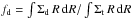 is constant with radius.
With this assumptions it is possible to solve Eqs. (5) and (6) for both
the gas density Σg and the mass inflow rate dMinfl/
dt. In particular, in the inner region
Racc ≤
R ≤ RBH where the BH
dominates the potential Φ
in Eq. (5), Eq. (6) yields 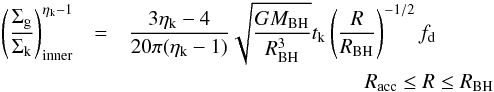 (A.1)while
in the outer region RBH ≤ R ≤
R0, where the potential
Φ is dominated by the
disk, the same equations yield
(A.1)while
in the outer region RBH ≤ R ≤
R0, where the potential
Φ is dominated by the
disk, the same equations yield 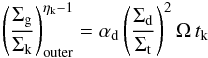 with
with
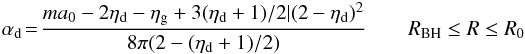 (A.2)where
![Mathematical equation: \hbox{$\Omega=\Big[G\,2\pi\,\int_0^R (\Sigma_{\rm d}+\Sigma_b)\,R\,{\rm d}R/R^3\Big]^{1/2}$}](/articles/aa/full_html/2014/09/aa24217-14/aa24217-14-eq289.png) is the angular velocity of the disk.
is the angular velocity of the disk.
Appendix A.3: The boundary conditions
To compute the accretion flow in the inner region Racc ≤ R ≤
RBH, we can use Eq. (A.1) to solve Eq. (6). However, the two density profiles in
Eqs. (A.1) and (A.2) are not matched to ensure a
continuous mass flux at the boundaries RBH and R0. In
principle, one could impose a continuity condition for such equations at all times.
Since the boundaries move as accretion proceeds, this would require a detailed
treatment following the dynamical evolution of the boundaries and of the mass flux
across them. Following HQ11, we adopt a simplified approach by we keeping the density
profiles in Eqs. (A.1) and (A.2), and we impose the mass conservation
directly in Eqs. (6). Thus, we write
the latter as 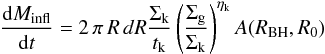 (A.3)where
A(RBH,R0)
expresses the proper boundary conditions, i.e., the mass conservation across the
boundaries RBH and R0. To
compute such a quantity, we note that the mass accreted into the inner region
(Racc ≤
R ≤ RBH) must equal
the disk mass that has flown across RBH. We indicate with
ΔMg the mass inside the boundary
RBH computed after integrating Eq.
(A.1), and with A(RBH,R0)ΔMg
the actual mass accreted in the inner region after matching with it with the mass
flown from the disk. In a time interval Δt, we must have
(A.3)where
A(RBH,R0)
expresses the proper boundary conditions, i.e., the mass conservation across the
boundaries RBH and R0. To
compute such a quantity, we note that the mass accreted into the inner region
(Racc ≤
R ≤ RBH) must equal
the disk mass that has flown across RBH. We indicate with
ΔMg the mass inside the boundary
RBH computed after integrating Eq.
(A.1), and with A(RBH,R0)ΔMg
the actual mass accreted in the inner region after matching with it with the mass
flown from the disk. In a time interval Δt, we must have
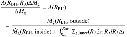 (A.4)We
must have Ṁg(RBH,outside)
=
Ṁg(RBH,inside).
Estimating exactly such a quantity would require a dynamical description of the
variation of the boundary with time and of the mass flux across it. However, a simple
– though approximate – estimate of such a quantity can be obtained by computing it as
the mass lost from a disk during Δt (divided by Δt). This can be
obtained after integrating the disk density profile A.2 extrapolated down to R = 0, so that
(A.4)We
must have Ṁg(RBH,outside)
=
Ṁg(RBH,inside).
Estimating exactly such a quantity would require a dynamical description of the
variation of the boundary with time and of the mass flux across it. However, a simple
– though approximate – estimate of such a quantity can be obtained by computing it as
the mass lost from a disk during Δt (divided by Δt). This can be
obtained after integrating the disk density profile A.2 extrapolated down to R = 0, so that
 . The quantity
B(R0) is the
normalization corresponding to the boundary condition at the galactic scale
R0, which ensures that the mass flux
outside the boundary R0 matches with that in the region
RBH ≤
R ≤ R0. We then
obtain
. The quantity
B(R0) is the
normalization corresponding to the boundary condition at the galactic scale
R0, which ensures that the mass flux
outside the boundary R0 matches with that in the region
RBH ≤
R ≤ R0. We then
obtain 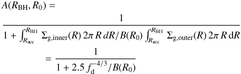 (A.5)where
the last equality follows after performing the integrals over Σg,inner and
Σg,outer given in Eqs. (A.1) and (A.2). The quantity A(RBH,R0)
acts like a suppression factor; when the mass inflow obtained using the (unmatched)
density distributions (A.1) and (A.2) yields an inflow rate that
exceeds the gas mass actually available from the disk at the
position RBH, it suppresses the mass flux so as
to maintain it lower or equal to this mass. In fact, for high values of
ΔMg(outside,RBH)
we get A(RBH,R0)
= 1. No suppression is needed since the disk mass available from
the disk is high.
(A.5)where
the last equality follows after performing the integrals over Σg,inner and
Σg,outer given in Eqs. (A.1) and (A.2). The quantity A(RBH,R0)
acts like a suppression factor; when the mass inflow obtained using the (unmatched)
density distributions (A.1) and (A.2) yields an inflow rate that
exceeds the gas mass actually available from the disk at the
position RBH, it suppresses the mass flux so as
to maintain it lower or equal to this mass. In fact, for high values of
ΔMg(outside,RBH)
we get A(RBH,R0)
= 1. No suppression is needed since the disk mass available from
the disk is high.
The quantity B(R0) in Eq. (A.3) can be obtained by iterating the same
mass-matching procedure exactly, but applying it to the outer boundary R0. In terms
of the disk mass Md(R0)
within R0 and of the corresponding gas mass
Mg(R0) =
fgasMd(R0),
the result reads as 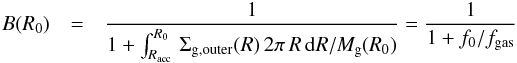 with
with
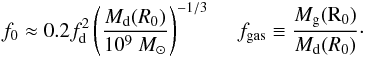 (A.6)The
physical meaning of the boundary factor B(R0) is to match
the gas available in the galactic disk (given by the semi-analytic model) with the gas
corresponding to the profile Σg inside R0. In the original HQ11 model, the
gas density profile Σg in the external region has a slightly higher
normalization to interpolate between the marginal and the strong orbit crossing
regimes; however, when such a factor is included, its effects on Eqs. (A.6) and (A.5) balance, leaving our results unchanged.
(A.6)The
physical meaning of the boundary factor B(R0) is to match
the gas available in the galactic disk (given by the semi-analytic model) with the gas
corresponding to the profile Σg inside R0. In the original HQ11 model, the
gas density profile Σg in the external region has a slightly higher
normalization to interpolate between the marginal and the strong orbit crossing
regimes; however, when such a factor is included, its effects on Eqs. (A.6) and (A.5) balance, leaving our results unchanged.
Appendix A.4: The BH inflow rate
We now proceed to solve Eq. (A.3) to
derive the mass inflow rate Minfl close to the inner bound
Racc. HQ11 first consider Eq. (6) in a ring close to Racc and
small enough that the surface density Σg can be considered to be constant. This yields
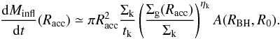 (A.7)After substituting
Eq. (A.1) computed ad the inner radius
Racc the above equation reads
(A.7)After substituting
Eq. (A.1) computed ad the inner radius
Racc the above equation reads
![Mathematical equation: \appendix \setcounter{section}{1} \begin{eqnarray} \label{intern_inflow} \frac{{\rm d}M_ {\rm BH}}{{\rm d}t} &&\equiv \frac{{\rm d}M_ {\rm infl} }{{\rm d}t} (R_{\rm acc}) = \pi \Sigma_{\rm k} t_{\rm k}^{\frac{1}{\eta_{\rm k}-1}} \left(\dfrac{R_{\rm acc}}{R_{\rm BH}} \right)^{{3\eta_{\rm k}-4 \over 2(\eta_{\rm k}-1)}} \nonumber\\ &&\quad \times R_{\rm BH}^2 \left[\dfrac{3 \eta_{\rm k} - 4}{20 \pi (\eta_{\rm k}-1)} \left(\frac{G M_{\rm BH}}{R_{\rm BH}^3}\right)^{\frac{1}{2}}f_{\rm d}\right]^{\frac{\eta_{\rm k}}{\eta_{\rm k}-1}}\,A(R_{\rm BH},R_0). \end{eqnarray}](/articles/aa/full_html/2014/09/aa24217-14/aa24217-14-eq312.png) (A.8)Equation
(A.8) represents the mass inflow in
the inner region corresponding to the BH accretion rate. We can relate RBH to
MBH in terms of the disk mass within
RBH through the relation
Mt(RBH) ≃
MBH. The mass Mt is
computed as
(A.8)Equation
(A.8) represents the mass inflow in
the inner region corresponding to the BH accretion rate. We can relate RBH to
MBH in terms of the disk mass within
RBH through the relation
Mt(RBH) ≃
MBH. The mass Mt is
computed as 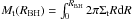 . For a power-law
profile Σt =
AΣtR−
ηd we can readily express
RBH as a function of Mt =
MBH to obtain
. For a power-law
profile Σt =
AΣtR−
ηd we can readily express
RBH as a function of Mt =
MBH to obtain 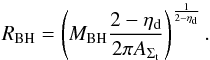 (A.9)Substituting in Eq.
(A.8) yields
(A.9)Substituting in Eq.
(A.8) yields ![Mathematical equation: \appendix \setcounter{section}{1} \begin{eqnarray} \label{intern_inflow1} \frac{{\rm d}M_ {\rm BH}}{{\rm d}t} &=& \pi \Sigma_{\rm k} t_{\rm k}^{\frac{1}{\eta_{\rm k}-1}} \Bigg[\dfrac{3 \eta_{\rm k} - 4}{20 \pi (\eta_{\rm k}-1)}\, G ^{\frac{1}{2}} \Bigg]^{\frac{\eta_{\rm k}}{\eta_{\rm k}-1}} \left(\frac{R_{\rm acc}}{R_{\rm BH}} \right)^{3\eta_{\rm k}-4 \over 2(\eta_{\rm k}-1)} \nonumber\\ &&\quad \times M_{\rm BH}^{3\eta_{\rm k}-4-\eta_{\rm k}\eta_{\rm d}\over 2\,(\eta_{\rm k}-1)\,(2-\eta_{\rm d})} f_{\rm d}^{\frac{\eta_{\rm k}}{\eta_{\rm k}-1}}\,\left(\dfrac{2 - \eta_{\rm d}}{2 \pi A_{\Sigma_{\rm t}}}\right)^{\frac{\eta_{\rm k}-4}{2(\eta_{\rm k}-1)(2-\eta_{\rm d})}}\,A(R_{\rm BH},R_0). \end{eqnarray}](/articles/aa/full_html/2014/09/aa24217-14/aa24217-14-eq319.png) (A.10)We
are now interested in expressing Eq. (A.8) using physical quantities evaluated far from the very central region,
at galactic scales R =
R0 ~ 102−103
pc, in order to derive the BH accretion rate from quantities computed from our
semi-analytic galaxy formation model. To this aim, we note that, for any disk profile
Σd, it is
possible to combine R0 and the associated enclosed disk
mass
(A.10)We
are now interested in expressing Eq. (A.8) using physical quantities evaluated far from the very central region,
at galactic scales R =
R0 ~ 102−103
pc, in order to derive the BH accretion rate from quantities computed from our
semi-analytic galaxy formation model. To this aim, we note that, for any disk profile
Σd, it is
possible to combine R0 and the associated enclosed disk
mass 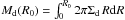 to
yield convenient constant quantities. In particular for a power-law profile, after
some algebra, the last two factors in Eq. (A.10) can be recast as
to
yield convenient constant quantities. In particular for a power-law profile, after
some algebra, the last two factors in Eq. (A.10) can be recast as 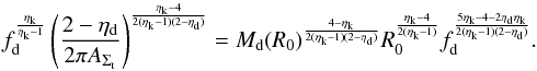 (A.11)After substituting in
Eq. (A.10) this reads as
(A.11)After substituting in
Eq. (A.10) this reads as ![Mathematical equation: \appendix \setcounter{section}{1} \begin{eqnarray} \label{intern_inflow2} &&\frac{{\rm d}M_ {\rm BH}}{{\rm d}t} = \pi \Sigma_{\rm k} t_{\rm k}^{\frac{1}{\eta_{\rm k}-1}} \left[\dfrac{3 \eta_{\rm k} - 4}{20 \pi (\eta_{\rm k}-1)}\, G ^{\frac{1}{2}} \right]^{\frac{\eta_{\rm k}}{\eta_{\rm k}-1}} \left(\frac{R_{\rm acc}}{R_{\rm BH}} \right)^{3\eta_{\rm k}-4 \over 2(\eta_{\rm k}-1)} \nonumber\\ &&\hspace*{3mm} \times M_{\rm BH}^{3\eta_{\rm k}-4-\eta_{\rm k}\eta_{\rm d}\over 2\,(\eta_{\rm k}-1)\,(2-\eta_{\rm d})} M_{\rm d}(R_0)^{\frac{4-\eta_{\rm k}}{2(\eta_{\rm k}-1)(2-\eta_{\rm d})}} R_0^{\frac{\eta_{\rm k}-4}{2(\eta_{\rm k}-1)}} f_{\rm d}^{\frac{5\eta_{\rm k}-4-2\eta_{\rm d}\eta_{\rm k}}{2(\eta_{\rm k}-1)(2-\eta_{\rm d})}} \,A(R_{\rm BH},R_0). \end{eqnarray}](/articles/aa/full_html/2014/09/aa24217-14/aa24217-14-eq324.png) (A.12)We
can express the above equation in physical units, which yields
(A.12)We
can express the above equation in physical units, which yields 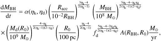 (A.13)where
we have gathered all constant terms into the normalization
(A.13)where
we have gathered all constant terms into the normalization  (A.14)The above expression
is the BH accretion rate for generic power-law surface density profiles. After
assuming a power law index ηd = 1 / 2 for the
gas surface density profile and an index ηk = 7 / 4 for the
Kennicut-Schmidt star formation law, the above equation yields Eq. (9) in the main
text and a normalization α(ηk,ηd)
= 0.18. As noted by HQ11, assuming different values for
ηd and ηk has only
a minor effect on the exponents in Eq. (A.13), but has a significant impact on α(ηk,ηd).
For example, changing the ηk to the value ηk = 3 /
2 yields α(ηk,ηd)
= 3.17. In the main text, we assume a reference value for
α(ηk,ηd)
= 10 to investigate the maximal contribution of
the DI mode to the evolution of the AGN population.
(A.14)The above expression
is the BH accretion rate for generic power-law surface density profiles. After
assuming a power law index ηd = 1 / 2 for the
gas surface density profile and an index ηk = 7 / 4 for the
Kennicut-Schmidt star formation law, the above equation yields Eq. (9) in the main
text and a normalization α(ηk,ηd)
= 0.18. As noted by HQ11, assuming different values for
ηd and ηk has only
a minor effect on the exponents in Eq. (A.13), but has a significant impact on α(ηk,ηd).
For example, changing the ηk to the value ηk = 3 /
2 yields α(ηk,ηd)
= 3.17. In the main text, we assume a reference value for
α(ηk,ηd)
= 10 to investigate the maximal contribution of
the DI mode to the evolution of the AGN population.
Appendix A.5: The nuclear star formation rate
The contribution to the star formation rate can be calculated integrating star
formation surface density rate  over the region of interest. The latter is related to the gas surface density by the
Schmidt-Kennicut law
over the region of interest. The latter is related to the gas surface density by the
Schmidt-Kennicut law  .
For the inner region, Σg is described by Eq. (A.1). Since all the terms in Eq. (A.1) are constant but the radius, we obtain
.
For the inner region, Σg is described by Eq. (A.1). Since all the terms in Eq. (A.1) are constant but the radius, we obtain  (A.15)The
normalization can be estimated considering the value that the star formation rate
assumes in R =
Racc. This can be done easily since
the mass inflow in R =
Racc is strictly related to star
formation surface density rate by Eq. (6) and gives
(A.15)The
normalization can be estimated considering the value that the star formation rate
assumes in R =
Racc. This can be done easily since
the mass inflow in R =
Racc is strictly related to star
formation surface density rate by Eq. (6) and gives  . Thus, the star formation
surface density rate in the inner region is equal to
. Thus, the star formation
surface density rate in the inner region is equal to  (A.16)The
contribution to the star formation rate in the inner region is then obtained by
integrating (A.16) from
Racc to RBH:
(A.16)The
contribution to the star formation rate in the inner region is then obtained by
integrating (A.16) from
Racc to RBH:
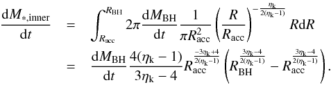 (A.17)For
the fiducial model, assuming ηk = 7 / 4 and
Racc ≃
10-2RBH, we obtain
(A.17)For
the fiducial model, assuming ηk = 7 / 4 and
Racc ≃
10-2RBH, we obtain
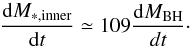 (A.18)The same
calculations can be performed for the outer region using the corresponding
(A.18)The same
calculations can be performed for the outer region using the corresponding
 ;
here the scaling and the exponent αd are given in Eq. (A.2). This yields
;
here the scaling and the exponent αd are given in Eq. (A.2). This yields 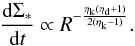 (A.19)The normalization can
be computed imposing continuity between the inner and the outer region. Using Eq.
(A.16)
(A.19)The normalization can
be computed imposing continuity between the inner and the outer region. Using Eq.
(A.16) 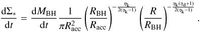 (A.20)Integrating Eq.
(A.20) from RBH to
R0, we obtain the star formation rate
in the outer region for the fiducial model:
(A.20)Integrating Eq.
(A.20) from RBH to
R0, we obtain the star formation rate
in the outer region for the fiducial model: 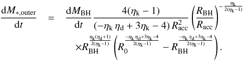 (A.21)Assuming
ηk = 7
/ 4, ηd = 1 / 2, and
Racc ≃
10-2RBH, we obtain
(A.21)Assuming
ηk = 7
/ 4, ηd = 1 / 2, and
Racc ≃
10-2RBH, we obtain
 (A.22)
Appendix B: Black hole accretion rate and nuclear star formation rate from disk instabilities: the case of exponential surface density profiles
Here we follow the same procedure as adopted in Appendix A, changing only the surface
density profile (and the corresponding potential) of the galactic disk. In particular,
we consider a thin disk whose density profile is described by the following
exponential-law: 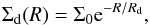 (B.1)where
Rd is the exponential length of the disk
and its order a few kpc. The potential associated to the disk is (Binney &
Tremaine 1987)
(B.1)where
Rd is the exponential length of the disk
and its order a few kpc. The potential associated to the disk is (Binney &
Tremaine 1987)
![Mathematical equation: \appendix \setcounter{section}{2} \begin{eqnarray} \Phi(R)=-\pi G \Sigma_0R\left[I_0(y)K_1(y)-I_1(y)K_0(y)\right] \end{eqnarray}](/articles/aa/full_html/2014/09/aa24217-14/aa24217-14-eq349.png) (B.2)where
y ≡
R/
2Rd and In, Kn are the modified
Bessel function of first and second kinds. Since both the disk and the bulge exponential
length are much greater than scales of our interest, we can use the asymptotic form for
the modified Bessel function; as a result, we obtain
(B.2)where
y ≡
R/
2Rd and In, Kn are the modified
Bessel function of first and second kinds. Since both the disk and the bulge exponential
length are much greater than scales of our interest, we can use the asymptotic form for
the modified Bessel function; as a result, we obtain 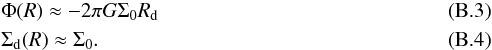 We
note that in this case the disk surface density and the potential are computed
self-consistently, at variance with the previous case where we assumed a WKB form for
the potential and a power-law form for the surface density.
We
note that in this case the disk surface density and the potential are computed
self-consistently, at variance with the previous case where we assumed a WKB form for
the potential and a power-law form for the surface density.
Following the same procedure as adopted in Appendix A, we consider two regions: an outer region where the potential is dominated by the disk, and an inner region where the BH gravity is dominant. The radius RBH ~ 10 pc marks the separations between the two regions, while the scale Racc ~ 0.1 pc corresponds to the inner bound of the innermost regions where we want to compute the BH accretion rate. The potential of the disk is only needed to calculate the analytic expression for Σg in the outer region, where the BH does not dominate the potential.
In the inner region, the potential is dominated by the BH, and the computation of the BH accretion rate follows the lines shown in Appendix A exactly, changing only the scaling of the disk radial profile by adopting ηd = 0, to achieve a constant Σd as given by Eq. (B.4). Thus, the BH accretion rate is given by the same Eq. (A.13) with ηd = 0. However, the boundary condition A(RBH,R0) is different from Appendix A, since it depends on the gas surface density Σg,outer in the region R>RBH where the potential and the surface densities need to be recomputed (see Eqs. (A.5) and (A.6)). Also, the contribution to the nuclear star formation from such a region R>RBH has to be recomputed, since it also depends on Σg,outer.
To computeΣg,outer in the outer region we start
from the perturbed potential in the outer region
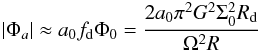 (B.5)with
a0 ~
0.3 and m
= 2, motivated by simulations. Substituting the above expression into
Eq. (5) we obtain for the outer region
(from RBH to R0)
(B.5)with
a0 ~
0.3 and m
= 2, motivated by simulations. Substituting the above expression into
Eq. (5) we obtain for the outer region
(from RBH to R0)
 (B.6)with
 (B.7)where
we have used the relation Ω2R = G∫2
π ΣtR
dR, and Σt is the total (disk + bulge) surface density profiles
(see Appendix A). Substituting such an expression in Eq. (6) yields
(B.7)where
we have used the relation Ω2R = G∫2
π ΣtR
dR, and Σt is the total (disk + bulge) surface density profiles
(see Appendix A). Substituting such an expression in Eq. (6) yields  (B.8)That is the
equation for Σg
in the outer region RBH ≤ R ≤
R0 and the counterpart of Eq. (A.2) in the case of an exponential disk
surface density profile; in the inner region Racc ≤ R ≤
RBH, the analytic expression for
Σg is the same
as Eq. (A.1), since this region is
dominated by BH potential. We can now recompute the boundary conditions A(RBH,R0)
and B(R0). To this aim,
we use Eqs. (A.5) and (A.6), but adopting the expression in Eq.
(B.8) for the gas surface density in
the outer region Σg,outer. This yields
(B.8)That is the
equation for Σg
in the outer region RBH ≤ R ≤
R0 and the counterpart of Eq. (A.2) in the case of an exponential disk
surface density profile; in the inner region Racc ≤ R ≤
RBH, the analytic expression for
Σg is the same
as Eq. (A.1), since this region is
dominated by BH potential. We can now recompute the boundary conditions A(RBH,R0)
and B(R0). To this aim,
we use Eqs. (A.5) and (A.6), but adopting the expression in Eq.
(B.8) for the gas surface density in
the outer region Σg,outer. This yields
 (B.9)In
practice, the right-hand term in the parenthesis is extremely small, owing to the choice
of ηk, ηd (
ηd ~
0 since Σ0 is almost constant) and to the factor Rd/RBH,
so that the above expression for the case of an exponential disk always yields
A(RBH,R0)
≈ 1, independently of the outer boundary condition, which anyway
reads (in the case ηk = 7 / 4)
(B.9)In
practice, the right-hand term in the parenthesis is extremely small, owing to the choice
of ηk, ηd (
ηd ~
0 since Σ0 is almost constant) and to the factor Rd/RBH,
so that the above expression for the case of an exponential disk always yields
A(RBH,R0)
≈ 1, independently of the outer boundary condition, which anyway
reads (in the case ηk = 7 / 4)
![Mathematical equation: \appendix \setcounter{section}{2} \begin{eqnarray} \label{div3} B(R_0) \approx \Bigg[ 1+26\,{f_0\over f_{\rm gas}} \Bigg({R_{\rm d} \over R_0 } \Bigg)^{4/3} \Bigg]^{-1} \end{eqnarray}](/articles/aa/full_html/2014/09/aa24217-14/aa24217-14-eq369.png) (B.10)where
f0 and fgas are those
given in Eq. (A.6). Thus, in the main
text, we adopt the excellent approximation A(RBH,R0)
= 1.
(B.10)where
f0 and fgas are those
given in Eq. (A.6). Thus, in the main
text, we adopt the excellent approximation A(RBH,R0)
= 1.
As for the nuclear star formation, the contribution from the inner region Racc ≤ R ≤ RBH is the same as given in Eq. (A.17), since in this region the potential is dominated
by the BH. In the outer region, we follow the procedure presented in Sect. A5, based on
the relation  ,
with the latter quantity taken from Eq. (B.8). This yields
,
with the latter quantity taken from Eq. (B.8). This yields 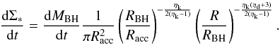 (B.11)Integrating Eq. (B.11) from RBH to
R0, we obtain
(B.11)Integrating Eq. (B.11) from RBH to
R0, we obtain
![Mathematical equation: \appendix \setcounter{section}{2} \begin{eqnarray} \dfrac{{\rm d}M_ {*,\rm outer}}{{\rm d}t} &=& \dfrac{{\rm d}M_ {\rm BH}}{{\rm d}t} \dfrac{4(\eta_{\rm k}-1)}{(-\eta_{\rm k} \, \eta_{\rm d} + \eta_{\rm k} -4 )\,R_{\rm acc}^2} \left(\dfrac{R_{\rm BH}}{R_{\rm acc}}\right)^{-\frac{\eta_{\rm k}}{2(\eta_{\rm k}-1)}}\nonumber\\[2mm] &&\quad \times R_{\rm BH}^{\frac{\eta_{\rm k}(\eta_{\rm d}+3)}{2(\eta_{\rm k}-1)}}\left(R_0^{\frac{- \eta_{\rm k} \, \eta_{\rm d} + \eta_{\rm k} -4}{2 ( \eta_{\rm k} -1)}}-R_{\rm BH}^{\frac{- \eta_{\rm k} \, \eta_{\rm d} + \eta_{\rm k} -4}{2 ( \eta_{\rm k} -1)}}\right). \end{eqnarray}](/articles/aa/full_html/2014/09/aa24217-14/aa24217-14-eq373.png) (B.12)Taking
ηk = 7
/ 4, ηd = 0, and R0 = 100 pc,
(B.12)Taking
ηk = 7
/ 4, ηd = 0, and R0 = 100 pc,
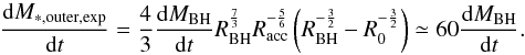 (B.13)At variance
with the case of power law profile given in Eq. (A.21), the star formation rate does not diverge with increasing
R0, due to the exponential decay of the
disk surface density.
(B.13)At variance
with the case of power law profile given in Eq. (A.21), the star formation rate does not diverge with increasing
R0, due to the exponential decay of the
disk surface density.
Acknowledgments
This work was supported by ASI/INAF contracts I/024/05/0 and I/009/10/0 and PRIN INAF 2011.
References
- Abazajian, K. N., Adelman-McCarthy, J. K., Agueros, M. A., et al. 2009, ApJS, 182, 543 [NASA ADS] [CrossRef] [Google Scholar]
- Adelman-McCarthy, J. K., Jennifer, K., Agüeron, M. A., et al. 2006, ApJS, 162, 38 [NASA ADS] [CrossRef] [Google Scholar]
- Aird, J., Nandra, K., Laird, E.S., et al. 2010, MNRAS, 401, 2531 [NASA ADS] [CrossRef] [Google Scholar]
- Aller, M. C., & Richstone, D. O. 2007, ApJ, 665, 120 [NASA ADS] [CrossRef] [Google Scholar]
- Alonso, M. S., Lambas, D. G., Tissera, P. B., & Coldwell, G. 2007, MNRAS, 375, 1017 [NASA ADS] [CrossRef] [Google Scholar]
- Anglés-Alcázar, D., Özel, F., & Davé, R. 2013, ApJ, 770, 5 [NASA ADS] [CrossRef] [Google Scholar]
- Anderson, C. S., Johnston, H. M., & Hunstead, R. W. 2013, MNRAS, 431, 3269 [NASA ADS] [CrossRef] [Google Scholar]
- Athanassoula, E. 1992, MNRAS, 259, 328 [NASA ADS] [CrossRef] [Google Scholar]
- Bahcall, J. N., Kirhakos, S., Saxe, D. H., & Schneider, D. P. 1997, ApJ, 479, 642 [NASA ADS] [CrossRef] [Google Scholar]
- Baldry, I. K., Glazebrook, K., Brinkmann, J., et al. 2004, ApJ, 600, 681 [NASA ADS] [CrossRef] [Google Scholar]
- Baldry, I. K., Driver, S. P., Loveday, J., et al. 2012, MNRAS, 421, 621 [NASA ADS] [Google Scholar]
- Bardeen, J. M., Bond, J. R., Kaiser, N., & Szalay, A. S. 1986, ApJ, 304, 15 [NASA ADS] [CrossRef] [Google Scholar]
- Barnes, J. E., & Hernquist, L. E. 1991, ApJ, 370, L65 [NASA ADS] [CrossRef] [Google Scholar]
- Baugh, C. M. 2006, Rep. Prog. Phys. 69, 3101 [NASA ADS] [CrossRef] [Google Scholar]
- Bennert, N., Canalizo, G., Jungwiert, B., et al. 2008, ApJ, 677, 846 [NASA ADS] [CrossRef] [Google Scholar]
- Benson, A. J., & Devereux, N. 2010, MNRAS, 402, 2321 [NASA ADS] [CrossRef] [Google Scholar]
- Binney, J., Tremaine, S. 1987, Galactic dynamics (Princeton: Princeton Univ. Press), 747 [Google Scholar]
- Bond, J. R., Cole, S., Efstathiou, G., & Kaiser, N. 1991, ApJ, 379, 440 [NASA ADS] [CrossRef] [Google Scholar]
- Bongiorno, A., Zamorani, G., Gavignaud, I., et al. 2007, A&A, 472, 443 [NASA ADS] [CrossRef] [EDP Sciences] [Google Scholar]
- Bouché, N., Cresci, G., Davies, R., et al. 2007, ApJ, 671, 303 [NASA ADS] [CrossRef] [Google Scholar]
- Bournaud, F., Combes, F., & Semelin, B. 2005, MNRAS, 364, L18 [Google Scholar]
- Bournaud, F., Elmegreen, B. G., & Elmegreen, D. M. 2007, ApJ, 670, 237 [Google Scholar]
- Bournaud, F., Dekel, A., Teyssier, R., et al. 2011, ApJ, 741, L33 [NASA ADS] [CrossRef] [Google Scholar]
- Bournaud, F., Juneau, S., Le Floc’h, E., et al. 2012, ApJ, 757, 81 [NASA ADS] [CrossRef] [Google Scholar]
- Bouwens, R. G., Illingworth, G. D., Franx, M., & Ford, H. 2007, ApJ, 670, 928 [NASA ADS] [CrossRef] [Google Scholar]
- Bouwens, R. J., Illingworth, G. D., Oesch, P. A, et al. 2011, ApJ, 737, 90 [NASA ADS] [CrossRef] [Google Scholar]
- Bower, R. G. 1991, MNRAS, 248, 332 [NASA ADS] [CrossRef] [Google Scholar]
- Bower, R. G., Benson, A. J., Malbon, R., et al. 2006, MNRAS, 370, 645 [NASA ADS] [CrossRef] [Google Scholar]
- Brusa, M., Civano, F., Comastri, A., et al. 2010, ApJ, 716, 348 [NASA ADS] [CrossRef] [Google Scholar]
- Bruzual, G., Charlot, S. 2003, MNRAS, 344, 1000 [NASA ADS] [CrossRef] [Google Scholar]
- Cappellari, M., Bacon, R., Bureau, M., et al. 2006, MNRAS, 366, 1126 [NASA ADS] [CrossRef] [Google Scholar]
- Cavaliere, A., & Vittorini, V. 2000, ApJ, 543, 599 [NASA ADS] [CrossRef] [Google Scholar]
- Ceverino, D., Bournaud, F., & Dekel, A. 2010, MNRAS, 404, 2151 [NASA ADS] [Google Scholar]
- Cirasuolo, M., McLure, R. J., Dunlop, J. S., et al. 2010, MNRAS, 401, 1166 [NASA ADS] [CrossRef] [Google Scholar]
- Cisternas, M., Jahnke, K., Inskip, K. J., et al. 2011, ApJ, 726, 57 [NASA ADS] [CrossRef] [Google Scholar]
- Civano, F., Brusa, M., Comastri, A., et al. 2011 ApJ, 741, 91 [NASA ADS] [CrossRef] [Google Scholar]
- Cole, S., Lacey, C. G., Baugh, C. M., & Frenk, C. S. 2000, MNRAS, 319, 168 [NASA ADS] [CrossRef] [Google Scholar]
- Combes, F., & Gerin, M. 1985, A&A, 150, 327 [NASA ADS] [Google Scholar]
- Combes, F., Baker, A. J., Schinnerer, E., et al. 2009, A&A, 503, 73 [NASA ADS] [CrossRef] [EDP Sciences] [Google Scholar]
- Croton, D. J., Springel, V., White, S. D. M., et al. 2006, MNRAS, 365, 11 [NASA ADS] [CrossRef] [Google Scholar]
- Cox, T. J., Dutta, S. N., Di Matteo, et al. 2006, ApJ, 650, 791 [NASA ADS] [CrossRef] [Google Scholar]
- Cox, T. J., Jonsson, P., Somerville, R. S., Primack, J. R., & Dekel, A. 2008, MNRAS, 384, 386 [NASA ADS] [CrossRef] [Google Scholar]
- Croom, S. M., Richards, G. T., Shanks, T., et al. 2009, MNRAS, 399, 1755 [NASA ADS] [CrossRef] [Google Scholar]
- Daddi, E., Elbaz, D., Walter, F., et al. 2010, ApJ, 714, L118 [Google Scholar]
- Darg, D. W., Kaviraj, S., Lintott, C. J., et al. 2010, MNRAS, 401, 1552 [NASA ADS] [CrossRef] [Google Scholar]
- Davies, R. I., SaAnchez, F. M.,Genzel, R., et al. 2007, ApJ, 671, 1388 [NASA ADS] [CrossRef] [Google Scholar]
- De Lucia, G., Fontanot, F., Wilman, D., & Monaco, P. 2011, MNRAS, 414, 1439 [NASA ADS] [CrossRef] [Google Scholar]
- de Vries, W. H., Morganti, R., Rottgering, H. J. A., et al. 2002, AJ, 123, 1784 [NASA ADS] [CrossRef] [Google Scholar]
- Disney, M. J., Boyce, P. J., Blades, J. C., et al. 1995, Nature, 376, 150 [NASA ADS] [CrossRef] [Google Scholar]
- Dotti, M., Ruszkowski, M., Paredi, L., et al. 2009, MNRAS, 396, 1640 [NASA ADS] [CrossRef] [Google Scholar]
- Drory, N., Bender, R., Feulner, G., et al. 2004, ApJ, 608, 742 [NASA ADS] [CrossRef] [Google Scholar]
- Ebrero, J., Carrera, F. J., Page, M. J., et al. 2009, A&A, 493, 55 [NASA ADS] [CrossRef] [EDP Sciences] [Google Scholar]
- Efstathiou, G., Lake, G., & Negroponte, J. 1982, MNRAS, 199, 1069 [NASA ADS] [CrossRef] [Google Scholar]
- Eisenhardt, P. R., Stern, D., Brodwin, M., et al. 2004, ApJS, 154, 48 [NASA ADS] [CrossRef] [Google Scholar]
- Eliche-Moral, M. C., Gonzalez-Garcia, A. C., Balcells, M., et al. 2008, in Formation and Evolution of Galaxy Disks, eds. J. G. Funes, & E. M. Corsini (San Francisco, CA: ASP), ASP Conf. Ser. 396, 359 [Google Scholar]
- Ellison, S. L., Patton, D. R., Mendel, J. T., & Scudder, J. M. 2011, MNRAS, 418, 2043 [NASA ADS] [CrossRef] [Google Scholar]
- Fanidakis, N., Baugh, C. M., Benson, A. J., et al. 2012, MNRAS, 419, 2797 [NASA ADS] [CrossRef] [Google Scholar]
- Ferrarese, L., & Merritt, D. 2000, ApJ, 539, L9 [NASA ADS] [CrossRef] [Google Scholar]
- Fiore, F., O’Dwyer, B., Del Zanna, G., et al. 2012, A&A, 537, 22 [Google Scholar]
- Fisher, D. B., Drory, N. 2011, ApJ, 733, L47 [NASA ADS] [CrossRef] [Google Scholar]
- Fontana, A., Salimbeni, S., Grazian, A., et al. 2006, A&A, 459, 745 [NASA ADS] [CrossRef] [EDP Sciences] [Google Scholar]
- Fontanot, F., Cristiani, S., Monaco, P., et al. 2007, A&A, 461, 39 [NASA ADS] [CrossRef] [EDP Sciences] [Google Scholar]
- Friedli, D., & Martinet, L. 1993, A&A, 277, 27 [NASA ADS] [Google Scholar]
- Gebhardt, K., Bender, R., Bower, G., et al. 2000, ApJ, 539, L13 [NASA ADS] [CrossRef] [Google Scholar]
- Genzel, R., Burkert, A., Bouché, N., et al. 2008, ApJ, 687, 59 [NASA ADS] [CrossRef] [Google Scholar]
- Genzel, R., Tacconi, L. J., Gracia-Carpio, J., et al. 2010, MNRAS, 407, 2091 [NASA ADS] [CrossRef] [Google Scholar]
- Giavalisco, M., Dickinson, M., Ferguson, H. C., et al. 2004, ApJ, 600, L103 [NASA ADS] [CrossRef] [Google Scholar]
- Glikman, E., Djorgovski, S. G., Stern, D., et al. 2011, ApJ, 728, L26 [NASA ADS] [CrossRef] [Google Scholar]
- Giallongo, E., Menci, N., Fiore, F., et al. 2012, ApJ, 755, 124 [NASA ADS] [CrossRef] [Google Scholar]
- Goldreich, P., & Lynden-Bell, D. 1965, MNRAS, 130, 97 [NASA ADS] [CrossRef] [Google Scholar]
- Goldreich, P., & Tremaine, S. 1980, ApJ, 241, 425 [NASA ADS] [CrossRef] [MathSciNet] [Google Scholar]
- Gonzalez Delgado, R. M., Arribas, S., Perez, E., & Heckman, T. 2002, ApJ, 579, 188 [NASA ADS] [CrossRef] [Google Scholar]
- Grogin, N. A., Conselice, C. J., Chatzichristou, E., et al. 2005, ApJ 627, L97 [NASA ADS] [CrossRef] [Google Scholar]
- Häring, N., & Rix, H.-W. 2004, ApJ, 604, L89 [NASA ADS] [CrossRef] [Google Scholar]
- Heller, C. H., & Shlosman, I. 1994, ApJ, 424, 84 [NASA ADS] [CrossRef] [Google Scholar]
- Hennawi, J. F., Myers, A. D., Shen, Y., et al. 2010, ApJ, 719, 1672 [NASA ADS] [CrossRef] [Google Scholar]
- Henriques, B. M. B., & Thomas, P. A. 2010, MNRAS, 403, 768 [NASA ADS] [CrossRef] [Google Scholar]
- Hernquist, L. 1989, Nature, 340, 687 [NASA ADS] [CrossRef] [Google Scholar]
- Hernquist, L., & Mihos, J. C. 1995, ApJ, 448, 41 [NASA ADS] [CrossRef] [Google Scholar]
- Hickox, R. C., Jones, C., Forman, W. R., et al. 2009, ApJ, 696, 891 [Google Scholar]
- Hicks, E. K. S., Davies, R. I., Malkan, M. A., et al. 2009, ApJ, 696, 448 [NASA ADS] [CrossRef] [Google Scholar]
- Hildebrandt, H., Pielorz, J., Erben, T., et al. 2009, A&A, 498, 725 [NASA ADS] [CrossRef] [EDP Sciences] [Google Scholar]
- Hirschmann, M., Somerville, R. S., Naab, T., & Burkert, A. 2012, MNRAS, 426, 237 [NASA ADS] [CrossRef] [Google Scholar]
- Hopkins, P. F., & Quataert, E. 2010, MNRAS, 407, 1529 [NASA ADS] [CrossRef] [Google Scholar]
- Hopkins, P. F., & Quataert, E. 2011, MNRAS, 411, 1027 (HQ11) [NASA ADS] [CrossRef] [Google Scholar]
- Hopkins, P. F., Richards, G. T., & Hernquist, L. 2007, ApJ, 654, 731 [NASA ADS] [CrossRef] [Google Scholar]
- Hopkins, P. H., Somerville, R. S., Cox, T. J., et al. 2009, MNRAS, 397, 802 [NASA ADS] [CrossRef] [Google Scholar]
- Hutchings, J. B. 1987, ApJ, 320, 122 [NASA ADS] [CrossRef] [Google Scholar]
- Jiang, L., Fan, X., Bian, F. et al. 2009, AJ, 138, 305 [NASA ADS] [CrossRef] [Google Scholar]
- Jogee, S. 2006, Lect. Notes Phys, 693, 143 [NASA ADS] [CrossRef] [Google Scholar]
- Jones, D. H., Peterson, B. A., Colless, M., & Saunders, W. 2006, MNRAS, 396, 535 [Google Scholar]
- Kaspi, S., Smith, P. S., Netzer, H., et al. 2000, ApJ, 533, 631 [NASA ADS] [CrossRef] [Google Scholar]
- Kauffmann, G., & Heckman, T. M. 2009, MNRAS, 397, 135 [NASA ADS] [CrossRef] [Google Scholar]
- Kauffmann, G., Heckman, T. M., Tremonti, C., et al. 2003, MNRAS, 346, 1055 [Google Scholar]
- Kenter, A., Murray, S. S., Forman, W. R., et al. 2005, ApJS, 161, 9 [NASA ADS] [CrossRef] [Google Scholar]
- Khochfar, S., & Silk, J. 2006, MNRAS, 370, 902 [NASA ADS] [CrossRef] [Google Scholar]
- King, I. 1962, AJ, 67, 471 [NASA ADS] [CrossRef] [Google Scholar]
- Kirhakos, S., Bahcall, J. N., Schneider, D. P., Kristian, J. 1999, ApJ, 520, 67 [NASA ADS] [CrossRef] [Google Scholar]
- Kocevski, D. D., Faber, S. M., Mozena, M., et al. 2012, ApJ, 744, 148 [NASA ADS] [CrossRef] [Google Scholar]
- Kollatschny, W., Reichstein, A., & Zetzl, M. 2012, A&A, 548, 37 [NASA ADS] [CrossRef] [EDP Sciences] [Google Scholar]
- Kollmeier, J. A., Oken, C. A., Kochanek, C. S., et al. 2006, ApJ, 648, 128 [NASA ADS] [CrossRef] [Google Scholar]
- Kormendy, J., & Richstone, D. 1995, ARA&A, 33, 581 [NASA ADS] [CrossRef] [Google Scholar]
- Koss, M., Mushotzky, R., Veilleux, S., & Winter, L. 2010, ApJ, 716, L125 [NASA ADS] [CrossRef] [Google Scholar]
- Lacey, C., & Cole, S. 1993, MNRAS, 262, 627 [NASA ADS] [CrossRef] [Google Scholar]
- La Franca, F., Fiore, F., Comastri, A., et al. 2005, ApJ, 635, 864 [NASA ADS] [CrossRef] [Google Scholar]
- Lamastra, A., Menci, N., Maiolino, R., Fiore, F., & Merloni, A. 2010, MNRAS, 405, 29 [NASA ADS] [Google Scholar]
- Lamastra, A., Menci, N., Fiore, F., & Santini, P. 2013a, A&A, 552, 44 [Google Scholar]
- Lamastra, A., Menci, N., Fiore, F., et al. 2013b, A&A, 559, A56 [NASA ADS] [CrossRef] [EDP Sciences] [Google Scholar]
- Li, C., & White, S. D. M. 2009, MNRAS, 398, 2177 [NASA ADS] [CrossRef] [Google Scholar]
- Li, C., Kauffmann, G., Wang, L., et al. 2006, MNRAS, 373, 457 [NASA ADS] [CrossRef] [Google Scholar]
- Lilly, S. J., Le Fevre, O., Renzini, A., et al. 2007, ApJS, 172, 70 [NASA ADS] [CrossRef] [Google Scholar]
- Lin, C. C., Yuan, C., & Shu, F. H. 1969, ApJ, 155, 721 [NASA ADS] [CrossRef] [Google Scholar]
- Lotz, J. M., Jonsson, P., Cox, T. J., et al. [Google Scholar]
- Lynden-Bell, D., & Kalnajs, A. J. 1972, MNRAS, 157, 1 [NASA ADS] [CrossRef] [Google Scholar]
- Maciejewski, W., & Sparke, L. S. 2000, MNRAS, 313, 745 [NASA ADS] [CrossRef] [Google Scholar]
- Mayer, L., Kazantzidis, S., Madau, P., et al. 2007, Science, 316, 1874 [NASA ADS] [CrossRef] [PubMed] [Google Scholar]
- Magorrian, J., Tremaine, S., Richstone, D., et al. 1998, AJ, 115, 2285 [NASA ADS] [CrossRef] [Google Scholar]
- Makino, J., & Hut, P. 1997, ApJ, 481, 83 [NASA ADS] [CrossRef] [Google Scholar]
- Marconi, A., & Hunt, L. K. 2003, ApJ, 589, L21 [NASA ADS] [CrossRef] [Google Scholar]
- Marconi, A., Risaliti, G., Gilli, R., et al. 2004, MNRAS, 351, 169 [NASA ADS] [CrossRef] [Google Scholar]
- McGurk, R. C., Max, C. E., Rosario, D. J., et al. 2011, ApJ, 738, 2 [NASA ADS] [CrossRef] [Google Scholar]
- Menci, N., Cavaliere, A., Fontana, A., et al. 2003, ApJ, 587, L63 [NASA ADS] [CrossRef] [Google Scholar]
- Menci, N., Cavaliere, A., Fontana, A., Giallongo, E., & Poli, F. 2004, ApJ, 604, 12 [NASA ADS] [CrossRef] [Google Scholar]
- Menci, N., Fontana, A., Giallongo, E., Grazian, A., & Salimbeni, S. 2006, ApJ, 647, 753 [NASA ADS] [CrossRef] [Google Scholar]
- Menci, N., Fiore, F., Puccetti, S., & Cavaliere, A. 2008, ApJ, 686, 219 [NASA ADS] [CrossRef] [Google Scholar]
- Mo, H. J, Mao, S., & White, S. D. M. 1998, MNRAS, 295, 319 [Google Scholar]
- Murray, S. S., Kenter, A., Forman, W. R., et al. 2005, ApJS, 161, 1 [NASA ADS] [CrossRef] [Google Scholar]
- Navarro, J. F., Frenk, C. S., & White, S. D. M. 1997, ApJ, 490, 493 [NASA ADS] [CrossRef] [Google Scholar]
- Netzer, H. 2009a, MNRAS, 399, 1907 [NASA ADS] [CrossRef] [Google Scholar]
- Netzer, H. 2009b, ApJ, 695, 793 [NASA ADS] [CrossRef] [Google Scholar]
- Ostriker, E. C., Shu, F. H., & Adams, F. C. 1992, ApJ, 399, 192 [NASA ADS] [CrossRef] [Google Scholar]
- Panter, B., Jimenez, R., Heavens, A. F., & Charlot, S. 2007, MNRAS, 378, 1150 [Google Scholar]
- Parry, O. H., Eke, V. R., & Frenk, C. S. 2009, MNRAS, 396, 1972 [NASA ADS] [CrossRef] [Google Scholar]
- Pierce, C. M., Lotz, J. M., Laird, E. S., et al. 2007, ApJ, 660, L19 [NASA ADS] [CrossRef] [Google Scholar]
- Reddy, N. A., & Steidel, C. S. 2009, ApJ, 692, 778 [NASA ADS] [CrossRef] [Google Scholar]
- Richards, G. T., Strauss, M. A., Fan, X., et al. 2006, ApJ, 131, 2766 [Google Scholar]
- Robertson, B., Cox, T. J., Hernquist, L., et al. 2006a, ApJ, 641, 21 [NASA ADS] [CrossRef] [Google Scholar]
- Robertson, B., Hernquist, L., Cox, T. J., et al. 2006b, ApJ, 641, 90 [NASA ADS] [CrossRef] [Google Scholar]
- Rodighiero, G., Daddi, E., Baronchelli, I., et al. 2011, ApJ, 739, L40 [NASA ADS] [CrossRef] [Google Scholar]
- Rogers, B., Ferreras, I., Kaviraj, S., Pasquali, A., & Sarzi, M. 2009, MNRAS, 399, 2172 [NASA ADS] [CrossRef] [Google Scholar]
- Rosario, D. J., Mozena, M., Wuyts, S., et al. 2013a, 763, 59 [Google Scholar]
- Rosario, D. J., Trakhtenbrot, B., Lutz, D., et al. 2013b, A&A, 560, A72 [NASA ADS] [CrossRef] [EDP Sciences] [Google Scholar]
- Salucci, P., Szuszkiewicz, E., Monaco, P., & Danese, L. 1999, MNRAS, 307, 637 [NASA ADS] [CrossRef] [Google Scholar]
- Sanders, D. B., & Mirabel, I. F. 1996, ARA&A, 34, 749 [NASA ADS] [CrossRef] [Google Scholar]
- Santini, P., Maiolino, R., Magnelli, B., et al. 2014, A&A, 562, 30 [Google Scholar]
- Saslaw, W. C. 1985, Gravitational Physics of Stellar and Galactic Systems (Cambridge: Cambridge Univ. Press) [Google Scholar]
- Schwarz, M. P. 1984, MNRAS, 209, 93 [NASA ADS] [CrossRef] [Google Scholar]
- Shankar, F., Weinberg, D. H., & Miralda-Escude, J. 2009, ApJ, 690, 20 [NASA ADS] [CrossRef] [Google Scholar]
- Shankar, F., Marulli, F., Mathur, S., Bernardi, M., & Bournaud, F. 2012, A&A, 540, A23 [NASA ADS] [CrossRef] [EDP Sciences] [Google Scholar]
- Shankar, F., Weinberg, D. H., & Miralda-Escude, J. 2013, MNRAS, 428, 421 [NASA ADS] [CrossRef] [Google Scholar]
- Shirasaki, Y., Tanaka, M., Ohishi, M., et al. 2011, PASJ, 63, 469 [NASA ADS] [Google Scholar]
- Shlosman, I., Frank, J., & Begelman, M. C. 1989, Nature, 338, 45 [NASA ADS] [CrossRef] [Google Scholar]
- Shu, F. H., Tremaine, S., Adams, F. C., & Ruden, S. P. 1990, ApJ, 358, 495 [NASA ADS] [CrossRef] [Google Scholar]
- Siana, B., Polletta, M., Smith, H. E., et al. 2008, ApJ, 675, 49 [NASA ADS] [CrossRef] [Google Scholar]
- Silverman, J. D., Lamareille, F., Maier, C., et al. 2009, ApJ, 696, 396 [NASA ADS] [CrossRef] [Google Scholar]
- Silverman, J. D., Kampczyk, P., Jahnke, K., et al. 2011, ApJ, 743, 2 [NASA ADS] [CrossRef] [Google Scholar]
- Somerville, R. S., & Primack, J. R. 1999, MNRAS, 310, 1087 [CrossRef] [Google Scholar]
- Somerville, R. S., Gilmore, R. C., Primack, J. R., & Dominguez, A. 2012, MNRAS, 423, 1992 [NASA ADS] [CrossRef] [Google Scholar]
- Spergel, D. N., Bean, R., Doré, O., et al. 2007, ApJS, 171, 377 [NASA ADS] [CrossRef] [Google Scholar]
- Stewart, K. R. 2009, in Galaxy Evolution: Emerging Insights and Future Challenges, eds. S. Jogee, I. Marinova, L. Hao, G. A. Blanc, ASP Conf. Ser. 419, 243 [Google Scholar]
- Storchi-Bergmann, T., González Delgado, R. M., Schmitt, H. R., Cid, F. R., & Heckman, T. 2001, in ASP Conf. Proc. 249, eds. J. H. Knapen, J. E. Beckman, I. Shlosman, & T. J. Mahoney, 259 (San Francisco: ASP) [Google Scholar]
- Taniguchi, Y. 1999, ApJ, 524, 65 [NASA ADS] [CrossRef] [Google Scholar]
- Taylor, J. E., Babul, A. 2001, ApJ, 559, 716 [NASA ADS] [CrossRef] [Google Scholar]
- Teyssier, R., Chapon, D., & Bournaud, F. 2010, ApJ, 720, L149 [NASA ADS] [CrossRef] [Google Scholar]
- Toomre, A. 1969, ApJ, 158, 899 [NASA ADS] [CrossRef] [Google Scholar]
- Trakhtenbrot, B., & Netzer, H. 2012, MNRAS, 427, 3081 [NASA ADS] [CrossRef] [Google Scholar]
- Treister, E., Schawinski, K., Urry, C. M., & Simmons, B. D. 2012, ApJ, 758, L39 [NASA ADS] [CrossRef] [Google Scholar]
- Tremaine, S., Gebhardt, K., Bender, R., et al. 2002, ApJ, 574, 740 [NASA ADS] [CrossRef] [Google Scholar]
- Trump, J. R., Impey, C. D., Elvis, M., et al. 2009, ApJ, 696, 1195 [NASA ADS] [CrossRef] [Google Scholar]
- Ueda, Y., et al. 2014, ApJ, in press [Google Scholar]
- van der Burg, R. F. J., Hildebrandt, H., & Erben, T. 2010, A&A, 523, 74 [Google Scholar]
- Villforth, C., Hamann, F., Rosario, D. J., et al. 2014, MNRAS, 439, 3342 [NASA ADS] [CrossRef] [Google Scholar]
- Villar-Martin, M., Tadhunter, C., Humphrey, A., et al. 2011, MNRAS, 416, 262 [NASA ADS] [Google Scholar]
- Villar-Martin, M, Cabrera Lavers, A., Bessiere, P., et al. 2012, MNRAS, 423, 80 [NASA ADS] [CrossRef] [Google Scholar]
- Woods, D. F., & Geller, M. J. 2007, AJ, 134, 527 [NASA ADS] [CrossRef] [Google Scholar]
- Yates, M. G., Miller, L., & Peacock, J. A. 1989, MNRAS, 240, 129 [NASA ADS] [CrossRef] [Google Scholar]
- York, D. G., Adelman, J., Anderson, J. E., et al. 2000, AJ, 120, 1579 [Google Scholar]
- Younger, J. D., Hopkins, P. F., Cox, T. J., & Hernquist, L. 2008, ApJ, 686, 815 [NASA ADS] [CrossRef] [Google Scholar]
- Yu, Q., & Tremaine, S. 2002, MNRAS, 335, 965 [NASA ADS] [CrossRef] [Google Scholar]
All Figures
|
Fig. 1 Left panel: predicted luminosity function at z ≤ 0.1 (in bj band, solid line) compared with observations from Jones et al. (2006). Central panel: predicted local stellar mass function (solid line) compared with data from Baldry et al. (2012, squares), Li & White (2009, triangles), Panter et al. (2007, circles), and Fontana et al. (2006, diamonds). Right panel: the contour plot shows the predicted relative fraction of bulge-to-total mass as a function of the galaxy stellar mass. This is compared with data from Fisher & Drory (2011). The corresponding distribution of B/T ratios (differential number of objects per B/T bin, normalized to the total number, solid line) is also compared with the SDSS data (Lackner & Gunn 2012, shaded histogram) in the rightmost panel, for galaxies in the magnitude range −24 ≤ Mr ≤ −17. |
| In the text | |
|
Fig. 2 Left panel: predicted local colour–magnitude relation. The colour code represents the number density of galaxies, normalized to the maximum value. Right panels: predicted colour distribution (differential number of objects per colour bin, normalized to the total number) for galaxies of different magnitudes (histograms) is compared with the data from the SDSS (Baldry et al. 2004, dots). |
| In the text | |
|
Fig. 3 Left panels: evolution of the K-band luminosity function predicted by the model (solid line) compared with the data from Cirasuolo et al. (2010, squares). Right panels: predicted evolution of the UV luminosity function (shaded region) compared with observed distribution of dropout galaxies. The shaded region encompasses the uncertainties due to the adopted extinction curve (Small Magellanic Cloud, Milky Way or Calzetti) In each redshift bin, the model galaxies have been selected according to the same selection criterium as adopted in the observations (see text). Data are taken from Reddy & Steidel (2009, dots), Bouwens et al. (2007, 2011, squares), and van der Burg et al. (2010, triangles). |
| In the text | |
|
Fig. 4 Predicted evolution of the AGN luminosity function in the UV band (at 1450 Å). Solid black lines refer to the IT scenario, and red solid lines to the DI model. We also plot variants of the DI model: dashed lines refer to the DI model computed with an exponential profile, while dotted lines to the DI model with increased star formation (see text). We compare with observed UV luminosity functions by Richards et al. (2006, solid squares), Croom et al. (2009, solid circles at z< 3 ), Siana et al. (2008, open squares), Bongiorno et al. (2007, open circles), Fontanot et al. (2007, solid diamonds), Glikman et al. (2011, big filled circles at z = 4.25), Jiang et al. (2009; solid squares at z ≥ 6). We also include luminosity functions from X-ray observations, converted to UV through the bolometric corrections in Marconi et al. (2004): the shaded region brackets the determinations derived in the X-ray band at z ≤ 2 by La Franca et al. (2005), Ebrero et al. (2009), Aird et al. (2010), while at higher redshifts we plot data from Fiore et al. (2012, penthagons), Brusa et al. (2010, triangle), Civano et al. (2011, green empty squares). |
| In the text | |
|
Fig. 5 Predicted evolution of the BH mass function in the IT scenario (solid black lines) and in the DI model (solid red line). The shaded region defines the spread in observational estimates obtained using different methods, as compiled by Shankar et al. (2009). |
| In the text | |
|
Fig. 6 Local MBH − M∗ relation for the IT model (left panels) and the DI model (right panels). Data points represent the observed local relation from Häring & Rix (2004, diamonds), and Marconi & Hunt (2003, squares, here M∗ is derived using the best-fitting virial relation of Cappellari et al. 2006); the colour code represents the fraction of AGN as a function of MBH for any given value of M∗, as indicated by the colour bar. We also show some of the paths in the MBH(t) − M∗(t) plane followed, during their evolution, by BHs (and by their host galaxies) reaching a final mass of MBH(z = 0) ≥ 109 M⊙. |
| In the text | |
|
Fig. 7 Predicted distribution of AGN in the LAGN − MBH plane for the IT (left) and DI (right) models is compared with data from Rosario et al. (2013a,b) in two redshift bins. The lines corresponding to Eddington ratio λ = 1, λ = 0.1 and λ = 0.01 are also indicated. |
| In the text | |
|
Fig. 8 Top left panel: predicted distributions of the Eddington ratio λ in the IT (solid black line) and DI (solid red line) scenarios for AGN with bolometric luminosity LAGN< 1046 erg s-1 at z ≤ 0.5. They are compared with different sets of data (see text for details): a sample of X-ray-selected AGN (dashed violet histogram), of IR-selected (dashed histogram) and Radio selected AGN (dotted histogram) from Hickox et al. (2009), and the sub-sample of X-ray and IR AGN from Kollmeier et al. (2006, dark green histogram) corresponding to z ≤ 0.5. Top right panel: as above, but for luminous AGN with LAGN> 1046 erg s-1 at z ≤ 1.2. The dashed histogram represents observational results from Kollmeier et al. (2006). Bottom left panel: as above, but for AGN with BH masses in the range 107 M⊙ ≤ MBH ≤ 08 M⊙. Here we compare with data from Kauffmann & Heckman (2009, histogram). Bottom right panel: fraction of AGN with high Eddington ratios λ ≥ 0.5 as a function of the AGN bolometric luminosity LAGN, at z = 2. As above, the solid black line corresponds to the IT mode and the solid red line to the DI case. The points are computed from the data by Rosario et al. (2013a,b) shown in Fig. 7. |
| In the text | |
Current usage metrics show cumulative count of Article Views (full-text article views including HTML views, PDF and ePub downloads, according to the available data) and Abstracts Views on Vision4Press platform.
Data correspond to usage on the plateform after 2015. The current usage metrics is available 48-96 hours after online publication and is updated daily on week days.
Initial download of the metrics may take a while.