| Issue |
A&A
Volume 569, September 2014
|
|
|---|---|---|
| Article Number | A10 | |
| Number of page(s) | 15 | |
| Section | Stellar structure and evolution | |
| DOI | https://doi.org/10.1051/0004-6361/201424144 | |
| Published online | 09 September 2014 | |
The environment of the fast rotating star Achernar⋆
III. Photospheric parameters revealed by the VLTI
1
Laboratoire Lagrange, UMR 7293, Université de Nice-Sophia Antipolis (UNS),
CNRS, Observatoire de la Côte d’Azur,
06300
Nice,
France
e-mail:
This email address is being protected from spambots. You need JavaScript enabled to view it.
2
LESIA, Observatoire de Paris, CNRS UMR 8109, UPMC, Université
Paris Diderot, 5 place Jules
Janssen, 92195
Meudon,
France
3
Instituto de Astronomia, Geofísica e Ciências Atmosféricas,
Universidade de São Paulo (USP), Rua do Matão 1226, Cidade Universitária,
05508-900
São Paulo,
Brazil
4
European Southern Observatory, Alonso de Córdova 3107, Casilla 19001
Santiago 19,
Chile
5
Univ. Grenoble Alpes, IPAG, 38000
Grenoble,
France
6
CNRS, IPAG, 38000
Grenoble,
France
7
Université de Toulouse, UPS-OMP, IRAP, 31028
Toulouse,
France
8
CNRS, IRAP, 14
avenue Édouard Belin, 31400
Toulouse,
France
9
Centre de Recherche en Astronomie, Astrophysique et Géophysique
(CRAAG), Route de l’Observatoire, BP 63, Bouzareah,
16340 Alger, Algérie
Received:
6
May
2014
Accepted:
6
July
2014
Abstract
Context. Rotation significantly impacts on the structure and life of stars. In phases of high rotation velocity (close to critical), the photospheric structure can be highly modified, and present in particular geometrical deformation (rotation flattening) and latitudinal-dependent flux (gravity darkening). The fastest known rotators among the nondegenerate stars close to the main sequence, Be stars, are key targets for studying the effects of fast rotation on stellar photospheres.
Aims. We seek to determine the purely photospheric parameters of Achernar based on observations recorded during an emission-free phase (normal B phase).
Methods. Several recent works proved that optical/IR long-baseline interferometry is the only technique able to sufficiently spatially resolve and measure photospheric parameters of fast rotating stars. We thus analyzed ESO-VLTI (PIONIER and AMBER) interferometric observations of Achernar to measure its photospheric parameters by fitting our physical model CHARRON using a Markov chain Monte Carlo method. This analysis was also complemented by spectroscopic, polarimetric, and photometric observations to investigate the status of the circumstellar environment of Achernar during the VLTI observations and to cross-check our model-fitting results.
Results. Based on VLTI observations that partially resolve Achernar, we simultaneously measured five photospheric parameters of a Be star for the first time: equatorial radius (equatorial angular diameter), equatorial rotation velocity, polar inclination, position angle of the rotation axis projected on the sky, and the gravity darkening β coefficient (effective temperature distribution). The close circumstellar environment of Achernar was also investigated based on contemporaneous polarimetry, spectroscopy, and interferometry, including image reconstruction. This analysis did not reveal any important circumstellar contribution, so that Achernar was essentially in a normal B phase at least from mid-2009 to end-2012, and the model parameters derived in this work provide a fair description of its photosphere. Finally, because Achernar is the flattest interferometrically resolved fast rotator to-date, the measured β and flattening, combined with values from previous works, provide a crucial test for a recently proposed gravity darkening model. This model offers a promising explanation to the fact that the measured β parameter decreases with flattening and shows significantly lower values than the classical prediction of von Zeipel.
Key words: stars: rotation / stars: individual: Achernar / methods: observational / methods: numerical / techniques: interferometric / techniques: high angular resolution
Based on observations performed at ESO, Chile under VLTI PIONIER and AMBER programme IDs 087.D-0150 and 084.D-0456.
© ESO, 2014
1. Introduction
The rapidly rotating Be star Achernar (α Eridani, HD 10144) is a key target in stellar physics for a deeper understanding of (1) the physical structure and evolution of fast rotators; and (2) the physical mechanism(s) connected with the Be phenomenon (e.g., episodic mass and angular momentum losses, disk formation and dissipation). It is thus crucial to determine a realistic model of Achernar’s photosphere by measuring its main relevant physical parameters such as radius, rotation velocity, temperature distribution (gravity darkening), mass, and inclination. Because it is the closest and brightest Be star in the sky, the photosphere of Achernar and its close vicinity can at least be partially resolved by modern high angular resolution instruments that can probe spatial scales ranging from ~1 to ~100 mas.
In particular, the ESO-Very Large Telescope Interferometer (VLTI; Haguenauer et al. 2010) instruments are well-adapted to this study. Observations performed in 2002 with the commissioning beam-combiner VLTI/VINCI revealed a strong apparent oblateness (rotational flattening) and suggested an extended structure that accounts for a few percent of the photospheric flux (Domiciano de Souza et al. 2003; Kervella & Domiciano de Souza 2006). This strong flattening could not be explained by the commonly adopted stellar rotation models, and two possibilities were proposed to account for it: differential rotation (Jackson et al. 2004), and a residual circumstellar disk (Carciofi et al. 2008). By studying the time variation of Hα line profiles, Vinicius et al. (2006) showed that a weak but measurable emission (relative to a reference spectra) was detectable at the epoch of the VLTI/VINCI observations; this supports the hypothesis of a residual disk.
In addition, direct high angular resolution imaging revealed a faint, lower-mass binary companion to the Be star, at angular separations of ~50 −300 mas (Kervella et al., in prep.; Kervella et al. 2008; Kervella & Domiciano de Souza 2007).
These works show that studying Achernar as a simple fast rotator to extract its photospheric parameters is a delicate task, since one has to consider its B⇆Be cycle as well as the possible influence of the binary companion. In this paper we seek to determine the purely photospheric parameters of Achernar based on a physical model of rapidly rotating stars and on VLTI observations recorded during a quiescent, emission-free phase (normal B phase).
The VLTI observations and data reduction are described in Sect. 2. In Sect. 3 we present a detailed investigation of the possible influence of a circumstellar disk and/or the binary companion on the interferometric observations. The adopted model and the photospheric parameters of Achernar measured from a model-fitting procedure are presented in Sects. 4 and 5. Deviations from the photospheric model and the photosphere vicinity of Achernar possibly revealed by the VLTI observations are investigated in Sect. 6, in particular using interferometric image reconstruction. Finally, the conclusions of this work are given in Sect. 7.
2. Interferometric observations and data reduction
2.1. VLTI/PIONIER
Near-infrared interferometric data of Achernar were obtained in 2011/Aug.-Sep. and 2012/Sep. with the PIONIER beam combiner (Le Bouquin et al. 2011) at the ESO-VLTI (Haguenauer et al. 2010). We used the largest quadruplet available with the Auxiliary Telescopes (AT) at that time (A1-G1-K0-I1) to resolve the stellar photosphere as much as possible. The resulting uv coverage is shown in Fig. 1. Depending on the night, the data were dispersed over three or seven spectral channels across the H band. Table 2 summarizes the log of observations.
The observations of Achernar were interspersed with interferometric calibrator stars to estimate the transfer function of the instrument. We selected these calibrators in the catalog by Cohen et al. (1999), adapted by Bordé et al. (2002), and in the JMMC Stellar Diameters Catalog1 (JSDC, Lafrasse et al. 2010) using the SearchCal tool developed by the JMMC2 (Bonneau et al. 2006). The main properties of the selected stars are listed in Table 1. We chose to use two types of calibrators: bright calibrators (HD 9362 and HD 12524) and fainter calibrators (HD 6793 and HD 187691). The bright calibrators provide a high photometric signal-to-noise ratio (S/N), and a very high precision on the calibration of the visibilities and closure phases. The fainter stars provide a cross-check of the adopted angular size of the bright calibrators and of their measured closure phases. Their small angular diameter results in a high fringe visibility (V ≈ 80%) and a very low systematic calibration uncertainty. We observed no deviation of the selected calibrators from central symmetry that might have been caused by binarity, for example.
Data were reduced and calibrated with the package pndrs (Le Bouquin et al. 2011). Each observation provides six squared visibilities V2 and four closure phases CP. This dataset is available upon request in the standard OIFITS format.
Interferometric calibrators used for the PIONIER observations of Achernar.
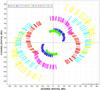 |
Fig. 1 uv coverage of VLTI/PIONIER observations of Achernar. The AT baselines used are identified with different colors. Image adapted from the OIFITSExplorer/JMMC tool. |
2.2. VLTI/AMBER
Domiciano de Souza et al. (2012a) described and analyzed VLTI/AMBER HR differential phase observations of Achernar around the Brγ line. The observations were recorded in 2009 (Oct. 25, Oct. 26, Oct. 30, and Nov. 1) with the high spectral resolution mode and using the FINITO fringe tracker. In this paper we reanalyze these AMBER differential phases together with the PIONIER data, since they were both taken during a diskless phase, as demonstrated in the next section.
3. Disk and companion status during the VLTI observations
The Be and binary nature of Achernar may imply temporal variabilities of observables with possible detectable spectro-interferometric signatures. It is thus important to determine which physical components should be included in the models to interpret VLTI observations from a given epoch. Indeed, Carciofi et al. (2008) showed that the presence of a residual circumstellar disk is a promising explanation of the strong flattening measured in the 2002 VLTI/VINCI observations (Domiciano de Souza et al. 2003). The presence of this residual disk is supported by a 2002 Hα profile that shows a weak but measurable emission superposed on the stronger photospheric absorption (Vinicius et al. 2006).
Based on our observations of Achernar (Kervella et al., in prep.), the binary companion was located close to apastron (separation ~200 − 300 mas) during the PIONIER observations, which is outside the field of view of this instrument. These observations were performed at the VLT instruments NACO and VISIR and are based on several high angular resolution imaging techniques such as direct imaging, lucky imaging, adaptive optics, and aperture masking. Although the stellar photosphere is not resolved by these observations, they allow one to follow the time evolution of the binary system by resolving both components at different orbital phases.
Concerning the possible influence of a Be circumstellar disk, a more thorough analysis is required as described below.
Log of VLTI/PIONIER observations of Achernar.
3.1. Search for polarimetric and spectroscopic signatures of a Be circumstellar disk
To investigate the presence and strength of a possible circumstellar disk during the VLTI (PIONIER and AMBER) observations (Sect. 2), we analyzed contemporaneous broadband polarimetry (B and V) and hydrogen line profiles (Hα and Hβ). These observations span from 2009 July to 2012 November.
Imaging polarimetry in the B and V bands was obtained using the IAGPOL polarimeter attached to the 0.6 m Boller & Chivens telescope at OPD/LNA3, Brazil. We used a CCD camera with a polarimetric module described by Magalhães et al. (1996), consisting of a rotating half-wave plate and a calcite prism placed in the telescope beam. A typical observation consists of 16 consecutive half-wave plate positions separated by 22.5°. In each observing run at least one polarized standard star HD 41117 or HD 187929 was observed to calibrate the observed position angle. Details of the data reduction can be found in Magalhães et al. (1984). A summary of our polarimetric data is presented in Table 3.
The IAGPOL data, shown in Fig. 2, exhibit values compatible with no intrinsic polarization, having a weighted average polarization of only 0.019 ± 0.012% during the observed period. This average is used in Sect. 3.2 as an upper limit to the polarization from a possible residual disk. This low polarization level contrasts with the measurements from a period of stellar activity in 2006, where the presence of circumstellar material lead to a polarization 10 times higher (up to 0.19% in B band), as shown by Carciofi et al. (2007). These authors also reported a clear spectroscopic signal with an Hα emission-to-continuum (E/C) ratio of ~1.06. The polarization values shown here also suggest no significant contribution from the interstellar medium to this quantity.
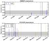 |
Fig. 2 Polarimetric observations at the epochs of ESO-VLTI AMBER and PIONIER data of Achernar analyzed in this work (vertical hatched bars). All the measurements are compatible with null/negligible polarization. The horizontal gray bars indicate the weighted average of the polarization: 0.019 ± 0.012%. Vertical lines correspond to epochs of Hα (dotted) and Hβ (dot-dashed) data observations with colors corresponding to the spectra shown in Fig. 3. The spectroscopic and polarimetric data are thus contemporaneous and embrace the interferometric observations in time. |
Summary of broadband polarization data that are contemporaneous to the VLTI observations.
Summary of spectroscopic data of Achernar that are contemporaneous to the VLTI observations.
In addition to the polarimetric data, Hα and Hβ spectra of Achernar contemporaneous to the VLTI observations were also analyzed in search for possible signatures of a circumstellar disk. We obtained seven spectra at OPD/LNA, using the Cassegrain spectrograph (ECass) with 600 groove mm-1 grating blazed at 6563 Å in first order, resulting in a reciprocal dispersion of 1.0 Å pixel-1. FEROS and HARPS spectra were also used to complement the OPD data. The spectroscopic observations are summarized in Table 4.
Following Rivinius et al. (2013), we adopted the FEROS spectra from early 2000 as a reference photospheric spectrum for Achernar. In Fig. 3 we plot the Hα and Hβ line profiles (top panels) and the difference profiles, computed as the difference between the observed profiles and the reference FEROS spectrum (bottom panels). All difference profiles are completely featureless, with difference values typically between − 0.012 and 0.012.
Thus, the polarimetric and spectroscopic data above suggest that the presence of a strong Be disk contemporaneous to the interferometric data can be discarded. In the following we quantify this assumption based on physical models of Be disks constrained by the observational limits imposed by the contemporaneous polarimetry (below 0.019 ± 0.012%) and spectroscopy (disk signatures below 0.012 in absolute values relative to a photospheric profile).
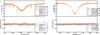 |
Fig. 3 Top: Hα (left) and Hβ (right) line profiles of Achernar at the epoch of interferometric observations. Bottom: difference in flux of the line profiles with respect to the reference FEROS spectrum from 2000 Jan. 11. This spectrum can be considered as a good approximation to the pure photospheric profile of Achernar (Rivinius et al. 2013). Whenever possible (enough spectral resolution) the telluric lines seen in some spectra have been removed before computing the differences. The horizontal shaded (gray) areas indicate the typical error on the difference profiles and also set a limit to them. |
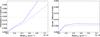 |
Fig. 4 Polarization in the B band (left) and standard deviation of difference Hα profile (right) as a function of disk-base density ρ0 for the residual disk models from Table 5 (model 1: full line; model 2: dashed line). The standard deviation is the root mean square of the disk model spectrum minus the pure photospheric profile. The horizontal dot-dashed lines represent the observational limits of average polarization and difference profile determined from observations performed at the epoch of interferometric observations, as explained in Sect. 3. While the measured Hα difference profile level does not impose a limit to ρ0, the measured average polarization sets a strict upper limit to this quantity: ρ0< 0.52 × 10⁻¹² g cm-3 for the thin-disk model and ρ0< 0.65 × 10⁻¹² g cm-3 for the thick-disk model. |
3.2. Residual disk
We investigate here whether the presence of a weak residual disk that is hard to detect from non-angularly resolved observations could still affect the interferometric observations of Achernar. This weak disk is constrained by the limits imposed by contemporaneous polarimetric and spectroscopic data determined in the previous section.
Using radiative transfer simulations from the HDUST code (Carciofi & Bjorkman 2006), we computed a grid of models based on our
previous grid used to investigate the 2002 phase of Achernar (Carciofi et al. 2008): a large and dense disk in hydrostatic equilibrium
(i.e., geometrically thin) and a smaller and more tenuous disk with enhanced scale height
(i.e., geometrically thick). We adopted a power-law radial density profile,  (1)where Req is the
stellar equatorial radius where the disk starts (inner disk radius), ρ0 is the
density of the disk at Req (density scale), and m is chosen as
3.5 corresponding to the
steady-stade regime of a viscous decretion disk (VDD) model (cf. Haubois et al. 2012, and references therein). To study the influence of
the disk on the different observables we varied ρ0 considering two sets of disk sizes
Rd and scale heights H0 at the inner
disk radius. Table 5 details the parameters of
these two sets of VDD models. In addition to these VDD models, we also used HDUST to
compute a reference ellipsoidal photospheric model of Achernar compatible with the more
physical photospheric model determined in Sect. 4.
(1)where Req is the
stellar equatorial radius where the disk starts (inner disk radius), ρ0 is the
density of the disk at Req (density scale), and m is chosen as
3.5 corresponding to the
steady-stade regime of a viscous decretion disk (VDD) model (cf. Haubois et al. 2012, and references therein). To study the influence of
the disk on the different observables we varied ρ0 considering two sets of disk sizes
Rd and scale heights H0 at the inner
disk radius. Table 5 details the parameters of
these two sets of VDD models. In addition to these VDD models, we also used HDUST to
compute a reference ellipsoidal photospheric model of Achernar compatible with the more
physical photospheric model determined in Sect. 4.
Parameters of the two geometrical configurations of the residual VDD models.
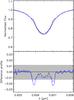 |
Fig. 5 Top: Hα line profile for the pure photospheric model (black solid line) and with a residual disk (VDD model) as defined in Table 5 and computed for the upper limit values of ρ0 (cf. Fig. 4): 0.52 × 10⁻¹² g cm-3 (thin disk; blue solid line) and 0.65 × 10⁻¹² g cm-3 (thick disk; blue dashed line). Bottom: the difference between the disk models relative to the photospheric model. The observational limit set to the difference profiles defined in Sect. 3 is indicated by the shaded (gray) region. |
The dependence of the polarimetric and spectroscopic observables on the density ρ0 for the two VDD models are shown in Fig. 4, where the quantities predicted from the models are compared with our observational constraints. By comparing the modeled and observed limits determined in Sect. 3 for the polarization and difference Hα spectra, we can set strict upper limits to ρ0: ρ0< 0.52 × 10⁻¹² g cm-3 (thin disk) and ρ0< 0.65 × 10⁻¹² g cm-3 (thick disk). As shown in Fig. 4, these limits are mainly imposed by the polarimetric data.
Figure 5 shows detailed a comparison of the VDD modeled Hα line profiles for these two ρ0 limits with the photospheric profile. As expected, the difference profiles have almost everywhere values within the ± 0.012 limit determined from the observed difference profiles (Sect. 3). Only at the wings of the Hα profiles the VDD models present some weak signatures differing slightly from the pure photospheric profile. This detailed investigation of Hα profiles combined with the results from Fig. 4 thus shows that the limits to ρ0 imposed by polarimetry are also reliable upper limits to hydrogen spectral lines.
By adopting these limits to ρ0 we now evaluate the signatures that a possible residual disk might have on our interferometric observations of Achernar. These evaluations are shown in Fig. 6, which compares the H band squared visibilities V2, and Brγ differential phases computed with the two VDD models (Table 5) with the expected values for the purely photospheric model. All deviations from the photospheric model are well within the typical observational errors on these interferometric quantities.
Therefore, in the following analysis we can safely rule out any effects of the known companion and of a significant residual disk around Achernar on our interferometric observations.
4. Achernar’s photospheric parameters from VLTI observations
Based on the results from the previous section we adopted a model of a fast rotating, single B star without circumstellar environment as a starting point to interpret the interferometric data of Achernar.
4.1. Photospheric model of fast-rotating stars
Most recent works describe the photospheric structure of rapidly rotating, nondegenerate, single stars of intermediate to high masses by adopting a Roche model (rigid rotation and mass concentrated in the stellar center) with a generalized form of the von Zeipel gravity darkening (von Zeipel 1924). We adopted this model since it has proven to well reproduce many distinct observables on rapid rotators (e.g., this work on Achernar and the cited references on other stars). Whether this is the only/best representation for their photospheres could be tested based on future and more precise observations.
Many codes exist that provide similar numerical implementations of this model, hereafter called the RVZ model. The reference numerical code for the RVZ model used here is the IDL-based program CHARRON (Code for High Angular Resolution of Rotating Objects in Nature). We present below a short description of CHARRON in the context of the present work. A more detailed description is given by Domiciano de Souza et al. (2012a,b, 2002).
The stellar photospheric shape follows Roche equipotential (gravitational plus
centrifugal),  (2)where θ is the colatitude,
M is the
stellar mass, and Req and Veq are the
equatorial radius and rotation velocity. Solving this cubic equation provides the
colatitude-dependent stellar radius R(θ).
(2)where θ is the colatitude,
M is the
stellar mass, and Req and Veq are the
equatorial radius and rotation velocity. Solving this cubic equation provides the
colatitude-dependent stellar radius R(θ).
Gravity darkening is considered by relating the local effective gravity geff(θ)(= | −
∇Ψ(θ)|) to the local effective temperature
Teff(θ) by,
 (3)where σ is the Stefan-Boltzmann
constant and β is the gravity-darkening coefficient, which is more
general than the β =
0.25 value from von Zeipel
(1924), but which is still assumed to be constant over the stellar surface. We
note that for the spectral type of Achernar we can neglect any radiative acceleration
effects since it is far from the Eddington limit. The proportionality constant
C can be
derived from stellar physical parameters such as mass and luminosity (e.g., Maeder & Meynet 2000) or related to a fixed
point on the photosphere (the stellar pole, for example). In this work, the constant
C and the
stellar luminosity L are related to the average effective temperature
(3)where σ is the Stefan-Boltzmann
constant and β is the gravity-darkening coefficient, which is more
general than the β =
0.25 value from von Zeipel
(1924), but which is still assumed to be constant over the stellar surface. We
note that for the spectral type of Achernar we can neglect any radiative acceleration
effects since it is far from the Eddington limit. The proportionality constant
C can be
derived from stellar physical parameters such as mass and luminosity (e.g., Maeder & Meynet 2000) or related to a fixed
point on the photosphere (the stellar pole, for example). In this work, the constant
C and the
stellar luminosity L are related to the average effective temperature
 over the total
stellar surface S⋆ (area of the Roche
photosphere),
over the total
stellar surface S⋆ (area of the Roche
photosphere),  (4) can be
directly related to the bolometric flux Fbol and to the mean angular diameter
(4) can be
directly related to the bolometric flux Fbol and to the mean angular diameter
 (diameter of spherical star having a surface area S⋆) by,
  (5)where
d is the
distance to the star.
(5)where
d is the
distance to the star.
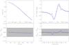 |
Fig. 6 Interferometric observables, squared visibilities V2 in the H band (left), and Brγ differential phases (right), computed for the pure photospheric model (black solid line) and for the two residual-disk models as defined in Table 5 at the upper limit values of ρ0 (cf. Fig. 4): 0.52 × 10⁻¹² g cm-3 (thin disk; blue solid line) and 0.65 × 10⁻¹² g cm-3 (thick disk; blue dashed line). The baseline position angle PA was chosen to lie along the stellar equator (cf. Sect. 4.2), so that the effects of the residual disk are maximized on these comparisons. The baseline length for the differential phase calculations roughly corresponds to half of the maximum available length. Bottom: the difference between the interferometric observables from the disk models relative to the photospheric model. The shaded areas correspond to the typical observational errors from our PIONIER and AMBER observations. These difference plots show that the disk contribution to the interferometric observables is only a small fraction of the observation errors even at the upper limit ρ0, discarding any detectable influence of a circumstellar disk on the present interferometric observations of Achernar. |
In our numerical implementation of the RVZ model the stellar surface is divided into a predefined grid with nearly identical surface area elements (typically ~50 000 surface elements). From Teff(θ) and geff(θ) defined in the above equations, a local specific intensity from a plane-parallel atmosphere I = I(geff,Teff,λ,μ) is associated with each surface element, where λ is the wavelength and μ is the cosine between the normal to the surface grid element and the line of sight (limb darkening is thus automatically included in the model). The local specific intensities I are interpolated from a grid of specific intensities that are pre-calculated using the spectral synthesis code SYNSPEC (Hubeny & Lanz 2011) and the ATLAS9 stellar atmosphere models (Kurucz 1979). For Achernar, we adopted atmosphere models with turbulent velocity of 2 km s-1 and solar abundance in agreement with its spectral type and short distance.
From the local specific intensities we obtained wavelengh-dependent intensity maps of the visible stellar surface at the chosen spectral domain and resolution, such as the image given in Fig. 11. The interferometric observables (e.g., squared visibilities, closure phases, differential phases) are then directly obtained from the Fourier transform of these sky-projected photospheric intensity maps, which for a given star in the sky also depend on its rotation-axis inclination angle i and on the position angle of its sky-projected rotation axis PArot (counted from north to east until the visible stellar pole).
Thus, the main input parameters of the photospheric RVZ model for fast rotators used to
interpret the interferometric observations of Achernar are M, Req,
Veq, β,
, i, PArot, and d.
 |
Fig. 7 Convergence of equatorial radius Req during the burn-in phase of the MCMC fit of the CHARRON RVZ model to the VLTI/PIONIER data using the emcee code (800 walkers and 200 iteration steps). |
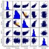 |
Fig. 8 Histogram distributions and two-by-two correlations for the free parameters (Req, Veq, i, β, and PArot) of the best-fit CHARRON RVZ model determined with the emcee code (800 walkers). The mean values and associated uncertainties obtained from these histograms are given in Table 6. The parameters do not show strong correlations in the region defined by the uncertainty around the mean values. The stronger correlation is shown by Veq and i, which roughly follow a curve of constant Veqsini (=260.3 km s-1), represented by the solid lines, with the circles indicating the mean values in the histograms. The rectangles cover the corresponding uncertainty ranges on Veq and i. |
Physical parameters of Achernar derived from the fit of the RVZ model (CHARRON code) to VLTI/PIONIER H band data using the MCMC method (emcee code).
4.2. Fitting of the CHARRON model to VLTI/PIONIER data with an MCMC method
We used the CHARRON model to constrain several photospheric parameters of Achernar from
the PIONIER observations (described in Sect. 2.1),
which consists of a homogenous data set obtained with the same beam-combiner instrument at
ESO-VLTI. To be compatible with the observations, the CHARRON intensity maps were
calculated over the H band with a spectral resolution of ~20−40. We note that in broadband observations, the effect of
bandwidth smearing (mixing of different spatial frequencies in a given wavelength bin) can
lead to a decrease of visibility contrast and should in principle be considered. However,
we checked that the bandwidth-smearing effect does not need to be considered in the
present analysis because (1) the squared visibilities are higher than 0.3−0.4, which minimizes this effect
(Kervella et al. 2003); and (2) the data span a
few wavelength bins over the H band so that the range of spatial frequencies mixed
is narrow. Based on results from previous works, M,
, and
d were
fixed to the following values:
-
M = 6.1 M⊙. Value from Harmanec (1988), previously adopted by Domiciano de Souza et al. (2012a). This mass also agrees (1) with the estimate from Jerzykiewicz & Molenda-Zakowicz (2000) (M = 6.22 ± 0.16 M⊙) based on evolutionary tracks; and (2) with the mass estimate from an on-going work on Achernar’s binary system (Kervella et al., in prep.);
-
 K. Value adopted by Domiciano de Souza et al. (2012a) following Vinicius et al. (2006). A critical discussion on
this value and comparisons with other works are presented in Sect. 5;
K. Value adopted by Domiciano de Souza et al. (2012a) following Vinicius et al. (2006). A critical discussion on
this value and comparisons with other works are presented in Sect. 5; -
d = 42.75 pc. We adopted the updated distance derived from the new reduction of the Hipparcos astrometric data and provided by van Leeuwen (2007).
The free parameters are thus Req, Veq, i, β, and PArot.
The model-fitting was performed using the emcee code (Foreman-Mackey et al. 2013), which is a Python implementation of a Markov chain Monte Carlo (MCMC) method proposed by Goodman & Weare (2010). This code has been recently used by Monnier et al. (2012) to interpret interferometric observations.
From a given likelihood function of the parameters, emcee provides histograms of the free
model parameters (samplings of the posterior probability) from which one can estimate the
best parameter values and associate uncertainties. In the present work, the measurement
errors on V2 and CP are all assumed to be
independent and normally distributed so that the likelihood function is proportional to
exp(−
χ2), where χ2 has its usual
definition and is composed of  (sum of
χ2 from the V2 and CP data,
respectively). To equally explore an homogenous range of initial values, we adopted
initial uniform distributions for the five free CHARRON parameters that cover a wide range
of physically consistent values.
(sum of
χ2 from the V2 and CP data,
respectively). To equally explore an homogenous range of initial values, we adopted
initial uniform distributions for the five free CHARRON parameters that cover a wide range
of physically consistent values.
The emcee algorithm explored the defined parameter space using 800 walkers in a 200 steps initial phase (burn-in) and 150 steps in the final phase, starting from the last state of the burn-in chain (for details of using the code see Foreman-Mackey et al. 2013). Convergence of the parameters distribution was typically attained within ≲100 steps during the burn-in phase (an example for Req is shown in the electronically available Fig. 7).
 |
Fig. 9 Top: squared visibilities V2 observed on Achernar (filled circles and error bars) and computed (opened squares) from the best-fit CHARRON model (Table 6) as a function of spatial frequency (left column) and baseline PA (right column). Bottom: V2 residuals from observations relative to the best-fit model in units of corresponding uncertainties. Vertical solid lines indicate the position angles of the visible (216.9° ≡ −143.1°) and hidden (16.9° = 216.9°−180°) stellar poles. The horizontal dotted lines delimit the ± 3σ region around zero (dashed line). |
The final histograms of the five free parameters and their two-by-two correlations are
shown in Fig. 8 (available electronically). The
best-fit values of the free parameters are the mean of these histograms. The uncertainties
on the parameters were defined as corresponding to a range enclosing ±34.15% of the parameter distribution
relative to the mean value (this corresponds to the commonly used rule for normal
distributions). The reduced χ2 of the best-fit model is
 (for
1777 degrees of freedom DOF and free free parameters).
(for
1777 degrees of freedom DOF and free free parameters).
Table 6 summarizes the best-fit parameter values and uncertainties measured on Achernar from the MCMC fit of CHARRON RVZ model to the VLTI/PIONIER data. Other derived stellar parameters are also given in the table. The V2 and CP corresponding to this best-fit model are plotted together with the observations in Figs. 9 and 10. The sky-projected intensity map of the visible stellar photosphere for this model is shown in Fig. 11.
As a completely independent check of the results above, we have also performed a Levenberg-Marquardt fit to the PIONIER data using a different RVZ model developed by one of us (A. Mérand). The best-fit parameter values obtained agree well (within the emcee error bars) with the values derived from the emcee fit of the CHARRON RVZ model.
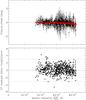 |
Fig. 10 Top: closure phases (CP) observed on Achernar and computed from
the best-fit CHARRON model (Table 6) as a
function of the spatial frequency (for the longest projected baseline
|

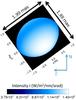 |
Fig. 11 Intensity map of Achernar corresponding to the best-fit of the CHARRON RVZ model to the VLTI/PIONIER H band observations. The spatial coordinates indicated in angular milliarcseconds (mas) units and also normalized to the equatorial radius Req = 9.16 R⊙. The complete list of the measured stellar parameters is given in Table 6. |
5. Discussion
5.1. Radius and angular diameter
Long-baseline interferometry is traditionally known to deliver stellar angular diameters (and radii, if distances are available). These size measurements are directly dependent on the chosen photospheric model and on how fairly this model can represent the stellar photosphere. As shown in Sect. 4, the stellar radius is a function of the co-latitude for fast rotators, and the apparent stellar photosphere is dependent on additional parameters such as gravity darkening, effective temperature, rotation velocity, and polar inclination (discussed in the following subsections).
As explained in the previous sections, the equatorial radius Req determined here (or more generally the photospheric R(θ)) is based on a physical model fitted to observations taken on a normal B phase of Achernar. As expected, the Req measured in this work is smaller than the previous results derived from VLTI/VINCI observations, obtained in an epoch with a small, but non-negligible influence of a residual disk (Domiciano de Souza et al. 2003; Kervella & Domiciano de Souza 2006; Carciofi et al. 2008).
We discuss the stellar size derived from the VLTI/AMBER observations by Domiciano de Souza et al. (2012a), we postpone the discussion to Sect. 5.5, where we consider the whole set of model parameters.
Considering the stellar size derived from the VLTI/AMBER observations by Domiciano de Souza et al. (2012a) in Sect. 5.5, where we consider the whole set of model parameters.
5.2. Photometry and effective temperature
The photometric magnitudes in the UBVJHK bands and the bolometric flux derived from the CHARRON best-fit model are compared with measurements reported in the literature in Table 7. We first note form the table that these observed magnitudes and bolometric fluxes show uncertainties and/or a dispersion of measured values of about 10% − 20%, which are at least partially caused by a combination of instrumental and intrinsic effects from the star. Indeed, Achernar is known to present multiple flux variabilities at time scales from hours to years, which are caused, for example, by pulsations (Goss et al. 2011), binarity (Kervella & Domiciano de Souza 2007), and the B⇆Be cycle (e.g., Vinicius et al. 2006). Thus, the observed magnitudes and bolometric flux should not be considered as tight constraints to the model-fitting, although they provide an important consistency check on the best-fit model parameters. Indeed, the modeled magnitudes and bolometric flux given in Table 7 agree with the observations within their uncertainties and/or dispersion of measured values.
Observed and modeled UBVJHK photometry and bolometric flux Fbol of Achernar.
By using Eq. (5) we can cross-check the
consistency between the adopted mean effective temperature
, the measured
bolometric flux Fbol, and the mean angular diameter
reported in Tables 6 and 7. From the Fbol provided by Code et al. (1976) and Nazé
(2009) one thus obtains  K and 14 703 K. We note that the temperature of
14 510 K estimated by Code et al. (1976) is somewhat lower than the value
estimated here because they considered the higher angular diameter (1.92 mas) reported by
Hanbury Brown et al. (1974), based on intensity
interferometry observations at the Narrabri Observatory. As expected, this diameter is
between the major and minor diameters derived in the present work. However, the
measurements from Hanbury Brown did not allow taking into account the angular size
variation with the baseline position angle caused by the rotational flattening of
Achernar. Thus, recalling that the average effective temperature of ≃15 000 K reported by Vinicius et al.
(2006) was derived from different methods, the adopted
K agrees well with
several independent measurements (bolometric fluxes, photometry, spectroscopy, and
interferometry).
K and 14 703 K. We note that the temperature of
14 510 K estimated by Code et al. (1976) is somewhat lower than the value
estimated here because they considered the higher angular diameter (1.92 mas) reported by
Hanbury Brown et al. (1974), based on intensity
interferometry observations at the Narrabri Observatory. As expected, this diameter is
between the major and minor diameters derived in the present work. However, the
measurements from Hanbury Brown did not allow taking into account the angular size
variation with the baseline position angle caused by the rotational flattening of
Achernar. Thus, recalling that the average effective temperature of ≃15 000 K reported by Vinicius et al.
(2006) was derived from different methods, the adopted
K agrees well with
several independent measurements (bolometric fluxes, photometry, spectroscopy, and
interferometry).
5.3. Inclination and rotation velocity
The inclination angle i(= measured in this work is
compatible (within ≃1.5σ) with the values (i ~ 65−70°) estimated by
Vinicius et al. (2006) and Carciofi et al. (2007).
measured in this work is
compatible (within ≃1.5σ) with the values (i ~ 65−70°) estimated by
Vinicius et al. (2006) and Carciofi et al. (2007).
Different values have been previously reported on the projected rotation velocity Veqsini of Achernar, with mainly three distinct range of values: Veqsini ~ 223−235 km s-1 (e.g., Slettebak 1982; Chauville et al. 2001; Vinicius et al. 2006), Veqsini = 292 ± 10 km s-1 (Domiciano de Souza et al. 2012a), and Veqsini ~ 410 km s-1 (e.g., Hutchings & Stoeckley 1977; Jaschek & Egret 1982).
In this work we determine 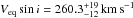 ,
where these uncertainties were computed by properly adding the individual uncertainties
estimated on i and Veq (cf. Table 6 and Fig. 8). This estimated
Veqsini lies between
the lower and intermediate values found in the literature, as mentioned above, and it is
compatible with them within 2σ to 3σ, i.e., ≃30−40 km s-1.
,
where these uncertainties were computed by properly adding the individual uncertainties
estimated on i and Veq (cf. Table 6 and Fig. 8). This estimated
Veqsini lies between
the lower and intermediate values found in the literature, as mentioned above, and it is
compatible with them within 2σ to 3σ, i.e., ≃30−40 km s-1.
Some clues for explaining the discrepancies in the measured Veqsini may be given by the fact that different methods for estimating this quantity can lead to different results depending on their sensitivity to the nonuniform photospheric intensity distribution caused by the gravity darkening. For example, it is known that because of gravity darkening, the Veqsini obtained from visible/IR spectroscopy are generally underestimated in fast-rotating stars (Townsend et al. 2004; Frémat et al. 2005). Moreover, the actual Veqsini of Achernar seems to significantly vary in time, as recently shown by Rivinius et al. (2013), who reported Veqsini variations with amplitudes ≲35 km s-1 that are correlated to the B⇆Be phase transitions. Interestingly, this amplitude of Veqsini variations is on the same order of the differences between the Veqsini values measured in this work and those reported by several other authors, as discussed above.
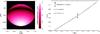 |
Fig. 12 Left: effective temperature map of Achernar corresponding to the
best-fit of the CHARRON RVZ model to the VLTI/PIONIER H band observations
(model parameters in Table 6). The spatial
coordinates are normalized to the measured equatorial radius Req = 9.16
R⊙. The polar and equatorial
effective temperatures of Achernar are Tp = 17 124 K (white) and
Teq = 12
673 K (black). Right: log Teff
as a function of log geff of Achernar for the ELR
model (solid line from Espinosa Lara &
Rieutord 2011). The calculations were performed considering a Roche model
with the same stellar parameters as in Table 6, except for the gravity darkening, which is directly obtained from the
ELR model. The dashed straight line shows the log Teff
versus log geff corresponding to the
best-fit RVZ model with the measured gravity-darkening coefficient β (
= |

Finally, Goss et al. (2011) identified a low-amplitude frequency of 0.68037 ± 0.00003 d-1 from time-series analysis of photometric light-curves of Achernar. We note that this frequency is relatively close (but still ~2.5σ above) to the rotation frequency νrot = 0.644 ± 0.015 d-1 derived in the present work (uncertainty estimated by properly adding quadratically the relative maximum individual uncertainties on Req and Veq). Whether or not the measured frequency is related to the rotation of Achernar remains to be further investigated.
5.4. Gravity darkening
The gravity-darkening parameter β determined in this work is significantly lower than the von Zeipel law (β = 0.25), a result in agreement with β values derived from recent interferometric observations of fast-rotating stars (see for example the recent review from van Belle 2012, and references therein).
These low β
(<0.25) were explained theoretically by Espinosa Lara & Rieutord (2011), who derived an
alternative gravity-darkening law (ELR model hereafter) by relaxing the assumption of
barotropicity that leads to the von Zeipel law. The ELR model includes a divergence-free
flux vector and the ratio  is allowed to vary
with latitude, leading to an analytical relation between Teff and
geff without the need of assuming a
constant β
parameter as in Eq. (3). Let us compare in
more detail the gravity darkening derived from the best-fit of the CHARRON RVZ model with
the prediction from the ELR model. Both models adopt the Roche approximation so that they
consider an identical photospheric shape R(θ). Based on the best-fit
parameters in Table 6, Fig. 12 compares the log Teff versus log geff
relations for the two gravity darkening models. The Teff map of the
RVZ model is also illustrated in Fig. 12. As shown
in the figure, the two models agree within the parameter uncertainties, but the present
observation errors do not yet allow us to probe the small differences in Teff(θ) predicted by the
models.
is allowed to vary
with latitude, leading to an analytical relation between Teff and
geff without the need of assuming a
constant β
parameter as in Eq. (3). Let us compare in
more detail the gravity darkening derived from the best-fit of the CHARRON RVZ model with
the prediction from the ELR model. Both models adopt the Roche approximation so that they
consider an identical photospheric shape R(θ). Based on the best-fit
parameters in Table 6, Fig. 12 compares the log Teff versus log geff
relations for the two gravity darkening models. The Teff map of the
RVZ model is also illustrated in Fig. 12. As shown
in the figure, the two models agree within the parameter uncertainties, but the present
observation errors do not yet allow us to probe the small differences in Teff(θ) predicted by the
models.
Although the detailed Teff(θ) cannot be investigated, it is clear that the ELR model reproduces an average Teff(θ) dependence that is totally compatible with measurements from the RVZ model, but without the need of using a β parameter. Indeed, by estimating an equivalent β value (e.g., from log (Teq/Tp)/log (geq/gp)), Espinosa Lara & Rieutord (2011, in their Fig. 4) showed a good agreement between their predictions and the β coefficients measured on four fast rotators as a function of flattening ϵ (≡1 − Rp/Req).
In Fig. 13 we extend this comparison by adding α Lyr (Vega; Monnier et al. 2012) and Achernar (α Eri; present work). These two new stars provide a crucial test for the ELR model since they have, respectively, the lowest and highest flattening in the sample. Figure 13 thus compares β and ϵ from the ELR model with values measured on six fast rotators (listed from hotter to colder spectral types): α Eri (Achernar, B3-6Vpe; this work), α Leo (Regulus, B8IVn; Che et al. 2011), α Lyr (Vega, A0V; Monnier et al. 2012), α Aql (Altair, A7IV-V; Monnier et al. 2007), α Cep (Alderamin, A7IV; Zhao et al. 2009), β Cas (Caph, F2IV; Che et al. 2011).
Five out of the six stars agree relatively well with the ELR model (in particular Altair and Achernar), considering the observational uncertainties. The only exception is β Cas, and a more detailed study would be required do decide if the discrepancy is due to a bias in the measured flattening related to its low inclination (as discussed by Espinosa Lara & Rieutord 2011) and/or maybe related to the fact that this is star is the coldest one in the sample. This agreement between observational and theoretical results is therefore a promising perspective for a more profound understanding of the gravity-darkening effect in rotating stars.
Based on the curve β versus flattening ϵ given in Fig. 13 and derived from the ELR model, we can deduce a
linear relation that roughly follows this curve: 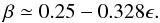 (6)This linear
approximation reproduces the curve in Fig. 13 within
1% (3%) for ϵ ≲ 0.27 (0.30). We recall,
however, that the use of a β parameter is neither required nor compatible with
the ELR model, which does not describe the gravity darkening by a power law as in Eq.
(3).
(6)This linear
approximation reproduces the curve in Fig. 13 within
1% (3%) for ϵ ≲ 0.27 (0.30). We recall,
however, that the use of a β parameter is neither required nor compatible with
the ELR model, which does not describe the gravity darkening by a power law as in Eq.
(3).
5.5. Comparison with the VLTI/AMBER differential phases
We now compare the best-fit CHARRON model determined from the PIONIER data (Table 6) with the AMBER differential phases, described in
Sect. 2.2 and by Domiciano de Souza et al. (2012a). The differential phases computed directly
from the PIONIER best-fit model already well reproduce the AMBER observations, resulting
in  (DOF = 3808). This
χr is only slightly higher than the 1.2
value found by Domiciano de Souza et al. (2012a)
from the same model, but with a somewhat different set of parameters. Indeed, for all
AMBER baselines and wavelengths considered, the absolute differences between both sets of
modeled differential phases are smaller than 0.5°, which is lower than the typical uncertainties in the
differential phases for these AMBER observations (median value of 0.6°).
(DOF = 3808). This
χr is only slightly higher than the 1.2
value found by Domiciano de Souza et al. (2012a)
from the same model, but with a somewhat different set of parameters. Indeed, for all
AMBER baselines and wavelengths considered, the absolute differences between both sets of
modeled differential phases are smaller than 0.5°, which is lower than the typical uncertainties in the
differential phases for these AMBER observations (median value of 0.6°).
 |
Fig. 13 Gravity-darkening coefficient β estimated from the ELR model (Espinosa Lara & Rieutord 2011) as a function of the rotation flattening ϵ compared with values measured from interferometric observations of six rapidly rotating stars (references in Sect. 5.4), Achernar (α Eri) being the flattest one. The estimate of β is obtained from a fit to the log Teff versus log geff curves directly predicted by the ELR model, such as in Fig. 12 (right). The ELR model predictions and interferometric measurements have a good general agreement (see Sect. 5.4 for a more detailed discussion). |
Conversely, the photospheric model parameters derived from the AMBER differential phases
(Domiciano de Souza et al. 2012a) are far from
reproducing the PIONIER observations, resulting in a 10 times higher
 (=19.2).
Moreover, compared to the best-fit model determined in this work, the model from Domiciano de Souza et al. (2012a) presents a worse
agreement with the photometric observations as shown in Table 7 (brighter star in particular because of the higher β and size). Thus, the
CHARRON RVZ photospheric model with parameters as in Table 6 provides the best general agreement with the whole set of polarimetric,
spectroscopic, photometric, and interferometric (PIONIER and AMBER) observations of
Achernar considered in this work.
(=19.2).
Moreover, compared to the best-fit model determined in this work, the model from Domiciano de Souza et al. (2012a) presents a worse
agreement with the photometric observations as shown in Table 7 (brighter star in particular because of the higher β and size). Thus, the
CHARRON RVZ photospheric model with parameters as in Table 6 provides the best general agreement with the whole set of polarimetric,
spectroscopic, photometric, and interferometric (PIONIER and AMBER) observations of
Achernar considered in this work.
6. Beyond the photospheric model ?
We have shown in Sect. 3 that the interferometric data analyzed in this work are not influenced by a strong circumstellar disk or by the known binary companion. This conclusion agrees with the good quality of the fit obtained by adopting a single photospheric fast rotator RVZ model in Sect. 4. In spite of this satisfactory result, and relying on the relatively high-precision PIONIER data, we take the analysis a step farther to search for possible more subtle components in the close environment of Achernar and/or indications of small deviations from the adopted fast-rotator RVZ model. To this aim, two complementary approaches were adopted: (1) model-fitting of the RVZ model plus an additional analytical component; and (2) image reconstruction.
6.1. Photospheric physical model plus analytical component
We used the emcee code to fit a model consisting of the photospheric best-fit RVZ model determined in Sect. 4 plus an analytical 2D Gaussian ellipse. The free parameters of the 2D Gaussian ellipse and their initial range of values (initial uniform distribution of values) are
-
major axis FWHM aGE: 0.5 mas to 20 mas
-
minor-to-major-axis ratio rGE: 0.1 to 1
-
position angle of the major axis PAGE: 0° to 180°
-
flux ratio (relative to the stellar total flux) FGE: 0% to 10%
-
horizontal (equatorial direction) shift relative to the center of the star xGE: − 15 mas to 15 mas
-
vertical (polar direction) shift relative to the center of the star yGE: − 15 mas to 15 mas.
This approach is similar to, but more general than, the one adopted by Kervella & Domiciano de Souza (2006) since it allows to simultaneously test different faint circumstellar structures such as a faint companion or a weak polar wind or equatorial disk.
As before, the emcee algorithm explored the entire parameter space (within the above
defined boundaries) using 800 walkers in a 200 steps burn-in phase and 150 steps in the
final phase. Since the RVZ model already provides a good fit to the data, the parameters
of the additional 2D Gaussian ellipse are not expected to be strongly constrained, leading
to  ,
which is only slightly lower than the value obtained for the RVZ model alone. Two
parameters of the 2D Gaussian ellipse were nevertheless relatively well constrained:
aGE = 5.2 ±
2.4 mas and FGE = 0.7% ± 0.1%. The fit also shows
that the position of this possible additional component is roughly centered on the star,
with a shift uncertainty smaller than ~5 mas for both directions (xGE and yGE). The
remaining parameters are poorly constrained by the data.
,
which is only slightly lower than the value obtained for the RVZ model alone. Two
parameters of the 2D Gaussian ellipse were nevertheless relatively well constrained:
aGE = 5.2 ±
2.4 mas and FGE = 0.7% ± 0.1%. The fit also shows
that the position of this possible additional component is roughly centered on the star,
with a shift uncertainty smaller than ~5 mas for both directions (xGE and yGE). The
remaining parameters are poorly constrained by the data.
6.2. Image reconstruction
As a model-independent study of the PIONIER data we also performed an image
reconstruction of Achernar using the MIRA4 software
(Thiébaut 2008). MIRA is based on an iterative
process, aimed at finding the image that minimizes a joint criterion under constraints of
positivity and normalization,  (7)where x are the set of image
pixels, fdata(x) is the penalty
function of the measurements, fprior(x) is a term
that enforces additional a priori constraints, and μ (≥0) is the hyperparameter, i.e., the weight
of the priors.
(7)where x are the set of image
pixels, fdata(x) is the penalty
function of the measurements, fprior(x) is a term
that enforces additional a priori constraints, and μ (≥0) is the hyperparameter, i.e., the weight
of the priors.
The hyperparameter has to be chosen as large as possible to maximize the weight of the constraints arising from physical modeling and to ensure the convergence of the reconstruction at a minimal value of the penalty χ2. As we have satisfying a model of the target, we used an elliptical Lorentzian a priori (fprior(x)) with (1) the same minor-axis position angle as Achernar, 216.9° (≡36.9° for a centrallysymmetrical ellipse); (2) a major-to-minor axis ratio of 1.3 corresponding to the apparent flattening; and (3) a FWHM = 3.2 mas in the major-axis direction, corresponding to a size slightly bigger than Achernar’s angular diameter, to avoid missing possible structures close to the photosphere.
To determine the best value of the hyperparameter, we performed several (~103) independent reconstructions with 200 iterations and random μ values ranging from
1 to 109. In Fig. 14 (available electronically), we show the distribution of
χ2 for converged reconstructions as a
function of μ
for each reconstruction. This procedure revealed that there is a plateau of minimum
χ2(
=1.4),
reached for values of μ lower than  .
.
After determining the parameters of the reconstruction, we followed the procedure
described by Millour et al. (2012) to create the
reconstructed image of Achernar as the weighted average of several hundred converged
reconstructed images,  (8)where each image
i was
centered on its photocenter position
(8)where each image
i was
centered on its photocenter position  before summation. The weight of each reconstruction is
 , with a limit
penalty value of
, with a limit
penalty value of  to
reject low-quality reconstructed images.
to
reject low-quality reconstructed images.
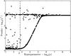 |
Fig. 14 Penalty factor χ2 as a function of the
hyperparameter μ for a set of reconstructed MIRA images
(log scales). Based
on this curve, the value |

Figure 15 shows the reconstructed image of Achernar, both given by MIRA with a 0.07 mas resolution pixel (over-resolved image) and convolved by a Gaussian beam of FWHM = 1.6 mas (diffraction limit of the PIONIER observations). Although this diffraction limit does not provide a highly resolved image of the photosphere, it is enough to investigate the close circumstellar environment. Indeed, the reconstructed MIRA image clearly shows the presence of a compact object (stellar photosphere) without any signature of extended circumstellar component. This is more clearly seen in the right panel of Fig. 15, which shows the subtraction of the MIRA and best-fit CHARRON images, convolved by the 1.6 mas Gaussian beam. The difference between these images is at most 1.5% in modulus (relative to the total flux of the MIRA image) and below ~0.5% almost everywhere.
Both the results from the image reconstruction and from the fit of the RVZ model plus an analytical 2D Gaussian ellipse presented in this section show that no additional component is present in the PIONIER data within ~± 1% level of intensity. This agrees well with the conclusions based on polarimetric and spectroscopic data and modeling shown in Sect. 3.
7. Conclusions
Based on ESO-VLTI interferometric observations of Achernar obtained in a normal B star phase, we derived its photospheric parameters by fitting our physical model CHARRON using a MCMC method. A best-fit photospheric model was derived from squared visibilities and phase closures recorded with the PIONIER beam combiner in the H band. This model agrees well with AMBER HR differential phase observations around the Brγ line.
The interferometric observations were complemented by spectroscopic, polarimetric, and photometric data to investigate the status of the circumstellar environment of Achernar during the VLTI observing runs, to cross-check our model-fitting results, and to set constraints on the model parameter space (photosphere and possible residual disk). In particular, polarimetry was crucial to constrain the disk density, imposing quite well-defined upper limits.
We note that our photospheric model of Achernar agrees with many observations from distinct techniques: PIONIER V2 and CP, AMBER differential phases, V- and B-band polarimetry, Hα and Hβ line profiles, and UBJHK photometry. Moreover, our results are compatible with the theoretical model of gravity darkening proposed by Espinosa Lara & Rieutord (2011, ELR model), which we also showed to be consistent with previously published results from different fast rotators over a wide range of rotational flattening (Achernar being the flattest one in the sample). Observational validation of gravity-darkening models such as the ELR model is an important step in the understanding of rapidly rotating stars since it has the great advantage of reducing the number of free parameters (β coefficient is not needed anymore). Indeed, by relying on a few input parameters and hypotheses, the ELR model reproduces five out of the six measured gravity-darkening β coefficients, which is motivating and promising for a more profound understanding of this important effect in stellar physics.
Taking advantage of the good quality and uv coverage of the PIONIER observations, we also pushed the analysis a little farther and performed an interferometric image reconstruction that did not reveal any signatures of additional circumstellar components and/or deviations from the photospheric Roche-von Zeipel (RVZ) model within a ~± 1% level of intensity. This result also agrees with a fit of an addition analytical component to the RVZ model. Although the spatial resolution of the image is rather low (spatial frequencies restricted to the first visibility lobe), this is, to our knowledge, the first reconstructed image of the photosphere of a Be star.
 |
Fig. 15 Left: image reconstruction of Achernar obtained by applying the MIRA software to the H band VLTI/PIONIER observations. Middle: convolution of this reconstructed MIRA image convolved by a Gaussian beam of FWHM = 1.6 mas (=0.61λ/Bmax) corresponding to the diffraction limit of the PIONIER observations. Right: Reconstructed MIRA image minus the best-fit CHARRON image (Fig. 11 convolved by the Gaussian diffraction limit beam to mach the resolution of reconstructed image). The difference between the images is very small, <1.5% in modulus, relative to the total MIRA image flux), indicating that essentially only the photosphere of Achernar contributes to the PIONIER data, without any additional circumstellar component. The dotted ellipse approximately represents the border of the apparent photosphere of Achernar given by the best-fit CHARRON RVZ model. |
The results of this work thus provide the first determination of the pure photospheric parameters of a Be star in a normal B phase. The measured photospheric parameters are Req, Veq, i, β, and PArot. Concerning Achernar specifically, these parameters can be used as a reference input photospheric model for future studies based on modeling that includes circumstellar disk and photosphere.
Observatório Pico dos Dias/Laboratório Nacional de Astrofísica.
Multi-aperture image reconstruction algorithm.
Available at http://cdsweb.u-strasbg.fr/
Available at http://www.jmmc.fr/oifitsexplorer
Available at http://www.jmmc.fr/searchcal
Acknowledgments
PIONIER is funded by the Université Joseph Fourier (UJF), the Institut de Planétologie et d’Astrophysique de Grenoble (IPAG), the Agence Nationale pour la Recherche (ANR-06-BLAN-0421 and ANR-10-BLAN-0505), and the Institut National des Science de l’Univers (INSU PNP and PNPS). The integrated optics beam combiner is the result of a collaboration between IPAG and CEA-LETI based on CNES R&T funding. This research has made use of the SIMBAD database, operated at the CDS, Strasbourg, France, of NASA Astrophysics Data System Abstract Service5. We also have used the Jean-Marie Mariotti Center (JMMC) services OIFits Explorer 6, and SearchCal 7. This work has made use of the computing facilities (1) of the Mésocentre SIGAMM (hosted by Observatoire de la Côte d’Azur, France), and (2) of the Laboratory of Astroinformatics (IAG/USP and NAT/Unicsul, Brazil), whose purchase was made possible by the Brazilian agency FAPESP (grant 2009/54006-4) and the INCT-A. We thank the CNRS-PICS (France) program 2010-2012 for supporting our Brazilian-French collaboration and the present work. We acknowledge D. Mary and D. Foreman-Mackey for their enlightening suggestions on MCMC methods and on the emcee code. We also thank E. Alecian and T. Rivinius for providing the reduced HARPS and FEROS visible spectra of Achernar.
References
- Absil, O., Mennesson, B., Le Bouquin, J.-B., et al. 2009, ApJ, 704, 150 [NASA ADS] [CrossRef] [Google Scholar]
- Bonneau, D., Clausse, J.-M., Delfosse, X., et al. 2006, A&A, 456, 789 [NASA ADS] [CrossRef] [EDP Sciences] [Google Scholar]
- Bordé, P., Coudé du Foresto, V., Chagnon, G., & Perrin, G. 2002, A&A, 393, 183 [NASA ADS] [CrossRef] [EDP Sciences] [Google Scholar]
- Carciofi, A. C., & Bjorkman, J. E. 2006, ApJ, 639, 1081 [NASA ADS] [CrossRef] [Google Scholar]
- Carciofi, A. C., Magalhães, A. M., Leister, N. V., Bjorkman, J. E., & Levenhagen, R. S. 2007, ApJ, 671, L49 [NASA ADS] [CrossRef] [Google Scholar]
- Carciofi, A. C., Domiciano de Souza, A., Magalhães, A. M., Bjorkman, J. E., & Vakili, F. 2008, ApJ, 676, L41 [NASA ADS] [CrossRef] [Google Scholar]
- Chauville, J., Zorec, J., Ballereau, D., et al. 2001, A&A, 378, 861 [NASA ADS] [CrossRef] [EDP Sciences] [Google Scholar]
- Che, X., Monnier, J. D., Zhao, M., et al. 2011, ApJ, 732, 68 [NASA ADS] [CrossRef] [Google Scholar]
- Code, A. D., Bless, R. C., Davis, J., & Brown, R. H. 1976, ApJ, 203, 417 [NASA ADS] [CrossRef] [Google Scholar]
- Cohen, M., Walker, R. G., Carter, B., et al. 1999, AJ, 117, 1864 [NASA ADS] [CrossRef] [Google Scholar]
- Cutri, R. M., Skrutskie, M. F., van Dyk, S., et al. 2003, VizieR Online Data Catalog: II/246 [Google Scholar]
- Domiciano de Souza, A., Vakili, F., Jankov, S., Janot-Pacheco, E., & Abe, L. 2002, A&A, 393, 345 [NASA ADS] [CrossRef] [EDP Sciences] [Google Scholar]
- Domiciano de Souza, A., Kervella, P., Jankov, S., et al. 2003, A&A, 407, L47 [NASA ADS] [CrossRef] [EDP Sciences] [Google Scholar]
- Domiciano de Souza, A., Hadjara, M., Vakili, F., et al. 2012a, A&A, 545, A130 [NASA ADS] [CrossRef] [EDP Sciences] [Google Scholar]
- Domiciano de Souza, A., Zorec, J., & Vakili, F. 2012b, in SF2A-2012: Proc. Annual meeting of the French Society of Astronomy and Astrophysics, eds. S. Boissier, P. de Laverny, N. Nardetto, et al. 321 [Google Scholar]
- Espinosa Lara, F., & Rieutord, M. 2011, A&A, 533, A43 [NASA ADS] [CrossRef] [EDP Sciences] [Google Scholar]
- Foreman-Mackey, D., Hogg, D. W., Lang, D., & Goodman, J. 2013, PASP, 125, 306 [CrossRef] [Google Scholar]
- Frémat, Y., Zorec, J., Hubert, A., & Floquet, M. 2005, A&A, 440, 305 [NASA ADS] [CrossRef] [EDP Sciences] [Google Scholar]
- Goodman, J., & Weare, J. 2010, Commun. Appl. Math. Comput. Sci., 5, 65 [Google Scholar]
- Goss, K. J. F., Karoff, C., Chaplin, W. J., Elsworth, Y., & Stevens, I. R. 2011, MNRAS, 411, 162 [NASA ADS] [CrossRef] [Google Scholar]
- Haguenauer, P., Alonso, J., Bourget, P., et al. 2010, in SPIE Conf. Ser., 7734, 04 [Google Scholar]
- Hanbury Brown, R., Davis, J., & Allen, L. R. 1974, MNRAS, 167, 121 [NASA ADS] [CrossRef] [Google Scholar]
- Harmanec, P. 1988, Bull. Astron. Inst. Czechosl., 39, 329 [Google Scholar]
- Haubois, X., Carciofi, A. C., Rivinius, T., Okazaki, A. T., & Bjorkman, J. E. 2012, ApJ, 756, 156 [NASA ADS] [CrossRef] [Google Scholar]
- Hog, E., Fabricius, C., Makarov, V. V., et al. 2000, VizieR Online Data Catalog: I/259 [Google Scholar]
- Hubeny, I., & Lanz, T. 2011, Synspec: General Spectrum Synthesis Program, astrophysics Source Code Library [Google Scholar]
- Hutchings, J. B., & Stoeckley, T. R. 1977, PASP, 89, 19 [NASA ADS] [CrossRef] [Google Scholar]
- Jackson, S., MacGregor, K. B., & Skumanich, A. 2004, ApJ, 606, 1196 [NASA ADS] [CrossRef] [Google Scholar]
- Jaschek, M., & Egret, D. 1982, in Be Stars, eds. M. Jaschek, & H.-G. Groth, IAU Symp., 98, 261 [Google Scholar]
- Jerzykiewicz, M., & Molenda-Zakowicz, J. 2000, Acta Astron., 50, 369 [NASA ADS] [Google Scholar]
- Johnson, H. L., Mitchell, R. I., Iriarte, B., & Wisniewski, W. Z. 1966, Communications of the Lunar and Planetary Laboratory, 4, 99 [Google Scholar]
- Kervella, P., & Domiciano de Souza, A. 2006, A&A, 453, 1059 [NASA ADS] [CrossRef] [EDP Sciences] [Google Scholar]
- Kervella, P., & Domiciano de Souza, A. 2007, A&A, 474, L49 [NASA ADS] [CrossRef] [EDP Sciences] [Google Scholar]
- Kervella, P., Thévenin, F., Morel, P., Bordé, P., & Di Folco, E. 2003, A&A, 408, 681 [NASA ADS] [CrossRef] [EDP Sciences] [Google Scholar]
- Kervella, P., Domiciano de Souza, A., & Bendjoya, P. 2008, A&A, 484, L13 [NASA ADS] [CrossRef] [EDP Sciences] [Google Scholar]
- Kurucz, R. L. 1979, ApJS, 40, 1 [NASA ADS] [CrossRef] [Google Scholar]
- Lafrasse, S., Mella, G., Bonneau, D., et al. 2010, in SPIE Conf. Ser., 7734 [Google Scholar]
- LeBouquin, J.-B., Berger, J.-P., Lazareff, B., et al. 2011, A&A, 535, A67 [NASA ADS] [CrossRef] [EDP Sciences] [Google Scholar]
- Maeder, A., & Meynet, G. 2000, ARA&A, 38, 143 [NASA ADS] [CrossRef] [Google Scholar]
- Magalhães, A. M., Benedetti, E., & Roland, E. H. 1984, PASP, 96, 383 [NASA ADS] [CrossRef] [Google Scholar]
- Magalhães, A. M., Rodrigues, C. V., Meade, M., et al. 1996, in Polarimetry of the Interstellar Medium, eds. W. G. Roberge & D. C. B. Whittet, ASP Conf. Ser., 97, 202 [Google Scholar]
- Millour, F. A., Vannier, M., & Meilland, A. 2012, in SPIE Conf. Ser., 8445 [Google Scholar]
- Monnier, J. D., Zhao, M., Pedretti, E., et al. 2007, Science, 317, 342 [NASA ADS] [CrossRef] [PubMed] [Google Scholar]
- Monnier, J. D., Che, X., Zhao, M., et al. 2012, ApJ, 761, L3 [NASA ADS] [CrossRef] [Google Scholar]
- Nazé, Y. 2009, A&A, 506, 1055 [NASA ADS] [CrossRef] [EDP Sciences] [Google Scholar]
- Rivinius, T., Baade, D., Townsend, R. H. D., Carciofi, A. C., & Štefl, S. 2013, A&A, 559, L4 [NASA ADS] [CrossRef] [EDP Sciences] [Google Scholar]
- Skrutskie, M. F., Cutri, R. M., Stiening, R., et al. 2006, AJ, 131, 1163 [NASA ADS] [CrossRef] [Google Scholar]
- Slettebak, A. 1982, ApJS, 50, 55 [NASA ADS] [CrossRef] [Google Scholar]
- Thiébaut, E. 2008, in SPIE Conf. Ser., 7013 [Google Scholar]
- Townsend, R. H. D., Owocki, S. P., & Howarth, I. D. 2004, MNRAS, 350, 189 [Google Scholar]
- van Belle, G. T. 2012, A&ARv, 20, 51 [NASA ADS] [CrossRef] [Google Scholar]
- van Leeuwen, F. 2007, A&A, 474, 653 [NASA ADS] [CrossRef] [EDP Sciences] [Google Scholar]
- Vinicius, M. M. F., Zorec, J., Leister, N. V., & Levenhagen, R. S. 2006, A&A, 446, 643 [NASA ADS] [CrossRef] [EDP Sciences] [Google Scholar]
- von Zeipel, H. 1924, MNRAS, 84, 665 [NASA ADS] [CrossRef] [Google Scholar]
- Zacharias, N., Monet, D. G., Levine, S. E., et al. 2005, VizieR Online Data Catalog: I/297 [Google Scholar]
- Zhao, M., Monnier, J. D., Pedretti, E., et al. 2009, ApJ, 701, 209 [NASA ADS] [CrossRef] [Google Scholar]
All Tables
Summary of broadband polarization data that are contemporaneous to the VLTI observations.
Summary of spectroscopic data of Achernar that are contemporaneous to the VLTI observations.
Physical parameters of Achernar derived from the fit of the RVZ model (CHARRON code) to VLTI/PIONIER H band data using the MCMC method (emcee code).
All Figures
|
Fig. 1 uv coverage of VLTI/PIONIER observations of Achernar. The AT baselines used are identified with different colors. Image adapted from the OIFITSExplorer/JMMC tool. |
| In the text | |
|
Fig. 2 Polarimetric observations at the epochs of ESO-VLTI AMBER and PIONIER data of Achernar analyzed in this work (vertical hatched bars). All the measurements are compatible with null/negligible polarization. The horizontal gray bars indicate the weighted average of the polarization: 0.019 ± 0.012%. Vertical lines correspond to epochs of Hα (dotted) and Hβ (dot-dashed) data observations with colors corresponding to the spectra shown in Fig. 3. The spectroscopic and polarimetric data are thus contemporaneous and embrace the interferometric observations in time. |
| In the text | |
|
Fig. 3 Top: Hα (left) and Hβ (right) line profiles of Achernar at the epoch of interferometric observations. Bottom: difference in flux of the line profiles with respect to the reference FEROS spectrum from 2000 Jan. 11. This spectrum can be considered as a good approximation to the pure photospheric profile of Achernar (Rivinius et al. 2013). Whenever possible (enough spectral resolution) the telluric lines seen in some spectra have been removed before computing the differences. The horizontal shaded (gray) areas indicate the typical error on the difference profiles and also set a limit to them. |
| In the text | |
|
Fig. 4 Polarization in the B band (left) and standard deviation of difference Hα profile (right) as a function of disk-base density ρ0 for the residual disk models from Table 5 (model 1: full line; model 2: dashed line). The standard deviation is the root mean square of the disk model spectrum minus the pure photospheric profile. The horizontal dot-dashed lines represent the observational limits of average polarization and difference profile determined from observations performed at the epoch of interferometric observations, as explained in Sect. 3. While the measured Hα difference profile level does not impose a limit to ρ0, the measured average polarization sets a strict upper limit to this quantity: ρ0< 0.52 × 10⁻¹² g cm-3 for the thin-disk model and ρ0< 0.65 × 10⁻¹² g cm-3 for the thick-disk model. |
| In the text | |
|
Fig. 5 Top: Hα line profile for the pure photospheric model (black solid line) and with a residual disk (VDD model) as defined in Table 5 and computed for the upper limit values of ρ0 (cf. Fig. 4): 0.52 × 10⁻¹² g cm-3 (thin disk; blue solid line) and 0.65 × 10⁻¹² g cm-3 (thick disk; blue dashed line). Bottom: the difference between the disk models relative to the photospheric model. The observational limit set to the difference profiles defined in Sect. 3 is indicated by the shaded (gray) region. |
| In the text | |
|
Fig. 6 Interferometric observables, squared visibilities V2 in the H band (left), and Brγ differential phases (right), computed for the pure photospheric model (black solid line) and for the two residual-disk models as defined in Table 5 at the upper limit values of ρ0 (cf. Fig. 4): 0.52 × 10⁻¹² g cm-3 (thin disk; blue solid line) and 0.65 × 10⁻¹² g cm-3 (thick disk; blue dashed line). The baseline position angle PA was chosen to lie along the stellar equator (cf. Sect. 4.2), so that the effects of the residual disk are maximized on these comparisons. The baseline length for the differential phase calculations roughly corresponds to half of the maximum available length. Bottom: the difference between the interferometric observables from the disk models relative to the photospheric model. The shaded areas correspond to the typical observational errors from our PIONIER and AMBER observations. These difference plots show that the disk contribution to the interferometric observables is only a small fraction of the observation errors even at the upper limit ρ0, discarding any detectable influence of a circumstellar disk on the present interferometric observations of Achernar. |
| In the text | |
|
Fig. 7 Convergence of equatorial radius Req during the burn-in phase of the MCMC fit of the CHARRON RVZ model to the VLTI/PIONIER data using the emcee code (800 walkers and 200 iteration steps). |
| In the text | |
|
Fig. 8 Histogram distributions and two-by-two correlations for the free parameters (Req, Veq, i, β, and PArot) of the best-fit CHARRON RVZ model determined with the emcee code (800 walkers). The mean values and associated uncertainties obtained from these histograms are given in Table 6. The parameters do not show strong correlations in the region defined by the uncertainty around the mean values. The stronger correlation is shown by Veq and i, which roughly follow a curve of constant Veqsini (=260.3 km s-1), represented by the solid lines, with the circles indicating the mean values in the histograms. The rectangles cover the corresponding uncertainty ranges on Veq and i. |
| In the text | |
|
Fig. 9 Top: squared visibilities V2 observed on Achernar (filled circles and error bars) and computed (opened squares) from the best-fit CHARRON model (Table 6) as a function of spatial frequency (left column) and baseline PA (right column). Bottom: V2 residuals from observations relative to the best-fit model in units of corresponding uncertainties. Vertical solid lines indicate the position angles of the visible (216.9° ≡ −143.1°) and hidden (16.9° = 216.9°−180°) stellar poles. The horizontal dotted lines delimit the ± 3σ region around zero (dashed line). |
| In the text | |
|
Fig. 10 Top: closure phases (CP) observed on Achernar and computed from
the best-fit CHARRON model (Table 6) as a
function of the spatial frequency (for the longest projected baseline
|
| In the text | |
|
Fig. 11 Intensity map of Achernar corresponding to the best-fit of the CHARRON RVZ model to the VLTI/PIONIER H band observations. The spatial coordinates indicated in angular milliarcseconds (mas) units and also normalized to the equatorial radius Req = 9.16 R⊙. The complete list of the measured stellar parameters is given in Table 6. |
| In the text | |
|
Fig. 12 Left: effective temperature map of Achernar corresponding to the
best-fit of the CHARRON RVZ model to the VLTI/PIONIER H band observations
(model parameters in Table 6). The spatial
coordinates are normalized to the measured equatorial radius Req = 9.16
R⊙. The polar and equatorial
effective temperatures of Achernar are Tp = 17 124 K (white) and
Teq = 12
673 K (black). Right: log Teff
as a function of log geff of Achernar for the ELR
model (solid line from Espinosa Lara &
Rieutord 2011). The calculations were performed considering a Roche model
with the same stellar parameters as in Table 6, except for the gravity darkening, which is directly obtained from the
ELR model. The dashed straight line shows the log Teff
versus log geff corresponding to the
best-fit RVZ model with the measured gravity-darkening coefficient β (
= |
| In the text | |
|
Fig. 13 Gravity-darkening coefficient β estimated from the ELR model (Espinosa Lara & Rieutord 2011) as a function of the rotation flattening ϵ compared with values measured from interferometric observations of six rapidly rotating stars (references in Sect. 5.4), Achernar (α Eri) being the flattest one. The estimate of β is obtained from a fit to the log Teff versus log geff curves directly predicted by the ELR model, such as in Fig. 12 (right). The ELR model predictions and interferometric measurements have a good general agreement (see Sect. 5.4 for a more detailed discussion). |
| In the text | |
|
Fig. 14 Penalty factor χ2 as a function of the
hyperparameter μ for a set of reconstructed MIRA images
(log scales). Based
on this curve, the value |
| In the text | |
|
Fig. 15 Left: image reconstruction of Achernar obtained by applying the MIRA software to the H band VLTI/PIONIER observations. Middle: convolution of this reconstructed MIRA image convolved by a Gaussian beam of FWHM = 1.6 mas (=0.61λ/Bmax) corresponding to the diffraction limit of the PIONIER observations. Right: Reconstructed MIRA image minus the best-fit CHARRON image (Fig. 11 convolved by the Gaussian diffraction limit beam to mach the resolution of reconstructed image). The difference between the images is very small, <1.5% in modulus, relative to the total MIRA image flux), indicating that essentially only the photosphere of Achernar contributes to the PIONIER data, without any additional circumstellar component. The dotted ellipse approximately represents the border of the apparent photosphere of Achernar given by the best-fit CHARRON RVZ model. |
| In the text | |
Current usage metrics show cumulative count of Article Views (full-text article views including HTML views, PDF and ePub downloads, according to the available data) and Abstracts Views on Vision4Press platform.
Data correspond to usage on the plateform after 2015. The current usage metrics is available 48-96 hours after online publication and is updated daily on week days.
Initial download of the metrics may take a while.