| Issue |
A&A
Volume 568, August 2014
|
|
|---|---|---|
| Article Number | A31 | |
| Number of page(s) | 11 | |
| Section | The Sun | |
| DOI | https://doi.org/10.1051/0004-6361/201323352 | |
| Published online | 08 August 2014 | |
Standing sausage modes in coronal loops with plasma flow⋆
Shandong Provincial Key Laboratory of Optical Astronomy and
Solar-Terrestrial Environment, School of Space Science and Physics, Shandong
University at Weihai,
264209
Weihai,
PR China
e-mail:
This email address is being protected from spambots. You need JavaScript enabled to view it.
Received:
29
December
2013
Accepted:
18
June
2014
Abstract
Context. Magnetohydrodynamic waves are important for diagnosing the physical parameters of coronal plasmas. Field-aligned flows appear frequently in coronal loops.
Aims. We examine the effects of transverse density and plasma flow structuring on standing sausage modes trapped in coronal loops, and examine their observational implications in the context of coronal seismology.
Methods. We model coronal loops as straight cold cylinders with plasma flow embedded in a static corona. An eigen-value problem governing propagating sausage waves is formulated and its solutions are employed to construct standing modes. Two transverse profiles are distinguished, and are called profiles E and N. A parameter study is performed on the dependence of the maximum period Pmax and cutoff length-to-radius ratio (L/a)cutoff in the trapped regime on the density parameters (ρ0/ρ∞ and profile steepness p) and the flow parameters (its magnitude U0 and profile steepness u).
Results. For either profile, introducing a flow reduces Pmax obtainable in the trapped regime relative to the static case. The value of Pmax is sensitive to p for profile N, but is insensitive to p for profile E. By far the most important effect a flow introduces is to reduce the capability for loops to trap standing sausage modes: (L/a)cutoff may be substantially reduced in the case with flow relative to the static one. In addition, (L/a)cutoff is smaller for a stronger flow, and for a steeper flow profile when the flow magnitude is fixed.
Conclusions. If the density distribution can be described by profile N, then measuring the sausage mode period can help deduce the density profile steepness. However, this practice is not feasible if profile E more accurately describes the density distribution. Furthermore, even field-aligned flows with magnitudes substantially smaller than the ambient Alfvén speed can make coronal loops considerably less likely to support trapped standing sausage modes.
Key words: magnetohydrodynamics (MHD) / Sun: corona / Sun: magnetic fields / waves
Appendix A is available in electronic form at http://www.aanda.org
© ESO, 2014
1. Introduction
Capitalizing on the abundantly identified magnetohydrodynamic (MHD) waves and oscillations in the solar atmosphere, coronal seismology (Roberts et al.1984; also Zaitsev & Stepanov1975; Uchida1970) proves to be a powerful tool for diagnosing the atmospheric parameters that are difficult to directly yield (for recent reviews, see De Moortel & Nakariakov2012; and also Ballester et al.2007; Nakariakov & Erdélyi2009; Erdélyi & Goossens2011 for three recent topical issues). This rapidly growing branch of solar physics, with its applications now extended beyond the solar corona (e.g., Banerjee et al. 2007), gained its theoretical foundation with a detailed analysis of the modes collectively supported by a straight magnetic cylinder with density higher than in its surroundings (Edwin & Roberts1983; and also Zaitsev & Stepanov1975). The axially symmetric mode, for which the azimuthal wavenumber is zero, is among the infinitely many collective modes. When oscillating in this mode, a coronal loop experiences periodical changes of the loop cross-section in anti-phase with the density variation, with the perturbed fluid velocity primarily transverse (e.g., Pascoe et al. 2007a,b; Gruszecki et al. 2012).
Possibly associated with the quasi-periodic oscillations in lightcurves related to solar flares, sausage modes can play an important role in seismologically diagnosing the physical parameters in the region where flare energy is released (see Nakariakov & Melnikov 2009, for a recent review). Their role in such a context was first postulated by Rosenberg (1970) to account for microwave measurements, but extends also to the interpretation of measurements in hard X-Ray and white light (Zaitsev & Stepanov 1982). A wealth of potential candidates in spatially unresolved radio observations that may be associated with sausage oscillations exists (see Table 1 compiled in Aschwanden et al.2004), which is enriched with spatially resolved instances found with the Nobeyama Radioheliograph (NRH) data (Nakariakov et al.2003, hereafter NMR03; Melnikov et al.2005; Inglis et al.2008). More recently, sausage oscillations were also found by Su et al. (2012) using the imaging data acquired by the Atmospheric Imaging Assembly (AIA, Lemen et al.2012) on board the Solar Dynamics Observatory (SDO, Pesnell et al.2012). They were identified in the observations made with the Rapid Oscillations in the Solar Atmosphere (ROSA) imager as well (Morton et al. 2012).
Among the parameters that sausage mode observations can offer, the magnetic field strength in the flaring region tops the list (Nakariakov et al. 2003), while the density contrast of the flaring loop relative to its ambient corona and the plasma β can be serendipitously found when fast sausage modes occur simultaneously with slow modes (Van Doorsselaere et al. 2011). We note that a forward modeling approach has also been adopted to examine the observability of sausage modes in the optically thin radiation in general (Gruszecki et al. 2012), and in the Extreme Ultraviolet (Antolin & Van Doorsselaere 2013) as well as radio passbands (Reznikova et al. 2014) in particular. It turns out that such factors as viewing angles as well as spectral, temporal, and spatial resolution may all be important as far as the detectability of sausage modes is concerned.
Sausage modes are well known to have two distinct regimes. Those with axial wavenumbers larger than a cutoff kc correspond to the trapped regime with the oscillations confined in the loop. The leaky regime arises when the opposite is true, and the sausage modes are subject to damping by radiating their energy into the surrounding fluid (Zaitsev & Stepanov 1975; Kopylova et al. 2007). However, that a sausage mode is in the leaky regime does not necessarily mean that it is not observationally accessible, provided that the quality factor Q = τ/P is sufficiently high, where τ and P denote the damping time and period, respectively. In the idealized case where the parameters of the loop (denoted by the subscript 0) and its surroundings (subscript ∞) are piece-wise constant, both kc (Edwin & Roberts 1983) and Q (Kopylova et al. 2007) turn out to depend primarily on the density contrast ρ0/ρ∞ in a low beta environment. Regarding standing sausage modes, the wavenumber cutoff kc corresponds to a critical loop length-to-radius ratio (L/a)cutoff, which separates standing modes into trapped and leaky ones. Modes in the former (latter) category correspond to real (complex) solutions to the relevant dispersion relations. When the loop radius a is fixed, P increases with increasing loop length L until L/a reaches the cutoff value. A further increase in L leads the sausage oscillations into the leaky regime, where P turns out to increase with L as well and shows saturation in the thin-tube limit (L/a ≫ 1). This behavior of sausage mode periods was analytically shown by Zaitsev & Stepanov (1975); Vasheghani Farahani et al. (2014), and numerically demonstrated both via analysing the relevant dispersion diagrams (Kopylova et al. 2007) and by solving the problem as an initial-boundary value one (Pascoe et al. 2007a; Inglis et al. 2009; Nakariakov et al. 2012).
Several aspects of the recent study by Nakariakov et al. (2012, hereafter NHM12) are noteworthy. First, regarding a step-function transverse density profile, the maximum period that trapped sausage modes can attain (denoted by Pstep and explicitly given by Eq. (5)) is only marginally smaller than the saturation value attained in the thin-tube limit in the leaky regime (Fig. 3 in NHM12, also Fig. 2 in Vasheghani Farahani et al.2014). Actually, solving Eq. (40) in Vasheghani Farahani et al. (2014) appropriate for the k = 0 limit, we found that the period P is larger than Pstep by less than 11.3% for density ratios higher than 10. Second, the tendency for the sausage mode period to increase with loop length before reaching saturation also holds for the smooth density profiles considered therein, with the saturation period increasing with the profile steepness in a sensitive manner. Consequently, the period measurements of standing oscillations may then have the potential to diagnose how steep the transverse density distribution is, thereby adding yet another important item to the list of the atmospheric parameters that can be seismologically deduced. Another consequence is that, Pstep as obtained in the infinitely steep case would be a good approximate upper limit for the sausage mode periods when ρ0/ρ∞ ≳ 10. Given a typical loop radius a ~ 103 km, and an internal Alfvén speed vA0 ~ 103km s-1, this justifies the notion that standing sausage modes are responsible primarily for second-scale oscillations in flare lightcurves (Aschwanden et al. 2004).
There are two objectives to the present study. First, does the maximum period obtainable in the trapped regime depend on the density profile steepness in a monotonic way for all choices of density profiles? To this end, in addition to the profile chosen in NHM12, we also examine another profile which has been in wide use in the literature. Second, what would be the effects of a field-aligned loop flow on standing sausage modes? This is necessary given that loop flows reaching up to ~100 km s-1 seem ubiquitous in the corona in general (Sect. 4.4 in Aschwanden2004, see also Del Zanna2008 and Tripathi et al.2012 for more recent results with the Hinode EUV Imaging Spectrometer), and have been found in oscillating structures in particular (Ofman & Wang 2008). While previous studies on the flow effects are concerned mainly with kink modes (Gruszecki et al. 2008; Ruderman 2010), the present study is focused on sausage modes. Of particular interest is the behavior of the maximum period Pmax and maximum length-to-radius ratio allowed in the trapped regime.
Before proceeding, a few words on the approach to be used seem necessary. We model coronal loops as a monolithic, straight, axially uniform, magnetic cylinder embedded in an ambient corona, and examine linear, trapped sausage oscillations in the framework of zero-beta, ideal MHD. By seeing loops as being monolithic, we neglect the possible effects of them being multithreaded or involving other forms of structuring. We note that for loops structured as a bundle of concentric shells, the fine structuring effect seems marginal (Pascoe et al. 2007b). The same can be said about the effects both due to the longitudinal variation of the background parameters (Pascoe et al. 2009) and to the finite plasma beta (Inglis et al. 2009). Furthermore, the loop curvature is known to couple the sausage to kink modes (Roberts 2000; Van Doorsselaere et al. 2009); however, its influence on the properties of sausage modes remains to be assessed by a dedicated study. It should also be stressed that only trapped modes are to be examined. While this approach is acceptable to find the dividing line separating the leaky and trapped regimes, it does not allow us to draw a definitive conclusion on whether the sausage periods saturate in the long-wavelength limit for general transverse density profiles in the case with flow. That is why Pmax, the maximum period that trapped sausage modes may attain, is used. Nonetheless, from Fig. 3 in NHM12 (see also Fig. 4 in the present manuscript), it seems reasonable to speculate that a saturation exists and the saturation period is not far from Pmax. With this in mind, we are also interested in knowing whether Pmax can be larger than Pstep for profiles other than those adopted in NHM12. If this is indeed the case, then one expects to broaden the range of periods of the quasi-periodic oscillations for which standing sausage modes may account.
This manuscript is organized as follows. In Sect. 2, we offer a brief derivation of the equations governing propagating sausage waves, and explain the procedure for constructing standing modes. Section 3 presents the numerical results, paying special attention to how a smooth transverse profile together with a loop flow affect the characteristics of the standing modes. Finally, a summary is given in Sect. 4.
2. Problem formulation and construction of standing sausage modes
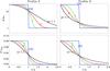 |
Fig. 1 Background density |


The coronal loop is modeled as a straight cylinder with field-aligned flow and enhanced
density embedded in a uniform magnetic field  .
(The barred quantities refer to the equilibrium parameters.) Both the cylinder axis and
lie in the z-direction in a standard cylindrical coordinate system
(r,θ,z). The
equilibrium parameters, namely the flow speed
.
(The barred quantities refer to the equilibrium parameters.) Both the cylinder axis and
lie in the z-direction in a standard cylindrical coordinate system
(r,θ,z). The
equilibrium parameters, namely the flow speed  and background density
  ,
are structured only in the r-direction. We distinguish between two profiles. One
is described by
,
are structured only in the r-direction. We distinguish between two profiles. One
is described by ![Mathematical equation: \begin{eqnarray} && \bar{\rho}(r)=\rho_\infty+(\rho_0-\rho_\infty){\rm sech}^2\left[\left(\displaystyle\frac{r}{a}\right)^p\right]~, \nonumber \\ \label{eq_profileE} && \bar{U}(r) =U_0{\rm sech}^2\left[\left(\displaystyle\frac{r}{a}\right)^u\right] , \end{eqnarray}](/articles/aa/full_html/2014/08/aa23352-13/aa23352-13-eq39.png) (1)which
is a generalized Epstein profile and called profile E for brevity. When p = 1, it yields the familiar
symmetric Epstein profile for the density distribution, which has been extensively employed
in the literature to study standing modes supported by static loops (e.g., Cooper et al. 2003; Pascoe
et al. 2007a; Chen et al. 2013). The profiles
with p>
1 were further explored by Nakariakov
& Roberts (1995) in the context of impulsively excited sausage waves. The
other profile is given by
(1)which
is a generalized Epstein profile and called profile E for brevity. When p = 1, it yields the familiar
symmetric Epstein profile for the density distribution, which has been extensively employed
in the literature to study standing modes supported by static loops (e.g., Cooper et al. 2003; Pascoe
et al. 2007a; Chen et al. 2013). The profiles
with p>
1 were further explored by Nakariakov
& Roberts (1995) in the context of impulsively excited sausage waves. The
other profile is given by ![Mathematical equation: \begin{eqnarray} && \bar{\rho}(r)=\rho_\infty\left\{1-\left(1-\sqrt{\displaystyle \frac{\rho_\infty}{\rho_0}}\right)\exp \left[-\left(\displaystyle\frac{r}{a}\right)^p\right] \right\}^{-2}, \nonumber \\ \label{eq_profileN} && \bar{U}(r)=U_0\exp\left[-\left(\displaystyle\frac{r}{a}\right)^u\right], \end{eqnarray}](/articles/aa/full_html/2014/08/aa23352-13/aa23352-13-eq42.png) (2)and
is called profile N given that it was proposed in NHM12, albeit expressed in terms of the
Alfvén speed profile therein. By defining
(2)and
is called profile N given that it was proposed in NHM12, albeit expressed in terms of the
Alfvén speed profile therein. By defining  ,
one readily recovers Eq. (1) in NHM12. Both density profiles give a distribution smoothly
decreasing from ρ0 at r = 0 to ρ∞ when
r → ∞.
Consequently, the Alfvén speed
,
one readily recovers Eq. (1) in NHM12. Both density profiles give a distribution smoothly
decreasing from ρ0 at r = 0 to ρ∞ when
r → ∞.
Consequently, the Alfvén speed  ,
where μ is the
magnetic permeability of free space, increases smoothly from vA0 at
r = 0 to
vA∞ at large distances. For either profile,
the flow distribution is written following the same spirit as the density distribution. In
fact, the difference between the flow profiles is not significant, both yielding a
distribution that decreases from U0 at r = 0 to zero far from the
cylinder, representing a loop with flow placed in a static ambient corona. In Fig. 1, the two profiles are depicted for a series of
p and
u, with the
combination of [
ρ0/ρ∞,U0
] taken to be [
25,0.08 vA∞ ] for
illustrative purposes. Evidently, for both profiles, the larger the steepness
p or
u, the closer
they are to a step function.
,
where μ is the
magnetic permeability of free space, increases smoothly from vA0 at
r = 0 to
vA∞ at large distances. For either profile,
the flow distribution is written following the same spirit as the density distribution. In
fact, the difference between the flow profiles is not significant, both yielding a
distribution that decreases from U0 at r = 0 to zero far from the
cylinder, representing a loop with flow placed in a static ambient corona. In Fig. 1, the two profiles are depicted for a series of
p and
u, with the
combination of [
ρ0/ρ∞,U0
] taken to be [
25,0.08 vA∞ ] for
illustrative purposes. Evidently, for both profiles, the larger the steepness
p or
u, the closer
they are to a step function.
For future reference, we summarize the relevant information in the zero-beta MHD on sausage
modes supported by static loops where the transverse density distribution is of a
step-function form. The quantities are to be denoted by a superscript “step”. First, the
cutoff wavenumber is given by  (3)where j0,0 =
2.4048 is the first zero of Bessel function J0 (Edwin & Roberts 1983). The corresponding maximum
length-to-radius ratio, only below which the loops can support trapped sausage modes, is
given by
(3)where j0,0 =
2.4048 is the first zero of Bessel function J0 (Edwin & Roberts 1983). The corresponding maximum
length-to-radius ratio, only below which the loops can support trapped sausage modes, is
given by  (4)Letting Pstep denote the
period attained at this L/a, one finds
(4)Letting Pstep denote the
period attained at this L/a, one finds
 (5)which is accurately
approximated by 2.62a/vA0
for high density contrasts.
(5)which is accurately
approximated by 2.62a/vA0
for high density contrasts.
We adopt the ideal, zero-beta, MHD equations to describe axisymmetrical (∂/∂θ ≡
0) sausage waves. We let v and b represent the
magnetic field and velocity perturbations, respectively. The relevant equations are then
 Appropriate
for sausage waves, a perturbation f(r,z;t) may be
Fourier decomposed in z and time t,
Appropriate
for sausage waves, a perturbation f(r,z;t) may be
Fourier decomposed in z and time t, ![Mathematical equation: \begin{eqnarray} f(r,z;t)={\rm Re}\{\tilde{f}(r)\exp[-{\rm i}(\omega t-kz)]\}, \label{Fourier} \end{eqnarray}](/articles/aa/full_html/2014/08/aa23352-13/aa23352-13-eq65.png) (8)where
k is the
axial wavenumber, and ω is the angular frequency. The phase speed is then
vph =
ω/k. Letting
′ = d /
dr, one finds from Eqs.(6) and (7) that
(8)where
k is the
axial wavenumber, and ω is the angular frequency. The phase speed is then
vph =
ω/k. Letting
′ = d /
dr, one finds from Eqs.(6) and (7) that
 \We
note that the z-component of the momentum equation is not relevant,
although
\We
note that the z-component of the momentum equation is not relevant,
although  does not vanish when
  is not zero. With the aid of Eq. (11), one
readily sees that Eq. (10) is equivalent to
is not zero. With the aid of Eq. (11), one
readily sees that Eq. (10) is equivalent to
 , namely
the requirement that ∇·b = 0. Using this relation together
with Eq. (11) to eliminate
, namely
the requirement that ∇·b = 0. Using this relation together
with Eq. (11) to eliminate
 and
and  from Eq. (9), one finds
 ![Mathematical equation: \begin{eqnarray} [\vph-\bar{U}(r)]^2\tilde{b}_r(r)=-\frac{v^2_{\rm A}(r)} {k^2}\left[\frac{\mathrm{d}^2}{\mathrm{d}r^2} +\frac{1}{r}\frac{\mathrm{d}}{\mathrm{d}r} -\left(k^2+\frac{1}{r^2}\right)\right]\tilde{b}_r(r) . \label{eq_eigen_br} \end{eqnarray}](/articles/aa/full_html/2014/08/aa23352-13/aa23352-13-eq77.png) (12)The
boundary conditions required for formulating a standard eigen-value problem for sausage
waves are usually specified in terms of the radial velocity perturbation
.
To be specific, these are
(12)The
boundary conditions required for formulating a standard eigen-value problem for sausage
waves are usually specified in terms of the radial velocity perturbation
.
To be specific, these are  and
approaches zero sufficiently rapidly when r approaches infinity. In view of Eq. (11), they translate to
and
approaches zero sufficiently rapidly when r approaches infinity. In view of Eq. (11), they translate to  (13)Equation
(12) supplemented with the boundary
conditions (13) can be readily solved by
standard numerical routines with the axial wavenumber k seen as a parameter and
vph as an eigen-value. In practice, the code
we use is a MATLAB boundary-value-problem solver BVPSUITE in its eigen-value mode (Kitzhofer et al. 2009). We performed an extensive test of
the code using available analytical solutions to known eigen-value problems in the context
of coronal seismology, and found excellent agreement between the numerical and analytic
results for an extensive range of density parameters. (For details, please see Appendix A).
We note that the solution to Eq. (12)
expressing vph as a function of k is uniquely determined once
one chooses a profile, E or N, for the background density and flow speed, and specifies a
combination of dimensionless parameters
[ρ0/ρ∞, p; U0/vA∞,u
]. For both p and u, an extensive range of [~1,100 ]is explored in the present work. As for
ρ0/ρ∞,
a range of [ 4,100
] is examined, covering both active region and flare loops. Given that
typically coronal loop flows are sub-Alfvénic, we consider only the values of
U0
that are smaller than 0.08
vA∞. We further note that while Eq. (12) permits multiple solutions for large
k, we always
choose the one such that the corresponding eigen-function possesses only one extremum. This
corresponds to the branch with the smallest cutoff wavenumber (e.g., Fig. 4 in Edwin & Roberts 1983).
(13)Equation
(12) supplemented with the boundary
conditions (13) can be readily solved by
standard numerical routines with the axial wavenumber k seen as a parameter and
vph as an eigen-value. In practice, the code
we use is a MATLAB boundary-value-problem solver BVPSUITE in its eigen-value mode (Kitzhofer et al. 2009). We performed an extensive test of
the code using available analytical solutions to known eigen-value problems in the context
of coronal seismology, and found excellent agreement between the numerical and analytic
results for an extensive range of density parameters. (For details, please see Appendix A).
We note that the solution to Eq. (12)
expressing vph as a function of k is uniquely determined once
one chooses a profile, E or N, for the background density and flow speed, and specifies a
combination of dimensionless parameters
[ρ0/ρ∞, p; U0/vA∞,u
]. For both p and u, an extensive range of [~1,100 ]is explored in the present work. As for
ρ0/ρ∞,
a range of [ 4,100
] is examined, covering both active region and flare loops. Given that
typically coronal loop flows are sub-Alfvénic, we consider only the values of
U0
that are smaller than 0.08
vA∞. We further note that while Eq. (12) permits multiple solutions for large
k, we always
choose the one such that the corresponding eigen-function possesses only one extremum. This
corresponds to the branch with the smallest cutoff wavenumber (e.g., Fig. 4 in Edwin & Roberts 1983).
Figure 2 presents, using profile N as an example, the
variation of vph with k for the combination of
parameters [
ρ0/ρ∞,p
] = [ 25,100 ]. The black lines are for the static case
(U0 =
0), while the red curves are for a case with flow with U0 =
0.08vA∞ and u = 100. The horizontal
dotted line represents vph = 0. It can be seen from Fig. 2 that the curves in the first(labeled
 ) and fourth
(labeled
) and fourth
(labeled  ) quadrants are
symmetric about vph =
0 in the static case. However, the symmetry is absent in the presence of
a background flow. In particular, the cutoff wavenumber, only beyond which trapped sausage
waves can be supported, is shifted towards a larger (lower) value in the first (fourth)
quadrant.
) quadrants are
symmetric about vph =
0 in the static case. However, the symmetry is absent in the presence of
a background flow. In particular, the cutoff wavenumber, only beyond which trapped sausage
waves can be supported, is shifted towards a larger (lower) value in the first (fourth)
quadrant.
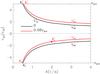 |
Fig. 2 Axial phase speed vph as a function of longitudinal
wavenumber k for a loop with profile N. The black and red
curves correspond to the static case (U0 = 0) and a case with flow
(U0 = 0.08
vA∞ and u = 100), respectively.
Here for the density parameters, a contrast of 25 and a steepness p = 100 are chosen. The
horizontal dotted line corresponds to vph = 0. The curves in the first
(fourth) quadrant are labeled |
Suppose we have a pair of propagating waves with axial wavenumbers [ k+, −
k− ] and angular frequencies
[
ω+,ω−
], where both k+ and k− are positive,
and 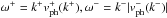 . Furthermore, we let the loop of
length L be a
segment located between z =
0 and z =
L. We will briefly explain how to construct standing
sausage modes (for details, see Li et al.2013). It was shown by Ruderman (2010) that the appropriate axial boundary condition for standing
transverse modes is that the two loop ends are two permanent nodes for the radial Lagrangian
displacement at the tube boundary, ξ(r =
a,z;t). While the rigorous derivation
therein was intended for kink modes, it also holds for standing sausage modes, which are
also transverse in nature. For ξ(r = a,z =
0;t) and ξ(r = a,z =
L;t) to be zero at arbitrary
t, one
naturally requires that ω+ = ω− =
ω, i.e.,
. Furthermore, we let the loop of
length L be a
segment located between z =
0 and z =
L. We will briefly explain how to construct standing
sausage modes (for details, see Li et al.2013). It was shown by Ruderman (2010) that the appropriate axial boundary condition for standing
transverse modes is that the two loop ends are two permanent nodes for the radial Lagrangian
displacement at the tube boundary, ξ(r =
a,z;t). While the rigorous derivation
therein was intended for kink modes, it also holds for standing sausage modes, which are
also transverse in nature. For ξ(r = a,z =
0;t) and ξ(r = a,z =
L;t) to be zero at arbitrary
t, one
naturally requires that ω+ = ω− =
ω, i.e., 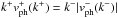 , where the phase speed for
k+
(k−) is evaluated along the branch in the
first (fourth) quadrant in Fig. 2. Consequently,
ξ(r =
a,z;t) is in the form
, where the phase speed for
k+
(k−) is evaluated along the branch in the
first (fourth) quadrant in Fig. 2. Consequently,
ξ(r =
a,z;t) is in the form 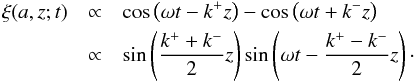 (14)One
then needs to require that
(14)One
then needs to require that 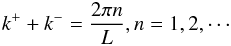 (15)in
order to meet the boundary conditions. By convention, n = 1 corresponds to the
fundamental mode, and n ≥
2 to its overtones. Throughout this manuscript, we focus on the
fundamental mode, which is important from an observational viewpoint since it yields the
longest period.
(15)in
order to meet the boundary conditions. By convention, n = 1 corresponds to the
fundamental mode, and n ≥
2 to its overtones. Throughout this manuscript, we focus on the
fundamental mode, which is important from an observational viewpoint since it yields the
longest period.
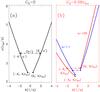 |
Fig. 3 Dependence of angular frequency ω on axial wavenumber k for both a) a static loop and b) a loop with flow. The numerical results found in Fig. 2 are adopted. The ω–k curve in the first (second) quadrant derives from the curve in the first (fourth) quadrant of Fig. 2. In panel b), the blue curves correspond to the case with a different flow profile steepness, u = 1.1. |
Figure 3 illustrates how the standing modes are
constructed in a simple graphical manner, for both (a) a static loop and (b) a loop with
flow. Here the computed results in Fig. 2 are used,
which are now converted into the ω–k space. The blue curves in Fig. 3b correspond to a different flow profile steepness, u = 1.1. They are to be
discussed in relation to Fig. 5. We note that instead
of mapping the curves in the fourth quadrant in Fig. 2
to the fourth quadrant with positive k but negative ω, we map them to the second
quadrant with negative k but positive ω. Given a loop length
L, in view of
Eq. (15) one readily finds the corresponding
k+
and k− by drawing a horizontal line in the
ω-k diagram and then measuring the separation between
the two intersections of this horizontal line with the ω+ and
ω−
curves. The fundamental mode corresponds to the case where this separation equals
2π/L (see the
horizontal dash-dotted line in Fig. 3a). Evidently, for
static loops, the ω+ and ω− curves are
symmetric with respect to the k
= 0 axis, and consequently both k+ and
k−
are simply π/L. For loops with
flow, however, for a given L one has to find k+ and
k−
numerically, given that a symmetry between the ω+ and ω− curves is no
longer present. We let  and
and
 denote the
cutoff wavenumbers in the first and fourth quadrants in Fig. 2, respectively. For static loops, one finds that (L/a)cutoff
is simply
denote the
cutoff wavenumbers in the first and fourth quadrants in Fig. 2, respectively. For static loops, one finds that (L/a)cutoff
is simply ![Mathematical equation: \hbox{$2\pi/[(k_{\rm c}^+ + k_{\rm c}^-)a] = \pi/(k_{\rm c}^+ a)$}](/articles/aa/full_html/2014/08/aa23352-13/aa23352-13-eq123.png) . However,
when U0 is not zero, then one finds that
(L/a)cutoff
is not determined by
. However,
when U0 is not zero, then one finds that
(L/a)cutoff
is not determined by ![Mathematical equation: \hbox{$2\pi/[(k_{\rm c}^+ + k_{\rm c}^-)a]$}](/articles/aa/full_html/2014/08/aa23352-13/aa23352-13-eq124.png) but by
but by
![Mathematical equation: \hbox{$2\pi/[(k_{\rm c}^+ + \bar{k}_{\rm c}^-)a]$}](/articles/aa/full_html/2014/08/aa23352-13/aa23352-13-eq125.png) , where
, where
 satisfies
  (Fig. 3b; the derived
is also given by the filled dot in Fig. 2). Evidently,
(L/a)cutoff
in this case with flow is smaller than its static counterpart. Regarding the maximum period
allowed for trapped modes, it is determined by
(Fig. 3b; the derived
is also given by the filled dot in Fig. 2). Evidently,
(L/a)cutoff
in this case with flow is smaller than its static counterpart. Regarding the maximum period
allowed for trapped modes, it is determined by  for the static and non-static
cases alike. To illustrate this point, we give some specific values. For the static case
(with parameters ρ0/ρ∞ =
25 and p =
100), we find that
for the static and non-static
cases alike. To illustrate this point, we give some specific values. For the static case
(with parameters ρ0/ρ∞ =
25 and p =
100), we find that  , while
for the non-static case (U0 = 0.08vA∞
and u = 100),
, while
for the non-static case (U0 = 0.08vA∞
and u = 100),
 and
and
 .
Consequently, for the non-static case, one finds that
.
Consequently, for the non-static case, one finds that
 ,
which is not far from the static case where Pmax =
2.5a/vA0.
However, in the non-static case
,
which is not far from the static case where Pmax =
2.5a/vA0.
However, in the non-static case  , resulting in
![Mathematical equation: \hbox{$\lacut = 2\pi/[(k_{\rm c}^+ + \bar{k}_{\rm c}^-)a] = 2.471$}](/articles/aa/full_html/2014/08/aa23352-13/aa23352-13-eq136.png) ,
which is significantly smaller than in the static case where
,
which is significantly smaller than in the static case where
 . For
comparison, the cutoff wavenumber in the static case with the same density ratio but a
discontinuous density profile,
. For
comparison, the cutoff wavenumber in the static case with the same density ratio but a
discontinuous density profile,  , and
consequently Pstep =
2.56a/vA0
and
, and
consequently Pstep =
2.56a/vA0
and  (see
Eqs.(3) to (5)). At this point, it should be pointed out that reversing the sign of
does not change the periods and cutoff loop-to-radius ratios, for in that case, the
ω–k diagrams will be a mirror-reflection of Fig. 3, with Pmax and (L/a)cutoff
determined by
(see
Eqs.(3) to (5)). At this point, it should be pointed out that reversing the sign of
does not change the periods and cutoff loop-to-radius ratios, for in that case, the
ω–k diagrams will be a mirror-reflection of Fig. 3, with Pmax and (L/a)cutoff
determined by  and
and
![Mathematical equation: \hbox{$2\pi/[(k_{\rm c}^- + \bar{k}_{\rm c}^+)a]$}](/articles/aa/full_html/2014/08/aa23352-13/aa23352-13-eq142.png) ,
respectively, where
,
respectively, where  is determined by
  . As detailed in the
Appendix in Li et al. (2013), this statement is true
as long as the ambient corona is static.
. As detailed in the
Appendix in Li et al. (2013), this statement is true
as long as the ambient corona is static.
Two things are clear from the construction procedure. First, from Eq. (14) it immediately follows that in half of each period the radial displacement at the loop boundary possesses an additional node, which moves between z = 0 and z = L. In addition, the phase of the mode depends linearly on the distance along the loop. These two signatures are not specific to sausage modes, but are common to standing modes in a loop with flow (see Fig. 1 in Terradas et al.2011 where standing kink modes are of interest). Actually, Terradas et al. (2011) demonstrated that these signatures are indeed in line with the kink modes observed with TRACE and EIT by Verwichte et al. (2010). However, their detection in sausage modes has yet to be reported. A forward modeling approach, similar to Gruszecki et al. (2012); Antolin & Van Doorsselaere (2013); and Reznikova et al. (2014), would help in elucidating the detectability of these signatures. Second, while trapped standing modes are the main concern here, one may speculate what happens when one or both propagating waves are leaky. If both of them are leaky, the resulting standing mode would be leaky as well. If one is trapped but the other leaks out by transmitting waves into the surrounding fluid, a standing mode will be unlikely; in the end, only the trapped propagating wave would survive. These aspects certainly merit a dedicated study, which is beyond the scope of the present manuscript.
3. Numerical results
We are now in a position to address how the introduction of smooth profiles, as opposed to step-function forms, affects the period of trapped standing sausage modes, and how it affects the transition line separating the trapped and leaky regimes.
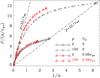 |
Fig. 4 Sausage mode period P as a function of loop length measured in units of loop radius for a loop described by profile N. The black and red curves are for the static case (flow magnitude U0 = 0) and a case with flow (U0 = 0.08 vA∞ with steepness u = 100), respectively. A density contrast of 25 is adopted. However, two values of density steepness p are examined, and given by the solid (p = 2) and dashed (p = 100) curves, respectively. The two dash-dotted lines represent the two limiting cases for static loops where the phase speed equals either the internal or the external Alfvén speed. |
Figure 4 presents the period of standing sausage modes, normalized by a/vA∞, as a function of the loop length in units of the loop radius a. As in Fig. 2, profile N is adopted for the background density and flow speed. A fixed density contrast ρ0/ρ∞ of 25 is chosen, while two values for the density profile steepness, p = 2 (the solid curves) and p = 100 (dashed), are examined. In addition to the static case (the black curves), a case with flow (red) is also examined with the flow magnitude U0 being 0.08vA∞ and flow profile steepness u being 100. Furthermore, the two dash-dotted straight lines represent 2L/vA0 and 2L/vA∞, respectively. In the static case, whichever p the density profile adopts, the period curve follows the former asymptote in the thick-tube limit (L/a ≪ 1), and terminates when intersecting the latter asymptote. This happens because the phase speed vph tends to the internal Alfvén speed vA0 when ka ≫ 1, and attains the external speed vA∞ as its maximum, beyond which sausage waves become leaky (see Fig. 2). In the case with flow, the red curves are not bounded by the two straight lines. This arises because when ka ≫ 1, the phase speed vph in the first (fourth) quadrant in Fig. 2 tends to vA0 + U0 (− vA0 + U0). At a given loop length, it can be seen that P in the case with flow is higher than its static counterpart. However, while P also increases with increasing L, the maximum period the trapped modes can reach, Pmax, does not exceed the corresponding value in the static case, for the maximum allowed loop length is substantially shorter. Despite the differences in the approaches adopted, the static computations (the black curves) agree closely with Fig. 3 in NHM12 for the trapped modes. In particular, the tendency for P to be higher for steeper density profiles means that the step-function limit Pstep (Eq. (5)) may be the upper limit to the period that trapped modes may attain when profile N is adopted. We note that for profile E, the same tendency for P to increase monotonically with L also holds, for static and non-static loops alike. However, showing the relevant curves would make the graph too crowded and therefore we have omitted them.
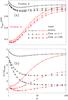 |
Fig. 5 Dependence on density profile steepness p of a) the maximum sausage period Pmax and b) the threshold length-to-radius ratio (L/a)cutoff. The black (red) curves are for loops described by profile E (N). A density contrast of 25 is adopted. The solid curves corresponds to the static case (flow magnitude U0 = 0), while the dotted and dashed lines correspond to the cases with flow where the flow profile steepness u is 1.1 and 100, respectively. In the cases with flow, U0 is fixed at 0.08 vA∞. |
How does the maximum period Pmax depend on the density profile
steepness p?
Will it exceed Pstep if a different profile is chosen or in
some particular range of p? This is examined in Fig. 5a where the profiles N (the red curves) and E (black) are plotted, and
where Pmax/Pstep
instead of Pmax is shown as a function of
p. Here the
density contrast ρ0/ρ∞
is fixed at 25. In addition, the
case with a fixed flow magnitude U0 = 0.08vA∞
is represented by the dotted and dashed curves, corresponding to a flow profile steepness
u of
1.1 and 100, respectively. For other choices of
u, the
results lie in between. Several points are clear from Fig. 5a. First, for both profiles the effect of flow profile steepness on
Pmax is marginal: while Pmax slightly
decreases with increasing u at a given p, Pmax in the case u = 100 is smaller than
Pmax for u = 1.1 by only a few
percent. Moreover, Pmax in the case with flow is always
smaller than its static counterpart for all the examined density profile steepnesses, which
is also true for both profiles. Second, for profile E the maximum period Pmax is
insensitive to the density profile steepness p. In contrast, for profile N Pmax shows a
remarkably sensitive p-dependence. In the static case, for instance, with
p ranging
from 1 to 100, Pmax for profile E
varies by ≲12%; however,
Pmax/Pstep
for profile N increases considerably from 0.37 at p ~
1 to 0.98
when p = 100.
Third, one can see that for both profiles the dependence on p of Pmax is not
monotonic. In the static case for profile E, for example, with p increasing from
1, Pmax decreases
rather than increasing first to a local minimum at p ≈ 2.5 before rising again.
The same non-monotonic behavior also takes place for profile N, although the variation in
Pmax at small p appears too shallow to
distinguish. The peculiar p-dependence is closely related to the p-dependence of
 , given that
Pmax is determined by
.
, given that
Pmax is determined by
.
The trapping capabilities of loops are more clearly shown by Fig. 5b where the cutoff length-to-radius ratio (L/a)cutoff
is plotted. With the rest of the parameters chosen, this (L/a)cutoff
is the maximum value a loop can have for it to support trapped standing sausage modes. We
consider static loops first. One can see that for both profiles, the way in which
(L/a)cutoff
depends on the density profile steepness p is identical to how the maximal period
Pmax behaves, which is not surprising given
that Pmax =
2(L/a)cutoff(a/vA∞).
In a more intuitive way, the behavior of (L/a)cutoff
indicates that for profile N, the general tendency is that the steeper the profile, the
better a loop can trap sausage modes, in close agreement with NHM12. However, for profile E,
that a loop has a steeper density distribution does not necessarily mean it is a better
waveguide for sausage modes. Now we consider non-static loops, for which one can see that
for both profiles, relative to the static case, introducing a flow with a magnitude of
merely 0.08
vA∞ substantially reduces (L/a)cutoff
at any given p.
This reduction is particularly prominent for large values of p. Moreover, while the effect
of the flow profile steepness u is marginal as far as the maximum period is
concerned, it is substantial in determining the maximum loop-to-radius ratio, with the
tendency for both profiles being that (L/a)cutoff
decreases with increasing u. For profile N (the red curves), for instance, when
p = 100,
(L/a)cutoff
reads 6.25 in the static case,
and reads 4.17 (2.47) when u = 1.1 (100) in the non-static case. The apparently
unexpected behavior for steeper density or flow profiles to yield less strong trapping in
certain cases derives from the intricate p- or u- dependence of the cutoff wavenumber
and its
combination with
(see Fig. 2). As illustrated by the red
(u = 100) and
blue (u = 1.1)
curves in Fig. 3, with increasing u the ω-k curves in the first and
second quadrants become increasingly asymmetric. While the
values are
similar in the two cases, the stronger asymmetry for u = 100 results in a
that is substantially larger. We consider profile N and p = 100, for example, to
examine the peculiar u-dependence. When u = 1.1, one finds that
 and
and
 . However, when u = 100, one finds that
 and
and
 read 0.549
/a and 1.994 /a,
respectively.
read 0.549
/a and 1.994 /a,
respectively.
Figure 5a has a number of important implications for interpreting the quasi-periodic oscillations in flare lightcurves. First, the period analytically derived for a piece-wise constant density profile (the step-function case, Eq. (5)) can be taken as an upper limit for the periods that standing sausage modes can attain. This is true regardless of the particular density profile or whether a loop flow exists, meaning that these two complications do not broaden the period range of the quasi-periodic oscillations that can be attributed to sausage modes. Second, the seismological tool to probe the transverse density profile steepness, which was proposed in NHM12 and capitalizes on the sensitive dependence on the density profile steepness of the maximum period, requires that the density profile be more properly described by profile N rather than profile E. Given the importance of obtaining the information on the transverse fine structuring, we conclude that there is an imperative need to observationally distinguish between the two profiles.
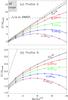 |
Fig. 6 Dependence on density contrast ρ0/ρ∞ of threshold length-to-radius ratio (L/a)cutoff below which standing sausage modes are trapped. Both a) profile E and b) profile N are examined. The solid black curves are for the static case, while the colored curves represent the non-static cases with the flow magnitude U0 ranging from 0.02 vA∞ to 0.08 vA∞. In the computations, both the density and flow profile steepness, p and u, are taken to be 2. The dashed straight lines in both panels represent the threshold length-to-radius ratio analytically derived in the static case for a step-function profile (Eq. (4)). Furthermore, the hatched area corresponds to the parameter range for typical active region (AR) loops. The horizontal dashed line represents the length-to-radius ratio of the flaring loop reported in Nakariakov et al. (2003). |
We can now further examine the parameter range where trapped sausage modes are allowed.
This is done in Fig. 6 which plots the maximum
length-to-radius ratio (L/a)cutoff
as a function of density contrast ρ0/ρ∞,
or more precisely the Alfvén speed ratio  ,
for both profiles E (upper panel) and N (lower), and for both static (black) and non-static
(colored) cases. A series of values for the flow magnitude is presented, with
U0
ranging from 0.02
vA∞ to 0.08 vA∞. For
illustrative purposes, the values for the density and flow profile steepness,
p and
u, are both
chosen to be 2. In addition, the
dashed lines in both panels represent (L/a)cutoff
(Eq. (4)) attained in the step-function limit
for static loops for comparison. Each curve divides the L/a–ρ0/ρ∞
space into two regions, with trapped sausage modes permitted (prohibited) to its right
(left). While similar in format to Fig. 2 in Aschwanden et
al. (2004) where a density profile of step-function form is used, here the effects
of both a smooth transverse profile and the presence of a loop flow are included. One can
see that with the chosen p, for static loops with profile E, the cutoff
length-to-radius ratio (the black solid curve in Fig. 6a) does not differ significantly from the step-function limit (the dashed line),
whereas for static loops with profile N, (L/a)cutoff
is substantially smaller, with the deviation increasing with the density contrast (Fig.
6b). Furthermore, introducing a loop flow leads to a
reduction in (L/a)cutoff
in general. In particular, for both profiles E and N, when U0 exceeds
~0.04 vA∞, the
dependence of (L/a)cutoff
on ρ0/ρ∞
is not monotonic, but attains a maximum. We examine what this means for flaring loops, for
which we plot the horizontal dashed line in Fig. 6a
corresponding to L/a = 25 Mm / 3
Mm, taken from NMR03 and seen as being representative. One can see that
for profile E, a density contrast is required to exceed ~45.6 (60.8) for loops with U0 being
0 (0.02 vA∞) to host
trapped sausage modes. When U0 ≳ 0.04 vA∞,
however, the horizontal dashed line does not intersect the corresponding colored curves,
meaning that if a flow with such a magnitude was present in the flaring loop analysed in
NMR03, the sausage mode would be in the leaky regime. We note that this flow magnitude is
not unrealistic: taking vA∞ to ~3300 km s-1 derived for this particular
event (Melnikov et al. 2005), one finds that
evaluating 0.04vA∞ yields ~130 km s-1. As for profile N, even in
the case of static loops, for them to trap standing sausage modes, it turns out that
ρ0/ρ∞
has to exceed ~2970, which seems
large even for flaring loops and is actually beyond the horizontal range used to plot Fig.
6. Hence, if profile N more accurately describes the
density profile of the flaring loop considered in NMR03, then the standing mode identified
therein should be a leaky one.
,
for both profiles E (upper panel) and N (lower), and for both static (black) and non-static
(colored) cases. A series of values for the flow magnitude is presented, with
U0
ranging from 0.02
vA∞ to 0.08 vA∞. For
illustrative purposes, the values for the density and flow profile steepness,
p and
u, are both
chosen to be 2. In addition, the
dashed lines in both panels represent (L/a)cutoff
(Eq. (4)) attained in the step-function limit
for static loops for comparison. Each curve divides the L/a–ρ0/ρ∞
space into two regions, with trapped sausage modes permitted (prohibited) to its right
(left). While similar in format to Fig. 2 in Aschwanden et
al. (2004) where a density profile of step-function form is used, here the effects
of both a smooth transverse profile and the presence of a loop flow are included. One can
see that with the chosen p, for static loops with profile E, the cutoff
length-to-radius ratio (the black solid curve in Fig. 6a) does not differ significantly from the step-function limit (the dashed line),
whereas for static loops with profile N, (L/a)cutoff
is substantially smaller, with the deviation increasing with the density contrast (Fig.
6b). Furthermore, introducing a loop flow leads to a
reduction in (L/a)cutoff
in general. In particular, for both profiles E and N, when U0 exceeds
~0.04 vA∞, the
dependence of (L/a)cutoff
on ρ0/ρ∞
is not monotonic, but attains a maximum. We examine what this means for flaring loops, for
which we plot the horizontal dashed line in Fig. 6a
corresponding to L/a = 25 Mm / 3
Mm, taken from NMR03 and seen as being representative. One can see that
for profile E, a density contrast is required to exceed ~45.6 (60.8) for loops with U0 being
0 (0.02 vA∞) to host
trapped sausage modes. When U0 ≳ 0.04 vA∞,
however, the horizontal dashed line does not intersect the corresponding colored curves,
meaning that if a flow with such a magnitude was present in the flaring loop analysed in
NMR03, the sausage mode would be in the leaky regime. We note that this flow magnitude is
not unrealistic: taking vA∞ to ~3300 km s-1 derived for this particular
event (Melnikov et al. 2005), one finds that
evaluating 0.04vA∞ yields ~130 km s-1. As for profile N, even in
the case of static loops, for them to trap standing sausage modes, it turns out that
ρ0/ρ∞
has to exceed ~2970, which seems
large even for flaring loops and is actually beyond the horizontal range used to plot Fig.
6. Hence, if profile N more accurately describes the
density profile of the flaring loop considered in NMR03, then the standing mode identified
therein should be a leaky one.
Figure 6 also allows us to say a few words on active region (AR) loops, for which the combination of typical length-to-radius ratios L/a and density contrasts ρ0/ρ∞ corresponds to the hatched area in Fig. 6a. We note that L/a is typically ≲0.05 (Table 1 in Ofman & Aschwanden2002, also Fig. 1 in Schrijver2007), but is taken here to be ≲0.1 for safety. The density contrast of AR loops relative to their ambient is difficult to yield; nevertheless, a range of 2 to 10 is often quoted. From Fig. 6a and b one expects that AR loops do not support trapped sausage modes: in the case of profile E, the hatched area is far from all the curves; in the case of profile N, it is beyond the range in which the curves are plotted. Moreover, because of their mild density contrast, AR loops are unlikely to support observable leaky modes either because, as estimated by Zaitsev & Stepanov (1975; also Eq. (6) in Kopylova et al.2007) for static loops with a step-function density distribution, in the thin-tube limit the ratio of the damping time to wave period τ/P is approximately (ρ0/ρe)/π2, which evaluates to ≲1 for AR loops. Damped oscillations with such low-quality factors would be difficult to detect.
4. Summary
The present work is motivated by two series of studies in the context of coronal seismology. First, while ubiquitous in coronal loops in general (Aschwanden 2004) and found in a number of oscillating loops in particular (Ofman & Wang 2008), field-aligned loop flows seem to have received insufficient attention regarding their effects on the standing sausage modes. Second, widely accepted to account for second-scale quasi-periodic oscillations in solar flare lightcurves, sausage modes have been shown recently by Nakariakov et al. (2012) to offer an additional diagnostic capability for inferring how steep the transverse density profile is. The inference of the profile was made possible through the sensitive dependence of the sausage mode period on the density profile steepness. We therefore are interested in assessing the combined effects of a field-aligned loop flow as well as smooth transverse density and flow profiles on the characteristics of standing sausage modes. To this end, we work in the framework of zero-beta ideal MHD and examine the linear sausage waves trapped in straight cylinders with field-aligned flow and enhanced density embedded in a uniform magnetic field. Formulating the problem as a standard eigen-value problem, we examine the dispersion diagrams and describe the procedure for constructing standing sausage modes. In addition, we distinguish between two profiles, E and N, both of which provide a smooth distribution connecting the values at loop axis (subscript 0) and those at distances far from the loop (subscript ∞). The end result is that, the maximum period Pmax that trapped standing modes may attain, and the cutoff length-to-radius ratio (L/a)cutoff that a loop is allowed to reach for sausage modes to be trapped, depend on the choice of the transverse profiles and a combination of dimensionless parameters [ρ0/ρ∞,p; U0/vA∞,u]. Here p denotes the density profile steepness, while ρ0/ρ∞ is the density contrast of the loop relative to its surroundings. In addition, U0 is the flow magnitude, vA∞ is the external Alfvén speed, and u the flow profile steepness. For both profiles, the larger p or u, the closer the profiles are to a step-function form. Our main results are summarized as follows.
For both profiles, the sausage mode period P increases with increasing loop length. Even though (at a given loop length) P in the non-static case is higher than in the static case, the maximum period Pmax never exceeds its static counterpart because the cutoff length-to-radius ratio is substantially smaller. For either profile, with a flow magnitude U0 ≲ 0.08 vA∞, the maximum period Pmax is not substantially affected by the flow profile steepness u, although u varies significantly from ~1 to 100. The analytically expected sausage mode period for static loops with a step-function density profile can be taken as an upper limit that sausage modes can attain in the trapped regime even for loops with smooth profiles and accompanied by field-aligned flows. Consequently, incorporating these two factors into sausage mode studies does not broaden the period range for the quasi-periodic oscillations in flare lightcurves that sausage modes can be responsible for. The maximum sausage period Pmax is sensitive to the density profile steepness p if profile N is adopted to describe coronal loops, meaning that period measurements can be used to infer the information on fine structuring in this case. However, when profile E is adopted, the dependence of Pmax on p is rather insensitive. In this sense, observationally distinguishing between the two profiles is crucial for establishing Pmax as a seismological tool for this purpose.
By far the most important effect a flow introduces is to reduce the ability of coronal loops to trap sausage modes: it lowers the cutoff length-to-radius ratio (L/a)cutoff considerably compared to the static case. The flow profile steepness u is also important in this sense: (L/a)cutoff tends to decrease with increasing u. Examining the parameter space subtended by length-to-radius ratio and density contrast, Fig. 6 shows that typical active region loops do not support trapped sausage modes, and are unlikely to support leaky modes with observable quality factors given their mild density contrast. The fundamental sausage mode identified in the flaring loop reported by Nakariakov et al. (2003) is likely to be a leaky one if profile N with p = 2 (similar to a Gaussian) describes the transverse density distribution. This can also be said for profile E with p = 2 when a flow with a magnitude stronger than ~130 km s-1 was present in the loop.
Online material
Appendix A: A validation study of the BVPSUITE code
The eigen-value problem solver BVPSUITE seems new in the context of coronal seismology, hence a study validating its accuracy seems in order. To this end, we carry out a series of computations in both slab and cylindrical geometries, and compare the numerically derived dispersion curves with available analytic expectations. Given that these analytic expressions are derived in the limit of zero-beta MHD, we focus on the same situation accordingly.
We start with the slab geometry and consider the static case. The magnetic slab and the
uniform equilibrium magnetic field
are both aligned with the z-axis. The equilibrium density
is structured in the x-direction. We consider only the two-dimensional
propagation in the x-z plane. It then follows from the zero-beta MHD
equations that the eigen-value problem for fast waves in the static case can be
formulated as (e.g., Eq. (3) in Terradas et al.
2005) ![Mathematical equation: \appendix \setcounter{section}{1} \begin{eqnarray} \vph^2\tilde{b}_x(x)=-\frac{v^2_{\rm A}(x)}{k^2} \left[\frac{\mathrm{d}^2}{\mathrm{d}x^2}-k^2\right]\tilde{b}_x(x) , \label{eq_eigen_slab_bx} \end{eqnarray}](/articles/aa/full_html/2014/08/aa23352-13/aa23352-13-eq190.png) (A.1)together
with the boundary conditions
(A.1)together
with the boundary conditions 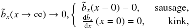 (A.2)where
sausage and kink waves differ in their behavior at the slab axis (x = 0). For the symmetric
Epstein profile
(A.2)where
sausage and kink waves differ in their behavior at the slab axis (x = 0). For the symmetric
Epstein profile  it
is possible to solve the dispersion relation analytically for the phase speed
vph (Cooper et al. 2003; MacNamara &
Roberts 2011). For kink waves, it reads
it
is possible to solve the dispersion relation analytically for the phase speed
vph (Cooper et al. 2003; MacNamara &
Roberts 2011). For kink waves, it reads 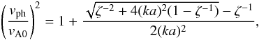 (A.3)and
for sausage waves, it reads
(A.3)and
for sausage waves, it reads  (A.4)where
ζ
represents the density contrast ρ0/ρ∞.
Figure A.1 compares the dispersion diagram computed
with BVPSUITE (the asterisks) with the analytic expressions (the dashed red curves) for
a representative density contrast ρ0/ρ∞
being 5. The internal and
external Alfvén speed, vA0 and vA∞, are
represented by the two horizontal dash-dotted lines. It can be seen that the analytic
results are exactly reproduced. In fact, we have carried out a series of comparisons
covering an extensive range of density ratios, and found exact agreement without
exception.
(A.4)where
ζ
represents the density contrast ρ0/ρ∞.
Figure A.1 compares the dispersion diagram computed
with BVPSUITE (the asterisks) with the analytic expressions (the dashed red curves) for
a representative density contrast ρ0/ρ∞
being 5. The internal and
external Alfvén speed, vA0 and vA∞, are
represented by the two horizontal dash-dotted lines. It can be seen that the analytic
results are exactly reproduced. In fact, we have carried out a series of comparisons
covering an extensive range of density ratios, and found exact agreement without
exception.
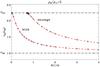 |
Fig. A.1 Dependence on the longitudinal wavenumber k of the phase speed vph for a static cold slab with a symmetric Epstein density profile. The asterisks represent the results obtained with BVPSUITE by numerically solving the eigen-value problem, while the dashed red lines represent the analytic results, Eqs. (A.3) and (A.4). Here a density ratio ρ0/ρ∞ of 5 is adopted. |
We now move on to the cylindrical case, but still restrict ourselves to the static case
for the moment. We solve the same eigen-value problem in the text, Eqs. (12) and (13), but now take the background flow
to be zero. In addition, we take p to be infinity, corresponding to a
discontinuous distribution of the equilibrium density. To facilitate the validation
study, we focus on sausage waves given the availability of their analytic behavior both
in the neighborhood of the cutoff wavenumber and for large wavenumbers. In the former,
the dispersion behavior in terms of angular frequency ω can be expressed as
(Eq. (53) in Vasheghani Farahani et al. 2014)
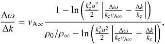 (A.5)where
Δω = ω −
kcvA∞,
Δk = k −
kc, and kc is the
cutoff wavenumber given by Eq. (3). For
Eq. (A.5) to be valid, one nominally
requires that Δk/kc ≪
1. On the other hand, when ka ≫ 1, the dispersion relation Eq. (8b) in Edwin & Roberts (1983) can be shown to yield
(A.5)where
Δω = ω −
kcvA∞,
Δk = k −
kc, and kc is the
cutoff wavenumber given by Eq. (3). For
Eq. (A.5) to be valid, one nominally
requires that Δk/kc ≪
1. On the other hand, when ka ≫ 1, the dispersion relation Eq. (8b) in Edwin & Roberts (1983) can be shown to yield
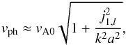 (A.6)where
j1,l (l =
1,2,··· ) denotes the
l-th zero
of J1 and l denotes the infinite
number of sausage branches. For the first branch we compute, j1,1 =
3.83.
(A.6)where
j1,l (l =
1,2,··· ) denotes the
l-th zero
of J1 and l denotes the infinite
number of sausage branches. For the first branch we compute, j1,1 =
3.83.
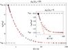 |
Fig. A.2 Similar to Fig. A.1 but for sausage waves supported by static cylinders with discontinuous density distribution. The dashed red curves represent the analytic results in the vicinity of the cutoff wavenumber (Eq. (A.5)) and for big wavenumbers (Eq. (A.6)). Here two density ratios, 4 and 25, are adopted. |
Figure A.2 presents the dispersion curves expressing the phase speed vph as a function of longitudinal wavenumber k. For illustrative purposes, we present the results for two density contrasts, one large (ρ0/ρ∞ = 25) and the other rather mild (ρ0/ρ∞ = 4, inset). The results computed with BVPSUITE are given by the asterisks, and the analytic results are represented by the red dashed curves. The two horizontal dash-dotted lines represent the internal and external Alfvén speeds. Evidently, the numerical results excellently capture the cutoff wavenumber, and agree remarkably well with the analytic results for the appropriate wavenumber ranges. Actually, this can be said for all the tests we performed, which cover an extensive range of density ratios.
Our next validation study pertains to sausage waves supported by cold cylinders with
flow. To this end we start with the comprehensive study by Goossens et al. (1992) where the sophisticated equilibrium
configuration takes account of a background flow, and azimuthal components of the
equilibrium velocity and magnetic field. By neglecting these azimuthal components and
specializing to a piece-wise constant distribution for both the equilibrium density and
flow speed, one finds that Eq. (18) in Goossens et al.
(1992) simplifies to  (A.7)where
 denotes the Fourier amplitude of the total pressure perturbation. Equation (A.7) is valid both inside and outside the
cylinder, and m2 is defined as
denotes the Fourier amplitude of the total pressure perturbation. Equation (A.7) is valid both inside and outside the
cylinder, and m2 is defined as
 in
which we have assumed that the ambient corona is static. For the simple configuration in
question, Eq. (A.7) is analytically
solvable in terms of Bessel function J0 (K0) inside
(outside) the cylinder for trapped modes. A dispersion relation then follows from the
continuity of the transverse Lagrangian displacement and total pressure perturbation at
the cylinder boundary (see also, e.g., Terra-Homem et
al. 2003),
in
which we have assumed that the ambient corona is static. For the simple configuration in
question, Eq. (A.7) is analytically
solvable in terms of Bessel function J0 (K0) inside
(outside) the cylinder for trapped modes. A dispersion relation then follows from the
continuity of the transverse Lagrangian displacement and total pressure perturbation at
the cylinder boundary (see also, e.g., Terra-Homem et
al. 2003), ![Mathematical equation: \appendix \setcounter{section}{1} \begin{equation} \rhoinf \left(\vainf^2 - \vph^2\right) n_0 \frac{J_0'(n_0 a)}{J_0(n_0 a)} = \rho_0 \left[\vain^2 - (\vph\! -\! U_0)^2\right] m_\infty \frac{K_0'(m_\infty a)}{K_0(m_\infty a)} , \label{eq_vali_cyl_flow_disp} \end{equation}](/articles/aa/full_html/2014/08/aa23352-13/aa23352-13-eq216.png) (A.8)where
(A.8)where
 .
Furthermore, the prime denotes the derivative of Bessel function with respect to its
argument, e.g.,
.
Furthermore, the prime denotes the derivative of Bessel function with respect to its
argument, e.g.,  with
η =
m∞a.
with
η =
m∞a.
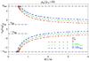 |
Fig. A.3 Dependence on the longitudinal wavenumber k of the phase speed vph for a cold cylinder with flow where the transverse distributions of both the equilibrium density and field-aligned flow adopt a step-function form. The asterisks represent the results obtained with BVPSUITE by numerically solving the eigen-value problem, while the dashed lines represent the solution to the analytically derived dispersion relation (Eq. (A.8)). The horizontal dash-dotted lines correspond to the internal and external Alfvén speeds. Here three different values of the internal flow speed U0 are examined for a density ratio ρ0/ρ∞ being 25. |
Figure A.3 presents the dependence of the phase speed vph on the axial wavenumber k for a representative density
contrast ρ0/ρ∞ being 25. For illustrative purposes, we examine three values of the internal flow speed U0, namely, 0 (red), 0.08 (green), and 0.16 (blue) times the external Alfvén speed vA∞. The horizontal dash-dotted lines represent the internal and external Alfvén speeds. The asterisks give the results from solving Eqs.(12) and (13) in the text with BVPSUITE, where both the density and flow speed profile steepnesses, p and u, are taken to be infinity. For comparison, the dashed curves represent the solutions to the algebraic dispersion relation, Eq. (A.8). One can see that the two sets of solutions agree with each other remarkably well. As a matter of fact, the agreement is found for all the tests we conducted, where we examined an extensive range of density contrasts and flow magnitudes.
In closing, we mention that at this stage of its development, the Matlab eigen-value problem solver BVPSUITE cannot find complex eigen-values, thereby limiting its use to trapped modes. Despite this, given that BVPSUITE is publicly available and easy to use with its friendly graphical user interface, this accurate code may find a wider application to problems encountered in coronal seismology.
Acknowledgments
We thank the referee for his/her valuable comments, which helped improve this manuscript substantially. This research is supported by the 973 program 2012CB825601, National Natural Science Foundation of China (40904047, 41174154, 41274176, and 41274178), the Ministry of Education of China (20110131110058 and NCET-11-0305), and by the Provincial Natural Science Foundation of Shandong via grant JQ201212.
References
- Antolin, P., & Van Doorsselaere, T. 2013, A&A, 555, A74 [NASA ADS] [CrossRef] [EDP Sciences] [Google Scholar]
- Aschwanden, M. J. 2004, Physics of the Solar Corona (Berlin: Springer-Verlag) [Google Scholar]
- Aschwanden, M. J., Nakariakov, V. M., & Melnikov, V. F. 2004, ApJ, 600, 458 [NASA ADS] [CrossRef] [Google Scholar]
- Ballester, J. L., Erdélyi, R., Hood, A. W., Leibacher, J. W., & Nakariakov, V. M. 2007, Sol. Phys., 246, 1 [NASA ADS] [CrossRef] [Google Scholar]
- Banerjee, D., Erdélyi, R., Oliver, R., & O’Shea, E. 2007, Sol. Phys., 246, 3 [NASA ADS] [CrossRef] [Google Scholar]
- Chen, S.-X., Li, B., Xia, L.-D., Chen, Y.-J., & Yu, H. 2013, Sol. Phys., 270 [Google Scholar]
- Cooper, F. C., Nakariakov, V. M., & Tsiklauri, D. 2003, A&A, 397, 765 [NASA ADS] [CrossRef] [EDP Sciences] [Google Scholar]
- De Moortel, I., & Nakariakov, V. M. 2012, Roy. Soc. London Philos. Trans. Ser. A, 370, 3193 [Google Scholar]
- Del Zanna, G. 2008, A&A, 481, L49 [NASA ADS] [CrossRef] [EDP Sciences] [Google Scholar]
- Edwin, P. M., & Roberts, B. 1983, Sol. Phys., 88, 179 [NASA ADS] [CrossRef] [Google Scholar]
- Erdélyi, R., & Goossens, M. 2011, Space Sci. Rev., 158, 167 [NASA ADS] [CrossRef] [Google Scholar]
- Goossens, M., Hollweg, J. V., & Sakurai, T. 1992, Sol. Phys., 138, 233 [NASA ADS] [CrossRef] [Google Scholar]
- Gruszecki, M., Murawski, K., & Ofman, L. 2008, A&A, 488, 757 [NASA ADS] [CrossRef] [EDP Sciences] [Google Scholar]
- Gruszecki, M., Nakariakov, V. M., & Van Doorsselaere, T. 2012, A&A, 543, A12 [NASA ADS] [CrossRef] [EDP Sciences] [Google Scholar]
- Inglis, A. R., Nakariakov, V. M., & Melnikov, V. F. 2008, A&A, 487, 1147 [NASA ADS] [CrossRef] [EDP Sciences] [Google Scholar]
- Inglis, A. R., Van Doorsselaere, T., Brady, C. S., & Nakariakov, V. M. 2009, A&A, 503, 569 [NASA ADS] [CrossRef] [EDP Sciences] [Google Scholar]
- Kitzhofer, G., Koch, O., & Weinmüller, E. 2009, AIP Conf. Proc., 1168, 39 [NASA ADS] [CrossRef] [Google Scholar]
- Kopylova, Y. G., Melnikov, A. V., Stepanov, A. V., Tsap, Y. T., & Goldvarg, T. B. 2007, Astron. Lett., 33, 706 [NASA ADS] [CrossRef] [Google Scholar]
- Lemen, J. R., Title, A. M., Akin, D. J., et al. 2012, Sol. Phys., 275, 17 [NASA ADS] [CrossRef] [Google Scholar]
- Li, B., Habbal, S. R., & Chen, Y. 2013, ApJ, 767, 169 [NASA ADS] [CrossRef] [Google Scholar]
- MacNamara, C. K., & Roberts, B. 2011, A&A, 526, A75 [NASA ADS] [CrossRef] [EDP Sciences] [Google Scholar]
- Melnikov, V. F., Reznikova, V. E., Shibasaki, K., & Nakariakov, V. M. 2005, A&A, 439, 727 [NASA ADS] [CrossRef] [EDP Sciences] [Google Scholar]
- Morton, R. J., Verth, G., Jess, D. B., et al. 2012, Nature Comm., 3, 1315, [Google Scholar]
- Nakariakov, V. M., & Erdélyi, R. 2009, Space Sci. Rev., 149, 1 [NASA ADS] [CrossRef] [Google Scholar]
- Nakariakov, V. M., & Melnikov, V. F. 2009, Space Sci. Rev., 149, 119 [NASA ADS] [CrossRef] [Google Scholar]
- Nakariakov, V. M., & Roberts, B. 1995, Sol. Phys., 159, 399 [NASA ADS] [CrossRef] [Google Scholar]
- Nakariakov, V. M., Melnikov, V. F., & Reznikova, V. E. 2003, A&A, 412, L7 [NASA ADS] [CrossRef] [EDP Sciences] [Google Scholar]
- Nakariakov, V. M., Hornsey, C., & Melnikov, V. F. 2012, ApJ, 761, 134 [NASA ADS] [CrossRef] [Google Scholar]
- Ofman, L., & Aschwanden, M. J. 2002, ApJ, 576, L153 [NASA ADS] [CrossRef] [Google Scholar]
- Ofman, L., & Wang, T. J. 2008, A&A, 482, L9 [NASA ADS] [CrossRef] [EDP Sciences] [Google Scholar]
- Pascoe, D. J., Nakariakov, V. M., & Arber, T. D. 2007a, A&A, 461, 1149 [NASA ADS] [CrossRef] [EDP Sciences] [Google Scholar]
- Pascoe, D. J., Nakariakov, V. M., & Arber, T. D. 2007b, Sol. Phys., 246, 165 [NASA ADS] [CrossRef] [Google Scholar]
- Pascoe, D. J., Nakariakov, V. M., Arber, T. D., & Murawski, K. 2009, A&A, 494, 1119 [NASA ADS] [CrossRef] [EDP Sciences] [Google Scholar]
- Pesnell, W. D., Thompson, B. J., & Chamberlin, P. C. 2012, Sol. Phys., 275, 3 [NASA ADS] [CrossRef] [Google Scholar]
- Reznikova, V. E., Antolin, P., & Van Doorsselaere, T. 2014, ApJ, 785, 86 [NASA ADS] [CrossRef] [Google Scholar]
- Roberts, B. 2000, Sol. Phys., 193, 139 [NASA ADS] [CrossRef] [Google Scholar]
- Roberts, B., Edwin, P. M., & Benz, A. O. 1984, ApJ, 279, 857 [NASA ADS] [CrossRef] [Google Scholar]
- Rosenberg, H. 1970, A&A, 9, 159 [NASA ADS] [Google Scholar]
- Ruderman, M. S. 2010, Sol. Phys., 267, 377 [NASA ADS] [CrossRef] [Google Scholar]
- Schrijver, C. J. 2007, ApJ, 662, L119 [NASA ADS] [CrossRef] [Google Scholar]
- Su, J. T., Shen, Y. D., Liu, Y., Liu, Y., & Mao, X. J. 2012, ApJ, 755, 113 [NASA ADS] [CrossRef] [Google Scholar]
- Terra-Homem, M., Erdélyi, R., & Ballai, I. 2003, Sol. Phys., 217, 199 [NASA ADS] [CrossRef] [Google Scholar]
- Terradas, J., Oliver, R., & Ballester, J. L. 2005, A&A, 441, 371 [NASA ADS] [CrossRef] [EDP Sciences] [Google Scholar]
- Terradas, J., Arregui, I., Verth, G., & Goossens, M. 2011, ApJ, 729, L22 [NASA ADS] [CrossRef] [Google Scholar]
- Tripathi, D., Mason, H. E., Del Zanna, G., & Bradshaw, S. 2012, ApJ, 754, L4 [NASA ADS] [CrossRef] [Google Scholar]
- Uchida, Y. 1970, PASJ, 22, 341 [NASA ADS] [Google Scholar]
- Van Doorsselaere, T., Verwichte, E., & Terradas, J. 2009, Space Sci. Rev., 149, 299 [NASA ADS] [CrossRef] [Google Scholar]
- Van Doorsselaere, T., De Groof, A., Zender, J., Berghmans, D., & Goossens, M. 2011, ApJ, 740, 90 [NASA ADS] [CrossRef] [Google Scholar]
- Vasheghani Farahani, S., Hornsey, C., Van Doorsselaere, T., & Goossens, M. 2014, ApJ, 781, 92 [NASA ADS] [CrossRef] [Google Scholar]
- Verwichte, E., Foullon, C., & Van Doorsselaere, T. 2010, ApJ, 717, 458 [NASA ADS] [CrossRef] [Google Scholar]
- Zaitsev, V. V., & Stepanov, A. V. 1975, Issledovaniia Geomagnetizmu Aeronomii i Fizike Solntsa, 37, 3 [NASA ADS] [Google Scholar]
- Zaitsev, V. V., & Stepanov, A. V. 1982, Sov. Astron. Lett., 8, 132 [NASA ADS] [Google Scholar]
All Figures
|
Fig. 1 Background density |
| In the text | |
|
Fig. 2 Axial phase speed vph as a function of longitudinal
wavenumber k for a loop with profile N. The black and red
curves correspond to the static case (U0 = 0) and a case with flow
(U0 = 0.08
vA∞ and u = 100), respectively.
Here for the density parameters, a contrast of 25 and a steepness p = 100 are chosen. The
horizontal dotted line corresponds to vph = 0. The curves in the first
(fourth) quadrant are labeled |
| In the text | |
|
Fig. 3 Dependence of angular frequency ω on axial wavenumber k for both a) a static loop and b) a loop with flow. The numerical results found in Fig. 2 are adopted. The ω–k curve in the first (second) quadrant derives from the curve in the first (fourth) quadrant of Fig. 2. In panel b), the blue curves correspond to the case with a different flow profile steepness, u = 1.1. |
| In the text | |
|
Fig. 4 Sausage mode period P as a function of loop length measured in units of loop radius for a loop described by profile N. The black and red curves are for the static case (flow magnitude U0 = 0) and a case with flow (U0 = 0.08 vA∞ with steepness u = 100), respectively. A density contrast of 25 is adopted. However, two values of density steepness p are examined, and given by the solid (p = 2) and dashed (p = 100) curves, respectively. The two dash-dotted lines represent the two limiting cases for static loops where the phase speed equals either the internal or the external Alfvén speed. |
| In the text | |
|
Fig. 5 Dependence on density profile steepness p of a) the maximum sausage period Pmax and b) the threshold length-to-radius ratio (L/a)cutoff. The black (red) curves are for loops described by profile E (N). A density contrast of 25 is adopted. The solid curves corresponds to the static case (flow magnitude U0 = 0), while the dotted and dashed lines correspond to the cases with flow where the flow profile steepness u is 1.1 and 100, respectively. In the cases with flow, U0 is fixed at 0.08 vA∞. |
| In the text | |
|
Fig. 6 Dependence on density contrast ρ0/ρ∞ of threshold length-to-radius ratio (L/a)cutoff below which standing sausage modes are trapped. Both a) profile E and b) profile N are examined. The solid black curves are for the static case, while the colored curves represent the non-static cases with the flow magnitude U0 ranging from 0.02 vA∞ to 0.08 vA∞. In the computations, both the density and flow profile steepness, p and u, are taken to be 2. The dashed straight lines in both panels represent the threshold length-to-radius ratio analytically derived in the static case for a step-function profile (Eq. (4)). Furthermore, the hatched area corresponds to the parameter range for typical active region (AR) loops. The horizontal dashed line represents the length-to-radius ratio of the flaring loop reported in Nakariakov et al. (2003). |
| In the text | |
|
Fig. A.1 Dependence on the longitudinal wavenumber k of the phase speed vph for a static cold slab with a symmetric Epstein density profile. The asterisks represent the results obtained with BVPSUITE by numerically solving the eigen-value problem, while the dashed red lines represent the analytic results, Eqs. (A.3) and (A.4). Here a density ratio ρ0/ρ∞ of 5 is adopted. |
| In the text | |
|
Fig. A.2 Similar to Fig. A.1 but for sausage waves supported by static cylinders with discontinuous density distribution. The dashed red curves represent the analytic results in the vicinity of the cutoff wavenumber (Eq. (A.5)) and for big wavenumbers (Eq. (A.6)). Here two density ratios, 4 and 25, are adopted. |
| In the text | |
|
Fig. A.3 Dependence on the longitudinal wavenumber k of the phase speed vph for a cold cylinder with flow where the transverse distributions of both the equilibrium density and field-aligned flow adopt a step-function form. The asterisks represent the results obtained with BVPSUITE by numerically solving the eigen-value problem, while the dashed lines represent the solution to the analytically derived dispersion relation (Eq. (A.8)). The horizontal dash-dotted lines correspond to the internal and external Alfvén speeds. Here three different values of the internal flow speed U0 are examined for a density ratio ρ0/ρ∞ being 25. |
| In the text | |
Current usage metrics show cumulative count of Article Views (full-text article views including HTML views, PDF and ePub downloads, according to the available data) and Abstracts Views on Vision4Press platform.
Data correspond to usage on the plateform after 2015. The current usage metrics is available 48-96 hours after online publication and is updated daily on week days.
Initial download of the metrics may take a while.