| Issue |
A&A
Volume 564, April 2014
|
|
|---|---|---|
| Article Number | A93 | |
| Number of page(s) | 22 | |
| Section | Interstellar and circumstellar matter | |
| DOI | https://doi.org/10.1051/0004-6361/201322961 | |
| Published online | 14 April 2014 | |
On the structure of the transition disk around TW Hydrae
1 Instituut voor Sterrenkunde, KU Leuven, Celestijnenlaan 200D, 3001 Leuven, Belgium
e-mail: jonathan.menu@ster.kuleuven.be
2 Max Planck Institut für Astronomie, Königstuhl 17, 69117 Heidelberg, Germany
3 National Radio Astronomy Observatory, PO Box O, Socorro, NM 87801, USA
4 CNRS/UJF Grenoble 1, UMR 5274, Institut de Planétologie et d’Astrophysique de Grenoble (IPAG), 38041 Grenoble, France
5 LESIA, Observatoire de Paris, CNRS, UPMC, Université Paris Diderot, 5 place Jules Janssen, 92195 Meudon, France
6 Astronomical Institute “Anton Pannekoek”, University of Amsterdam, PO Box 94249, 1090 GE Amsterdam, The Netherlands
7 Harvard-Smithsonian Center for Astrophysics, 60 Garden Street, Cambridge, MA 02138, USA
8 Department of Astronomy, University of Michigan, 830 Dennison Building, 500 Church Street, Ann Arbor, MI 48109, USA
9 Astronomy Department, California Institute of Technology, 1200 East California Boulevard, Pasadena, CA 91125, USA
10 Joint ALMA Observatory, Av. Alonso de Córdova 3107, 7630000 Vitacura, Santiago, Chile
11 The Netherlands Institute for Radio Astronomy (ASTRON), 7990 AA Dwingeloo, The Netherlands
12 School of Physics and Astronomy, University of St. Andrews, North Haugh, St Andrews KY16 9SS, UK
13 SRON Netherlands Institute for Space Research, Landleven 12, 9747 AD Groningen, The Netherlands
14 Jet Propulsion Laboratory, California Institute of Technology, 4800 Oak Grove Drive, Pasadena, CA 91106, USA
15 UMI-FCA, CNRS/INSU France (UMI 3386), and Departamento de Astronomía, Universidad de Chile, Casilla 36- D Santiago, Chile
16 Department of Astronomy, University of Maryland, College Park, MD 20742, USA
17 European Southern Observatory, Karl Schwarzschild Str. 2, 85748 Garching, Germany
18 INAF – Osservatorio Astrofisico di Arcetri, Largo E. Fermi 5, 50125 Firenze, Italy
Received: 31 October 2013
Accepted: 21 February 2014
Context. For over a decade, the structure of the inner cavity in the transition disk of TW Hydrae has been a subject of debate. Modeling the disk with data obtained at different wavelengths has led to a variety of proposed disk structures. Rather than being inconsistent, the individual models might point to the different faces of physical processes going on in disks, such as dust growth and planet formation.
Aims. Our aim is to investigate the structure of the transition disk again and to find to what extent we can reconcile apparent model differences.
Methods. A large set of high-angular-resolution data was collected from near-infrared to centimeter wavelengths. We investigated the existing disk models and established a new self-consistent radiative-transfer model. A genetic fitting algorithm was used to automatize the parameter fitting, and uncertainties were investigated in a Bayesian framework.
Results. Simple disk models with a vertical inner rim and a radially homogeneous dust composition from small to large grains cannot reproduce the combined data set. Two modifications are applied to this simple disk model: (1) the inner rim is smoothed by exponentially decreasing the surface density in the inner ~3 AU, and (2) the largest grains (>100 μm) are concentrated towards the inner disk region. Both properties can be linked to fundamental processes that determine the evolution of protoplanetary disks: the shaping by a possible companion and the different regimes of dust-grain growth, respectively.
Conclusions. The full interferometric data set from near-infrared to centimeter wavelengths requires a revision of existing models for the TW Hya disk. We present a new model that incorporates the characteristic structures of previous models but deviates in two key aspects: it does not have a sharp edge at 4 AU, and the surface density of large grains differs from that of smaller grains. This is the first successful radiative-transfer-based model for a full set of interferometric data.
Key words: protoplanetary disks / techniques: interferometric / stars: individual: TW Hya
© ESO, 2014
1. Introduction
With the potential discovery of (proto)planetary bodies in disks around young stars (Kraus & Ireland 2012; Quanz et al. 2013), observations started to provide the ultimate justification for calling the disks “protoplanetary”. The conservation of angular momentum naturally explains why the collapsing cloud around stars evolves to a much more compact rotating disk of dust and gas. In contrast, the subsequent evolution of this protoplanetary disk towards a gas-free debris disk or a genuine planetary system is a much more complicated – and less understood – process (for an overview, see, e.g., Henning & Meeus 2011; Williams & Cieza 2011).
The current hypothesis on protoplanetary disk evolution includes a short dissipation phase, in which disk material disperses outwards. A substantial fraction of disks around young stars is indeed observed to have an inner gap or “hole”, a population of so-called transition disks. At least four mechanisms have been proposed for the dissipation mechanism. First, photoevaporation might be responsible for physically clearing the inner-disk material, a process driven by energetic photons (e.g., Gorti et al. 2009; Owen et al. 2010). A second mechanism is the dynamical clearing by a (sub-) stellar companion (e.g., Artymowicz & Lubow 1994). Third, magneto-rotational instability might take place in an ionized disk rim, and therefore drain out the inner disk (e.g., Chiang & Murray-Clay 2007). Finally, the inner gap could actually only be an opacity gap caused by grain growth (e.g., Dullemond & Dominik 2005), a process diminishing the emitting/absorbing surface of the dust and therefore creating (only) an apparent gap. Recent simulations (Owen et al. 2011) suggest that a combination of several processes might be necessary to explain all cases.
The observational situation on transition-disk objects is complex. Recent mm-observations confirm low densities in mm-sized grains in the inner disk of a sample of transition disks (Andrews et al. 2011), but modeling of these data predicts much stronger depletion in μm-sized grains than actually observed (Dong et al. 2012). In the inner regions, several “standard” transition-disk sources seem to differ significantly. Based on scattered-light images and SED-modeling, Honda et al. (2012) model the central cavity of HD 169142 as being almost completely empty, with only a very compact disk and a halo-like central region consisting of pure carbonaceous material. SED-modeling of the disk of LkCa 15 leads to similar geometries, but for this model, the compact component is predominantly filled with large silicate grains (Mulders et al. 2010). A third case is T Cha, for which Olofsson et al. (2011) model near-IR interferometry and SED data with a tiny inner disk of small silicate and carbon grains. Similarly, HD 100546 is modeled as having a tiny inner disk, but the outer disk of this particular object is found to have a rounded rim (Mulders et al. 2013b). Seemingly, for the handful of transition disks that have been modeled in detail, there is no consistent relation found on dust composition, grain sizes and inner-disk geometry.
Since it was identified to be a transition disk, the disk around TW Hydrae (TW Hya) has been one of the principal objects for investigating the physical conditions in dispersing protoplanetary disks. Various studies reveal gas lines of different molecules, allowing us to constrain the physical properties of the gas in the disk (e.g., Thi et al. 2010; Gorti et al. 2011; Pascucci et al. 2011; Goto et al. 2012; Rosenfeld et al. 2012). The discovery of a handful of key molecules in the disk, such as gaseous H2O (Hogerheijde et al. 2011) and HD (Bergin et al. 2013), allows pioneering work to be done in the study of early solar-system analogues. The latter work also led to an estimate of the total disk mass.
Several of the mentioned works start from a certain disk geometry for constraining model quantities. The geometry in its turn is derived from the dust emission profile, the most important diagnostic for constraining structural parameters of the disk. However, as we will indicate in Sect. 2, a consensus on the disk structure is actually far from being reached. Different instruments operating at different wavelengths and resolutions probe different regions of the disk both in terms of radial distance to the central star and vertical distance above the disk midplane. In addition, they may be sensitive to very different parts of the dust (size) distribution. This can lead to large differences between models fit to different observations of the same object, even if each model adequately reproduces the data it was meant to explain. As a result, the full dust distribution in the disk, which forms the backbone for radiation balance and therefore the disk temperature structure, remains incompletely constrained.
We have collected an extended set of new and archival high angular resolution data for reinvestigating the TW Hya disk. In Sect. 2 we give a short overview of disk-structure models that have been published for TW Hya. Section 3 introduces the data set and comments on the data reduction, while a first qualitative analysis of the data is given in Sect. 4. We confront several previous disk models with the full data set in Sect. 5 and discuss potential shortcomings. This opens the way to Sect. 6, where we present our detailed radiative-transfer analysis. In Sect. 7, the results are being discussed, and Sect. 8 goes in some more detail considering the analysis of the near-infrared data. Finally, Sect. 9 summarizes the conclusions of this work.
2. The structure of the TW Hya disk
Although there had been earlier attempts to infer indirect spatial information on the TW Hya star-disk system (e.g., Blondel et al. 1993; Kastner et al. 1997; Mekkaden 1998), Hubble Space Telescope (HST) and millimeter imaging had to be awaited for directly studying the TW Hya protoplanetary disk. The first HST images were presented by Krist et al. (2000) and Weinberger et al. (2002), indicating a nearly pole-on orientation and significant radial brightness variations in an otherwise symmetric disk. New HST imaging by Roberge et al. (2005) confirmed the disk orientation and reported an outer radius of at least 280 AU in scattered light. This work also reported a slight azimuthal asymmetry, possibly due to a warp. Also Apai et al. (2004) imaged the disk, this time using ground-based polarimetry. Meanwhile, Wilner et al. (2000) had shown the disk to be resolved at 7 mm, and Qi et al. (2004) had put quantitative constraints on the inclination (i ~ 7°) using CO emission line data.
A major leap forward in the study of the protoplanetary disk came with the work of Calvet et al. (2002). On the basis of detailed SED modeling, these authors derived a first complete set of disk parameters, including the disk’s mass and dust properties. Perhaps the most interesting result of this work is the introduction of a dust-depleted inner hole of radius 4 AU in the disk model1. One of the speculations of the authors for this gap was the presence of a growing exoplanet: “TW Hya may become the Rosetta stone for our understanding of the evolution and dissipation of protoplanetary disks” (Calvet et al. 2002).
The new transition-disk status made TW Hya an attractive target for new detailed high spatial resolution observations. Near-infrared interferometric observations by Eisner et al. (2006) are interpreted as being evidence of an inner optically-thin region in the range 0.06 to 4 AU, consisting of small grains. Also Hughes et al. (2007) find their VLA mm-interferometry to be consistent with a 4-AU gap disk. Interestingly, mid-infrared interferometric observations published by Ratzka et al. (2007) point to a different gap size: these authors find a disk model with an ~0.7 AU gap radius.
In an attempt to reconcile the apparent ambiguity in the gap sizes, Akeson et al. (2011) performed a combined analysis of the three above interferometric data sets. Using a simple disk model, these authors reconfirmed the 4-AU radius gap, but an additional optically thick ring with a 0.5 AU radius needed to be introduced in the model. Thus, the different characteristic sizes inferred in the previous studies would not necessarily be in contradiction with each other. The most recent study for the structure of the inner-disk region is based on mid-infrared speckle interferometry, and is presented by Arnold et al. (2012). Again, the large gap size is confirmed, but these authors argue the presence of a hotter-than-equilibrium source at ~3.5 AU for explaining their data and the Ratzka et al. (2007) data. A different aspect is that these authors reveal variability in the mid-infrared visibility curves.
Finally, recent work has shown the TW Hya disk also to be more complex on larger scales. Using sub-mm observations, Andrews et al. (2012) show that the distribution of the bulk of the large-grain circumstellar dust has a sharp outer cutoff at 60 AU, whereas the distribution in CO gas continues to over 200 AU. Given the constraints on scattered light from HST images, these different scales might point to a spatial separation between large and small dust grains, the latter coupled to the gas. Debes et al. (2013), on the other hand, detect a gap in the disk at ~80 AU using scattered-light observations. The mechanisms causing the sharp changes in (dust) surface density at these large disk scales are yet to be determined.
3. Observations and data reduction
In this work, we will make use of both new and published (or archival) data sets obtained with different instruments, at different wavelengths. In summary, this is near-infrared interferometry (VLTI/PIONIER), near-infrared sparse aperture masking (VLT/NaCo), mid-infrared interferometry (VLTI/MIDI), sub-mm interferometry (SMA), mm/cm-interferometry (VLA), and spectral energy distribution (SED) data. We give an overview of the different data sets below, and order the high angular resolution data according to increasing wavelength.
3.1. Near-infrared interferometry and sparse-aperture masking
The PIONIER observations of TW Hya were performed at the Paranal Observatory of the European Southern Observatory (ESO) on February 2, 2011. The weather conditions were clear with average seeing. The four 1.8-m Auxiliary Telescopes (ATs) of the Very Large Telescope Interferometer (VLTI; Haguenauer et al. 2010) were used in extended array configuration and located at the following stations: A0-K0-G1-I1. The use of four telescopes simultaneously allows for measurements of six simultaneous baselines, leading to three independent closure phase measurements as well.
The observation strategy was designed to intertwine the science target TW Hya between two different interferometric calibrators, here HIP 53487 and HIP 54547. The observation sequence (five blocks) was Calibrator 1 – Science Target – Calibrator 2 – Science Target – Calibrator 1. Each block, either science or calibrator, was composed of five exposures, each of which composed of 100 scans.
The data were reduced and calibrated by running the pndrs package on the data and calibration files. Selection was applied to reject the interferograms with signal-to-noise ratio below a threshold. Typical errors on individual measurements are ~3% for the visibilities and ~3 degrees on the closure phases. For a detailed description of the instrument and the data reduction pipeline, we refer to Le Bouquin et al. (2011).
The sparse aperture masking (SAM) data were obtained with the NaCo-instrument on Unit Telescope 4 (UT4) of the Very Large Telescope (VLT). The observations were performed in March 2009 using the L prime filter (L′, 3.8 μm) and the infrared Adaptive-Optics (AO) wavefront sensor, and the seeing conditions were good (~0.7 arcsec).
The total observation time was 2.5 h with 80 min of effective integration. It consisted of five Science target – Calibrator pairs of eight datacubes each, using three different 2MASS calibrators of a magnitude within 0.5 mag of TW Hya (2MASS J11023861-3433309, 2MASS 11000281-3506367 and 2MASS J11001754-3529224). The second calibrator was found to be a binary system with ΔL′ ~ 3 mag and was therefore discarded.
From this dataset, the closure phases were previously computed and analyzed in Evans et al. (2012). The closure phases were found to be consistent with 0, pointing to a point-symmetric disk geometry. In the current paper, we focus on the visibilities to constrain the (point-symmetric) geometry of the disk. We reprocessed the data with the SAMP pipeline (Lacour et al. 2011). It includes sky subtraction, bad pixel subtraction and fringe fitting. The visibility-square measurements are then normalized by the stellar flux, calibrated by the visibilities obtained on the two calibrators, and azimuthally averaged (i.e., over the identical baseline lengths). The latter step is justified given the (almost) pole-on orientation of the disk. Systematic errors were checked by calibrating the data of the faint calibrator with the other (2MASS J11001754-3529224 is 0.4 mag brighter in H and K band than 2MASS J11023861-3433309). No dependencies on the brightness were found within our error bars, which means that, if the quality of the AO correction is a function of the brightness of the source, it was not noticeable for the range of brightness of our sources.
3.2. Mid-infrared interferometry
TW Hya was observed with VLTI/MIDI during several epochs in the period 2005-2011. The projected baselines during these observations ranged from 25 m to 70 m, a plot of the (u,v) plane is shown in Fig. 1. With a total flux below 1 Jy at 10 μm, the object is at the limit of what is possible with MIDI on the Unit Telescopes. Not all attempted observations were successful, as is indicated in the figure.
We made use of version 2.0 of the EWS software (Jaffe 2004), released in October 2012, for the data reduction. EWS is based on the coherent estimation of the visibility signal. The new version is especially designed to maximize the performance on weak targets. A standard data reduction now involves a stepwise, improved determination of the optical path differences (OPDs), allowing a better cophasing and averaging of the visibility signal (Burtscher et al. 2012).
For very faint objects, as is the case for TW Hya, the estimation of the OPD can still not be expected to be as accurate as for the used calibrator. This might slightly degrade the cophasing of the visibility signal, resulting in a lower calibrated flux than expected. We can correct for these correlation losses by performing a “dilution experiment” on a bright calibrator, as described in Burtscher et al. (2012). In short, the calibrator signal in the raw calibrator data is artificially diluted to the same level as that of the science target (i.e., TW Hya), and these artificial data are reduced again. Comparing the newly reduced data with the expected result, a correlation-loss factor can be defined for upscaling the science data. Values we found for the correlation losses were 5% to 25%, depending on the original correlated-flux level and the observing conditions. These values agree with statistics in Burtscher et al. (2012) for a range of correlation-loss experiments.
The two 2005 observations on a 50-m baseline were already published by Ratzka et al. (2007). For the reduction, the authors make use of a previous version of the data reduction software used here. The correlated fluxes found in the current paper differ slightly towards the red edge of the N-band. Given that our data reduction is based on a more recent version of the software, especially designed for faint objects, we believe that the newly reduced data are of a higher quality. In particular, the N-band ozone feature often affecting the quality of mid-infrared data in the range 9.2−10 μm seems to be “calibrated out”, indicative of a good quality calibration.
 |
Fig. 1 Uv-plot of all MIDI observations of TW Hya, distinguishing between the successful (green) and unsuccessful (red) fringe tracks. The curved tracks correspond to the different baselines, with the different names indicated. Clearly, the yellow area with a 50-m radius indicates the domain accessible with MIDI. |
3.3. Sub-mm interferometry
Since the goal of this paper is to get a coherent view of the dust distribution in the complete TW Hya disk, observational constraints on the large scale are as essential as constraints on the small scale. We therefore include the continuum SMA data published in Andrews et al. (2012), mainly probing the outer regions of the disk. We restrict ourselves to modeling the deprojected, azimuthally averaged real visibility profile (the deprojected imaginary component is effectively zero).
 |
Fig. 2 Comparison of the new VLA data with the previous 7-mm VLA data set of Hughes et al. (2007). The flux for the latter was rescaled applying the spectral index of α = 2.47 to allow the comparison with our 9.315-mm data. Note that the bins for the previous data set are overlapping: only non-adjacent points are effectively independent (see Hughes et al. 2007). |
3.4. mm/cm-interferometry
TW Hya was observed with the Karl G. Jansky Very Large Array (VLA) as part of the Disks@EVLA Program (AC982, PI C. Chandler). The data presented here were obtained in two 1 GHz Intermediate Frequency channels (IFs) centered at 30.5 and 37.5 GHz (9.8 and 7.9 mm) simultaneously, using the Ka-band receivers, in the CnB, BnA, and A configurations, between 2011 January and 2012 October (see Perley et al. 2011 for an overview of the new capabilities of the VLA). The data were calibrated using the CASA data reduction package (e.g., McMullin et al. 2007), and the VLA Calibration Pipeline scripts2. 3C 286 was observed as the primary flux density calibrator, the quasar PKS J1051−3138 was the complex gain calibrator, and 3C 279 was the bandpass calibrator. The absolute uncertainty in the overall flux density scale is estimated to be 10%. TW Hya exhibited significant proper motion over the timeframe of the observations (e.g., van Leeuwen 2007), and the extreme southern declination of this source relative to the latitude of the VLA may also contribute to the uncertainty in the absolute astrometry between observations, due to the uncertainty in the model of the atmospheric refraction in the correlator at high airmass. The data obtained in the different VLA configurations were therefore successively aligned by matching the peaks in images from the next nearest VLA configuration, smoothed to the lower resolution to maximize the overlap in uv-coverage, before being combined. The reduced data were deprojected based on the inclination (i = 6°) and major-axis position angle (PA = 335°) derived in Hughes et al. (2011), the same values that were used for deprojecting the SMA data (Andrews et al. 2012). The deprojected imaginary components are effectively zero. The data in the different spectral bands are averaged to an effective wavelength of 9.315 mm, applying a spectral index of α = 2.47 (based on fitting the (sub-)mm tail of the SED, see also Sect. 7.6). Figure 2 shows a plot of the deprojected real component of the data.
Photometric fluxes for SED.
Previous observations of TW Hya with the VLA in the sub-cm wavelength range were published by Hughes et al. (2007) (see Sect. 2), in the epoch before VLA was upgraded. The observations are also shown in Fig. 2, and suffer from a much lower signal-to-noise ratio than our new VLA data. In particular, we do not confirm the visibility null at ~1000 kλ, which was interpreted as being essential to confirm the disk structure with a 4-AU inner gap, proposed by Calvet et al. (2002).
TW Hya was also observed in the VLA A-configuration at 4.8 GHz (6.3 cm) and 7.3 GHz (4.1 cm) using the C-band receivers, with 1-GHz IFs (as for the Ka-band observations), in 2011 July. The VLA Calibration Pipeline scripts were used to calibrate and flag the data, and the uncertainty in the absolute flux density scale at these frequencies is estimated to be 5%. At a resolution of 1.0′′ × 0.3′′ (PA ~ 15°) the source is unresolved, with peak flux densities of 75 ± 7 μJy and 145 ± 21 μJy, respectively.
3.5. Spectral energy distribution
In addition to the multiwavelength interferometric data listed above, we compiled a SED for TW Hya. All data are listed in Table 1 with the corresponding references. As can be seen, the SED has a good coverage from the ultraviolet to mm-wavelengths. Far-UV data and cm-data are excluded, since emission at these wavelengths is affected by an accretion-related UV excess (Thi et al. 2010) and a possible ionized wind (Wilner et al. 2000; Pascucci et al. 2012), respectively. Emission at these wavelengths cannot be reproduced by the radiative-transfer code we will use. We will go deeper into this issue for cm-wavelengths in Sect. 7.6.
For the actual model fits, we reset the minimum error on the photometry points to 5% of the flux measured in the corresponding band.
The proximity of TW Hya (d ~ 50 pc) might imply that the photometric beam does not include the complete source flux. Due to the intrinsic spatial resolution and wavelength-dependency of the relevant emission, this effect can be expected to be strongest in the near-infrared, where a significant amount of scattered light might come from the outer disk. For both the IRAC and the WISE data, the beam sizes corresponding to the photometry effectively cover the whole target (see the references); for the 2MASS data, we note that the fraction of scattered light amounts to only ~2%, which is largely within the assumed 5% accuracy for the SED fitting.
4. Data inspection
Before starting the effective modeling of the individual data sets, we start with a qualitative inspection of the different data sets.
4.1. The lower limit of MIDI and a ring fit
TW Hya is at the faint end of objects that can be observed with MIDI. Figure 1 gives an overview of all attempts to observe the target, showing both successful and unsuccessful fringe tracks. Inspecting the figure reveals that all observations on a projected baseline below ~50 m were successful, whereas observations above 50 m failed. Unsuccessful attempts to start a fringe track can have two origins: extrinsic factors like bad weather conditions (e.g., poor seeing) or instrumental failures (e.g., pointing problems, delay line problems); or intrinsic, i.e., object-related, factors.
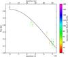 |
Fig. 3 Correlated flux at 10 μm for each of the successful MIDI observations, color-coded following the baseline angle at which the observations were done. The baseline-0 observation (black point) corresponds to the average photometric flux of the observations. The full line shows a fit with the correlated-flux profile of an infinitesimally thin ring of angular diameter θ = 26.3 mas (reduced χ2 = 1.54). |
Figure 3 shows a plot of the correlated flux at 10 μm vs. the uv-distance, showing a uniform decrease in flux up to a baseline length of 52 m, at a level of ~100 mJy. Although it can a priori not be said whether the decrease in flux continues to longer baselines, it is likely that the unsuccessful observations are simply an effect of the correlated flux dropping below the sensitivity limit of MIDI (estimated to be ~80 mJy). Moreover, giving the nearly pole-on orientation of TW Hya, this effect should be symmetric, which is consistent with Fig. 1. Hence, assuming that the unsuccessful observations are intrinsic to the target, we find an upper limit of ~100 mJy for the >50 m correlated fluxes.
To get a first constraint on the scale of the region emitting in the mid-infrared, we add a fit of a simple, infinitesimally thin ring model to Fig. 3. The ring diameter is found to be θ = 26.3 ± 0.3 mas at 10 μm (reduced χ2 = 1.54). At a distance of 51 pc, this corresponds to a ring radius of 0.7 AU, similar to the scale found by Ratzka et al. (2007). Allowing the ring to be inclined, i.e., adding an inclination angle i and a position angle PA as fit parameters, does not lead to a lower reduced χ2 (χ2 = 1.75). In other words, the MIDI observations are fully consistent with a face-on orientation of the disk.
4.2. A scattering component
Both the PIONIER and the NaCo/SAM data indicate that TW Hya is largely unresolved in the near-infrared, with baseline-averaged V2 levels of 0.968 ± 0.005 and 0.949 ± 0.006, respectively (quoted errors are standard errors of mean). Roughly estimating the total flux as composed of a resolved and an unresolved component Fresolved and Funresolved, we have the following relation:  (1)(
(1)( is the visibility amplitude). This shows that the fraction of resolved to unresolved near-infrared radiation is 2−3% (at least, for the spatial ranges probed by the individual observations).
The resolved component in the near-infrared can have two origins: thermal radiation originating from the hot inner-disk regions and/or stellar photons scattered in the disk atmosphere. Unlike thermal near-infrared radiation, which only originates from the hot inner region, scattered light will originate from the global disk. This translates into an immediate drop in visibilities on short baselines.
The azimuthally averaged SAM data clearly exhibit such a drop, revealing that at least a few percent of the L′-band flux is coming from large scales. The typical baselines on which this resolved flux is seen correspond to spacial scales of several tens of AU, confirming that the flux has a non-thermal – thus, scattering – origin.
In the H band, for the more noisy PIONIER data, the origin of the resolved flux is less clear. A useful point of additional information comes from Hubble-imaging by Weinberger et al. (2002). These authors find a ratio of scattered to stellar flux of 0.021 at 1.6 μm. The latter value inferred from large spatial scales (R ≳ 20 AU) is in good agreement with the 2% resolved to unresolved flux ratio determined from the PIONIER data, for smaller scales (≲1 AU). This seems to indicate that the resolved flux in the H-band is predominantly coming from the outer disk regions, and hence has a scattering origin.
The first near-infrared interferometric data of TW Hya were published by Eisner et al. (2006). The wide-band visibility point at 2.14 μm valued V2 = 0.88 ± 0.05, for a 61.7-m baseline. In their modeling, the authors ignore the effect of scattering, and use the observation to constrain the inner-disk characteristics (see Sect. 2). The similar ratio of scattered to stellar flux found at 1.1−1.6 μm (0.024−0.021; Weinberger et al. 2002) and 3.6 μm (0.027; this paper) seems to indicate a roughly constant fraction of scattered flux across the range 1−4 μm. In other words, also in the K-band a contribution of ~2% of scattered light to the total flux can be expected. A later reduction of the Eisner et al. (2006) data point put the visibility to V2 = 0.92 ± 0.05 (Akeson et al. 2011; these authors account for a flux bias). Taking this and Eq. (1) into consideration, the K-band visibility point might not be related to thermal emission, but purely reflect the scattered flux in the K band. Akeson et al. (2011) reach a similar conclusion, where new K-band interferometry confirms an overresolved component.
4.3. Symmetry and variability
As observations tend to be more detailed, protoplanetary disks are revealed to possess more asymmetrical features than originally thought, in some cases very spectacular (e.g., Hashimoto et al. 2011; Grady et al. 2013; Casassus et al. 2013). Also variability is found to be not restricted to the optical and near-infrared spectral range only (e.g., Juhász et al. 2012; Panic et al. 2014). For TW Hya, indications for disk asymmetries and variable disk emission are relatively limited. Roberge et al. (2005) report a sinusoidal dependence in the optical surface brightness on the azimuth angle, and suggest this as an indication for a warped inner disk. In the mid-infrared, Arnold et al. (2012) model speckle-interferometry data with a disk and a hotter-than-equilibrium companion. These authors also indicate variability in the 11.6-μm emission of two epochs. Multi-epoch Spitzer observations might also indicate a variable flux level in the mid-infrared, although pointing errors cannot be excluded for these observations (Najita et al. 2010).
In both our infrared and (sub-)mm data, no significant asymmetries are found. The closure phases in the SAM data were investigated in detail in Evans et al. (2012), but no departures from point symmetry were detected. The deprojected (sub-)mm data show an imaginary component that is effectively zero, also indicating full circular symmetry. Finally, considering the variability, our multi-epoch 50-m baseline observations on MIDI have fully consistent flux levels. Our observations thus do not confirm the variability seen in the mid-infrared based on single-dish observations (at least, within the ~10% calibration accuracy of MIDI).
5. Reimplementing key models
Although we could immediately start modeling the new data sets with a custom radiative transfer code, it is instructive to take an intermediate step. As was mentioned above, several disk models have been published throughout the last decade. Since these models are based on different modeling techniques, it is important to distinguish between the essential characteristics of the models and the model-intrinsic parameters that are less relevant. To achieve this, we make a reimplementation of a selection of models discussed in Sect. 2.
5.1. Three key models
We select three models that were of a key importance for our understanding of the structure of the TW Hya disk. These models are from:
-
Calvet et al. (2002): this is the “gap-discovery” paper, with a detailed argumentation for the dust populations;
Ratzka et al. (2007): this is the first work which argues for a different inner-disk structure, with a smaller inner gap (Rin ~ 0.7 AU rather than 4 AU);
Andrews et al. (2012): this paper presents a direct measurement of the disk size at mm-wavelengths, rather different than the scattered-light edge (Rout ~ 60 AU rather than >200 AU).
We will refer to the three models as the “key” models, and refer to the individual models by the first-author’s name.
Parameters taken for model reimplementation. Essentially all parameter values are exact copies of the original papers.
5.2. The radiative transfer code
Since there have been no indications for strong azimuthal asymmetries in the disk around TW Hya3, it is appropriate to start with an azimuthally symmetric disk model for simulating the data. We will use the Monte Carlo radiative transfer code MCMax (Min et al. 2009) to address the full radiative transfer problem. This code has recently been used to make a coherent picture of several protoplanetary-disk objects (e.g., for HD 100546, Mulders et al. (2011); HD 142527, Verhoeff et al. (2011); HD 169142, Honda et al. (2012)).
In MCMax, an azimuthally symmetric disk structure is set up and, if specified, the code solves for vertical hydrostatic equilibrium by iterating on the temperature and density structures (e.g., Dullemond et al. 2007). A recent update to the code followed on the work of Mulders & Dominik (2012), and implements vertical settling based on the α-disk turbulence prescription. For high turbulence strengths α, grains will experience a strong gas turbulence, and even large grains couple to the gas. Lowering α leads to the decoupling of the larger grains (because of there low surface-to-mass ratios): these grains settle to the midplane.
For all the models, we assume dust particles to be thermally coupled and gas temperatures to be set by the dust temperatures.
5.3. Model reimplementation
We list the disk parameters and a graphical representation of the three key models in Table 2. Each model conceptually has an inner and an outer disk, which implies we could split the table in two. For each model, we carefully reassembled the dust mixtures used in the papers, and traced back the optical constants from the original papers (Fig. 4).
Using a versatile radiative-transfer code, it is possible in principle to fully reconstruct the models with their different particularities. Each of the three models has a different basic model to start from: the Calvet model is based on the D’Alessio et al. (1998) disk model, the Ratzka model uses the disk formalism of Chiang & Goldreich (1997), and the Andrews model makes use of a genuine Monte Carlo radiative transfer code (RadMC, Dullemond & Dominik 2004). The different model structures complicate the model reconstruction in two ways:
-
vertical disk structure: each model has its own formalism for calculating the vertical disk structure (e.g., hydrostatic equilibrium vs. parameterized);
-
disk rim: in each of the three models, the shape of the (inner) rim of the outer disk seems to be an important fine-tuning parameter for getting the right flux in the mid-infrared.
 |
Fig. 4 Comparison of the mass absorption coefficients of the dust mixtures in the different reimplemented models, distinguishing between the inner (dashed) and outer (full) disks. In gray, we show the dust mixture of the final best model (Sect. 6). |
For reference, Table 2 lists to which data the original models were fit. This allows us to interpret the quality of the model reimplementation below in terms of the original model capacities.
 |
Fig. 5 Comparison of the SED data, the MIDI 50-m visibility profile, the deprojected SMA visibilities, and the deprojected VLA visibilities with the reimplemented model data. Along with the fully reimplemented Calvet et al. (2002) model SED, we show the SED consisting of the sum of the contributions of the inner-disk and the outer-disk SED, for which the radiative transfer is done separately. |
5.4. Results
In Fig. 5, the resulting SED of each model reimplementation is shown. Since all three original models reproduce the SED well, any difference between the reimplemented model and the SED is at least partly due to a departure in the intrinsic model structure.
Our reimplementation of the Andrews model accurately reproduces the SED from optical to sub-mm wavelengths. We therefore believe it to be a valid reconstruction of the original model. Like the model reproduction, the original model is constructed with a Monte Carlo radiative transfer code. To imitate the vertical structure, which is parametrized in the original model, we scaled the self-consistent hydrostatic-equilibrium scale height by Ψ = 1.3. At mm-wavelengths, the model flux falls below the observed fluxes. This regime is not constrained by the original model, and possibly reflects the need for an alternative large-grain population (e.g., cm-sized grains).
The reimplementation of the Calvet and the Ratzka models is more problematic. As can be seen in Fig. 5, the former SED has a strong lack of mid- and far-infrared flux, whereas the latter is fitting poorly at (sub-)mm wavelengths. Both models have been produced based on disk-model formalisms preceding state-of-the-art Monte Carlo radiative-transfer modeling. The original models thus lack the self-consistent temperature calculation. In the case of the Calvet model, although the inner disk is relatively tenuous, it is strongly optically thick in the radial direction. The shadowing effects, which could not be taken into account in the original model, cause a strong lack in flux from the mid- to the far-infrared. To demonstrate the effect, we also show the sum of the SEDs made by modeling the radiative transfer of the inner and outer disk separately. The resulting artificial SED clearly reproduces the photometry more accurately, confirming the nature of the original Calvet model. For the Ratzka model, the model reimplementation fits relatively well in the mid-infrared. Here, the inner disk is much more tenuous, and shadowing effects are not playing an important role. The departures of the spectral index at (sub-)mm wavelengths reflects the lack of grains larger than micron-sizes. The latter grains are essential for reproducing the mm-slopes generally seen in protoplanetary-disk SEDs (e.g., Natta et al. 2007). The original model seems not to indicate difficulties in fitting the slope (see Fig. 7 in Ratzka et al. 2007), but our full radiative transfer clearly shows this regime to be problematic. We therefore interpret this departure as a clear indication for a large-grain population.
In Fig. 5, the mid-infrared visibilities on a 50-m baseline are also shown, for each model reproduction (we limit the comparison to the 50-m visibilities for clarity of the plot). Comparing these profiles to the corresponding MIDI data shows that the Ratzka model has the best overall agreement, although a significant departure is seen at wavelengths longer than 10 μm. In both the Calvet and Andrews model, the mid-infrared radiation is coming from a compact inner region: the central part of the optically-thin inner dust region (Rin = 0.02 AU) and the dust ring (R = 0.05−0.25 AU), respectively. In the Ratzka model, the 10-μm feature is associated with the disk rim (Rin = 0.5 AU), and very little mid-infrared emission is coming from within this rim. The original model was fitting the (originally reduced) data relatively well, but the new data reduction has lowered the visibilities at wavelengths above 10 μm. This largely explains the departure.
In the sub-mm regime measured by SMA, the Andrews model is superior, well reproducing the visibility lobes from short to long baselines (Fig. 5). The outer disk in the other two models is much larger (Rout = 140 AU vs. 60 AU for the Andrews model), explaining the steeper drop in visibility amplitude at short baselines. Clearly, the Andrews model was designed to fit the SMA data, and we accurately reimplemented the original model.
Finally, none of the three model reimplementations can reproduce the VLA 9-mm data. For the Ratzka and the Andrews model, the lack of mm-emission (seen in the SED) translates into a visibility level much lower than the one observed. In the Calvet case, we should be more careful in making conclusions. In principle, the original Calvet model should agree to some extent with the mm-visibilities, since this model (in a slightly adapted version) was shown to agree with the original VLA data of TW Hya (see Hughes et al. 2007). However, we already indicated in Sect. 3.4 that the signal-to-noise of those data was much lower than that of the new VLA data presented here. The new data thus put new constraints on the models, which were not available before, and could therefore explain possible departures. However, we believe most of the disagreement between our model reimplementation and the mm-data to be related to the intrinsic model characteristics. Using our full Monte Carlo radiative transfer implementation of the Calvet model, we were unable to obtain similar mm-visibility profiles as the original model. Irrespective of the quality of the previous and the new data, it seems thus impossible to reproduce the bright inner rim in the original semi-analytical model in Hughes et al. (2007).
5.5. Essential features
The results of the model reimplemenation can now be interpreted in terms of a few essential features which need to be investigated in detail.
Different model philosophies.
That different models with strong structural differences reproduce the SED (to some extent) reconfirms that SED modeling is at least partly degenerate. In particular, it does not allow the distinction between two different model “philosophies”: a large-gap disk with a 10-μm excess coming from an optically thin inner region (Calvet and Andrews model), or a small-gap disk with its own silicate feature, with some extra continuum-opacity source inside (Ratzka model).
Grain properties.
Arnold et al. (2012) argue that the differences in mid-infrared opacities of the grain species taken for the Calvet model, on the one hand, and the Ratzka model, on the other, explain why a different hole size (4 AU vs. <1 AU) is found. We question this reasoning because:
-
The differences in the mid-infrared opacities are marginalcompared to the ones at other wavelengths, a wavelength-rangewhich is not considered by Arnoldet al. (2012). Also, the mid-infrared opacities of the Andrews model differ very similarly(like the Ratzka model), yet these authors also have a 4-AU gap.
-
The 10-μm feature in the Ratzka and in the 4-AU gap models do not have the same origin: in the former, radiation is coming from the outer-disk rim, in the latter, from the inner optically thin disk. Therefore, it is incorrect to consider the Ratzka model as a “scaled” 4-AU gap model, i.e., as the same model with a smaller inner hole.
Considering the maximum grain size, the SEDs have shown that large grains are needed to reproduce the mm-slope.
Full radiative transfer.
Our reimplementation of the three models has shown that fully solving the radiative transfer in a disk is important (the same conclusion concerning the inclusion of scattered light is drawn by Pinte et al. 2008a). Structures that are optically thin in the vertical direction are not necessarily optically thin along the radial direction, and can therefore cast a shadow on the outer disk. The loss in intercepted stellar radiation decreases the thermal emission coming from the corresponding scales. This is essentially what was demonstrated for the Calvet model, where the mid-infrared flux to a large extent vanished when self-consistently calculating the model structure.
Solving the full radiative-transfer problem also allows us to use the spectral signature of the small-grain silicates as an important diagnostic for the fit quality. Using simple powerlaw opacity laws (e.g., Eisner et al. 2006; Akeson et al. 2011) to some extent misses the interpretation in terms of realistic particle characteristics (e.g., composition, grain sizes).
To 4 AU or not to 4 AU?
Perhaps the most interesting parameter for the TW Hya disk is the size (or size range) of the inner gap. As we have shown, the current 4-AU gap models do not manage to model the MIDI visibilities, and also the new VLA data seem not to confirm the essential visibility null found in the previous VLA data. However, the data presented in Arnold et al. (2012) still are in agreement with a 4-AU inner gap, so some structure change on this scale still might be needed for explaining all data.
6. Radiative transfer modeling
The inability of the previous models to fully explain the combined data set confirms the need for the development of a new disk model. This is what is done in the current section.
6.1. Model fitting strategy: a genetic algorithm
We decided to use a genetic fitting algorithm for the radiative transfer modeling of the spectrally and spatially resolved data. This fitting strategy allows for an efficient exploration of the parameter space and thereby limits the risk of getting stuck in local χ2-minima.
The genetic-algorithm formalism used for the model fitting in this work is described in Appendix A.
 |
Fig. 6 Model refinement strategy: we start with a simple disk with a vertical inner rim (left), we then introduce a rounded inner rim (middle), and finally also concentrate the largest grains towards the inner disk regions (right). |
6.2. Stellar properties and dust composition
In principle, the complete set of parameters involved in a disk model could be included into the fitting process. However, even using a dedicated fitting strategy, we have a strong interest to minimize the actual fitting parameters, speeding up and mitigating the fitting process.
During the radiative-transfer modeling, the stellar properties are kept fixed to literature values: stellar mass M⋆ = 0.6 M⊙, luminosity L = 0.25 L⊙, effective temperature Teff = 4000 K, distance d = 51 pc (references in Ratzka et al. (2007); the luminosity was slightly increased). We also fix the disk inclination to i = 0°: we model the deprojected visibility curves in the (sub-)mm, and the relatively poor uv-coverage and/or the error level of our infrared interferometry makes the 6-degree inclination correction irrelevant.
For the dust composition we use a mixture of amorphous silicates (Table 3) and carbonaceous grains. Opacities are calculated using a distribution of hollow spheres (DHS; Min et al. 2005) for the particle shapes. To model the silicate composition, we use the diagnostics of the 10-μm feature in a Spitzer IRS spectrum of TW Hya (kindly provided by T. Ratzka; see Ratzka et al. 2007), using a procedure similar to the one in, e.g., van Boekel et al. (2005) and Juhász et al. (2010). The contribution of the dust to the spectrum is fit using the following equation:  (2)where κν,i is the dust opacity of silicate species i, and Ax are the weighting factors of the individual terms. In words, we assume the dust emission to be composed of the thermal (continuum) emission of two black-body components (Bν) at characteristic temperatures Twarm and Tcold, and optically thin emission of the dust grains at a characteristic dust temperature Tdust.
Amorphous silicates used for the spectral fit.
The best fit to the Spitzer spectrum is reached for a mixture of pure amorphous magnesium-iron olivines (MgFeSiO4). Our final dust mixture is taken to be 80% of these silicates and 20% of carbonaceous grains (Preibisch et al. 1993), the latter representing the continuum opacity. A constant dust-to-gas ratio of 0.01 is assumed. Following our Spitzer-spectrum fit, we also fix the index of the particle size distribution to −3.5 (Mathis et al. 1977) and the minimum particle size to amin = 0.01 μm (however, the maximum grain size amax will be varied; see Sect. 6.4).
6.3. Data selection
Rather than picking all data to do the fit, we restrict ourselves to a subset for the model runs. As indicated in Sect. 4, the near-infrared data (PIONIER + NaCo/SAM) are dominated by an overresolved scattering component. The structural information in the data is therefore limited. As we will show below in Sect. 8, the model visibilities are strongly dominated by our assumptions on scattering (isotropic vs. anisotropic). Immediately including the near-infrared data would therefore complicate our focus on the disk structure by having to address simultaneously this scattering problem. We hence only include the high angular resolution data that are dominated by thermal radiation of the disk, i.e., from the mid-infrared to mm-wavelengths.
Concerning the MIDI data, we averaged the 25-m baseline and the 50-m baseline observations to two correlated flux profiles at an averaged baseline of 26 m and 48 m. Also the photometric data were averaged to a single total spectrum (photometric data of 2011 were ruled out in the average due to poor quality).
Finally, for the SED data, we exclude the VLA 4-cm and 6-cm detections. The photometric points at these wavelengths might be affected by free-free emission, something that will be addressed in Sect. 7.6.
The total χ2 associated with the fit is then:  (3)where the MIDI-parts of the χ2 refer to the total spectrum (00 m), averaged 25-m correlated fluxes, and averaged 50-m correlated fluxes.
Below, we describe the process that leads to our final disk model; a graphical representation of the model refinement strategy is shown in Fig. 6.
 |
Fig. 7 Plots of the best models corresponding to a simple disk (red, dotted), a simple disk with a rounded rim (blue, dashed), and a simple disk with a rounded rim and a centrally-concentrated large grain population (green, full). |
Parameter ranges for disk models.
Parameter values and estimated uncertainties for the best fit of the different models.
6.4. Simple-disk model
Starting our modeling work from first principles, we begin with a simple radially homogeneous disk model with a vertical inner rim. This model has six free parameters: inner radius Rin, outer radius Rout, dust mass Mdust, surface-density power p (i.e., Σ(R) ∝ R− p), maximum grain size amax, and the turbulence mixing strength α. The latter number parametrizes the settling of the dust: the weaker the turbulence, i.e., the lower α, the stronger the settling of large grains. Since the settling is grain-size dependent, we split the grain population in logarithmic size bins4. The parameter ranges that were tested in the modeling run are shown in Table 4. We note that the ranges cover the physically realistic/interesting values for the specific parameters (e.g., testing Rin> 1 AU is unnecessary, since this would not produce enough flux for simulating the 10-μm feature).
 |
Fig. 8 Convergence plots for Rin (top) and the surface density power p (bottom), for the simple-disk model. The titles of the individual plots indicate to which data set the shown χ2 values correspond (e.g., for MIDI: |
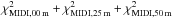
Figure 7 shows the model resulting from calculating 20 generations of 200 models, and the corresponding parameter values are included in Table 5. The fit reaches a reasonable quality for the SED and the SMA data, and the model also reproduces the global flux levels of the MIDI data. However, the visibility profile at VLA wavelengths clearly differs from the actual data (for the non-trivial part of the data): at short baselines, the model shows the oscillatory behavior associated with a sharp disk rim (cf. the SMA data), whereas the VLA data have a much smoother profile. Nevertheless, the found parameters are interesting, in the sense that they confirm the presence of large grains (amax ≥ 1 mm), a Ratzka-model scale for the inner rim (~ 0.7 AU), and an Andrews-model scale for the outer-disk edge (~ 60 AU).
Table 5 contains an estimate of the uncertainty on the different parameters (see Sect. 7.1 and Appendix B). An instructive way to visualize the significance of the different parameters is to make a plot of the χ2-values of the calculated models vs. the parameter values corresponding to these models. Using different colors, we can distinguish between the different generations to which the models belong. Going from the first to the last generations, one expects to see a transition from randomly distributed parameter values towards a more concentrated neighborhood, the absolute minimum in the χ2-space. The plots could therefore be called convergence plots, showing the gradual convergence for the different parameters. For unconstrained or degenerate parameters, on the other hand, this behavior will not be seen: other constraints are then needed.
In Fig. 8 we show two different examples of these convergence plots, for Rin and p. The plots show both the total χ2-values and the χ2-values of the individual data sets (cf. Eq. (3)). As can be seen in the upper plots, the convergence of Rin is almost completely determined by the MIDI data, whereas the other data show a more random-like distribution in χ2-values for different values of Rin5. In the second case, for the surface density power p, a rather different behavior is seen. Clearly, the lowest χ2-values are reached for the lowest p-values, as far as the MIDI and the SED data are concerned. By contrast, much lower χ2-values for the VLA data are reached if larger values (p> 1) are taken. For the current modeling run, the convergence seems thus to be dominated by the MIDI and SED data, which outweighs the fit to the VLA data.
6.5. Simple disk with a rounded inner rim
The MIDI fluxes are mainly determined by the thermal emission of small dust grains at relatively warm temperatures (≳100 K), thus relatively close to the central star (and close to the disk surface). The convergence to a low value for p in the simple-disk model, dominated by the MIDI data (Fig. 8), could therefore point to a different density regime in the inner regions of the disk, rather than being representative for the complete disk. Verifying models with steeper surface densities (e.g., p ≳ 1) indicates that the inner region of the disks are optically thick in the radial direction up to high scale heights. As a consequence, the sharp, vertical rim strongly intercepts stellar radiation and reradiates it mainly in the radial direction (i.e., not in the direction perpendicular to the disk, where the observer is situated). In the low-density case, the radial optical depth at small radii is much smaller, and a significant disk atmosphere is reachable for thermal re-emission along the vertical direction.
As an alternative to a vertical wall, we can introduce a rounded-off wall. The smoother transition from the inner hole to the “full” disk avoids the strong geometric effects due to observing the disk pole-on. More into detail, the parametrization of a smooth wall also extends the possibilities for the fitting algorithm to reproduce the MIDI correlated fluxes, and decreases the possible biasing of the fit of the other datasets.
We utilize the rim structure used in Mulders et al. (2013b) to model the disk rim of the Herbig Ae/Be star HD 100546:  (4)Here, here Σexp is the surface density at the radius Rexp where the drop in surface density starts, and w is a dimensionless rim width. In other words, we assume that at a certain transition radius, the surface density decreases exponentially towards the inner disk rim. The rim shape has a direct link to hydrodynamical simulations of a transition disk in the presence of a (sub-)stellar companion, to which we go deeper into in Sect. 7.3. The modification thus introduces two new free parameters: Rexp and w; see Table 46. For simplicity we keep amax fixed to 1 cm, the value found before.
Figure 7 shows the resulting best fit after calculating 30 generations of 200 models. A more accurate fit is reached for the MIDI data, and the total χ2-value lowers from χ2 = 94.2 to χ2 = 67.1. Yet, some clear difference between the model and the actual data are apparent. As far as the spectrally resolved data are concerned (SED, MIDI), these differences are not necessarily problematic: at least part of the model deviation can be related to the exact dust composition, which is not included in the parameter fitting here and therefore cannot be expected to agree perfectly. However, for the monochromatic visibility data, departures in shape will be mostly related to the exact model for the dust distribution. In the case of the SMA data, a clear departure in shape is seen for projected baselines above 200 kλ. For the VLA data, the departure is even more problematic: as in the simple-disk case, the model has a completely different profile at short baselines.
6.6. Intermezzo: sub-mm vs. mm-visibilities
The current model geometry has difficulties in simultaneously accommodating the sub-mm and the mm-data. The convergence to the final model is currently mainly determined by the mutual weight of the individual data sets, and clearly the SMA data have more weight in the fit than the VLA data.
The visibility profiles of the SMA and VLA data in Fig. 7 indicate that the disk looks very different in the two wavelength regimes. Since the disk is optically thin at both wavelengths, the dominant opacity sources must be distributed in a different way throughout the disk (i.e., the difference in visibilities is not an optical-depth effect). The steep visibility decrease at sub-mm wavelengths with respect to the smooth decrease at mm-wavelengths is evidence of a more compact distribution of the region emitting in the millimeter. Also, the visibility oscillations in the SMA data are not apparent in the VLA data, indicating that we do not have sharp edges within the spatial resolution range of the VLA observations (at least, at the mm-wavelengths).
One way to make a smoothly decreasing visibility profile with centrally concentrated emission is to make a centrally concentrated dust distribution that rapidly decreases outwards. Since the surface density is steeply decreasing with radius, the outer edge of the disk will not be in high contrast with the region devoid of dust, avoiding the strong oscillatory behavior (“ringing”) in the visibility curve. However, the above distribution should only concern the mm-emission from the dust: for the sub-mm data, we will still need a dust distribution with a sharp outer edge.
6.7. Compact distribution of the largest grains
From our above reasoning, it seems essential to distinguish between two dust populations: one determining the disk at sub-mm wavelengths vs. one that sets the brightness distribution at mm-wavelengths. For the implementation of the dust settling, we have split up the full grain distribution in bins of an order of magnitude in grain size (0.01−0.1 μm, 0.1−1.0 μm, etc.; see Sect. 6.4). We show a plot of the opacity curves κλ of each of the size bins in Fig. 9. It is clear that the grain size ~ 100 μm determines a transition between size bins that have κSMA ≫ κVLA and κSMA ~ κVLA. Therefore, most of the disk appearance at sub-mm wavelengths will be determined by the sub-100-μm dust. This allows us to deliberate our large-grain population, and freely distribute it throughout the disk, without considerably disturbing the visibilities at sub-mm wavelengths.
We propose to implement the redistribution of the >100-μm dust by introducing a new parameter, the surface density power p> 100 μm for these large grains. We assume the same surface-density profile as in Eq. (4) for these large grains, only with a different power p> 100 μm (i.e., p> 100 μm ≠ p).
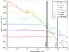 |
Fig. 9 Mass absorption coefficients per order of magnitude in grain size, for an n(a) ∝ a-3.5 size distribution (within each bin). The vertical lines indicate the wavelengths of the SMA and VLA observations, allowing the comparison of the relative opacity contribution for each of the grain size bins. |
The final model run deserves the following comments:
-
The above models clearly showed the SMA fit to outweigh the fit of the VLA data. This is an intrinsic issue due to the relative level of accuracy of the former data set with respect to the latter. In order not to favor one data set over the other, we readjust the relative weights of the two data sets by decreasing and increasing them by a factor of 2, respectively (i.e.,
 ;
;  ). Inspection of the fits a posteriori shows that this factor leads to a satisfactory reproduction of all data sets (at least by eye).
 We found it necessary to fix two parameters to get a valid fit. First, we fixed amax to 1 mm. As can be inferred from the previous model fits (the shown models in Fig. 7), the VLA-visibilities at short baselines are overpredicted for amax = 1 cm. Taking amax = 1 mm lowers the mm-flux, which allows the model to reach valid visibility levels. The second parameter we fix is the settling parameter α. The strongest diagnostic for α in our data set is the SED shape in the range λ = 100 − 500 μm: this wavelength range corresponds to the thermal emission of the outer flaring disk, and it is exactly α which determines the amount of flaring in the different dust populations. However, test model runs show that subtle effects at longer wavelengths (with now two equally contributing visibility data sets) outweigh the determination of α from the few SED points in the range λ = 100 − 500 μm. We therefore fix α = 10-5, the relatively well constrained value found before.
We limit the model fitting algorithm to a compact parameter space around the best parameters of the previous models. The only parameters we give a large freedom are the surface density powers p and p> 100 μm, and the dust masses Mdust,< 100 μm and Mdust,> 100 μm. We note that we indeed split up the dust masses in the small and large grains, since the different spatial distribution for the two grains populations does not necessarily mean that their relative abundance should be the same as for a radially homogeneous disk.
7. Discussion
7.1. Parameter validity range
The outcome of a modeling run is a set of parameters, corresponding to the best-fitting model. Getting an idea on how well the model fits the data, i.e., determining the uncertainty on the determined parameters, is a non-trivial problem.
Different techniques exist for determining the validity range of fit parameters (see, e.g., Andrae 2010 for a concise overview). Several of the techniques are based on a relatively extended sampling of the parameter space (e.g., Markov Chain Monte Carlo methods, parameter grid methods), or make use of refitting the slightly modified data set (e.g., resampling, bootstrapping techniques). In the case of highly dimensional parameter spaces, with computationally expensive model calculations, most of the techniques become highly demanding in terms of computation time/power.
The reason for using a genetic fitting algorithm for our modeling work was exactly to limit the computational effort needed. We therefore also have interest in finding a method that gives error estimates in a reasonably simple way. Several methods have been used to find validity ranges for parameters when using a genetic algorithm for fitting. Cantó et al. (2009) use a data-resampling technique for generating artificial data sets, which are then refitted. De Geyter et al. (2013) also make use of additional fits, but each time on the same data set (here, the uncertainty is reduced to the reproducibility of the best model)7. For both methods, new fits are thus required, multiplying the computation time by the number of redone fits. A different approach is to specify an ad hoc parameter Δχ2, defining a range of calculated models and hence parameters that are still “valid” (Johnston et al. 2011).
We make use of a method based on the collection of models that is calculated to get to the best model. The method is explained in Appendix B. In essence, the parameters of the calculated models are resampled on a regular grid, which allows us to use a Bayesian inference method as in, e.g., Pinte et al. (2008b) or Lebreton et al. (2012).
7.2. Parameter values of different models
Table 5 allows us to compare the values of the parameters shared by the subsequent model geometries, and compare with previously proposed disk models.
The simple-disk model with a vertical rim has an inner-disk geometry that is well constrained, with an inner radius of 0.7 AU. The scale is exactly what was found by Ratzka et al. (2007), and also confirms our simple-ring fit in Sect. 4.1. Our radiative transfer modeling shows that a vertical rim is not properly explaining the full 10-μm emission profile in the MIDI correlated fluxes, something that is improved upon by introducing a dust-depleted inner region (i.e., the rounded rim). This moves in the inner radius to a less constrained value of 0.3−0.5 AU. The starting point of the “rounding-off” of the inner rim lies around ~3 AU, as can be inferred from both model geometries that include the rounded rim. We note that Rexp does not correspond to the radius of the maximum surface density. The latter lies closer to the central star, roughly around 2.5 AU for the disk models with Rexp ~ 3 AU. The resulting surface-density profile, which is then smoothly decreasing inwards of this radius, is thus rather different than the profile with a sharp transition at 4 AU, typically used to model the disk (e.g., Thi et al. 2010; Andrews et al. 2012; Arnold et al. 2012; Zhang et al. 2013).
For Rout, we find relatively well constrained values around 60 AU for the three tested model geometries. These values confirm the value of 60 AU found by Andrews et al. (2012). As was already mentioned by these authors, the value differs from the outer radius of the disk as detected in scattered light and CO (>200 AU). We go deeper into this difference in Sect. 8.2, where we also describe the constraints coming from our near-infrared data.
A final parameter we consider here is the total dust mass Mdust. For the first two model geometries, we find a dust mass around 2 × 10⁻⁴M⊙; for the final geometry, the total dust mass is around 1 × 10⁻⁴M⊙. The difference between the two is due to the maximum grain size amax in the models (1 cm vs. 1 mm): the higher amax, the lower the mass-averaged absorption coefficients (since small grains dominate the absorption/emission at short wavelengths). Comparing the mass of our disk model with the masses of the reimplemented models in Sect. 5 shows that our estimate is relatively low. The difference in mass estimates is strongly related to the different opacities assumed in the different models (Fig. 4). Since the disk is optically thin at long wavelengths, the emission at long wavelengths is proportional to the mass and the opacity at these wavelengths. For a given millimeter flux, a higher assumed opacity will therefore lead to a lower dust mass. This is exactly what we see here: our model has high dust opacities at millimeter wavelengths, and this results in a relatively low dust mass. Any comparison of model dust masses therefore translates into the inherent uncertainties on dust properties.
A graphical representation of our newly proposed disk model is shown in Fig. 10.
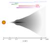 |
Fig. 10 Current image of the TW Hya transition disk. In black, we represent the centrally concentrated large-grain population, which is also strongly vertically settled. The light-gray outer-disk region between 60 AU and >200 AU is not constrained by our radiative transfer model, but is discussed in Sect. 8.2. We also indicate the regions constrained by the different data sets. The near-infrared data provide only weak constraints (see Sect. 8). |
7.3. Rim shape
Studying the geometry of the inner region of protoplanetary disks is challenging, in particular concerning the shape of the inner disk rim (Dullemond & Monnier 2010). Initial radiative-transfer models with vertical inner rims have near- and mid-infrared excesses that are strongly inclination dependent (Dullemond et al. 2001). Later models for the inner rim self-consistently led to a rounded rim structure, a consequence of the temperature dependence of dust condensation on gas density (Isella & Natta 2005).
In the case of transition disks, the radius of the disk rim is (much) larger than the typical condensation radius of the dust grains and is hence not determined by the condensation temperature of dust. A possible hypothesis is that the inner rim of the transition disk is shaped by the presence of a (sub-)stellar companion inside the gap. Recently, Mulders et al. (2013b) made a detailed study of MIDI observations of the (pre-)transition disk object HD 100546. They showed that the observations agree with a disk with the surface-density profile in Eq. (4). Hydrodynamical simulations of the inner disk region then show that the surface density can be reproduced by assuming a ~60 MJ companion within the disk gap.
Our correlated-flux profiles do not contain the clear diagnostics as present in the HD 100546 data in Mulders et al. (2013b), but we do show that the smooth surface-density profile leads to a better reproduction of the correlated fluxes than assuming a sharp transition. This indicates that a companion might have shaped this inner rim. Properties of a possible companion could be derived using similar hydrodynamical simulations of the inner-disk region, something that is beyond the scope of this work. A planetary body within the central ~0.1 AU could agree with the proposed companion to TW Hya at 0.04 AU (Setiawan et al. 2008), which existence is yet under debate (Huélamo et al. 2008).
Although a companion hypothesis is attractive, other processes might contribute to (or even dominate) the creation of the inner cavity. There is strong evidence that photoevaporation plays an important role in the dispersal of the inner disk of TW Hya (Pascucci et al. 2011). Moreover, Baruteau et al. (2013) make clear that the gaps carved out in disks by companions of a Jupiter mass or less will be narrow annuli, and not cavity-like. Full dynamical simulations of the inner disk region, taking previous results on photoevaporation and our constraints on the dust into account, will be an important next step.
7.4. A compact distribution in the largest grains
Figure 7 showed that the visibility profiles at sub-mm and mm-wavelengths differ significantly. Differences in visibility profiles at different mm-wavelengths are seen for other T Tauri stars, and led to a common approach of modeling the data at different wavelengths separately (e.g., Isella et al. 2010). The differences in derived surface-density profiles can be interpreted in terms of a radially varying β, the opacity slope at millimeter wavelengths (κλ ∝ λ− β). This change in millimeter opacities is then seen as evidence that grain sizes are decreasing with distance from the central star (Guilloteau et al. 2011; Pérez et al. 2012), a conclusion that is also reached for younger (Class 0) objects (Kwon et al. 2009).
The aim of this work is to find a radiative transfer model that directly incorporates the dust emission at different wavelengths. Making models with a radially homogeneous grain composition, i.e., with the same relative abundances for the grain-size bins throughout the disk, clearly showed to be unsuccessful. Instead, the visibility profiles inspired us to propose to decouple the largest grains from the smaller-grain population. This, in turn, resulted in a model with two different surface density regimes. For the grains with sizes below 100 μm, the expectation value for the surface-density power is p = 0.6 ± 0.2 (the best-fit model has p = 0.5). This is close to the value 0.75 found for the Andrews model, see Table 2, based on the same SMA data set. For the larger grains (a> 100 μm), the surface density power in the best model is two times higher.
The spatial and size distribution of dust grains in protoplanetary disks is determined by the processes of dust growth, fragmentation, and transport in viscously evolving gas disks. Birnstiel et al. (2012) present a simple model for the dust evolution in disks that agrees with high-level simulations of the incorporated processes (Birnstiel et al. 2010). Two limiting cases are determined: the fragmentation-limited distribution, where the dust particles are in a steady state in which coagulation and fragmentation balance, and the drift-dominated distribution, where dust particles are drifting away more rapidly than being replenished by growth. The dominant regime in a certain part of the disk depends on parameters like the turbulence level, the velocity at which grains fragment, and the initial gas-to-dust ratio.
Birnstiel et al. (2012) show that the drift-dominated disks have a dust surface density proportional to R-0.75, for gas-disk profiles with Σgas ∝ R-1, and point out that the Andrews model agrees with this surface-density profile. As was already indicated, our surface density for the <100-μm grains agrees with this profile, except that our assumption of a constant dust-to-gas ratio leads to a gas surface density of the form  (5)where A and B are constants. However, the sum of the shallow and the steep density profile leads to a surface density that differs by less then 10% from a “regular” R-1 profile, for almost the complete disk. This implies that the approximation for this simple drift-dominated disk model is valid. Concerning now the grain population larger that 100 μm, we have a surface-density profile that is considerably different from the drift-dominated case. Interestingly, the found expectation value p> 100 μm = 1.4 ± 0.2 (and p> 100 μm = 1.3 for the best-fitting model) is very close to surface-density power 1.5 corresponding to the fragmentation-dominated distribution (Birnstiel et al. 2012). It seems therefore that the different traced surface densities can be related to physically different regimes within the disk.
For typical simulation results in Birnstiel et al. (2012), disks with an age of a few Myr have maximum particle sizes that are drift-dominated in the outer regions and fragmentation-dominated in the inner regions. In addition, the models also show that the largest grains are found in the inner region of the disk. The results we get from our radiative-transfer modeling seem to confirm this picture. For the largest grains, thus probing the inner disk region, we indeed find a surface density that has a fragmentation-dominated character; for the smaller grains, probing also further-out regions in the disk, we seem to confirm a drift-dominated surface density.
7.5. Linking the dust emission to gas properties
Our analysis has implicitly substituted “modeling the disk structure” by “modeling the dust distribution”. The contribution of the gas to the disk structure is only incorporated in terms of the vertical hydrostatic equilibrium and the vertical settling of the dust grains. In order to investigate the gas and dust distribution simultaneously, gas-emission diagnostics would be required, preferably spatially resolved (see, e.g., Andrews et al. 2012 for the analysis of the outer disk in CO). Still, a few indirect links can be exploited to couple the disk model to the intrinsic gas properties.
By its nature, the turbulent mixing strength parameter α couples the gaseous structure of the disk to the dust distribution. Mulders & Dominik (2012) model median SEDs of Herbig stars, T Tauri stars, and brown dwarfs, and find α = 10-4 to be a representative value across this range of stellar masses (their analysis is based on the same radiative-transfer code as the one used here). The here inferred value of α ~ 10-5 seems to indicate that TW Hya has a more-settled disk than average. Hughes et al. (2011) model the spatially resolved CO mm-emission of TW Hya, and estimate that α ~ 10-3 − 10-2, in line with accretion-based estimates of α for other protoplanetary disks (α ~ 10-2: Hartmann et al. 1998). The gas-based (i.e., CO emission, accretion) estimates of α clearly indicate a higher value than the α-value found here. Although more work on reconciling the two approaches is needed, this apparent inconsistency might simply indicate that the assumption of a single, constant α throughout the disk is most likely invalid (see, e.g., dead zones). Therefore, different estimates might be dominated by specific disk regions, which does not necessarily gives the same values.
A second diagnostic for the gas is offered by the temperature structure of the disk, a direct output of the radiative-transfer model. ALMA observations of TW Hya have recently led to the discovery of the CO ice line at ~ 29 AU, by inferring the inner-edge location of N2H+ in the midplane (Qi et al. 2013). These observations provide an independent measure for the midplane temperature. Our radiative transfer model has a midplane temperature of 14 K at 29 AU. This value is reasonably close to the temperature of ~17 K inferred for the N2H+ inner-edge location, agreeing with expected CO sublimation temperatures (Qi et al. 2013). This indicates that our purely dust-based model leads to a temperature structure that might be in reasonable agreement with the temperature structures inferred using gas-diagnostics, at least for regions where gas and dust temperature are similar.
7.6. Contribution of excess radio continuum emission
The data analysis presented here is restricted to λ< 1 cm, since emission at cm-wavelengths is possibly affected by the presence of an ionized wind (Sect. 3.5). Here, we shortly discuss the nature of the radio continuum excess, and justify our model assumption of pure dust emission at sub-cm wavelengths, in particular for the resolved 9-mm VLA data.
Pascucci et al. (2012) analyze the contribution of free-free emission in the long-wavelength SED of TW Hya. They conclude that the 7-mm emission agrees with pure dust emission, whereas the 3.5-cm emission (Wilner et al. 2005) clearly shows an excess. The new 4.1-cm and 6.3-cm VLA detections of TW Hya allow us to repeat the Pascucci et al. (2012) analysis, and fit the actual contribution of the cm-excess8. Following their approach and other arguments, the following conclusions can be made on the long-wavelength SED of TW Hya (Appendix C):
-
the contribution of a radio excess at λ = 9 mm (i.e., the wavelength of the modeled VLA observations) is low, perhaps on the level of 5%;
-
the potential radio-excess source cannot be point-like;
-
even at wavelengths as long as 4 cm, the dust emission seems to be detected, confirming the earlier suggestion by Wilner et al. (2005) that for TW Hya, dust emission is important even at wavelengths of 3.5 cm.
The non-point-like nature of the excess implies that any attempt to model this excess would require including a parametrized geometry of the responsible region. This is a non-trivial issue, and the data quality is likely not good enough to assess this problem. Taking the uncertainty level of the data and the arguably small excess contribution into account, we can therefore justify our modeling assumption of pure dust emission at 9 mm, i.e., the use of a pure radiative-transfer model.
 |
Fig. 11 PIONIER and NaCo/SAM (squared) visibilities with the predicted visibilities for the final best model (full line), under the approximation of isotropic scattering (red) and full scattering (green; i.e., also including non-isotropic scattering). The dotted green line shows the predictions for the same model, but this time with large grains in the disk atmosphere (simulated by increasing the turbulence strength α from 10-5 to 10-3). Finally, the dashed line again shows the predicted model visibilities of the best model, but now with an outer radius of 200 AU for the < 10-μm sized grains. |
8. Near-infrared analysis
For reasons given in Sect. 6.3, we have excluded the near-infrared data from the radiative-transfer analysis up to this moment. We now investigate how these data and other scattered-light observations can be accommodated within our best model.
8.1. VLTI/PIONIER and VLT/NaCo data
In Fig. 11, we plot the (squared) visibility vs. baseline corresponding to the VLTI/PIONIER and NaCo/SAM observations. Directly calculating the visibilities at λ = 1.65 μm (PIONIER) and λ = 3.6 μm (NaCo/SAM) for the final best model in Sect. 6 gives the result shown in red. Although the model curves qualitatively reproduce the trend in the data, the model underestimates or overestimates the global visibility level of the PIONIER or NaCo/SAM data, respectively.
All radiative-transfer simulations made up to this moment were based on an isotropic treatment of the radiation field. Given the importance of scattered light in interpreting the near-infrared data (see Sect. 4.2), we now recalculate the same model based on full (anisotropic) radiative transfer. A correct treatment of scattering, indeed an intrinsically anisotropic process, leads to visibilities that are clearly significantly higher than the visibilities calculated under isotropic scattering (Fig. 11). This increase in disk-star contrast9 is a consequence of the forward scattering in combination with the pole-on orientation of the TW Hya disk. Indeed, grains in the disk atmosphere will tend to scatter the stellar radiation in the radial rather than the perpendicular (i.e., the observer’s) direction, making the disk fainter (see also Mulders et al. 2013a).
Taking anisotropic scattering into account improves the agreement of the model with the PIONIER data10. For the NaCo/SAM data, also the full-scattering model fails to reproduce the visibilities. The latter might point to the need for grains with different scattering properties.
To further investigate this, we recalculate the visibilities for an increased amount of large grains in the disk atmosphere. Instead of adding other grains to the model, we artificially stir-up large grains by increasing the turbulent mixing strength (from α = 10-5 to 10-3). As shown in the right panel of Fig. 11, this leads to a much better reproduction of the SAM data, a consequence of the higher scatter efficiency of the larger grains (resulting in a lower star–disk contrast). Of course, a real increase in turbulence is excluded by the fit of the other data (since this completely changes the vertical distribution in all grain populations), and also the reproduction of the PIONIER data is affected. Yet, this test shows that adding a small, separate population of micron-sized grains to the upper atmosphere might allow us to fully incorporate the SAM observations. Particles like this could remain high up in the atmosphere when they are fluffy (like “snowflakes”), i.e., when they have large surface-to-mass ratios and hence a strong coupling to the gas (Mulders et al. 2013a).
8.2. Outer radius in scattered light
The outer radius of the disk (Rout) is consistently found to be ~ 60 AU. This value is clearly smaller than the outer detection radius of the disk in scattered light, which is at least 280 AU (Roberge et al. 2005). However, convergence plots of Rout indicate that the parameter is mainly constrained by the SMA data, i.e., by the emission of large grains. For the small grains, which will dominate the scattering since they are dominating the disk atmosphere (due to settling), we do not have any strong constraints on Rout in our data.
Andrews et al. (2012) already indicated that the outer radius of the disk in large grains is much smaller than it appears in gas emission (as traced by CO). In the current scenario, the small grains seem thus well coupled to the gas, and span a region up to at least 200 AU in radius, whereas the large grains are found only up to 60 AU. As a test, we can therefore add small grains to the region outside 60 AU, hereby effectively introducing a decoupled Rout for the small grains. In principle, this should not influence the model fit to the thermal emission data.
To the plots in Fig. 11, we added the corresponding model plots where we let the surface density of the grains smaller than 10 μm continue up to 200 AU. The changes to the model curves are low, and clearly such a change is not detectable with our near-infrared data sets. Making corresponding images shows that, at least qualitatively, we can get synthetic near-infrared images with large outer radii, but for which the fit of the here-presented data set (near-infrared to cm interferometry) is not changed.
Recently, Debes et al. (2013) investigated the depression in the surface brightness of the disk at R ~ 80 AU, already reported in Krist et al. (2000). The depression is interpreted as a (partially filled) gap in the disk. Since the detection is based on the scattered light of the disk, we lack any strong diagnostics to reconfirm this gap. Our disk model also does not require any material to be located that far from the central star, i.e., we currently cannot confirm if a gap would be present in the thermal dust emission.
9. Summary and conclusions
Although the transition disk around TW Hya has been studied in detail, the variety of disk models in the literature indicates that the disk structure is still under discussion. Combining high-angular-resolution data that span five orders of magnitude in wavelength, our aim was to develop a radiative-transfer model that fully incorporates the dust distribution around the star, with a focus on the inner-disk region. This work has led to the following conclusions:
-
1.
Reimplementing existing radiative-transfer models for the TW Hya disk shows that the published models can indeed explain part of the combined data set, but fail to reproduce data at other wavelengths. This shows that a multiwavelength analysis is essential to fully characterize the disk. Also, this exercise already points to some model properties: the need for large (≫μm) dust grains, the importance of full radiative transfer for explaining the disk, and the fact that the new mm-interferometry gives completely new constraints on the disk structure.
-
2.
A simple disk structure with a vertical inner rim and a radially homogeneous composition (from small to large grains) cannot properly explain the data. From the MIDI data, we infer an inner region with a lower surface density.
-
3.
As a first modification to the simple disk model, we introduce a rounded rim by exponentially reducing the surface density (with respect to a standard power law surface density) inwards of a specified radius. Mulders et al. (2013b) have shown that this rim profile follows from hydrodynamical simulations of a low-mass companion opening a disk gap. Our MIDI data agree with the expected mid-infrared emission of such a rim. Although linking the gap in the TW Hya disk with the presence of a companion is tentative, other mechanisms might lead to similar rim geometries.
-
4.
The mm-emission as observed with VLA originates from a spatially more compact region than the sub-mm emission observed with SMA. We interpret this as evidence for a more compact distribution of the largest dust grains, something that is also seen in other disks (e.g., Pérez et al. 2012). We model the >100-μm grains with the same surface density profile as the smaller grains, but with a steeper surface density power. This allows us to reproduce both the SMA- and VLA-visibilities, to a reasonable extent. We note that for TW Hya, the VLA data allow us to trace the imprint of dust emission to wavelengths as long as 4 cm, in line with earlier suggestions by Wilner et al. (2005).
-
5.
Our final disk model (Fig. 10) has an inner radius of 0.3−0.5 AU, an outer radius of ~ 60 AU, and a maximum in the surface density around 2.5 AU, where the surface density smoothly decreases inwards.
-
6.
For the radiative-transfer analysis, we do not focus on the near-infrared data, since these depend predominantly on the scattering properties of the dust. Instead, we compare the visibilities predicted by the best-fit model with the actual data. This comparison shows the importance of taking the full scattering properties of the dust into account. The predicted visibilities reproduce the H band data reasonably well; for the L′ band data, a small population of possibly fluffy grains might be needed in the disk atmosphere for predicting the correct visibilities. A population of small grains at large distances from the star, as observed in scattered light images, can easily be incorporated in the final disk model.
An inner disk edge that is larger than the dust sublimation radius was already used in a disk model in Trilling et al. (2001), although not interpreted as a departure from a classical disk structure.
The hint for asymmetry in Arnold et al. (2012) is interpreted as an indication for a (unconfirmed) secondary source, and not as an indication for disk asymmetries.
We refer to Mulders & Dominik (2012) for more details on the α parameter and its implementation in MCMax.
It might seem that the SMA data also help to constrain the fit. However, the convergence here is only apparent: essentially all models in the SMA plot belong to later model generations (green to violet color), where Rin is already well-constrained (by the MIDI data). The SMA data thus do not help constraining Rin.
The analysis of Pascucci et al. (2012) is based on an upper limit for the 6-cm emission, which implies that the spectral index of the cm-excess was only partly constrained.
To first order, the anisotropic scattering does not change the relative scattering intensity by the different disk regions, as evidenced by the qualitatively similar visibility profiles under both scattering approximations. The change in visibility level therefore only indicates a decrease of the total disk flux with respect to the stellar flux. Mathematically, we have (assuming V⋆ ≃ 1 and Fdisk/F⋆ ≪ 1)

Acknowledgments
J. Menu wishes to thank B. Acke for useful discussions, K. Johnston for support with the CASA software, and P. Degroote for providing SED analysis/fitting software. We are grateful to I. Pascucci and to the anonymous referee for comments that helped improving the manuscript. J. Menu acknowledges an FWO travel grant for a long research stay abroad (V448412N). F. Ménard acknowledges support from the Millennium Science Initiative (Chilean Ministry of Economy), through grant “Nucleus P10-022-F”. F. Ménard also acknowledges funding from the EU FP7-2011 under Grant Agreement No 284405. The Submillimeter Array is a joint project between the Smithsonian Astrophysical Observatory and the Academia Sinica Institute of Astronomy and Astrophysics and is funded by the Smithsonian Institution and the Academia Sinica. The National Radio Astronomy Observatory is a facility of the National Science Foundation operated under cooperative agreement by Associated Universities, Inc.
References
- Akeson, R. L., Millan-Gabet, R., Ciardi, D. R., et al. 2011, ApJ, 728, 96 [NASA ADS] [CrossRef] [Google Scholar]
- Anderson, E., & Francis, C. 2012, VizieR Online Data Catalog: V/137 [Google Scholar]
- Andrae, R. 2010, unpublished [arXiv:1009.2755] [Google Scholar]
- Andrews, S. M., Wilner, D. J., Espaillat, C., et al. 2011, ApJ, 732, 42 [NASA ADS] [CrossRef] [Google Scholar]
- Andrews, S. M., Wilner, D. J., Hughes, A. M., et al. 2012, ApJ, 744, 162 [NASA ADS] [CrossRef] [Google Scholar]
- Apai, D., Pascucci, I., Brandner, W., et al. 2004, A&A, 415, 671 [NASA ADS] [CrossRef] [EDP Sciences] [Google Scholar]
- Arnold, T. J., Eisner, J. A., Monnier, J. D., & Tuthill, P. 2012, ApJ, 750, 119 [NASA ADS] [CrossRef] [Google Scholar]
- Artymowicz, P., & Lubow, S. H. 1994, ApJ, 421, 651 [NASA ADS] [CrossRef] [Google Scholar]
- Baruteau, C., Crida, A., Paardekooper, S.-J., et al. 2013, Protostars and Planets VI (University of Arizona Press), accepted [arXiv:1312.4293] [Google Scholar]
- Beckwith, S. V. W., Sargent, A. I., Chini, R. S., & Guesten, R. 1990, AJ, 99, 924 [NASA ADS] [CrossRef] [Google Scholar]
- Begemann, B., Dorschner, J., Henning, T., Mutschke, H., & Thamm, E. 1994, ApJ, 423, L71 [NASA ADS] [CrossRef] [Google Scholar]
- Bergin, E. A., Cleeves, L. I., Gorti, U., et al. 2013, Nature, 493, 644 [NASA ADS] [CrossRef] [PubMed] [Google Scholar]
- Birnstiel, T., Dullemond, C. P., & Brauer, F. 2010, A&A, 513, A79 [NASA ADS] [CrossRef] [EDP Sciences] [Google Scholar]
- Birnstiel, T., Klahr, H., & Ercolano, B. 2012, A&A, 539, A148 [NASA ADS] [CrossRef] [EDP Sciences] [Google Scholar]
- Blondel, P. F. C., Talavera, A., & Djie, H. R. E. T. A. 1993, A&A, 268, 624 [NASA ADS] [Google Scholar]
- Burtscher, L., Tristram, K. R. W., Jaffe, W. J., & Meisenheimer, K. 2012, in Proc. SPIE, 8445 [Google Scholar]
- Calvet, N., D’Alessio, P., Hartmann, L., et al. 2002, ApJ, 568, 1008 [NASA ADS] [CrossRef] [Google Scholar]
- Cantó, J., Curiel, S., & Martínez-Gómez, E. 2009, A&A, 501, 1259 [NASA ADS] [CrossRef] [EDP Sciences] [Google Scholar]
- Casassus, S., van der Plas, G., M, S. P., et al. 2013, Nature, 493, 191 [NASA ADS] [CrossRef] [Google Scholar]
- Chiang, E. I., & Goldreich, P. 1997, ApJ, 490, 368 [NASA ADS] [CrossRef] [Google Scholar]
- Chiang, E., & Murray-Clay, R. 2007, Nature Phys., 3, 604 [Google Scholar]
- Coughlin, J. L., López-Morales, M., Harrison, T. E., Ule, N., & Hoffman, D. I. 2011, AJ, 141, 78 [NASA ADS] [CrossRef] [Google Scholar]
- Cutri, R. M., et al. 2012, VizieR Online Data Catalog: II/311 [Google Scholar]
- Cutri, R. M., Skrutskie, M. F., van Dyk, S., et al. 2003, VizieR Online Data Catalog: II/246 [Google Scholar]
- D’Alessio, P., Canto, J., Calvet, N., & Lizano, S. 1998, ApJ, 500, 411 [NASA ADS] [CrossRef] [Google Scholar]
- De Geyter, G., Baes, M., Fritz, J., & Camps, P. 2013, A&A, 550, A74 [NASA ADS] [CrossRef] [EDP Sciences] [Google Scholar]
- Debes, J. H., Jang-Condell, H., Weinberger, A. J., Roberge, A., & Schneider, G. 2013, ApJ, 771, 45 [NASA ADS] [CrossRef] [Google Scholar]
- DENIS Consortium. 2005, VizieR Online Data Catalog: II/263 [Google Scholar]
- Dong, R., Rafikov, R., Zhu, Z., et al. 2012, ApJ, 750, 161 [NASA ADS] [CrossRef] [Google Scholar]
- Dorschner, J., Begemann, B., Henning, T., Jäger, C., & Mutschke, H. 1995, A&A, 300, 503 [NASA ADS] [Google Scholar]
- Draine, B. T., & Lee, H. M. 1984, ApJ, 285, 89 [Google Scholar]
- Dullemond, C. P., & Dominik, C. 2004, A&A, 417, 159 [NASA ADS] [CrossRef] [EDP Sciences] [Google Scholar]
- Dullemond, C. P., & Dominik, C. 2005, A&A, 434, 971 [NASA ADS] [CrossRef] [EDP Sciences] [Google Scholar]
- Dullemond, C. P., & Monnier, J. D. 2010, ARA&A, 48, 205 [NASA ADS] [CrossRef] [Google Scholar]
- Dullemond, C. P., Dominik, C., & Natta, A. 2001, ApJ, 560, 957 [NASA ADS] [CrossRef] [Google Scholar]
- Dullemond, C. P., Hollenbach, D., Kamp, I., & D’Alessio, P. 2007, Protostars and Planets V, eds. B Reipurth, D. Jewitt, & K. Keil (University of Chicago Press), 555 [Google Scholar]
- Eisner, J. A., Chiang, E. I., & Hillenbrand, L. A. 2006, ApJ, 637, L133 [NASA ADS] [CrossRef] [Google Scholar]
- Evans, T. M., Ireland, M. J., Kraus, A. L., et al. 2012, ApJ, 744, 120 [NASA ADS] [CrossRef] [Google Scholar]
- Gorti, U., Dullemond, C. P., & Hollenbach, D. 2009, ApJ, 705, 1237 [NASA ADS] [CrossRef] [Google Scholar]
- Gorti, U., Hollenbach, D., Najita, J., & Pascucci, I. 2011, ApJ, 735, 90 [NASA ADS] [CrossRef] [Google Scholar]
- Goto, M., Carmona, A., Linz, H., et al. 2012, ApJ, 748, 6 [NASA ADS] [CrossRef] [EDP Sciences] [Google Scholar]
- Grady, C. A., Muto, T., Hashimoto, J., et al. 2013, ApJ, 762, 48 [NASA ADS] [CrossRef] [Google Scholar]
- Guilloteau, S., Dutrey, A., Piétu, V., & Boehler, Y. 2011, A&A, 529, A105 [NASA ADS] [CrossRef] [EDP Sciences] [Google Scholar]
- Haguenauer, P., Alonso, J., Bourget, P., et al. 2010, in Proc. SPIE, 7734, 3 [Google Scholar]
- Hartmann, L., Calvet, N., Gullbring, E., & D’Alessio, P. 1998, ApJ, 495, 385 [NASA ADS] [CrossRef] [Google Scholar]
- Hartmann, L., Megeath, S. T., Allen, L., et al. 2005, ApJ, 629, 881 [NASA ADS] [CrossRef] [Google Scholar]
- Hashimoto, J., Tamura, M., Muto, T., et al. 2011, ApJ, 729, L17 [NASA ADS] [CrossRef] [Google Scholar]
- Helou, G., & Walker, D. W. 1988, Infrared astronomical satellite (IRAS) catalogs and atlases. The small scale structure catalog, 7, 1 [Google Scholar]
- Henning, T., & Meeus, G. 2011, Dust Processing and Mineralogy in Protoplanetary Accretion Disks, ed. P. J. V. Garcia (Chicago: University of Chicago Press), 114 [Google Scholar]
- Henning, T., Il’In, V. B., Krivova, N. A., Michel, B., & Voshchinnikov, N. V. 1999, A&AS, 136, 405 [NASA ADS] [CrossRef] [EDP Sciences] [Google Scholar]
- Høg, E., Fabricius, C., Makarov, V. V., et al. 2000, A&A, 355, L27 [NASA ADS] [Google Scholar]
- Hogerheijde, M. R., Bergin, E. A., Brinch, C., et al. 2011, Science, 334, 338 [NASA ADS] [CrossRef] [PubMed] [Google Scholar]
- Honda, M., Maaskant, K., Okamoto, Y. K., et al. 2012, ApJ, 752, 143 [NASA ADS] [CrossRef] [Google Scholar]
- Huélamo, N., Figueira, P., Bonfils, X., et al. 2008, A&A, 489, L9 [NASA ADS] [CrossRef] [EDP Sciences] [Google Scholar]
- Hughes, A. M., Wilner, D. J., Calvet, N., et al. 2007, ApJ, 664, 536 [NASA ADS] [CrossRef] [Google Scholar]
- Hughes, A. M., Wilner, D. J., Andrews, S. M., Qi, C., & Hogerheijde, M. R. 2011, ApJ, 727, 85 [NASA ADS] [CrossRef] [Google Scholar]
- Isella, A., & Natta, A. 2005, A&A, 438, 899 [NASA ADS] [CrossRef] [EDP Sciences] [Google Scholar]
- Isella, A., Carpenter, J. M., & Sargent, A. I. 2010, ApJ, 714, 1746 [NASA ADS] [CrossRef] [Google Scholar]
- Ishihara, D., Onaka, T., Kataza, H., et al. 2010, A&A, 514, A1 [NASA ADS] [CrossRef] [EDP Sciences] [Google Scholar]
- Jaffe, W. J. 2004, in Proc. SPIE, ed. W. A. Traub, 5491, 715 [Google Scholar]
- Jäger, C., Mutschke, H., Begemann, B., Dorschner, J., & Henning, T. 1994, A&A, 292, 641 [NASA ADS] [Google Scholar]
- Jäger, C., Molster, F. J., Dorschner, J., et al. 1998, A&A, 339, 904 [NASA ADS] [Google Scholar]
- Jäger, C., Dorschner, J., Mutschke, H., Posch, T., & Henning, T. 2003, A&A, 408, 193 [NASA ADS] [CrossRef] [EDP Sciences] [Google Scholar]
- Johnston, K. G., Keto, E., Robitaille, T. P., & Wood, K. 2011, MNRAS, 415, 2953 [NASA ADS] [CrossRef] [Google Scholar]
- Juhász, A., Bouwman, J., Henning, T., et al. 2010, ApJ, 721, 431 [NASA ADS] [CrossRef] [Google Scholar]
- Juhász, A., Dullemond, C. P., van Boekel, R., et al. 2012, ApJ, 744, 118 [NASA ADS] [CrossRef] [Google Scholar]
- Kastner, J. H., Zuckerman, B., Weintraub, D. A., & Forveille, T. 1997, Science, 277, 67 [NASA ADS] [CrossRef] [PubMed] [Google Scholar]
- Kharchenko, N. V. 2001, Kinematika i Fizika Nebesnykh Tel, 17, 409 [NASA ADS] [Google Scholar]
- Kraus, A. L., & Ireland, M. J. 2012, ApJ, 745, 5 [NASA ADS] [CrossRef] [Google Scholar]
- Krist, J. E., Stapelfeldt, K. R., Ménard, F., Padgett, D. L., & Burrows, C. J. 2000, ApJ, 538, 793 [NASA ADS] [CrossRef] [Google Scholar]
- Kwon, W., Looney, L. W., Mundy, L. G., Chiang, H.-F., & Kemball, A. J. 2009, ApJ, 696, 841 [NASA ADS] [CrossRef] [Google Scholar]
- Lacour, S., Tuthill, P., Amico, P., et al. 2011, A&A, 532, A72 [NASA ADS] [CrossRef] [EDP Sciences] [Google Scholar]
- Le Bouquin, J.-B., Berger, J.-P., Lazareff, B., et al. 2011, A&A, 535, A67 [NASA ADS] [CrossRef] [EDP Sciences] [Google Scholar]
- Lebreton, J., Augereau, J.-C., Thi, W.-F., et al. 2012, A&A, 539, A17 [NASA ADS] [CrossRef] [EDP Sciences] [Google Scholar]
- Lommen, D., Maddison, S. T., Wright, C. M., et al. 2009, A&A, 495, 869 [NASA ADS] [CrossRef] [EDP Sciences] [Google Scholar]
- Low, F. J., Smith, P. S., Werner, M., et al. 2005, ApJ, 631, 1170 [NASA ADS] [CrossRef] [Google Scholar]
- Mathis, J. S., Rumpl, W., & Nordsieck, K. H. 1977, ApJ, 217, 425 [NASA ADS] [CrossRef] [Google Scholar]
- McMullin, J. P., Waters, B., Schiebel, D., Young, W., & Golap, K. 2007, in Astronomical Data Analysis Software and Systems XVI, eds. R. A. Shaw, F. Hill, & D. J. Bell, ASP Conf. Ser., 376, 127 [Google Scholar]
- Mekkaden, M. V. 1998, A&A, 340, 135 [NASA ADS] [Google Scholar]
- Mermilliod, J. C. 2006, VizieR Online Data Catalog: II/168 [Google Scholar]
- Min, M., Hovenier, J. W., & de Koter, A. 2005, A&A, 432, 909 [NASA ADS] [CrossRef] [EDP Sciences] [Google Scholar]
- Min, M., Dullemond, C. P., Dominik, C., de Koter, A., & Hovenier, J. W. 2009, A&A, 497, 155 [NASA ADS] [CrossRef] [EDP Sciences] [Google Scholar]
- Mulders, G. D., & Dominik, C. 2012, A&A, 539, A9 [NASA ADS] [CrossRef] [EDP Sciences] [Google Scholar]
- Mulders, G. D., Dominik, C., & Min, M. 2010, A&A, 512, A11 [NASA ADS] [CrossRef] [EDP Sciences] [Google Scholar]
- Mulders, G. D., Waters, L. B. F. M., Dominik, C., et al. 2011, A&A, 531, A93 [NASA ADS] [CrossRef] [EDP Sciences] [Google Scholar]
- Mulders, G. D., Min, M., Dominik, C., Debes, J. H., & Schneider, G. 2013a, A&A, 549, A112 [NASA ADS] [CrossRef] [EDP Sciences] [Google Scholar]
- Mulders, G. D., Paardekooper, S.-J., Panić, O., et al. 2013b, A&A, 557, A68 [NASA ADS] [CrossRef] [EDP Sciences] [Google Scholar]
- Mundy, L. G., McMullin, J. P., Grossman, A. W., & Sandell, G. 1993, Icarus, 106, 11 [NASA ADS] [CrossRef] [Google Scholar]
- Najita, J. R., Carr, J. S., Strom, S. E., et al. 2010, ApJ, 712, 274 [NASA ADS] [CrossRef] [Google Scholar]
- Natta, A., Testi, L., Calvet, N., et al. 2007, Protostars and Planets V, eds. B. Reipurth, D. Jewitt, & K. Keil (University of Arizona Press), 767 [Google Scholar]
- Olofsson, J., Benisty, M., Augereau, J.-C., et al. 2011, A&A, 528, L6 [NASA ADS] [CrossRef] [EDP Sciences] [Google Scholar]
- Owen, J. E., Ercolano, B., Clarke, C. J., & Alexander, R. D. 2010, MNRAS, 401, 1415 [NASA ADS] [CrossRef] [Google Scholar]
- Owen, J. E., Ercolano, B., & Clarke, C. J. 2011, MNRAS, 412, 13 [NASA ADS] [CrossRef] [Google Scholar]
- Panic, O., Ratzka, T., Mulders, G. D., et al. 2014, A&A, 562, A101 [NASA ADS] [CrossRef] [EDP Sciences] [Google Scholar]
- Pascucci, I., Sterzik, M., Alexander, R. D., et al. 2011, ApJ, 736, 13 [NASA ADS] [CrossRef] [Google Scholar]
- Pascucci, I., Gorti, U., & Hollenbach, D. 2012, ApJ, 751, L42 [NASA ADS] [CrossRef] [Google Scholar]
- Pérez, L. M., Carpenter, J. M., Chandler, C. J., et al. 2012, ApJ, 760, L17 [NASA ADS] [CrossRef] [Google Scholar]
- Perley, R. A., Chandler, C. J., Butler, B. J., & Wrobel, J. M. 2011, ApJ, 739, L1 [NASA ADS] [CrossRef] [Google Scholar]
- Perryman, M. A. C., & ESA 1997, ESA Spec. Publ., 1200 [Google Scholar]
- Pinte, C., Ménard, F., Berger, J. P., Benisty, M., & Malbet, F. 2008a, ApJ, 673, L63 [NASA ADS] [CrossRef] [Google Scholar]
- Pinte, C., Padgett, D. L., Ménard, F., et al. 2008b, A&A, 489, 633 [NASA ADS] [CrossRef] [EDP Sciences] [Google Scholar]
- Pollack, J. B., Hollenbach, D., Beckwith, S., et al. 1994, ApJ, 421, 615 [NASA ADS] [CrossRef] [Google Scholar]
- Preibisch, T., Ossenkopf, V., Yorke, H. W., & Henning, T. 1993, A&A, 279, 577 [NASA ADS] [Google Scholar]
- Qi, C., Ho, P. T. P., Wilner, D. J., et al. 2004, ApJ, 616, L11 [NASA ADS] [CrossRef] [Google Scholar]
- Qi, C., Öberg, K. I., Wilner, D. J., et al. 2013, Science, 341, 630 [NASA ADS] [CrossRef] [PubMed] [Google Scholar]
- Quanz, S. P., Amara, A., Meyer, M. R., et al. 2013, ApJ, 766, L1 [NASA ADS] [CrossRef] [Google Scholar]
- Ratzka, T., Leinert, C., Henning, T., et al. 2007, A&A, 471, 173 [NASA ADS] [CrossRef] [EDP Sciences] [Google Scholar]
- Roberge, A., Weinberger, A. J., & Malumuth, E. M. 2005, ApJ, 622, 1171 [NASA ADS] [CrossRef] [Google Scholar]
- Rodmann, J., Henning, T., Chandler, C. J., Mundy, L. G., & Wilner, D. J. 2006, A&A, 446, 211 [NASA ADS] [CrossRef] [EDP Sciences] [Google Scholar]
- Rosenfeld, K. A., Qi, C., Andrews, S. M., et al. 2012, ApJ, 757, 129 [NASA ADS] [CrossRef] [Google Scholar]
- Servoin, J. L., & Piriou, B. 1973, Phys. Stat. Sol., 55, 677 [Google Scholar]
- Setiawan, J., Henning, T., Launhardt, R., et al. 2008, Nature, 451, 38 [NASA ADS] [CrossRef] [PubMed] [Google Scholar]
- Thi, W.-F., Mathews, G., Ménard, F., et al. 2010, A&A, 518, L125 [NASA ADS] [CrossRef] [EDP Sciences] [Google Scholar]
- Trilling, D. E., Koerner, D. W., Barnes, J. W., Ftaclas, C., & Brown, R. H. 2001, ApJ, 552, L151 [NASA ADS] [CrossRef] [Google Scholar]
- Ubach, C., Maddison, S. T., Wright, C. M., et al. 2012, MNRAS, 425, 3137 [NASA ADS] [CrossRef] [Google Scholar]
- van Boekel, R., Min, M., Waters, L. B. F. M., et al. 2005, A&A, 437, 189 [NASA ADS] [CrossRef] [EDP Sciences] [Google Scholar]
- van Leeuwen, F. 2007, A&A, 474, 653 [NASA ADS] [CrossRef] [EDP Sciences] [Google Scholar]
- Verhoeff, A. P., Min, M., Pantin, E., et al. 2011, A&A, 528, A91 [NASA ADS] [CrossRef] [EDP Sciences] [Google Scholar]
- Warren, S. G. 1984, Appl. Opt., 23, 1206 [NASA ADS] [CrossRef] [PubMed] [Google Scholar]
- Weinberger, A. J., Becklin, E. E., Schneider, G., et al. 2002, ApJ, 566, 409 [NASA ADS] [CrossRef] [Google Scholar]
- Weintraub, D. A., Sandell, G., & Duncan, W. D. 1989, ApJ, 340, L69 [NASA ADS] [CrossRef] [Google Scholar]
- Williams, J. P., & Cieza, L. A. 2011, ARA&A, 49, 67 [NASA ADS] [CrossRef] [Google Scholar]
- Wilner, D. J., Ho, P. T. P., Kastner, J. H., & Rodríguez, L. F. 2000, ApJ, 534, L101 [NASA ADS] [CrossRef] [PubMed] [Google Scholar]
- Wilner, D. J., Bourke, T. L., Wright, C. M., et al. 2003, ApJ, 596, 597 [NASA ADS] [CrossRef] [Google Scholar]
- Wilner, D. J., D’Alessio, P., Calvet, N., Claussen, M. J., & Hartmann, L. 2005, ApJ, 626, L109 [NASA ADS] [CrossRef] [Google Scholar]
- Zhang, K., Pontoppidan, K. M., Salyk, C., & Blake, G. A. 2013, ApJ, 766, 82 [NASA ADS] [CrossRef] [Google Scholar]
Appendix A: Genetic-algorithm formalism
In a genetic algorithm, generations of models are calculated starting from an initial model population with random parameters. Each subsequent generation is based on the best-fitting models of the previous generation (parents). Gradually, the population of models is therefore evolving towards a “fitter” population, and the fitting process is stopped when a sufficiently well fitting individual (as defined by a criterion) is found.
We used a formalism based on the algorithm of Cantó et al. (2009), with refinements as suggested by Coughlin et al. (2011). In the algorithm, the offspring generation is based on randomly picking models within the neighborhood of the fittest individual models of the parent generation. For the definition of the parameters of a child model in generation n, we do the following steps:
-
1.
Calculate the fitness of all parent models in generation n − 1, where we define the fitness as
-
2.
Pick a random parent model p, with a probability proportional to the square of its fitness, i.e., (1 /χ2)2,
-
3.
Define each child parameter k as a random number from the Gaussian distribution
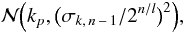 where kp is the parameter value of the parent p, σk,n − 1 the standard deviation of values of the parameter k in the previous generation (n − 1) and l a fixed (positive) number.
The choice of the above standard deviation ensures that we explore the neighborhood of interesting models in a decent way. Parameters that are easily constrained will naturally evolve quicker to their fittest value, and hence the population standard deviation σk,n of the parameter will rapidly diminish. The factor 2n/l will gradually speed up the confinement of the random-pick process. We fix value l = 10, which we found appropriate for getting a sufficiently fast convergence. The number of models per generation is fixed to 200, of which the best 10% is parent for the next generation. We note that parents are also copied to the next generation, assuring that well-fitting individuals are kept in the model population (elitism).
Appendix B: Error estimation
We start from the reasonable assumption of Gaussian errors on the data points. To each data point (xi,yi), we can associate a Gaussian error distribution 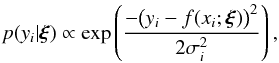 (B.1)where σi is the standard deviation of yi, and f is the model with parameters ξ. The probability associated with the complete data set, i.e., the likelihood function, is then
 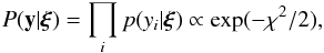 (B.2)i.e., the product of the (independent) probabilities in Eq. (B.1). Here, χ2 follows the classical chi-square definition
  (B.3)In terms of our model fitting, this χ2 corresponds to our χ2 in Eq. (3).
Knowing the likelihood function in Eq. (B.2), we have an estimate on how likely it is to obtain a data set y for a given set of parameters ξ. Bayes’ Theorem allows us then to “flip” this relation, and find the probability distribution of our parameters given our data set, which is what we are actually interested in:  (B.4)Here, P(y) is the probability of the data under all possible model realizations, a factor that can simply be considered as a normalization constant (i.e., independent of ξ). P(ξ), on the other hand, is the prior probability distribution of the parameters. In the absence of any natural preference for the parameters prior to obtaining the data, we can assume flat priors, i.e., uniform probability distributions for each of the parameters. In the range of possible parameter values, Eq. (B.4) thus indicates that P(ξ | y) and P(y | ξ) are identical under our assumptions.
In essence, what we want is to have a sufficient amount of information on our likelihood function, or equivalently on our χ2-function (Eq. (B.2)). Under that condition, we know the behavior of the joint probability distribution P(ξ | y), which implies we can calculate marginal distributions P(ξi | y) for each of the different parameters ξi, and get expectation values and standard deviations. The latter values are then the formal error bars on each of the individual parameters.
Sampling the χ2-function (Eq. (B.2)) can be achieved by calculating models on an extended grid of parameters (e.g., Pinte et al. 2008b; Lebreton et al. 2012). The grid method has the advantage that the parameter space is sampled in a regular way, making it straightforward to calculate the marginal probability distributions of the different parameters. In the case of a genetic fitting algorithm, we indeed also have a sampling of the χ2-function, though very irregular. However, the algorithm will naturally constrain the sampling to the interesting parts of the parameter space, where the sampling is also increased. For a sufficiently converged fitting algorithm, one can therefore imagine the sampling of the algorithm to be good enough for having the necessary information on the χ2-function.
The way we estimate our modeling errors is to make a multi-dimensional interpolation of our exp( − χ2/ 2) values on a parameter grid, normalizing the sum to 1 (in order to get a probability distribution). This is then our estimate of P(ξ | y), which we can marginalize to get the probability distributions for the individual parameters.
Appendix C: Long-wavelength SED
 |
Fig. C.1 Long-wavelength SED of TW Hya, including the new 4.1-cm and 6.3-cm detection. The dashed lines denote the power law fits corresponding to the dust emission (red) and the radio continuum excess (green). The full line is the sum of the two contributions. In gray, a set of 100 models from the Monte Carlo resampling analysis is shown. |
Following the approach of Pascucci et al. (2012), we first fit the (sub-)mm SED with a single power law (Fν ∝ να), corresponding to the optically thin dust emission (Fig. C.1). This gives a spectral index of αmm = 2.47 ± 0.05 (cf. αmm = 2.57 ± 0.06 found by Pascucci et al. 2012). As a second step, we add a second power law to the fit for estimating the excess spectral index αexcess at cm-wavelengths. The resulting spectral slope of the best fit is  . We applied a Monte Carlo resampling technique (see, e.g., Andrae 2010) for inferring the uncertainty on this parameter. The inferred probability distributions for the dust-continuum and radio-excess emission allow us to estimate the contribution of the excess emission to the 9-mm VLA data. The ratio of excess to dust emission at 9.3 mm for the best fit is 3.8%, and it is below 12% at a 95% confidence level.
On the basis of this fit to the radio excess, we thus conclude that dust emission accounts for at least 90% (and likely even more) of the flux observed at 9 mm. In case this emission is free-free thermal emission, the analysis of Pascucci et al. (2012) shows that the expected radio spectral index is αexcess = −0.1. This negative spectral index suggests an even lower contribution of an excess at 9 mm.
In their analysis of the 9-mm VLA data of the T Tauri star AS 209, Pérez et al. (2012) find a point-like contribution to the flux on the level of ~ 10%, which they associate with free-free emission from a compact ionized wind. In our TW Hya data, probing significantly longer baselines, no point-source emission is detected: the averaged visibility on baselines >1400 kλ is effectively zero (0.022 ± 0.024 mJy). Any point-like free-free emission on the level of a few percent is thus excluded.
In a related note, we want to emphasize the interesting behavior of TW Hya’s SED in the centimeter wavelength range and its implication. It was recognized early on that the dust emission of circumstellar disks might be traceable beyond the classical mm wavelength range (λ ≲ 3.4 mm), well into the centimeter regime (e.g., Mundy et al. 1993). In the more recent past, several multi-object studies detected dusty disks at wavelengths between 7 and 16 mm with VLA and with ATCA (e.g., Rodmann et al. 2006; Lommen et al. 2009; Ubach et al. 2012). The detected signals at longer wavelengths (≳2 cm), however, were usually interpreted as arising from an ionized gas component via free-free emission. This was corroborated by the early T Tauri disk models that predicted very low flux densities from dust at a wavelength of 3.6 cm (cf. Beckwith et al. 1990; Mundy et al. 1993). Consequently, Rodmann et al. (2006), for instance, assumed that their 2.0 and 3.6 cm VLA detections arise from free-free emission, and used the resulting spectral index to correct their 7 mm signal for a non-dust contribution. At ATCA, often only upper limits could be established for the flux at 3 and/or 6 cm, preventing a robust derivation of the corresponding spectral index (Lommen et al. 2009; Ubach et al. 2012).
The C-band VLA data we have used for TW Hya consist, as mentioned above, of two sub-bands at 4.8 and 7.3 GHz (6.3 and 4.1 cm). Not only can these two data points be used in the global analysis of the long-wavelength SED as shown above, each of the two sub-bands also covers a 1 GHz-wide bandpass in frequency. The multifrequency synthesis algorithm implemented in CASA allows us to derive a spectral index along such a 1-GHz range. Hence, we can report two additional spectral indices, 1.2 ± 0.6 at 4.8 GHz, and 3.6 ± 0.4 at 7.3 GHz, measured around the intensity peak. The error bars are relatively large, since the total intensity signal of TW Hya at these frequencies is very low. One should therefore not over-interpret the actual values. Still, a qualitatively different behavior is evident. The two spectral indices are different with high confidence, much steeper at 7.3 GHz than at 4.8 GHz. We interpret this finding as an indication that for TW Hya, even at wavelengths as long as 4 cm, the dust emission is detected and has a considerable influence on the spectral index at this frequency. At 6 cm, the relative contribution from the dust might level out with other emission mechanisms and will eventually fade for longer wavelengths.
All Tables
Parameters taken for model reimplementation. Essentially all parameter values are exact copies of the original papers.
Parameter values and estimated uncertainties for the best fit of the different models.
All Figures
|
Fig. 1 Uv-plot of all MIDI observations of TW Hya, distinguishing between the successful (green) and unsuccessful (red) fringe tracks. The curved tracks correspond to the different baselines, with the different names indicated. Clearly, the yellow area with a 50-m radius indicates the domain accessible with MIDI. |
| In the text | |
|
Fig. 2 Comparison of the new VLA data with the previous 7-mm VLA data set of Hughes et al. (2007). The flux for the latter was rescaled applying the spectral index of α = 2.47 to allow the comparison with our 9.315-mm data. Note that the bins for the previous data set are overlapping: only non-adjacent points are effectively independent (see Hughes et al. 2007). |
| In the text | |
|
Fig. 3 Correlated flux at 10 μm for each of the successful MIDI observations, color-coded following the baseline angle at which the observations were done. The baseline-0 observation (black point) corresponds to the average photometric flux of the observations. The full line shows a fit with the correlated-flux profile of an infinitesimally thin ring of angular diameter θ = 26.3 mas (reduced χ2 = 1.54). |
| In the text | |
|
Fig. 4 Comparison of the mass absorption coefficients of the dust mixtures in the different reimplemented models, distinguishing between the inner (dashed) and outer (full) disks. In gray, we show the dust mixture of the final best model (Sect. 6). |
| In the text | |
|
Fig. 5 Comparison of the SED data, the MIDI 50-m visibility profile, the deprojected SMA visibilities, and the deprojected VLA visibilities with the reimplemented model data. Along with the fully reimplemented Calvet et al. (2002) model SED, we show the SED consisting of the sum of the contributions of the inner-disk and the outer-disk SED, for which the radiative transfer is done separately. |
| In the text | |
|
Fig. 6 Model refinement strategy: we start with a simple disk with a vertical inner rim (left), we then introduce a rounded inner rim (middle), and finally also concentrate the largest grains towards the inner disk regions (right). |
| In the text | |
|
Fig. 7 Plots of the best models corresponding to a simple disk (red, dotted), a simple disk with a rounded rim (blue, dashed), and a simple disk with a rounded rim and a centrally-concentrated large grain population (green, full). |
| In the text | |
|
Fig. 8 Convergence plots for Rin (top) and the surface density power p (bottom), for the simple-disk model. The titles of the individual plots indicate to which data set the shown χ2 values correspond (e.g., for MIDI: |
| In the text | |
|
Fig. 9 Mass absorption coefficients per order of magnitude in grain size, for an n(a) ∝ a-3.5 size distribution (within each bin). The vertical lines indicate the wavelengths of the SMA and VLA observations, allowing the comparison of the relative opacity contribution for each of the grain size bins. |
| In the text | |
|
Fig. 10 Current image of the TW Hya transition disk. In black, we represent the centrally concentrated large-grain population, which is also strongly vertically settled. The light-gray outer-disk region between 60 AU and >200 AU is not constrained by our radiative transfer model, but is discussed in Sect. 8.2. We also indicate the regions constrained by the different data sets. The near-infrared data provide only weak constraints (see Sect. 8). |
| In the text | |
|
Fig. 11 PIONIER and NaCo/SAM (squared) visibilities with the predicted visibilities for the final best model (full line), under the approximation of isotropic scattering (red) and full scattering (green; i.e., also including non-isotropic scattering). The dotted green line shows the predictions for the same model, but this time with large grains in the disk atmosphere (simulated by increasing the turbulence strength α from 10-5 to 10-3). Finally, the dashed line again shows the predicted model visibilities of the best model, but now with an outer radius of 200 AU for the < 10-μm sized grains. |
| In the text | |
|
Fig. C.1 Long-wavelength SED of TW Hya, including the new 4.1-cm and 6.3-cm detection. The dashed lines denote the power law fits corresponding to the dust emission (red) and the radio continuum excess (green). The full line is the sum of the two contributions. In gray, a set of 100 models from the Monte Carlo resampling analysis is shown. |
| In the text | |
Current usage metrics show cumulative count of Article Views (full-text article views including HTML views, PDF and ePub downloads, according to the available data) and Abstracts Views on Vision4Press platform.
Data correspond to usage on the plateform after 2015. The current usage metrics is available 48-96 hours after online publication and is updated daily on week days.
Initial download of the metrics may take a while.