| Issue |
A&A
Volume 564, April 2014
|
|
|---|---|---|
| Article Number | A46 | |
| Number of page(s) | 12 | |
| Section | Numerical methods and codes | |
| DOI | https://doi.org/10.1051/0004-6361/201322383 | |
| Published online | 04 April 2014 | |
TAPAS, a web-based service of atmospheric transmission computation for astronomy⋆
1
LATMOS, University of Versailles Saint-Quentin,
11 boulevard d’Alembert,
78280
Guyancourt,
France
e-mail:
This email address is being protected from spambots. You need JavaScript enabled to view it.
2
GEPI, Observatoire de Paris, 5 place Jules Janssen, 92195
Meudon,
France
e-mail:
This email address is being protected from spambots. You need JavaScript enabled to view it.
3
ACRI-ST, BP234, 260 route du Pin Montard,
06904
Sophia-Antipolis,
France
4
IPSL, Institut Pierre-Simon Laplace, Place Jussieu, 75252
Paris,
France
Received: 28 July 2013
Accepted: 3 February 2014
Abstract
Context. Spectra of astronomical targets acquired from ground-based instruments are affected by the atmospheric transmission.
Aims. The authors and their institutes are developing a web-based service, TAPAS (Transmissions Atmosphériques Personnalisées pour l’AStronomie, or Transmissions of the AtmosPhere for AStromomical data). This service, freely available, is developed and maintained within the atmospheric ETHER data center.
Methods. TAPAS computes the atmospheric transmission in the line-of-sight (LOS) to the target indicated by the user. The user files a request indicating the time, ground location, and either the equatorial coordinates of the target or the zenith angle of the LOS. The actual atmospheric profile (temperature, pressure, humidity, ozone content) at that time and place is retrieved from the ETHER atmospheric database (from a combination of ECMWF meteorological field and other information), and the atmospheric transmission is computed from LBLRTM software and HITRAN database for a number of gases: O2, H2O, O3, CO2, CH4, N2O, and Rayleigh extinction. The first purpose of TAPAS output is to allow identifying observed spectral features having an atmospheric or astrophysical origin. The returned transmission may also serve for characterizing the spectrometer on the wavelength scale and instrument line spectral function (ILSF) by comparing one observed spectrum of an atmospheric feature to the transmission. Finally, the top of atmosphere (TOA) spectrum may be obtained either by division of the observed spectrum by the computed transmission or other techniques developed on purpose. The obtention of transmissions for individual species allows more potentialities and better adjustments to the data.
Results. In this paper, we briefly describe the mechanism of computation of the atmospheric transmissions, and we show some results for O2 and H2O atmospheric absorption. The wavelength range is presently 500–2500 nm, but may be extended in the future.
Conclusions. It is hoped that this service will help many astronomers in their research. The user may also contribute to the general knowledge of the atmospheric transmission, if he/she finds systematic discrepancies between synthetic transmissions and the observed spectra. This has already happened in the recent past.
Key words: atmospheric effects / techniques: spectroscopic
© ESO, 2014
1. Introduction
All astronomical targets (stars, galaxies, planets, exoplanets, etc.) are seen from ground-based observatories through the Earth’s atmosphere, which is polluting their spectra. In the field of stellar high-resolution spectroscopy, there is a growing need for an accurate correction of atmospheric transmission, to reach interesting but contaminated spectral regions, to extract the best information from contaminated spectral regions, or simply to make use of them instead of excluding them from analyses.
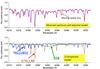 |
Fig. 1 Illustration of data-model adjustment using TAPAS spectra: a high-resolution (R = 65 000) stellar spectrum is shown in the region of the 628.4 nm DIB (top). Data (in red) have been recorded from the Paranal Observatory with the FLAMES-UVES spectrograph at the VLT and adjusted to the convolved product (blue line) of three models shown at bottom: a stellar model computed for the appropriate stellar parameters (brown line), a telluric transmission (blue) and a DIB empirical model (green). The use of the TAPAS transmission allows an optimal adjustment and estimate of the DIB equivalent width. It also allows revealing unambiguously missing lines in the stellar model, such as the feature at 628.7 nm (see Chen et al. 2013). |
To remove the atmospheric absorption features from a scientific target spectrum, one usual technique is to observe a star (a “telluric standard”) close in time and airmass to the scientific target, quite often an early type star and preferably a fast rotator to smooth the few remaining intrinsic lines. Whenever possible, this method has some great advantages over the alternate method that consists in computing a synthetic spectrum of the telluric absorption, as described for TAPAS in the present work. With the “telluric standard” method, there is no need for a good knowledge of the actual quantity of absorbing gas (e.g., water vapor), for an excellent wavelength calibration, and no need for precise knowledge of the ILSF, since absorption features will cancel out when dividing the spectrum of the target by that of the “telluric standard”. (One exception is the case of the use of Adaptive Optics, when the star image may be smaller than the entrance slit of the spectrometer, with a resulting variable ILSF depending on atmospheric conditions, e.g., CRIRES at VLT, Bean et al. 2010.)
However, there are also a number of disadvantages to using a “telluric standard”, as discussed, for instance, in 19: loss of precious observing time, the existence of many stellar features remaining in this template, the impossibility of reaching the true continuum of the target because it is mixed with the one of the bright star, and the absence of feasibility in the case of multi-object spectrographs and weak targets. Today, progress in the molecular databases and radiative transfer models allow improved computations of the atmospheric transmission. Such a synthetic transmission has already been used in the past to correct for water vapor absorption (Lallement et al. 1993); however, a unique transmission spectrum computed for a standard atmosphere was used, adapting to the air mass and humidity by simply amplifying the lines of this unique spectrum. The transmission, however, is a function of the altitude and the atmospheric profile at the observatory. What we propose here is an online tool providing a state-of-the-art computation of this transmission, optimized for the location and time of the observation by using the actual meteorological field from European Center for Medium-range Weather Forecast (ECMWF).
The search for exoplanets by the method of star radial velocity monitoring is extremely demanding in terms of accuracy and cleanliness of stellar spectra. One example is the near-infrared CRIRES radial velocity search with an ammonia cell, as described in Bean et al. (2010). Within the frame of this CRIRES program, Seifahrt et al. (2010) have developed a method of producing synthetic spectra of telluric absorption, which is in many ways similar to the TAPAS method.
There are several ways to use such synthetic atmospheric transmissions: 1) by visual comparison with the target spectrum, to identify telluric features; 2) by fitting the data to a model including the atmospheric transmission, with or without final adjustment to the average airmass and (or) water vapor evolution; 3) by dividing the data with such an optimized transmission template. Important is that our advice for optimal use of the TAPAS tool, for the second and third purposes, is to download the H2O and O2 absorptions spectra separately, which allows refined adjustments and taking the differential behavior of the two species into account at the time of the observations.This is also true for CH4, CO2 and N2O in the near-infrared domain.
An example of using the second method is shown in Fig. 1. The goal was to extract a diffuse interstellar band (DIB), a feature that is imprinted by the intervening interstellar medium in astronomical spectra and is still the object of several studies aiming at identifying its carrier. In the case of the 628.4 nm DIB, strong molecular oxygen lines surround its absorption, which renders the measurement of its equivalent width (EW) difficult, especially for nearby objects (weak DIB), low spectral resolution and high air mass. The O2 transmission is computed with TAPAS for the altitude and location of the observatory (here the ESO Paranal and La Silla observatories in Chile). Figure 1 shows a global adjustment to the data of a combination of stellar, telluric (TAPAS) and diffuse band models (Chen et al. 2013). The choice between the different methods depends on the characteristics of the spectrum and the feature to be observed.
In spectral regions that are highly populated with strong but narrow lines, one can also take advantage of the variable Earth’s velocity on its orbit. Looking at a star (not too far from ecliptic) at various periods, the comb of telluric lines is displaced, and most of the star spectrum may be reconstituted. This method, which was suggested and implemented by one of us (J.L. Bertaux) was first tested for the cool star beta Geminorum, allowing the identification of many molecular lines in the spectrum of the star in the range 930–950 nm (Widemann et al. 1994), where the telluric H2O absorption is severe. The use of TAPAS would allow a better estimate of the depth of these star lines.
The interest of O2 atmospheric lines as a wavelength standard for high-precision measurements of star radial velocities (in search of exoplanets) has also been fostered and tested recently (Figueira et al. 2010). They found that the stability of this atmospheric lines system as measured by HARPS spectrometer at La Silla was better than 10 m/s over six years (10 m/s is 3.3 × 10⁻⁷ c, and corresponds to 1/100 of a pixel in HARPS), which is not surprising, because the wavelengths of the O2 system are dictated by physical laws.
In the next section, we describe the principles of atmospheric transmission calculation used by TAPAS. Then a few examples are shown of correction with TAPAS of three stellar spectra of hot stars taken by three different spectrometers in two regions of the world, in Sects. 3 and 4 for O2 and H2O respectively.
2. TAPAS computation: atmospheric profile and atmospheric transmission
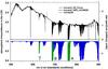 |
Fig. 2 Top panel: spectrum of the star HD 135230 from La Silla, with spectrometer FEROS (ESO) associated to the 2.2 m MPIA telescope. Bottom panel: atmospheric transmittance calculated by TAPAS separately for H2O (blue) and O2 (green) in the range 500–900 nm, at the highest possible resolution with HITRAN. The atmospheric profile was computed for the time of the observation, integrated from the La Silla altitude and with the proper zenith angle. The location of O2 bands are indicated by letters, A, B, γ. The A band is also called the atmospheric band. |
In the visible or near-infrared part of the spectrum, the lines of O2, H2O, and CO2 are the most conspicuous lines affecting the atmospheric transmission (see Fig. 2 for O2 and H2O). Their local absorption depend mainly on the absolute concentration, but also on pressure and temperature. Oxygen is a well-mixed gas and the O2 lines depend on the ground pressure and on the vertical profiles of pressure and temperature. For H2O, the integrated absorption also depends on the vertical distribution of H2O concentration. The TAPAS web service is able to accurately compute the atmospheric transmission from a number of astronomical observatories.
TAPAS is one of the tools developed in the frame of ETHER, a French Atmospheric Chemistry Data Center maintained from CNES and INSU/CNRS funding1. The database includes measurements acquired by satellite, balloons and aircraft, or from other sources, and the aim is to make them available to the entire scientific community for exploitation by modeling or assimilation. ETHER is also a vehicle for discussion and information on related scientific themes that may lead to greater comprehension and better use of existing data. A TAPAS user must be registered once by filling in a form online2.
If the simulated transmission is needed for the future (i.e., for observations planning purposes), TAPAS will use standard atmospheric profiles adequate for the season and latitude of the observatory, stored in the ETHER database. The user may select a standard model in a list of six models, such as “Average latitude summer”. If the simulated transmission is needed to correct a spectrum already acquired in the past, TAPAS will use the most realistic atmospheric profile (temperature T(z) and pressure p(z)) that is available. This atmospheric profile is an ETHER product called Arletty, which is computed by spatial linear interpolation in the grid (1.125° in longitude and latitude) of the ECMWF meteorological field (analysis) for the date and time of the observation. (Actually, there is one field every 6 h, and the one nearest in time to the observation time is selected). For atmospheric levels that are above the highest ECMWF field, Arletty is computing a profile by using the MSISE-90 algorithm (Hedin et al. 1991). Arletty was developed for ETHER by ACRI company from the algorithms of Alain Hauchecorne at LATMOS (Hauchecorne 1999) and is used in many atmospheric projects, i.e., the ENVISAT/GOMOS retrieval of atmospheric constituents from star occultation measurements (Bertaux et al. 2010). The ECMWF data contain also the water vapor and ozone profiles. Water vapor is very important, because it contaminates the spectrum in many wavelength domains with a large number of lines (Fig. 2). Therefore, the input geolocation parameters that have to be entered by the TAPAS user are:
-
the UTC time of the observation;
-
the location of the observer in longitude, latitude, and altitude (a list of selected observatories is available in a roll menu);
-
the RA and Dec of the astronomical target (RA, right ascension, Dec, declination, in the J2000 system). From RA and Dec J2000, TAPAS computes the zenith angle, as an input parameter to the atmospheric transmission. Since an observer may wish to keep confidential its target (defined by RA and Dec), another available option is to give simply the zenith angle and the air mass will be computed by TAPAS.
To compute the atmospheric transmission, TAPAS makes use of Line-By-Line Radiative Transfer Model (LBLRTM; Clough & Iacono 1995) code and the 2008 HITRAN spectroscopic database (this is a high-resolution transmission molecular absorption database3, (16 for the HITRAN 2008), with some improvements from HITRAN 2012, 17. This HITRAN database provides six of the key parameters for each line (or transition), namely the line position, the intensity, the air- and self-broadened halfwidths, the temperature dependence of the air-broadened halfwidth, and the pressure shift of the line. LBLRTM makes use of all these parameters. This is very similar to the method of Seifahrt et al. (2010), which uses HITRAN and LBLRTM, and an atmospheric profile from US National Oceanic and Atmospheric Administration (NOAA), archived in the Global Data Assimilation System (GDAS) available since December 2004 (resolution 1° in longitude and latitude and 3 h in time).
From the user-provided informations, TAPAS computes some other input parameters for LBLRTM, which are
-
the zenith angle,
-
the altitude of the observer,
-
the Arletty p-T vertical profile, and
-
the H2O and ozone profiles from ECMWF.
The atmospheric refraction, which bends the light path and slightly increases the atmospheric path, is taken into account.
Output parameters:
-
1.
Selection of wavelength reference system. The user may select various systems:
-
The wave number system (unit cm-1, wave number = 10 000/wavelength(μm)). It has the advantage of being independent of the air index of refraction.
-
The wavelength in vacuum (unit, nm, nanometer). It is also independent of the air index of refraction.
-
The wavelength (in nm) at 15° C and 760 mm Hg pressure. (It is a commonly used laboratory reference wavelength standard; in particular, lines of thorium argon lamps which are frequently used to calibrate the wavelength scale of spectrometers are given in this particular wavelength reference system.)
It should be noted that the comparison of the observed spectrum, showing numerous O2 or H2O narrow lines, to the TAPAS spectrum may be used to give an uttermost wavelength calibration of the observed spectrum. One thing that is not accounted for in the computation is the wavelength shift due to the Doppler effect induced by the atmospheric wind. Actually, the ECMWF data contain this information and could be used in a future version of TAPAS. With a (high) typical velocity of 20 m/s, it would correspond to a displacement of 1/50 of a pixel for some of the highest dispersion spectrometers found on the astronomical market these days, like HARPS.
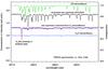
Fig. 3 Green curve: the O2 transmittance computed by TAPAS and convoluted for the appropriate resolution of 44 000, in a narrow spectral interval where O2 lines are present (right scale). Black curve (left scale): the star spectrum showing absorption lines due to telluric O2, shifted from the TAPAS transmission, because the FEROS wavelength calibration put the star spectrum in the barycentric solar system reference. Dark purple curve: star spectrum divided by the convoluted transmittance, after proper wavelength shift (left scale, but vertically displaced for clarity). A conspicuous line remaining corresponds to an O2 line absent from the HITRAN 2008 database. Other small wiggles correspond to weak H2O lines, as indicated by the light blue curve (H2O only TAPAS transmittance, left scale).
-
-
2.
Definition of the spectral interval for the computation. At present, the spectral interval may be selected within the window from 350 to 2500 nm.
-
3.
Selection of atmospheric constituents: the user may select the transmission computation within the following list:
-
Rayleigh extinction, O2, ozone, H2O, CH4, CO2, N2O. In the future, NO2 and NO3 from a climatology established from GOMOS ENVISAT (Bertaux et al. 2010) measurements will also be available. The user may also select the option in which the transmissions are calculated separately for each constituent for a better identification of observed lines. The total transmission is then the multiplication of all individual transmissions. It may also be useful to get the H2O transmission separately, because the quantity of H2O may be adjusted by a power law of the transmission, TX(H2O), where X is the adjusting factor. This may be true for other gases, too.
-
-
4.
The Doppler effect and BERV option.
In the following we examine the spectrum of star HD 135320, which was taken on February 11, 2009, at UTC 09:49:08, with the FEROS high-resolution spectrometer and 2.2 m MPIA telescope at La Silla, an ESO observatory in Chile, and displayed in Fig. 2 (black). This star is a hot star, B9 spectral type, which contains only a limited number of relatively broad stellar spectral lines. The atmospheric transmittance for the relevant atmospheric profile was calculated by TAPAS separately for H2O (blue) and O2 (green) in the range 500–900 nm at the highest possible resolution with HITRAN. The atmospheric absorption lines predicted by the TAPAS model are readily seen on the stellar spectrum.
In Fig. 3 we examine a small 2 nm wavelength interval 627.5–629.6 nm where O2 lines are prominent, by first comparing the star spectrum with the TAPAS O2 only transmittance, convoluted by a Gaussian profile with the FEROS resolution of 44 000. The O2 atmospheric absorption lines are seen in the star’s spectrum, but there is an obvious wavelength shift between the two spectra. This is because the FEROS data reduction pipeline first makes an absolute wavelength calibration (with thorium argon spectral lines delivered by a dedicated lamp). Because of the rotation of the Earth around its spin axis and because of the orbital motion of the Earth around the Sun, there is a Doppler effect along the line-of-sight (LOS) affecting the observed star spectrum. The so-called barycentric earth radial velocity correction (BERV) is applied to the absolute wavelength of the spectrometer, to recover the exact spectrum which would be seen if the observatory were, not on Earth, but rather at the barycenter of the solar system. Since this barycenter has a Galilean motion through the galaxy, all spectra of the same star may be compared to each other even if taken at various times and dates. Small variations in the star’s radial velocities are a major source of exoplanet discoveries, as predicted by 5 and later used with great success (e.g., Mayor & Queloz 1995).
It must be emphasized that the Doppler effect is not a Doppler shift of the wavelength system, but rather a Doppler stretch. The wavelength λ1 after barycentric correction is indeed computed from λ0, absolute calibration of the spectrometer: 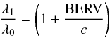 (1)where c is the velocity of light, and BERV = −Vr is the opposite of the radial velocity Vr = dR/dt of the Earth in the direction of the LOS. The convention is that BERV is positive when the Earth is approaching the star (more than the solar system barycenter), while Vr is negative. This change of sign between Vr and BERV is a source of confusion and has unfortunately been the source of many errors in the past. In the case of Fig. 3, BERV was positive (+30.249 km s-1). Therefore, we had to “deberv” the star spectrum by applying an inverse correction (1 – BERV/c) to get it in the observatory/spectrometer system, where the TAPAS transmission is also calculated. Then, the “deberved” star spectrum was divided by the O2-only transmittance spectrum. The result, which in principle represents the star spectrum outside the atmosphere (TOA), is displayed in Fig. 3. There is still a conspicuous line at 627.7 nm. In fact, it is an O2 line which was missing inadvertently in the HITRAN 2008 database, but is present in the 2012 version (Rothman, priv. comm.). Other small wiggles correspond to weak H2O lines, as indicated by the curve of the H2O-only TAPAS transmittance. Instead of changing the star spectrum wavelength scale, one can also stretch the atmospheric transmittances with the same formula (1) that was used (presumably) by the spectrometers data reduction pipeline. TAPAS may do this for the user if desired, provided he/she gives the RA/Dec and time of the observation: the computation of BERV is included in TAPAS. However, this is only an option, because some pipelines do not apply the BERV correction before supplying the reduced spectrum to the observer.
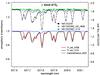 |
Fig. 4 Feros spectrum of star HD 135230, before TAPAS correction (black dots and line, left scale in arbitrary units), and after correction by division of either the HI08 transmittance (red) or the V10 transmittance (black, left scale). There is a clear improvement of the V10 HITRAN O2 database over the earlier HI08 version, as indicated by the flatter green spectrum (corrected with V10) than the blue one (corrected with HI08). The H2O transmittance is indicated by a blue line.The wavelength scale is in nm and in vacuum for this figure and following figures. |
3. Atmospheric transmission of molecular oxygen O2
3.1. General
In the following, we use the TAPAS O2 transmittance to correct a star spectrum by division. In addition to the Feros spectrum of HD 135320, we also used a spectrum of another hot star HD 94756 taken with the NARVAL spectrometer at Pic du Midi (France), with a greater resolution ≃60 000. We examined the three major bands of O2 in the visible in details, namely A (also called “atmospheric band”), B, and γ bands, displayed in Fig. 2. The criterion of goodness is that, after division by the transmittance, the corrected star spectrum should nearly be flat. Of course, when a line is saturated (before instrumental convolution), there is no information on the star spectrum where the transmittance is 0, and there is no hope of retrieving it (except with the technique of several observations throughout the year, see above). However, in many cases, and even on not very saturated lines, we found some remaining spectral features that may be assigned to an improper spectrometer wavelength calibration, an improper line width, or a non-Gaussian ILSF profile. In some other cases, the remaining features do not seem to be connected to instrumental effects.
One caveat is in order here: our method of retrieval of the original spectrum, division by a convoluted transmission, is mathematically incorrect. The mathematically correct method would be to deconvolve the observed spectrum from the ILSF with a considerable wavelength oversampling, and then divide by the transmittance at the highest possible resolution. In practice, however, even with high signal-to-noise-ratio spectra, the data noise would not allow this mathematically correct method. This shortcoming of the division method is obviously more important with strong absorption features than with small ones.
We used three versions of the HITRAN database, hoping that the observations would show improvement with the latest versions. In some cases, later versions are obviously better. In many other cases, we found that the remaining spectral features were much larger than the differences between the various O2 HITRAN databases. The present version of TAPAS is therefore based, for O2, on the latest version contained in the HITRAN web site (December 2012) (except for the continuous absorption, as explained later).
The three versions are:
-
short name HI08: this is the original HITRAN 2008 database;
-
short name V10: HITRAN 2008 plus an update for H2O, O3, and for O2 as discussed in Gordon et al. (2011);
-
short name V11: same as V10 plus a correction for the O2A band of isotopologue 16O16O.
We found that the difference of TAPAS transmittance between V11 and V10 in the A band, after instrumental convolution, was 1.4 × 10⁻³ at most along the A band. In contrast, we found differences in the gamma band of up to 0.02 between V10 and HI08. It may be noted that Gordon et al. (2009) used high-resolution spectra of the Sun, obtained with a Fourier transform spectrometer from TTCON network, at a very high air mass (zenith angle 82.45°) and cold temperature (–23 °C) to minimize water vapor. They were able to adjust some parameters of the B band, in order to reproduce the observation. Their spectral resolution is 0.02 cm-1, or ≃ 700 000 for B band, so much greater than ours. The NARVAL actual spectral resolution was estimated to be ≃60 000 by comparing the observed star spectrum around a strong and isolated O2 line at 769.687 nm to the TAPAS transmittance computed for various resolutions.
3.2. Examination of star spectra divided by the theoretical transmission: the O2 gamma band
The gamma band extends from 627.65 to ≃633 nm and is constituted of a series of relatively weak lines with a maximum depth of 23% at the Feros resolution of 44 000. Figure 4 examines the short wavelength part of the O2 gamma band as seen by the Feros spectrometer. The two versions of the transmittance, HI08 and V10, are indicated, and the two corrected spectra with the two versions.
The corrected spectrum is much flatter for the V10 version, indicating a definite improvement in the line intensity database from HI08 to V10. The remaining spectral feature in the V10-corrected spectrum at 627.8 nm is due to an H2O line. There might still be some undercorrection with the V10 model. We can see that there are still some depressions at the places of some absorption features, which may be used to quantify the deficit of computed absorption. It is well known that the operation of convolution conserves the equivalent width (EW) of an absorption feature. In the regime of weak lines, it can be shown that the EWc of a line in the corrected spectrum is the difference EWm − EWs, where EWm and EWs are the equivalent widths of the weak line, respectively in the measured and the calculated spectrum. Therefore, the EW of the corrected spectrum should be zero if the absorption has been modeled correctly. A deviation from 0 suggests an improper line strength. The correct line strength is the one that would give EWs = EWm.
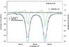 |
Fig. 5 Piece of Narval spectrum of HD 94766 in the B band where two lines of O2 showing shoulders and a self-reversal. The black line with dots is the original spectrum (right scale), the green line with dots is the corrected spectrum after division by the convoluted transmittance. The red line is the TAPAS transmittance convoluted to a resolution of 66 000. The transmittance at high resolution is also plotted (blue), showing that both lines are saturated at the center, and the exact value of the 4 central spectels of the corrected spectrum is somewhat meaningless. There are no H2O absorption features in this range. |
3.3. The O2B band
In Fig. 5 is shown a NARVAL spectrum of two lines of the O2B band, before and after correction by division of the transmittance. Both lines are saturated at center, as indicated by the high-resolution transmittance. For both lines, the corrected spectrum has two shoulders and a strong self-reversal over four points. That the short-wavelength shoulder is higher than the long-wavelength shoulder indicates a small mismatch between the wavelength scales of the transmittance from TAPAS/HITRAN and the observed spectrum. At present we put more confidence in the HITRAN scale than in the spectrometer scale. In order to revise the HITRAN scale, one would have to examine many spectra taken with various spectrometers, and only if a systematic shift was found could one begin to question HITRAN.
At the center of both lines, the self reversal over four “spectels” certainly does not reflect the TOA star spectrum, but is the result of the saturated lines, where the TOA spectrum cannot be retrieved by definition. The self-reversal does not compensate for the shoulders to make EW = 0, but the relationship of EW holding for weak lines does not apply to strong lines, and nothing can be concluded for the true line strength from this non-0 EW. The correct way to check the line strength for strong lines would be to compare directly EWm and EWs (computed with the instrument ILSF and with the same wavelength limits on the EW integral).
While the shoulders (Fig. 5) might be interpreted as an overestimate of this particular line strength in HITRAN, producing an overcorrection, we believe that they are instead a sign that the actual ILSF is slightly narrower in the wings than a Gaussian shape with resolution 60 000, as was taken to compute the TAPAS spectrum. In any case, the corrected spectrum would reveal any stellar feature masked by O2 absorption, except for the four central spectels.
We have also noted that a Feros spectrum in the same region as Fig. 5 shows rather an overcorrection of lines (not shown here), except in a narrow interval, which coincides with a region where the star continuum is higher by 2 to 3%. Indeed, the original spectrum shows a small, but sharp increase at 687.41 nm that cannot be of stellar origin, and is instrumental: possibly an abrupt change in flat field correction, dark charge correction, Stray light removal, or change of grating order. This study case illustrates the potential use of TAPAS to characterize a spectrometer and its pipeline in great detail, not only with the wavelength scale and the ILFS line shape, but also on small photometric features at the 2% level or better.
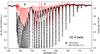 |
Fig. 6 Feros spectrum of star HD 135230 is displayed in the region of O2A band (black dots and line, au), while the TAPAS-corrected spectrum is in red. The two branches P and R of the electronic transition are indicated. See text for discussion. |
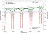 |
Fig. 7 Detail of the P branch in the Feros spectrum of HD 135230: observed (black dots and points), and after correction with TAPAS (green points and line, right scale au). There is a P Cygni pattern in all absorption features. The sign of the P Cygni changes along the spectrum. It goes to zero at 766.5 nm, then reverses its sign, when going from one doublet to the next. There is a line at 766.39 nm in the star spectrum (question mark), not corrected by the atmospheric correction, identified as an interstellar line of potassium at 766.4911nm. |
3.4. The O2 A band
Extending from 759 to 772 nm, this electronic transition of the homopolar O2 molecule is the most conspicuous absorption band in the atmosphere of the Earth in the visible range. Named A band by Fraunhofer, it is also known as “the O2 atmospheric band”. Since O2 is produced by photosynthesis, it should be a prime target for characterizing exoplanets. Though this band is a nuisance for astronomers, it is heavily used in the frame of space-borne Earth observations, either to determine the cloud top altitude, or to determine the effective atmospheric path-length of solar photons scattered by the ground and sent back to space, sometimes after a few scatterings (Rayleigh and aerosols). This allows us to “calibrate” the path-length, and to determine the vertical column density of other molecules, such as CO2, as illustrated by the now flying TANSO/GOSAT experiment or the future OCO-2 satellite. There are no H2O lines in the spectral interval of the O2A band. Provided that the spectral resolution is good enough, the individual lines are separated except at some places in the R branch. Therefore, the use of TAPAS transmission spectra allows the O2 lines to be identified: all other features are genuine. When used in combination with the method of Bertaux (six-months interval star observations), most of the target spectrum may be retrieved, except for stars at high ecliptic latitude where the Doppler effect of the Earth’s orbital velocity becomes negligible.
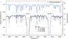 |
Fig. 8 Water vapor lines in the region of D1 and D2 sodium lines. The TAPAS transmission spectrum is in blue, at the top. All lines of the model are seen in the star spectrum. The corrected spectrum has three versions with 3 different resolutions. Regardless of the spectral resolution chosen to compute the TAPAS spectrum, there are residual absorption features that indicate that the quantity of H2O in the model is less than in reality. |
We have tried the three versions of the database, but the model differences are much smaller than some discrepancies between data and model. Therefore, we show only the latest HITRAN version here, V-11, which contained some corrections to the A band (Gordon et al. 2011).
The Feros star spectrum is displayed in Fig. 6 in the domain of the O2A band (Feros data). The overall shape and structure with the two separated branches P and R of the electronic transition is easily captured on the original spectrum. The TAPAS-corrected spectrum is also displayed (with HITRAN version V-11). Many lines are saturated, and the retrieved values at saturated line centers are spurious, and manifested by pseudo-absorption features in the corrected spectrum. Between the lines, the continuum is retrieved well, even in the R branch, where lines are more densely packed.
The upper envelope of the corrected spectrum is slightly depressed with respect to the star continuum outside the band, especially in the R branch. We believe that this is because TAPAS does not yet include an O2 continuous absorption, which was recently added to the HITRAN database (Richard et al. 2012). This is due to collision-induced absorption (CIA), and accounts for O2-O2 as well as O2-N2 and O2-CO2 collisions (Tran et al. 2006).
Figure 7 displays a detail of the P branch with four O2 doublets (Feros spectrum). We note first that all the weak lines other than doublets are corrected well (flat spectrum after correction). The corrected spectrum doublet at 765.5 nm shows a so-called P-Cygni profile (a trough followed by a peak), meaning that there is a slight wavelength shift between data and model. However, there is a progressive change of sign of the P Cygni pattern over a short wavelength interval, from left to right. This is probably the sign of a problem in the wavelength-calibration system of Feros, or its pipeline, rather than a problem in the HITRAN database. It may be due to a CCD engraving problem, which presents some irregularities (called “CCD stitching”, Pasquini 2013, personal communication).
We also note that the positive peak is smaller than the negative peak in the P Cygni profile, indicating that the EW is ≠0. It could mean that these O2 line strengths are actually greater than the HITRAN prediction. However, the absorption lines are strong, and we may be in a situation similar to that of Fig. 5, therefore one would have to consider the EW of data and TAPAS model to check the line strengths.
There is also a line at 766.39 nm in the star spectrum, not corrected by the atmospheric correction. According to one of us (Rosine Lallement), it is an interstellar line of potassium at 766.4911 nm. There is another one at 769.8974 nm that can be seen also in the same Feros spectrum (not shown here). The wavelength shift for the line of Fig. 5 is due to the motion of interstellar material and a Doppler shift of 0.1 nm, corresponding to a heliocentric velocity of 39 km s-1 toward the Sun. It illustrates how the use of TAPAS, by correcting the spectrum and by comparing with the atmospheric transmission alone, may help distinguish between genuine astrophysical absorption features in the observation from atmospheric absorption features. It also illustrates the use of telluric lines for an accurate wavelength calibration, allowing accurate determination of Doppler velocities of interstellar features, well below a small fraction of 1 km s-1. The work of Figueira et al. (2010) is in line with this statement.
4. Water vapor
While O2 is a well mixed gas in the atmosphere, the quantity of water vapor is highly variable in altitude, geography, season, and diurnal cycle. Because it is a tri-atomic molecule, its absorption spectrum is much more complicated than the O2 spectrum (Fig. 2). In the range 0.5–1.0 μm, there are relatively weak lines at many places, and strongly saturated lines at other places. Because of its meteorological interest, weather forecast models and re-analysis include water vapor as a measured, assimilated, and predicted parameter as a function of altitude. Up to now, these models do not include the possibility of a super saturation of water vapor, while tropospheric in-situ measurements sometimes do show such super saturation.
Comparing TAPAS spectra with measured spectra allows determining the quantity of H2O in the atmosphere, and comparing many observations to the ECMWF prediction could perhaps give some clues to super saturation. This is not in the scope of the present paper, where we compare the Feros spectrum to TAPAS output at various places between 500 and 920 nm, stopping short of the strong 936 nm band.
As for O2, the criterium for goodness of fit is that the star spectrum should be as flat as possible after division by the calculated transmission. Figure 8 displays the original star spectrum measured by Feros around the D1 and D2 sodium lines (589 nm), compared to the H2O transmission and divided by the transmission, convoluted with three possible spectral resolutions. It is seen that regardless of the resolution, the corrected spectrum is far from flat, showing a remaining absorption feature at all H2O lines identified in the model. There is an overall deficit with respect to a straight line joining the continua on each side of the group of lines, which suggests that the actual quantity of H2O is more than predicted by TAPAS/ECMWF.
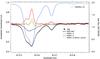 |
Fig. 9 Here, the wavelength shift is very low (no P cygni), therefore the wavelength scale is accurate. The solid black line is the TAPAS corrected with the nominal H2O column. While it is adequate in the H2O line at right, it is not enough for the lines on the left. See text for discussion. The red dotted line is the exact calculation with 1.3 times the nominal H2O column, while the green line is the approximate calculation. There is a significant difference at 915.57 nm where the observed H2O absorption is almost 85%. The TAPAS transmission spectrum is in blue, at the top, left scale, computed for 1.5 the nominal H2O content. |
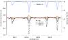 |
Fig. 10 Observed star spectrum (with dots where sampled) corrected from the H2O transmission computed by TAPAS with the nominal value of H2O (black curve), and also with 1.3 (green) and 1.5 the nominal H2O value. The remaining self-reversal is a sign of inadequate resolution/line width. Even over this small spectral interval, it seems that the adequate factor to obtain a featureless spectrum after correction would need a different quantity of H2O: while at 695.36 nm, the factor 1.3 would be approximately correct (green curve), it is too large at 695.64 nm. The TAPAS transmission spectrum is in blue, at the top, left scale, computed for 1.5 the nominal H2O content. |
The presence of weak H2O lines in this range has been a nuisance when differentiating interstellar weak sodium lines from telluric H2O absorptions. However these H2O lines can be used to get an accurate wavelength scale, allowing the Doppler-shift determination (Lallement et al. 1993). To estimate what the transmission should be if the H2O column was changed, we used a method that was used previously by Lallement et al. (1993) to correct even the weak H2O lines. We computed approximate estimates of the transmission by taking the TAPAS nominal transmission (thus, convoluted to the instrument resolution), elevated to the powers 1.1, 1.3 or 1.5. This simulates the case where the distribution of H2O in the atmosphere would be the same as the one selected by TAPAS from ECMWF, multiplied by a factor 1.1, 1.3, or 1.5, which is constant at all altitudes.
This is only an approximation, because the correct calculation would be to use the TAPAS transmission spectrum at the highest resolution, to put it at power X, and then to convolute to the instrument resolution. This correct calculation was done here for the X = 1.3 H2O case, and limited wavelength ranges, in order to check for the difference between exact and approximate calculations (Fig. 9). We have checked that for weak lines, the exact calculation gives similar results to the approximate calculation, which consists of taking the power 1.3 of the convoluted spectrum computed with the nominal resolution. When the H2O absorption is more severe, there is a more noticeable difference between the exact and approximate calculations of the corrected spectrum, as shown in Fig. 9. Therefore, the approximate calculation should be used with caution and only with weak lines (say, giving less than 30% absorption at a resolution of 40 000).
Keeping in mind that the convolution conserves the equivalent width EW, therefore ignoring the self-reversals that are due to an inadequate resolution/ILFS shape, the correct value of X for fitting the corrected star spectrum should display a EW = 0 spectral feature for these relatively weak lines.
Figure 9 is an example where the same quantity of H2O cannot fit two lines that are still very nearby. It is clear that the observed absorption at 915.69 nm is represented fairly well by the nominal H2O value, while this value is too low to represent the absorption observed at 915.55 nm well. Therefore, over very short wavelength intervals, the model absorption requires different amounts of H2O to fit the observed absorptions, which is an unrealistic situation. A similar situation occurs in quite a different wavelength domain, around 695 nm as shown in Fig. 10. The TAPAS-corrected spectra of the same star with Feros are plotted with three values of the multiplying factor X: 1 (nominal case), 1.3 and 1.5. It is clear that that there is not enough water in the nominal case.
A close examination of Fig. 10 indicates that, even over this small spectral interval, the adequate factor X for obtaining a featureless spectrum after correction would need a different quantity of H2O: while at 695.36 nm, the factor 1.3 would be approximately correct, it is too large at 695.64, and perhaps too small for the two other lines at 695.87 and 696.07 nm. This of course does not reflect reality: at a given time and place, there is only one quantity of H2O in the atmosphere.
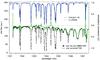 |
Fig. 11 TAPAS comparison to a star spectrum in the near-infrared. The black curve with dots (bottom, left scale) is a spectrum of a B 0.2 V star (tau Sco) acquired by CRIRES at VLT on February 27, 2010, at 09/10/40 UTC (arbitrary unit). Blue curve (top, right scale): TAPAS retrieved atmospheric transmission of H2O with a resolution of 60 000 and a quantity of H2O multiplied by 1.18. Some lines are overcorrected by TAPAS/HITRAN, in particular at 1507.25 nm. Black dashed line: synthetic model from ATRAN web site. One line at 1501.26 nm is absent in ATRAN. The wavelength scale is in nm and in vacuum. |
We have also briefly tested TAPAS in the infrared, with a spectrum of tau Scorpii (HD 149438), a B0.2 V star selected by 11 to produce a library of high-resolution spectra in the near-infrared with the ESO spectrometer CRIRES (VLT), which must be corrected from atmospheric absorption for astrophysical research. A portion (almost one full order) of the spectrum displayed in Fig. 11 (bottom) was retrieved from the CRIRES-POP website4. It is the pipeline-reduced version, and the telluric corrected version is not yet available for this wavelength interval. This spectral region contains moderately strong H2O lines and only tiny CO2 absorption lines, at a level below 0.35%, so are not considered here. Comparing the HITRAN predicted positions of the various H2O lines with observed lines, we had to set up a new wavelength scale with a parabolic fit to HITRAN lines. Then we tested several resolutions and found that 60 000 was giving fair agreement in terms of line profile. Also, the quantity of H2O had to be multiplied by a factor 1.18 to fit most of the observed H2O absorption features. This is in contrast to the finding of Seifahrt et al. (2010), who had to scale down the GDAS predicted amount of H2O by a factor 0.4–0.7 to match the observed H2O lines in the same domain as Fig. 11.
ATRAN is a web-based tool5 for computing the atmospheric transmission online which was developed in the 90s by Steve Lord (1992). It can be therefore considered as an ancestor of TAPAS. ATRAN is limited to the infrared domaine (lambda >0.85 μm). The atmospheric profile is determined from a climatology for five latitudes and no seasonal variation, described by a limited number of atmospheric layers (maximum 5), while TAPAS/LBLRTM considers about 100 layers and a meteorological field. The current spectroscopic database of ATRAN is HITRAN 2000. There is no control on the output resolution for ATRAN. A comparison with TAPAS in the interval 1500–1510 nm indicates similar results (Fig. 11), except that a line at 1501.26 nm, absent in the ATRAN output, is predicted by TAPAS/HITRAN 2012 and indeed observed at the very edge of one CRIRES-POP spectrum at 1501.25 nm (Fig. 11).
A telluric absorption corrected version (Fig. 11, bottom) is obtained by dividing the star spectrum by the transmission (Fig. 11, top). This “true” top of atmosphere (TOA) spectrum contains several pronounced stellar features, in spite of being a hot B0.5 V star, which are sometimes considered as featureless “telluric standard”. This corrected spectrum obviously still contains some artifacts. Some high-frequency wiggles near H2O line centers are probably there because TAPAS only considers Gaussian ILSF, while the actual profile may be more complicated. Three absorption features are overcorrected by TAPAS/HITRAN, at 1502.76 nm, 1504.03 nm, and 1507.25 nm. The ratio of the equivalent widths EWObserved/EWTAPAS are 0.972, 0.906, and 0.21 respectively. The translation of these ratios into line strength would require constructing a curve of growth for each line, well beyond the scope of this paper. Still, it can be stated that the HITRAN strength of the line at 1507.25 nm is greater than it should be by a factor larger than 5.
Besides this exceptional discrepancy, we found two H2O features common to the visible and near-infrared domain. The first feature is that the meteorological prediction of H2O has to be multiplied by a factor that is greater than 1. However, our sample is statistically very limited, and Seifahrt et al. (2010) found factors below 1: 0.4–0.7. Therefore, it cannot be a problem in HITRAN, but is instead a problem in the meteorological model prediction, where the retrieved column of H2O through a fit of spectral telluric absorption is much more accurate than the meteo prediction. The second feature is that over very short wavelength intervals, the HITRAN-based model absorption requires different amounts of H2O to fit the observed absorptions, which is an unrealistic situation. It may be due to shortcomings of the HITRAN database, something that could only be confirmed on the basis of statistical studies with a large number of spectra covering geography, latitude, and time of the year. Another possibility (not exclusive of the first one) is that the actual vertical profile of H2O concentration, temperature, and pressure may be different than a meteorological model (ECMWF, or GADS as discussed in Seifahrt et al. 2010). This may give rise to the observed discrepancies, because the lines parameters depend on these vertical profiles.
Actually, it is conceivable that the series of observed absorptions of O2 and H2O on hot stars over the range 0.5–2.5 μm could be fitted by one single vertical profile of H2O, p and T. This would open the future to a new series of atmospheric parameters that could be assimilated in the weather forecast models, if an adequate real-time pipeline is implemented for this purpose. Additionally, measurements of CH4, CO2, and N2O, which are variable, could be reported to the NDACC system (Network for Detection of Atmospheric Composition Change) for a long term monitoring of these important green house gases. This would require better wavelength calibration and a better knowledge of the instrumental function, most likely variable over the observed wavelength domain. This would be a part of the pipeline and fitting process.
5. Conclusions and perspectives
In this paper we have described the mechanism by which the TAPAS system provides a model of the atmospheric transmission to the user through a simple web interface. This was the main objective of the paper, and we hope that the users will find this new service useful for their astronomical research. Their comments and suggestions will be greatly appreciated, and it is foreseen that TAPAS will evolve in response to the suggestions. As a validation exercise of TAPAS, we used three stellar spectra of hot stars taken by three different spectrometers in two regions of the world, focusing on the absorption of O2 and H2O, and we corrected them with TAPAS transmission spectra. Our findings are as follows:
-
All the lines predicted by TAPAS/HITRAN are indeed present inthe observed spectra. (We have visually scanned the wholespectra up to 900 nm with IGOR software.)
-
The lines observed in the star spectra all come from telluric absorption, except for some well known stellar lines and some interstellar absorption lines.
-
There are some discrepancies in the wavelength scale of the lines (not described by a single shift) that we assign to the spectrometer pipelines.
-
There are some discrepancies in the width and shape of individual lines, because the actual ILSF is different from the assumed Gaussian shape in TAPAS.
-
For H2O, the TAPAS/ECMWF predicted column may be different: 30% ± 10% in our study’s case.
Therefore, TAPAS may be used for the following purposes by the general astronomer user working on a spectrum:
-
1.
identify the telluric origin (atmospheric) of one observedabsorption feature, and assign an astrophysical origin moresafely to the other lines not predicted in TAPAS/HITRAN;
-
2.
identify the atmospheric absorbing gas molecule;
-
3.
establish an accurate wavelength calibration scale of the observed spectrum in the reference system of the spectrometer;
-
4.
determine the spectral resolution of the spectrometer (width of the ILSF);
-
5.
determine the actual ILSF of the spectrometer. The actual ILFS of a spectrometer may be retrieved from a deconvolution of the observed spectrum in the region of a narrow line, as predicted from TAPAS for instance. A deconvolution may be regarded as the solution of a greatly overdetermined linear system. We have tried both the method of least square fitting of the system, and the method of singular value decomposition (SVD) as exposed and recommended by 18. Both methods are working well;
-
6.
correct the observed spectrum from telluric absorption. For H2O, it may need some manipulation outside of the TAPAS environment or several calls to TAPAS to get a good fit for all the lines;
-
7.
use the proposed method (power law) for adjusting the H2O (or other gases) column.
TAPAS should be the most useful on cool stars, where stellar lines are narrow, as for O2 and H2O lines. Since these stars are heavily used in the search for exoplanets, it is particularly interesting to use the atmospheric lines for a wavelength standard (Figueira et al. 2010). Also, if corrected well with TAPAS, some telluric contaminated regions that are presently discarded from the exoplanet search through radial velocity variations could be added to the analysis for a better retrieval of Vr changes.
In the future, TAPAS could be used for characterizing each astronomical hi res spectrometer better, and an improvement of the associated pipelines (wavelength scale, dark charge, sky light and stray light subtraction, spectrum extraction from a 2D image of a cross-dispersed spectrum). The actual ILFS could be determined in a number of spectral intervals and provided with the spectrum as a separated file or in a multifile FITS format. In fact, several of these operations could be included in the reduction pipelines, with an automatic request to TAPAS.
In our test use of TAPAS, we assigned most of the discrepancies to shortcomings of the spectrometers, and not to inaccuracies of HITRAN (wavelength position and strength of lines, and sensitivity to temperature and pressure, excepted for a line at 1507.25 nm). It does not mean there are none, but in order to find them, the discrepancies should be found systematically for various spectrometers at various places and times, taking advantage of the constancy of line spectroscopy, universal and stable. We believe that the HARPS spectrometer at La Silla would be a good additional candidate for such an exercise, given some of the instrumental features: spectrometer under vacuum, fiber-fed with scrambler (stability of ILSF), high spectral resolution, and excellent mechanical stability through accurate temperature control. However, the wavelength domain is limited to 383 to 693 nm.
TAPAS will be improved and maintained by our team. Improvements will occur through corrections of mistakes, as signaled by the users. It is recommended that all users report major mismatches of observed atmospheric lines with the TAPAS calculations, which may result in an improvement of the molecular spectra databases. Also, we will add the O2 continuum absorption following the line described in 15. Then absorption by NO2 and NO3 from a climatology established from GOMOS onboard the ESA ENVISAT spacecraft (Bertaux et al. 2010) measurements may also be available.
As it has been signaled already, line parameters are influenced by temperature and pressure. Therefore, it is possible in theory to determine the vertical profile of H2O, pressure and temperature, by inversing an observation (preferably a spectrum of a hot star). This has already been done with success in the near-infrared (Mumma et al. 2009), in their search for methane
on Mars. The method remains to be demonstrated for the 0.5–1 μm range, where a huge number of spectra are collected, but it could be easier in the range 1.0–2.5 μm. If the inversion is done in near real time, all these vertical profiles could be sent to weather forecast operational centers for assimilation in their models. Satellite borne instruments are doing this from space, but because they look in the nadir direction to the ground, they suffer from the contribution from the Earth’s surface, which is absent in the telescope geometry, looking up. One thing that should be fairly easy to retrieve would be the H2O column, as we have shown in this paper. We suggest that this parameter is an extremely sensitive indicator of surface temperature, because of the Clausius-Clapeyron form of the law of water-vapor saturation versus temperature. Therefore, monitoring the column of water vapor from various observatories could help determine what is the real change in global surface temperature. Combined with the positive feed-back mechanism of water vapor (a temperature increase triggers an increase of H2O, which in turns increases the greenhouse effect and the temperature), it would address one major issue that the world has to face today.
This is done by logging on to ether.ipsl.jussieu.fr/tapas/, then clicking on “connection”. Once registered and getting a password, clicking on “request form” will make the users’ interface window appear.
Acknowledgments
This work is being supported by CNES (Centre National des Études Spatiales) and CNRS (Centre National de la Recherche Scientifique) and its Institut National des Sciences de l’Univers (INSU). It is a collaborative endeavor of LATMOS, GEPI, ACRI and ETHER/IPSL. We acknowledge the use of the HITRAN database and the LBLRTM radiative transfer code, and the use of ECMWF data and the ETHER data center. We acknowledge useful discussions with Larry Rothman and Iouli Gordon, both in Reims and in Boston. We wish to thank the anonymous referee for very useful suggestions. Problems from TAPAS malfunctions should be addressed to Cathy Boonne (IPSL), This email address is being protected from spambots. You need JavaScript enabled to view it. . Other questions should be addressed to one of following emails: This email address is being protected from spambots. You need JavaScript enabled to view it. , or This email address is being protected from spambots. You need JavaScript enabled to view it. .
References
- Bean, J. L., Seifahrt, A., Hartman, H., et al. 2010, ApJ, 713, 410 [NASA ADS] [CrossRef] [Google Scholar]
- Bertaux, J.-L., Kyrola, E., Fussen, D., Hauchecorne, A., et al. 2010, Atmos. Chem. Phys., 10, 12091 [Google Scholar]
- Chen, H.-C., Lallement, R., Babusiaux, C., et al. 2013, ApJ, 550, A62 [Google Scholar]
- Clough, S. A., & Iacono, M. J. 1995, J. Geophys. Res., 100, D8, 16 519 [Google Scholar]
- Connes, P. 1985, Ap&SS, 110, 211 [NASA ADS] [CrossRef] [Google Scholar]
- Figueira, P., Pepe, F, Lovis, C., & Mayor, M. 2010, A&A, 515, A106 [NASA ADS] [CrossRef] [EDP Sciences] [Google Scholar]
- Gordon, I. E., Rothman, L. S., & Toon, G. C. 2011, J. Quant. Spectrosc. Radiat. Transf., 112, 2310 [NASA ADS] [CrossRef] [Google Scholar]
- Hauchecorne, A. 1999, service ARLETTY, description du modèle d’atmosphère, Document interne, réf: ETH-NT-231-TECH-562-SA [Google Scholar]
- Hedin, A. E. 1991, J. Geophys. Res. 96, 1159 [Google Scholar]
- Lallement, R., Bertin, P., Chassefière, E., & Scott, N. 1993, A&A, 271, 734 [NASA ADS] [Google Scholar]
- Lebzelter, T., Seifahrt, A., Uttenthaler, S., et al. 2012, A&A, 539, A109 [NASA ADS] [CrossRef] [EDP Sciences] [Google Scholar]
- Lord, S. D. 1992, NASA Technical Memorandum 103957 [Google Scholar]
- Mayor, M., & Queloz, D. 1995, Nature, 378, 355 [NASA ADS] [CrossRef] [Google Scholar]
- Mumma, M. J., Villanueva, G. L., Novak, R. E., et al. 2009, Science, 323, 1041 [NASA ADS] [CrossRef] [PubMed] [Google Scholar]
- Richard, C., Gordon, I. E., Rothman, L. S., et al. 2012, J. Quant. Spectr. Radiat. Transf., 113, 1276 [NASA ADS] [CrossRef] [Google Scholar]
- Rothman, L. S., Gordon, I. E., Barbe, A., et al. 2009, J. Quant. Spectrosc. Radiat. Transf., 110, 9 [Google Scholar]
- Rothman, L. S., Gordon, I. E., Babikov, Y., Barbe, A., et al. 2013, J. Quant. Spectrosc. Radiat. Transf., 130, 4 [Google Scholar]
- Rucinski, S. 1999, in Precise Stellar Radial Velocities, eds. J. B. Hearnshaw, & C. D. Scarfe, ASP Conf. Ser., 185 [Google Scholar]
- Seifahrt, A., Kaufl, H. U., Zangl, G., Bean, J. L., et al. 2010, A&A, 524, A11 [NASA ADS] [CrossRef] [EDP Sciences] [Google Scholar]
- Tran, H., Boulet, C., & Hartmann, J.-M. 2006, J. Geophys. Res., 111, 15 210 [Google Scholar]
- Widemann, T., Bertaux, J. L., Querci, M., & Querci, F. 1994, A&A, 282, 879 [NASA ADS] [Google Scholar]
All Figures
|
Fig. 1 Illustration of data-model adjustment using TAPAS spectra: a high-resolution (R = 65 000) stellar spectrum is shown in the region of the 628.4 nm DIB (top). Data (in red) have been recorded from the Paranal Observatory with the FLAMES-UVES spectrograph at the VLT and adjusted to the convolved product (blue line) of three models shown at bottom: a stellar model computed for the appropriate stellar parameters (brown line), a telluric transmission (blue) and a DIB empirical model (green). The use of the TAPAS transmission allows an optimal adjustment and estimate of the DIB equivalent width. It also allows revealing unambiguously missing lines in the stellar model, such as the feature at 628.7 nm (see Chen et al. 2013). |
| In the text | |
|
Fig. 2 Top panel: spectrum of the star HD 135230 from La Silla, with spectrometer FEROS (ESO) associated to the 2.2 m MPIA telescope. Bottom panel: atmospheric transmittance calculated by TAPAS separately for H2O (blue) and O2 (green) in the range 500–900 nm, at the highest possible resolution with HITRAN. The atmospheric profile was computed for the time of the observation, integrated from the La Silla altitude and with the proper zenith angle. The location of O2 bands are indicated by letters, A, B, γ. The A band is also called the atmospheric band. |
| In the text | |
|
Fig. 3 Green curve: the O2 transmittance computed by TAPAS and convoluted for the appropriate resolution of 44 000, in a narrow spectral interval where O2 lines are present (right scale). Black curve (left scale): the star spectrum showing absorption lines due to telluric O2, shifted from the TAPAS transmission, because the FEROS wavelength calibration put the star spectrum in the barycentric solar system reference. Dark purple curve: star spectrum divided by the convoluted transmittance, after proper wavelength shift (left scale, but vertically displaced for clarity). A conspicuous line remaining corresponds to an O2 line absent from the HITRAN 2008 database. Other small wiggles correspond to weak H2O lines, as indicated by the light blue curve (H2O only TAPAS transmittance, left scale). |
| In the text | |
|
Fig. 4 Feros spectrum of star HD 135230, before TAPAS correction (black dots and line, left scale in arbitrary units), and after correction by division of either the HI08 transmittance (red) or the V10 transmittance (black, left scale). There is a clear improvement of the V10 HITRAN O2 database over the earlier HI08 version, as indicated by the flatter green spectrum (corrected with V10) than the blue one (corrected with HI08). The H2O transmittance is indicated by a blue line.The wavelength scale is in nm and in vacuum for this figure and following figures. |
| In the text | |
|
Fig. 5 Piece of Narval spectrum of HD 94766 in the B band where two lines of O2 showing shoulders and a self-reversal. The black line with dots is the original spectrum (right scale), the green line with dots is the corrected spectrum after division by the convoluted transmittance. The red line is the TAPAS transmittance convoluted to a resolution of 66 000. The transmittance at high resolution is also plotted (blue), showing that both lines are saturated at the center, and the exact value of the 4 central spectels of the corrected spectrum is somewhat meaningless. There are no H2O absorption features in this range. |
| In the text | |
|
Fig. 6 Feros spectrum of star HD 135230 is displayed in the region of O2A band (black dots and line, au), while the TAPAS-corrected spectrum is in red. The two branches P and R of the electronic transition are indicated. See text for discussion. |
| In the text | |
|
Fig. 7 Detail of the P branch in the Feros spectrum of HD 135230: observed (black dots and points), and after correction with TAPAS (green points and line, right scale au). There is a P Cygni pattern in all absorption features. The sign of the P Cygni changes along the spectrum. It goes to zero at 766.5 nm, then reverses its sign, when going from one doublet to the next. There is a line at 766.39 nm in the star spectrum (question mark), not corrected by the atmospheric correction, identified as an interstellar line of potassium at 766.4911nm. |
| In the text | |
|
Fig. 8 Water vapor lines in the region of D1 and D2 sodium lines. The TAPAS transmission spectrum is in blue, at the top. All lines of the model are seen in the star spectrum. The corrected spectrum has three versions with 3 different resolutions. Regardless of the spectral resolution chosen to compute the TAPAS spectrum, there are residual absorption features that indicate that the quantity of H2O in the model is less than in reality. |
| In the text | |
|
Fig. 9 Here, the wavelength shift is very low (no P cygni), therefore the wavelength scale is accurate. The solid black line is the TAPAS corrected with the nominal H2O column. While it is adequate in the H2O line at right, it is not enough for the lines on the left. See text for discussion. The red dotted line is the exact calculation with 1.3 times the nominal H2O column, while the green line is the approximate calculation. There is a significant difference at 915.57 nm where the observed H2O absorption is almost 85%. The TAPAS transmission spectrum is in blue, at the top, left scale, computed for 1.5 the nominal H2O content. |
| In the text | |
|
Fig. 10 Observed star spectrum (with dots where sampled) corrected from the H2O transmission computed by TAPAS with the nominal value of H2O (black curve), and also with 1.3 (green) and 1.5 the nominal H2O value. The remaining self-reversal is a sign of inadequate resolution/line width. Even over this small spectral interval, it seems that the adequate factor to obtain a featureless spectrum after correction would need a different quantity of H2O: while at 695.36 nm, the factor 1.3 would be approximately correct (green curve), it is too large at 695.64 nm. The TAPAS transmission spectrum is in blue, at the top, left scale, computed for 1.5 the nominal H2O content. |
| In the text | |
|
Fig. 11 TAPAS comparison to a star spectrum in the near-infrared. The black curve with dots (bottom, left scale) is a spectrum of a B 0.2 V star (tau Sco) acquired by CRIRES at VLT on February 27, 2010, at 09/10/40 UTC (arbitrary unit). Blue curve (top, right scale): TAPAS retrieved atmospheric transmission of H2O with a resolution of 60 000 and a quantity of H2O multiplied by 1.18. Some lines are overcorrected by TAPAS/HITRAN, in particular at 1507.25 nm. Black dashed line: synthetic model from ATRAN web site. One line at 1501.26 nm is absent in ATRAN. The wavelength scale is in nm and in vacuum. |
| In the text | |
Current usage metrics show cumulative count of Article Views (full-text article views including HTML views, PDF and ePub downloads, according to the available data) and Abstracts Views on Vision4Press platform.
Data correspond to usage on the plateform after 2015. The current usage metrics is available 48-96 hours after online publication and is updated daily on week days.
Initial download of the metrics may take a while.