| Issue |
A&A
Volume 562, February 2014
|
|
|---|---|---|
| Article Number | A77 | |
| Number of page(s) | 22 | |
| Section | Interstellar and circumstellar matter | |
| DOI | https://doi.org/10.1051/0004-6361/201322646 | |
| Published online | 07 February 2014 | |
Rotationally-supported disks around Class I sources in Taurus: disk formation constraints ⋆,⋆⋆
1
Leiden Observatory, Leiden University, PO Box 9513
2300 RA
Leiden
The Netherlands
e-mail: This email address is being protected from spambots. You need JavaScript enabled to view it.
2
SRON Netherlands Institute for Space Research,
PO Box 800,
9700 AV
Groningen, The
Netherlands
3
Niels Bohr Institute, University of Copenhagen,
Juliane Maries Vej 30,
2100
Copenhagen Ø,
Denmark
4
Centre for Star and Planet Formation, Natural History Museum of
Denmark, University of Copenhagen, Øster Voldgade 5–7, 1350
Copenhagen K,
Denmark
5
Max-Planck-Institut für extraterretrische Physik,
Giessenbachstrasse 1,
85748
Garching,
Germany
Received:
10
September
2013
Accepted:
13
December
2013
Abstract
Context. Disks are observed around pre-main sequence stars, but how and when they form is still heavily debated. While disks around young stellar objects have been identified through thermal dust emission, spatially and spectrally resolved molecular line observations are needed to determine their nature. Only a handful of embedded rotationally supported disks have been identified to date.
Aims. We identify and characterize rotationally supported disks near the end of the main accretion phase of low-mass protostars by comparing their gas and dust structures.
Methods. Subarcsecond observations of dust and gas toward four Class I low-mass young stellar objects in Taurus are presented at significantly higher sensitivity than previous studies. The 13CO and C18O J = 2–1 transitions at 220 GHz were observed with the Plateau de Bure Interferometer at a spatial resolution of ≤0.8″ (56 AU radius at 140 pc) and analyzed using uv-space position velocity diagrams to determine the nature of their observed velocity gradient.
Results. Rotationally supported disks (RSDs) are detected around 3 of the 4 Class I sources studied. The derived masses identify them as Stage I objects; i.e., their stellar mass is higher than their envelope and disk masses. The outer radii of the Keplerian disks toward our sample of Class I sources are ≤100 AU. The lack of on-source C18O emission for TMR1 puts an upper limit of 50 AU on its size. Flattened structures at radii >100 AU around these sources are dominated by infalling motion (υ ∝ r-1). A large-scale envelope model is required to estimate the basic parameters of the flattened structure from spatially resolved continuum data. Similarities and differences between the gas and dust disk are discussed. Combined with literature data, the sizes of the RSDs around Class I objects are best described with evolutionary models with an initial rotation of Ω = 10-14 Hz and slow sound speeds. Based on the comparison of gas and dust disk masses, little CO is frozen out within 100 AU in these disks.
Conclusions. Rotationally supported disks with radii up to 100 AU are present around Class I embedded objects. Larger surveys of both Class 0 and I objects are needed to determine whether most disks form late or early in the embedded phase.
Key words: stars: low-mass / techniques: interferometric / stars: protostars / accretion, accretion disks / ISM: molecules / protoplanetary disks
Based on observations carried out with the IRAM Plateau de Bure Interferometer. IRAM is supported by INSU/CNBRS (France), MPG (Germany) and IGN (Spain).
Appendices are available in electronic form at http://www.aanda.org
© ESO, 2014
Noise levels and beam sizes.
1. Introduction
Rotationally supported accretion disks (RSDs) are thought to form very early during the star formation process (see, e.g., Bodenheimer 1995). The RSD transports a significant fraction of the mass from the envelope onto the young star and eventually evolves into a protoplanetary disk as the envelope dissipates. The presence of an RSD affects not only the physical structure of the system but also the chemical content and evolution as it promotes the production of more complex chemical species by providing a longer lifespan at mildly elevated temperature (Aikawa et al. 2008, 2011; Visser et al. 2011). Although the standard picture of star formation predicts early formation and evolution of RSDs, theoretical studies suggest that the presence of magnetic fields prevents the formation of RSDs in the early stages of star formation (e.g., Galli & Shu 1993; Chiang et al. 2008; Li et al. 2011; Joos et al. 2012). Unstable flattened disk-like structures are formed in such simulations, and indeed, disks in the embedded phase have been inferred through continuum observations (e.g., Looney et al. 2003; Jørgensen et al. 2009; Enoch et al. 2011; Chiang et al. 2012). However, with only continuum data, it is difficult to distinguish between such a feature and an RSD. Thus, spatially and spectrally resolved observations of the gas are needed to unravel the nature of these embedded disks.
Only a handful of studies have explored the change in the velocity profiles from the envelope to the disk with spectrally resolved molecular lines (Lee 2010; Yen et al. 2013; Murillo et al. 2013). It is essential to differentiate between the disk and the infalling envelope through such analysis. This paper presents IRAM Plateau de Bure Interferometer (PdBI) observations of 13CO and C18O J = 2–1 toward four Class I sources in Taurus (d = 140 pc) at higher angular resolution (~0.8″= 112 AU diameter at 140 pc) and higher sensitivity than previously possible. We aim to study the velocity profile as revealed through these molecular lines and constrain the size of embedded RSDs toward these sources.
The embedded phase can be divided into the following stages (Robitaille et al. 2006): Stage 0 (Menv > M⋆), Stage I (Menv < M⋆ but Mdisk < Menv) and Stage II (Menv < Mdisk), where M⋆, Menv and Mdisk are masses of the central protostar, envelop and RSD respectively. This is not to be confused with Classes, which are observationally derived evolutionary indicators (Lada & Wilking 1984; Andre et al. 1993) that do not necessarily trace evolutionary stage due to geometrical effects (Whitney et al. 2003; Crapsi et al. 2008; Dunham et al. 2010). However, since all Class I sources discussed in this paper also turn out to be true Stage I sources, we use the Class notation throughout this paper for convenience.
RSDs are ubiquitous once most of the envelope has been dissipated away (Class II) with outer radius Rout up to approximately 200 AU (Williams & Cieza 2011, and references therein). On the other hand, the general kinematical structure of deeply embedded protostars on small scales is still not well understood. There is growing evidence of rotating flattened structures around Class I sources (Keene & Masson 1990; Hayashi et al. 1993; Ohashi et al. 1997a,b; Brinch et al. 2007; Lommen et al. 2008; Jørgensen et al. 2009; Lee 2010, 2011; Takakuwa et al. 2012; Yen et al. 2013), but the question remains how and when RSDs form in the early stages of star formation and what their sizes are.
Class I young stellar objects (YSOs) are ideal targets to search for embedded RSDs. At this stage, the envelope mass has substantially decreased such that the embedded RSD dominates the spatially resolved CO emission (Harsono et al. 2013). CO is the second most abundant molecule and is chemically stable, thus the disk emission should be readily detected. Furthermore, Harsono et al. (2013) showed that the size of the RSD can be directly measured by analyzing the velocity profile observed through spatially and spectrally resolved CO observations. The sources targeted here are TMC1 (IRAS 04381+2540), TMR1 (IRAS 04361+2547), L1536 (IRAS 04295+2251), and TMC1A (IRAS 04365+2535). These Class I objects have been previously observed by the Submillimeter Array (SMA) and the Combined Array for Research in Millimeter-wave Astronomy (CARMA) at lower sensitivity and/or resolution (e.g., Jørgensen et al. 2009; Eisner 2012; Yen et al. 2013). Embedded rotating flattened structures have been proposed previously around TMC1 and TMC1A (Ohashi et al. 1997a; Hogerheijde et al. 1998; Brown & Chandler 1999; Yen et al. 2013). Thus, we target these sources to determine the presence of Keplerian disks, constrain their sizes near the end of the main accretion phase on scales down to 100 AU and compare this with the dust structure.
1.36 mm continuum properties from elliptical Gaussian fits and derived disk and envelope masses (within 15′′) from fluxes.
This paper is laid out as follows. Section 2 presents the observations and data reduction. The continuum and line maps are presented in Sect. 3. In Sect. 4, disk masses and sizes are obtained through continuum visibility modelling. Position–velocity diagrams are then analyzed to determine the size of rotationally supported disks. Section 5 discusses the implications of the observed rotational supported disks toward Class 0 and I sources. Section 6 summarizes the conclusions of this paper.
2. Observations
2.1. IRAM PdBI observations
The sources were observed with IRAM PdBI in the two different configurations tabulated in Table A.1. Observations with an on-source time of ~3.5 h per source with baselines from 15 to 445 m (11 kλ to 327 kλ) were obtained toward TMC1A and TMR1 in March 2012. Additional track-sharing observations of L1536 and TMC1 were obtained in March-April 2013 with an on-source time of ~3 h per source and baselines between 20 to 450 m (15 kλ to 331 kλ). The receivers were tuned to 219.98 GHz (1.36 mm) in order to simultaneously observe the 13CO (220.3987 GHz) and C18O (219.5603 GHz) J = 2–1 lines. The narrow correlators (bandwidth of 40 MHz ~54 km s-1) were centered on each line with a spectral resolution of 0.078 MHz (0.11 km s-1). In addition, the WideX correlator was used, which covers a 3.6 GHz window at a resolution of 1.95 MHz (2.5−3 km s-1) with 6 mJy beam-1 channel-1 RMS.
The calibration and imaging were performed using the CLIC and MAPPING packages of the IRAM GILDAS software1. The standard calibration was followed using the calibrators tabulated in Table A.1. The data quality assessment tool flagged out any integrations with significantly deviating amplitude and/or phase and the continuum was subtracted from the line data before imaging. The continuum visibilities were constructed using the WideX correlator centered on 219.98 GHz (1.36 mm). The resulting beam sizes and noise levels for natural and uniform weightings can be found in Table 1. The uniform weighted images will be used for the analysis in the image space.
2.2. WideX detections
The WideX correlators cover frequencies between 218.68–222.27 GHz. Strong molecular lines that are detected toward all of the sources within the WideX correlator include C18O 2–1 (219.5603541 GHz), SO 56–45 (219.9488184 GHz), and 13CO 2–1 (220.3986841 GHz). The WideX spectra and integrated flux maps are presented in Appendix C but not analyzed here.
3. Results
3.1. Continuum maps
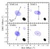 |
Fig. 1 1.36 mm uniform weighted continuum maps toward TMC1A (I4365+2535, top left), TMC1 (I4381+2540, top right), TMR1 (I4361+2547, bottom left), and L1536 (I4295+2251, bottom right). The contours start from 10σ up to 80σ by 10σ. The peak flux densities per beam are 11 mJy, 42 mJy, 23 mJy and 128 mJy for TMC1, TMR1, L1536 and TMC1A, respectively. The red circles indicate the best-fit source-position assuming elliptical Gaussian while the black ellipses show the synthesized beams. The arrows indicate the outflow direction. The RMS is given in Table 1. The dashed blue lines indicate the negative contours starting at 3σ. |
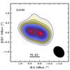 |
Fig. 2 Zoom of the continuum image toward L1536. Both of the line and color contours are drawn at 10% of the peak starting from 4σ up to the peak intensity of 23 mJy beam-1, while the synthesized beam is indicated by the black ellipse in the bottom right corner. |
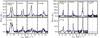 |
Fig. 3 Left: 13CO (top) and C18O 2–1 (bottom) spectra integrated within a 1″ box around the continuum position. Right: single-dish spectra of 13CO 3–2 (except for L1536, which is 13CO 2–1) and C18O 2–1. The vertical red dotted lines indicate the systemic velocities of each source derived from single dish C18O and C17O data (Yıldız et al. 2013). The horizontal blue lines indicate the spectral σrms. |
Strong 1.36 mm continuum emission is detected toward all four sources up to ~450 m baselines (~330 kλ, which corresponds to roughly 80 AU in diameter at the distance of Taurus). To estimate the continuum flux and the size of the emitting region, we performed elliptical Gaussian fits to the visibilities (>25 kλ). The best fit parameters are listed in Table 2. Our derived PdBI 1.36 mm fluxes are <30% lower than the single-dish fluxes tabulated in Motte & André (2001). The only exception is L1536 for which 72% of the singe-dish flux is recovered, which indicates a lack of resolved out large-scale envelope around L1536. The deconvolved sizes indicate a large fraction of the emission is within <100 AU diameter, consistent with compact flattened dust structures.
Figure 1 presents the uniform weighted continuum maps with red circles indicating the continuum positions (Table 2). The total flux of TMC1A is ~30% lower than in Yen et al. (2013) within a 4.0″ × 3.5″ beam, which indicates that some extended structure is resolved-out in our PdBI observations. The peak fluxes of our cleaned maps agree to within 15% with those reported by Eisner (2012) except toward L1536, which is a factor of two lower in our maps. However, our image toward L1536 (Fig. 2) shows that there are two peaks whose sum is within 15% of the peak flux reported in Eisner (2012). The position in Table 2 is centered on the Western peak and the two peaks are separated by ~70 AU. The analysis in the next section (Sect. 4) is with respect to the Western peak. The maps indicate the presence of elongated flattened structure perpendicular to the outflow direction found in the literature (TMC1: 0°; TMR1: 165°; TMC1A: 155°; L1536: None2, Ohashi et al. 1997a; Hogerheijde et al. 1998; Brown & Chandler 1999). Such elongated dust emission is indicative of flattened disk-like structures.
3.2. Molecular lines: maps and morphologies
13CO and C18O 2–1 integrated flux densities [Jy km s-1] within a 5″ box around continuum position.
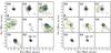 |
Fig. 4 13CO (left) and C18O (right) 2–1 channel maps within the inner 10″ toward TMC1A. The velocities in km s-1 are indicated at the top left in each panel. The contours are drawn at every 3σ starting from 5σ where σ = 12 mJy km s-1 for 13CO and 10 mJy km s-1 for C18O. |
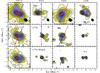 |
Fig. 5 13CO (top) and C18O (bottom) moment zero maps. The contours are drawn at intervals of 10% of the peak starting from 5σ. The continuum position is indicated by the green stars and the arrows show the direction of the red and blue-shifted outflow components taken from the literature (TMC1: 0°; TMR1: 165°; TMC1A: 155°; L1536: None Ohashi et al. 1997a; Hogerheijde et al. 1998; Brown & Chandler 1999). The bottom row show C18O integrated flux maps from the velocity unresolved spectra (typically 1–2 channels) taken within the WideX with contours of 10% of the peak starting from 3σ (~30 mJy beam-1 km s-1). The zero moment maps are obtained by integrating over the velocity ranges [υmin,υmax] = [−3, 11] , [−1, 11] , [−2, 12] , [−2, 12] for TMC1A, TMC1, TMR1, and L1536, respectively. |
 |
Fig. 6 13CO and C18O moment 1 maps within the inner 5″ (700 AU). The solid line indicate the 100 AU scale and the ellipses show the synthesized beams. The gray crosses show the continuum positions. |
The 13CO and C18O 2–1 lines are detected toward all sources. Figure 3 presents the spectra integrated within a 1″ box around the continuum position. The integrated line flux densities within a 5″ box are tabulated in Table 3. The molecular line emission is strongest toward TMC1A and weakest toward L1536, while most of the emission around the systemic velocity is resolved out. This can be seen in the 13CO channel map toward TMC1A (Figs. 3 and 4, see Appendix A for channel maps toward other sources) where most of the emission is absent near υlsr = 6.6 km s-1. In contrast to 13CO, the C18O line is detected around the systemic velocities (±2 km s-1) as shown in Fig. 3 except toward TMC1A, which shows emission within the velocity range comparable to that of 13CO.
Single-dish observations of 13CO J = 3–2 (except for L1536, which is the J = 2–1 transition) and C18O J = 2–1 are also shown in Fig. 3 (right). The comparison indicates that a large part of the emission at the systemic velocity originating from the large-scale envelope is filtered out in our PdBI observations. The PdBI spectra within a 1″ box around each source are also broader than the single-dish spectra. Thus, our PdBI observations are probing the kinematics within the inner few hundreds of AU.
The zeroth moment (i.e., velocity-integrated flux density) maps, are shown in Fig. 5 toward all four sources. The morphologies of the 13CO and C18O maps are different toward 3 out of the 4 sources due to C18O emission being weaker. Only toward TMC1A, which has the strongest C18O emission, do the C18O and 13CO show a similar morphologies. In general, the zeroth moment maps indicate the presence of flattened gas structures that are perpendicular to the outflow direction except for TMR1. In most cases, the C18O emission is weak and compact toward the continuum position as revealed by our higher S/N spectrally unresolved spectra taken with the WideX correlator (bottom panels of Fig. 5).
Moment one (i.e., intensity-weighted average velocity) maps are presented in Fig. 6 and show the presence of velocity gradients in the inner few hundreds of AU. These velocity gradients are perpendicular to the large-scale outflow. Large-scale rotation around TMC1A was reported previously by Ohashi et al. (1997a) extending up to 2000 AU. In addition, Hogerheijde et al. (1998) also detected rotation around TMC1. The high sensitivity and spatial resolution of our observations allow us to map the kinematics on much smaller scales and therefore unravel the nature of these gradients.
4. Analysis
4.1. Continuum: dust disk versus envelope
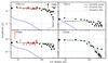 |
Fig. 7 Circularly averaged 1.36 mm visibility amplitudes as function of projected baselines in kλ. The black circles are from this work while the red circles are from previous SMA observations at 1.1 mm (Jørgensen et al. 2009) scaled to 1.36 mm with α = 2.5. The error bars indicate the statistical errors of each bin. The blue line is the simulated continuum emission of the spherical envelope model from Kristensen et al. (2012) sampled using the observed uv points. An arrow in the first panel shows an example of the continuum excess toward TMC1A. Solid squares are the 1.36 mm single-dish flux. The zero-expectation level given in dotted line is the expected amplitude due to noise in the absence of source emission. |
The advantage of an interferometric observation is that one can disentangle the compact disk-like emission from the large-scale envelope. Thus, an estimate of the disk mass can be obtained using both the single-dish and the spatially resolved continuum observations (visibility amplitudes). Figure 7 shows the circularly averaged visibility amplitudes as a function of the projected baselines in kλ (assuming spherically symmetric emission). All sources show strong emission on long baselines that is near constant with increasing baseline. The continuum visibilities of TMR1 and TMC1A are consistent with the scaled (Fν ∝ να) 1.1 mm SMA observations (red circles, Jørgensen et al. 2009) with α = 2.5. An excess of continuum emission at the longest baselines compared with the expected noise is seen toward all sources, which corresponds to unresolved continuum structure at scales smaller than 320 kλ (50 AU radius). Moreover, rapidly increasing amplitudes at short baselines are typically associated with the presence of a large-scale envelope. This combination of features in the visibilities is a typical signature of embedded disks (e.g., Looney et al. 2003; Jørgensen et al. 2005; Enoch et al. 2009).
The first important step is quantifying the large-scale envelope contribution to the uv amplitudes. Using radiative transfer models, Jørgensen et al. (2009) estimated that a spherical envelope contributes at most 4% at 50 kλ at 1.1 mm, which translates to 2% at 1.36 mm. By using the single-dish 850 μm (S15″) and the 50 kλ fluxes (S50kλ), the envelope, Senv, and disk, Sdisk, flux densities can be estimated by solving the following system of equations (Eqs. (2) and (3) in Jørgensen et al. 2009):
We have adopted α ≃ 2.5 to translate the 850 μm disk flux to 1.36 mm (Jørgensen et al. 2007) and c = 0.02 as the fractional envelope contribution. The derived disk masses within 100 AU diameter are tabulated in Table 2 using the OH5 (Ossenkopf & Henning 1994) opacities at 1.36 mm and a dust temperature of 30 K. Our values for TMR1 and TMC1A are consistent with Jørgensen et al. (2009). The envelope masses listed in Table 2 were estimated using Eq. (1) of Jørgensen et al. (2009). Three of the sources (TMC1, TMR1, TMC1A) have similar envelope masses of ~0.1 M⊙, which are higher than the disk masses. In contrast, at most a tenuous envelope seems to be present around L1536. Using the disk to envelope mass ratio as an evolutionary tracer, L1536 is the most evolved source in our sample, which is consistent with its high bolometric temperature. Thus, these sources are indeed near the end of the main accretion phase where a significant compact component is present in comparison to their large-scale envelope.
In interferometric observations toward YSOs, the lack of short baselines coverage may result in underestimation of the large-scale emission and, consequently, overestimating the compact structure. Kristensen et al. (2012) calculated 1D spherically symmetric models derived using the 1D continuum radiative transfer code DUSTY (Ivezic & Elitzur 1997) for a number of sources, including TMC1A, TMR1, and TMC1. The model is described by a power law density structure with an index p (n = n0(r/r0)−p) where n is the number density and with an inner boundary r0 at Tdust = 250 K. The parameters are determined through fitting the observed spectral energy distribution (SED) and the 450 and 850 μm dust emission profiles. These parameters are tabulated in Table B.1. The models in Kristensen et al. (2012) do not take into account the possible contribution by the disk to the submillimeter fluxes and the envelope masses are consequently higher than ours by up to a factor of 2. Using these models, the missing flux can be estimated by modelling the large-scale continuum emission as it would be observed by the interferometer (blue line in Fig. 7). We can therefore place better constraints on the compact flattened structure.
4.2. Constraining the dust disk parameters
The goal of this section is to estimate the size and mass of the compact flattened dust
structure or the disk using a number of more sophisticated methods than Eqs. (1) and (2)
to compare with the estimates from the gas in the next section. We define the disk
component to be any compact flattened structure that deviates from the expected continuum
emission due to the spherical envelope model. In the following sections, the disk sizes
will be estimated by fitting the continuum visibilities with the inclusion of emission
from the large-scale structure described above. As the interferometric observation
recovers a large fraction of the single-dish flux toward L1536, its large-scale envelope
contribution is assumed to be insignificant, and therefore not included. The best-fit
parameters are found through χ2 minimization on the binned
amplitudes. The range of values of Rdisk,
Mdisk, i and PA shown in Table 4 correspond to models with
χ2 between  and
and
 .
.
Disk sizes and masses derived from continuum visibilities modelling using uniform, Gaussian and power-law disk models.
4.2.1. Uniform disk
The first estimate on the disk size and mass is obtained by fitting a uniform disk
model assuming optically thin dust emission (see Fig. 8, Eisner 2012). Uniform disks are
described by a constant intensity I within a diameter
θud whose flux is given by
 . The visibility amplitudes are given by:
 (3)where J1 is the
Bessel function of order 1 and ruv is the projected baseline
in terms of λ. Deprojection of the baselines follow the formula given
in Berger & Segransan (2007):
(3)where J1 is the
Bessel function of order 1 and ruv is the projected baseline
in terms of λ. Deprojection of the baselines follow the formula given
in Berger & Segransan (2007):
 where PA is the position angle (East of
North) and i is the inclination.
where PA is the position angle (East of
North) and i is the inclination.
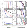 |
Fig. 8 Left: normalized intensity profiles for the three different continuum models: Uniform disk (top), Gaussian Disk (middle), and power-law disk (bottom). Right: normalized visibilities as function of uv radius. For comparison, the L1536 binned data are shown in gray circles. |
The best fit parameters are tabulated in Table 4
with disk masses estimated using a dust temperature of 30 K and OH5 opacities (Table 5
of Ossenkopf & Henning 1994) within
 radius. The disk radii vary between 7 to
171 AU. The smallest disk size is found toward TMR1, which suggests that most of its
continuum emission is due to the large-scale envelope. Moreover, disk sizes around TMR1
and TMC1A are 65%–90% lower than those reported by Eisner (2012, Table 3) since we have included the spherical envelope
contribution. This illustrates the importance of including the large-scale contribution
in analyzing the compact structure.
radius. The disk radii vary between 7 to
171 AU. The smallest disk size is found toward TMR1, which suggests that most of its
continuum emission is due to the large-scale envelope. Moreover, disk sizes around TMR1
and TMC1A are 65%–90% lower than those reported by Eisner (2012, Table 3) since we have included the spherical envelope
contribution. This illustrates the importance of including the large-scale contribution
in analyzing the compact structure.
4.2.2. Gaussian disk
The next step is to use a Gaussian intensity distribution, which is a slightly more
realistic intensity model that represents the mm emission due to an embedded disk. The
visibility amplitudes are described by the following equation:
 (7)where θG is the
FWHM of the Gaussian distribution and F is the total
flux.
(7)where θG is the
FWHM of the Gaussian distribution and F is the total
flux.
The difference between the Gaussian fit presented in Table 2 and this section is the inclusion of the large-scale emission. In Table 2, the Gaussian fit gives an estimate of the size of emission in the observed total image, while this section accounts for the simulated large-scale envelope emission in order to constrain the compact flattened structure. The free-parameters are similar to the uniform disk except that the size of the emitting region is defined by full-width half maximum (FWHM). For a Gaussian distribution, most of the radiation (95%) is emitted from within 2σG ~ 0.85 × FWHM, thus we define the disk radius to be 0.42 × FWHM. The best-fit parameters are tabulated in Table 4 and the corresponding emission is included in Fig. 7. The resulting disk sizes are slightly lower than those derived using a uniform disk.
The visibility amplitudes in Fig. 7 show the presence of an unresolved point source component at long baselines indicated by the arrow in the first panel. Jørgensen et al. (2005) noted that a three components model (large-scale envelope + Gaussian disk + point-source) fits the continuum visibilities. By using such models, the disk sizes generally increase by 20–30 AU with the addition of an unresolved point flux, which is comparable to the uniform disk models. Such models were first introduced by Mundy et al. (1996) since the mm emission seems to be more centrally peaked than a single Gaussian. The unresolved point flux is more likely due to the unresolved disk structure since the free-free emission contribution is expected to be low toward Class I sources (Hogerheijde et al. 1998).
Derived disk sizes and stellar masses from the break radius in the uv-space PV diagrams corrected for inclination.
4.2.3. Power-law disk
The next step in sophistication is to fit the continuum visibilities with a power-law
disk structure. The difference is that the first two disk models are based on the
expected intensity profile of the disk, while the power-law disk models use a more
realistic disk structure. Similar structures were previously used by Lay et al. (1997, see also Lay et al. 1994; Mundy et al.
1996; Dutrey et al. 2007; Malbet et al. 2005. We adopt a disk density structure
described by
Σdisk = Σ50 AU(R/50 AU)−p
where Σ50 AU is the surface density at 50 AU with a temperature structure
given as
Tdisk = 1500(R/0.1 AU)−q.
The inner radius is fixed at 0.1 AU with a dust sublimation temperature of 1500 K, while
the disk outer radius is defined at 15 K. The free parameters are p,
q, Σ50 AU, i and PA where
i is the inclination with respect of the plane of the sky in degrees
(0° is face-on) and PA is the position angle (East of North). The visibilities are
constructed by considering the flux from a thin ring given by:
 (8)where d is the distance,
i is the inclination (0° is face-on),
(8)where d is the distance,
i is the inclination (0° is face-on),
 is the optical depth and
Bν(T) is the Planck
function. For the dust emissivity (κ), we adopt the OH5 values. Since
the model is axisymmetric, the visibilities are given by a one-dimensional Hankel
transform which is given by the analytical expression:
is the optical depth and
Bν(T) is the Planck
function. For the dust emissivity (κ), we adopt the OH5 values. Since
the model is axisymmetric, the visibilities are given by a one-dimensional Hankel
transform which is given by the analytical expression:
 (9)where J0 is the
Bessel function of order 0. The total amplitude at a given
ruv is integrated over the whole disk.
(9)where J0 is the
Bessel function of order 0. The total amplitude at a given
ruv is integrated over the whole disk.
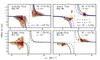 |
Fig. 9 13CO position velocity diagrams along the direction perpendicular to the outflow: TMC1A (top left), TMC1 (top right), TMR1 (bottom left), and L1536 (bottom right). The color contours start from 3σ and increase by 1σ while the black line contours are drawn at 5σ, 8σ, 11σ, and so on up to the peak intensity. The black solid curves show the best-fit Keplerian curves, while the dashed lines indicate the r-1 curves. For TMC1A and TMC1 (top row), the blue solid line presents a 0.4 M⊙ Keplerian curve. |
The first advantage of such modelling is the treatment of the optical depth which gives better mass approximations. Secondly, the unresolved point-flux is already included in the model by simulating the emission from the unresolved disk component. Figure 8 shows the normalized visibilities for a fixed p = 0.9 and a number of Rdisk. The best-fit parameters are tabulated in Table 4.
The derived disk masses obtained by integrating out to ~50 AU radius are similar to those from the 50 kλ point (Table 2). This is expected as the 1.3 mm continuum emission (κOH5 = 0.83 cm2 g-1) is on average nearly optically thin (Jørgensen et al. 2007). The optical depth can be up to 0.4 at radii <10 AU for the best-fit power-law disk models with i > 70°. A wide range of “best-fit” masses is found toward TMR1, which is mainly due to the uncertainties in the inclination.
More recently, Eisner (2012) presented embedded disk models derived from continuum data by fitting the I band image, SED and 1.3 mm visibilities. Our continuum disk radii toward TMC1A and TMR1 are consistent with their results. However, the high quality of our data allow us to rule out disks with Rout > 100 AU toward TMR1. On the other hand, our disk radius toward L1536 is a factor of 3 higher than that reported in Eisner (2012) due to the difference in the treatment of the large-scale envelope.
In summary, different methods have been used to constrain the disk parameters from thermal dust emission. The first two models, Gaussian and uniform disk models, are based on the intensity profile, while the power-law disk models use a simplified disk structure with given density and temperature profiles. The intensity based models find the smallest disk sizes, while the power-law disk models predict up to a factor of two larger disk sizes. On the other hand, the disk masses from these fitting methods are similar. The advantage of the power-law disk modeling is the determination of the density and temperature structures including the unresolved inner part of the disk. The continuum images provide no kinematic information, however, so the important question is whether these flattened structures are rotationally supported disks and if so, whether the continuum sizes agree with those of RSDs.
4.3. Line analysis: Keplerian or not?
The nature of the velocity gradient can already be inferred from the moment maps. First, the 13CO integrated flux maps shown in Fig. 5 indicate the presence of flattened gas structures perpendicular to the outflow direction. Second, the velocity gradient is also oriented perpendicular to the outflow within hundreds of AU, which is a similar size scale to the compact dust structure measured in Sect. 4.2. On the other hand, the velocity gradient does not show a straight transition from the red to the blue shifted component as expected from a Keplerian disk. Taking TMC1A as an example, the blue-shifted emission starts at the North side and skews inward toward the continuum position. Such a skewed moment 1 map is expected for a Keplerian disk embedded in a rotating infalling envelope (Sargent & Beckwith 1987; Brinch et al. 2008). Thus, the moment maps indicate the presence of a rotating infalling envelope leading up to a rotationally dominated structure.
In image space, position velocity (PV) diagrams are generally used to determine the nature of the velocity gradient. Analysis of such diagrams starts by dividing it into four quadrants around the υlsr and source position. A rotating structure occupies two of the four quadrants that are symmetric around the center, while an infalling structure will show emission in all quadrants (e.g., Ohashi et al. 1997a; Brinch et al. 2007). In addition, one can infer the presence of outflow contamination by identifying a velocity gradient in PV space along the outflow direction (e.g., Cabrit et al. 1996).
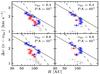 |
Fig. 10 C18O uv-space PV diagrams toward TMC1A with PA = 55°,65° and υlsr = 6.6,6.4 km s-1. The solid lines are the r-0.5 curves and dashed lines are the r-1 curves. The red and blue colors indicate the red- and blue-shifted components, respectively. Gray points show the rest of the peaks that were not included in the fitting. |
Figure 9 presents PV diagrams at a direction perpendicular to the outflow direction; for L1536, the direction of elongation of the continuum was taken. In general, the PV diagrams are consistent with Keplerian profiles, except for TMR1. The PV diagram toward TMR1 seems to indicate that the 13CO line is either dominated by infalling material or the source is oriented toward us, which is difficult to disentangle. However, recent 12CO 3–2 and 6–5 maps presented in Yıldız et al., (in prep.) suggest that the disk is more likely oriented face-on (i < 15°). Furthermore, a velocity gradient is present in the 13CO PV analysis both along and perpendicular to the outflow direction indicating minor outflow contamination for this source.
The focus of this paper is to differentiate between the infalling gas and the rotationally supported disk. Such analysis in image space is not sensitive to the point where the infalling rotating material (υ ∝ r-1) enters the disk and becomes Keplerian (υ ∝ r-0.5). Thus, additional analysis is needed to differentiate between the two cases.
As pointed out by Lin et al. (1994), infalling gas that conserves its angular momentum exhibits a steeper velocity profile (υ ∝ r-1) than free-falling gas (υ ∝ r-0.5). In the case of spectrally resolved optically thin lines, the peak position of the emission corresponds to the maximum possible position of the emitting gas (Sargent & Beckwith 1987; Harsono et al. 2013). On the other hand, molecular emission closer to the systemic velocity is optically thick and, consequently, the inferred positions are only lower limits. Thus, with such a method, one can differentiate between the Keplerian disk and the infalling rotating gas. Moreover, Harsono et al. (2013) suggested that the point where the two velocity profiles meet corresponds to the size of the Keplerian disk, Rk. In the following sections, we will attempt to constrain the size of the Keplerian disk using this method, which we will term the uv-space PV diagram.
The peak positions are determined by fitting the velocity resolved visibilities with Gaussian functions (Lommen et al. 2008; Jørgensen et al. 2009). It can be seen from the channel maps (Fig. 4 and Appendix A) that a Gaussian brightness distribution is a good approximation in determining the peak positions of the high velocity channels.
To characterize the profile of the velocity gradient, the peak positions are projected
along the velocity gradient. This is done by using the following transformation
 where x,y are the peak
positions and
xθ,yθ
are the rotated positions. A velocity profile
(υ ∝ r−η) is then fitted
to a subset of the red- and blue-shifted peaks to determine the best velocity profile.
where x,y are the peak
positions and
xθ,yθ
are the rotated positions. A velocity profile
(υ ∝ r−η) is then fitted
to a subset of the red- and blue-shifted peaks to determine the best velocity profile.
4.3.1. TMC1A
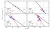 |
Fig. 11 13CO uv-space PV diagrams toward all sources with the best fit profiles superposed in black lines (except for L1536). The red lines indicate a υ ∝ r-1 as comparison. Gray points show the peaks that were not included in the fitting. |
TMC1A shows the greatest promise so far for an embedded Keplerian disk around a Class I protostar . The moment 1 maps (Fig. 6) indicate a gradual change from blue- to red-shifted gas in the inner few hundreds of AU, which is consistent with a Keplerian disk. Figure 10 presents the C18O velocity profiles using the nominal υlsr and PA perpendicular to the outflow direction along with small deviations from those values, which correspond to the uncertainty in outflow direction. In the absence of foreground clouds, one expects that the blue and red-shifted peaks overlap for a rotating system, which is the case if one adopts υlsr = + 6.4 km s-1. The C18O and C17O observations presented in Jørgensen et al. (2002) indicate a υlsr = + 6.6 km s-1, however υlsr = + 6.4 km s-1 is consistent with the N2H+ observations toward the nearby L1534 core (Caselli et al. 2002). For comparison, the 13CO velocity profile with υlsr = + 6.4 km s-1 and PA perpendicular to the outflow direction is shown in Fig 11. Both of the 13CO and C18O lines show a velocity profile close to υ ∝ r-0.5, which indicates that the gas lines trace similar rotationally supported structures. The typical uncertainty in the power-law slope is ± 0.2. In the region where the red- and blue-shifted peaks overlap, a clear break from r~−0.5 to a steeper slope of r-1 can be seen at ~100 AU. This break may shift inward at other PAs and υlsr to 80 AU. However, it is clear that the flattened structure outside of 100 AU flattened structure is dominated by infalling rotating motions. Thus, the embedded RSD toward TMC1A has a radius between 80–100 AU.
To derive the stellar mass associated with the rotationally dominated region,
simultaneous fitting to the PV diagrams in both image and uv space has
been performed. The best-fit stellar mass associated with the observed rotation toward
TMC1A is 0.53 M⊙ at
i = 55° ± 10°.
M⊙ at
i = 55° ± 10°.
Additional analysis is performed for TMC1A with a simple radiative transfer model to
confirm the extent of the Keplerian disk following a method similar to that used by
Murillo et al. (2013) for the VLA 1623 Class 0
source. Such fitting is only performed for this source to investigate whether they give
similar results. A flat disk model given by:  where N is the gas column
density with T0 and N0 as the
reference gas temperature and column densities, respectively, at the reference radius,
r0. Similar to the power-law disk models in Sect. 4.2.3, we have used
T0 = 1500 K at r0 of 0.1 AU. The
images are then convolved with the clean beams in Table 1. We have assumed i = 55° and PA = 65°. For such
orientation, we find that a Keplerian structure within the inner 100 AU is needed,
surrounded by a rotating infalling envelope. The radius of the Keplerian structure is
similar to the radius derived from previous methods (~100 AU), however, a stellar
mass of 0.8 ± 0.3 M⊙ is needed to reproduce the observed
molecular lines. This is consistent with Yen et al.
(2013) calculated at i = 30°, but a factor of 1.5 higher than
the value obtained earlier (although the two values agree within their respective
uncertainties).
where N is the gas column
density with T0 and N0 as the
reference gas temperature and column densities, respectively, at the reference radius,
r0. Similar to the power-law disk models in Sect. 4.2.3, we have used
T0 = 1500 K at r0 of 0.1 AU. The
images are then convolved with the clean beams in Table 1. We have assumed i = 55° and PA = 65°. For such
orientation, we find that a Keplerian structure within the inner 100 AU is needed,
surrounded by a rotating infalling envelope. The radius of the Keplerian structure is
similar to the radius derived from previous methods (~100 AU), however, a stellar
mass of 0.8 ± 0.3 M⊙ is needed to reproduce the observed
molecular lines. This is consistent with Yen et al.
(2013) calculated at i = 30°, but a factor of 1.5 higher than
the value obtained earlier (although the two values agree within their respective
uncertainties).
4.3.2. TMC1
 |
Fig. 12 C18O uv-space PV diagrams toward TMC1 derived from the emission peaks. The solid line indicates the best-fit power-law slope to the peaks between 1.3–1.9 km s-1. The vertical blue dotted lines indicate the 150 AU radius. The red and blue colors indicate the red- and blue-shifted components, respectively. |
The velocity profile for TMC1 projected along PA = 90° is shown in Fig. 11 for 13CO. The moment maps toward this
source indicate the presence of a compact flattened structure around the continuum
position. Similar to TMC1A, the PV diagram also indicates a rotationally dominated
structure. However, in contrast to TMC1A, the 13CO line is best described by
an r-1 profile indicating that it traces infalling rotating
gas, while the C18O line is fitted well with a
r-0.5 slope as shown in Fig. 12 indicative of an RSD. Such discrepancy can occur if the two lines
are tracing different regions. The moment zero maps in Fig. 5 already gave some indication that the 13CO and
C18O emissions do not arise from similar structure. Furthermore, the disk
mass toward TMC1 as inferred through the continuum is the lowest in our sample, hence it
is also possible that the embedded RSD is not massive enough to significantly contribute
to both the 13CO and C18O emission. The relatively more optically
thick 13CO traces the inner envelope and thus is dominated by its kinematics,
while the rotationally supported structure significantly contributes to the
C18O line. A smooth extrapolation of the envelope down to 100–150 AU scales
predicts C18O emission <18% of the observe emission at >1.5
km s-1, suggesting that the majority of the emission at these velocities
originates in a disk (see also models by Harsono et al.
2013, Fig. 8). Hence, using the C18O line, the fit indicates the
presence of an RSD extending between 100−150 AU in radius. The best-fit stellar mass is
0.54M⊙ at
i = 55° with typical error of ±0.2 km s-1 on the
determination of υlsr. The stellar mass is a factor of 1.5
lower than that previously derived by Hogerheijde et al.
(1998) as indicated by the black lines in Fig. 9. However, a stellar mass of 0.4 M⊙ also
reasonably fits the 13CO PV diagram. In addition, the discrepancy between the
13CO and C18O velocity profiles may suggest that the most stable
RSD is less than the C18O break point. Thus, we will use 100 AU as the size
of the RSD toward TMC1.
4.3.3. TMR1
The determination of the velocity profile toward TMR1 is difficult. Adopting υlsr = + 6.3 km s-1 (Kristensen et al. 2012; Yıldız et al. 2013), the red-shifted peaks do not coincide with the blue-shifted peaks as expected from a symmetric rotating infalling structure in the absence of foreground clouds. The 13CO velocity profile is uncertain with a slope between 0.5 to 1 (Fig. 11). However, a velocity gradient is present in the PV analysis along and perpendicular to the outflow direction, which suggest outflow contamination toward TMR1. With the 5σ threshold used for this analysis, only 3 peaks are available in the C18O line, which are located along the blue outflow lobe as inferred from the 12CO J = 3–2 and J = 6–5 maps in Yıldız et al. (in prep.). The on-source C18O line is detected within the WideX correlator, which is double peaked within 100 AU diameter (Fig. 5). Thus, the non-detection of the turn-over from r-1 to r-0.5 indicates that the disk is much smaller than the synthesized beam (<0.7″ = 98 AU diameter). Also, the RSD has to be less massive than TMC1 and TMC1A due to the lack of on-source C18O emission and rotational motion. Thus, the compact flattened dust structure at >50 kλ toward this source cannot be fully associated with an RSD. The molecular emission from TMR1 must be mostly due to the infalling rotating envelope and the entrained outflow gas similar to the conclusion of Jørgensen et al. (2009).
4.3.4. L1536
Figure 11 shows the uv-space PV diagram with systemic velocity of υlsr = +5.3 km s-1. The peak positions were shifted to the center of the two peaks seen in the continuum (Fig. 2) and the C18O integrated map (Fig. 5). The dominant motion at low velocity offsets (Δυ = ±2 km s-1) is infall, while a flatter slope with a power-law close to r-0.5 best describes the high velocity components. If the peak positions were not shifted, only the blue-shifted peaks follow the r-0.5 profile starting from 70–80 AU. The flat velocity profile is based on 4 points and it does not show a very clear Keplerian disk profile such as seen toward TMC1A. From the high velocity peaks, the velocity profile seems to indicate a break at ~80 AU.
4.4. Summary and stellar masses
Three out of the four Class I sources show clear indications of embedded RSDs. From the turn-over radius (from r-1 to r-0.5), the radii of the Keplerian disks must be between 100–150 AU in TMC1, 80 AU toward L1536 and 100 AU toward TMC1A. Considering that the turnover radius is the outer radius of the embedded Keplerian disk, the stellar masses are derived from that radius and tabulated in Table 5. In the case of L1536, we chose the red-shifted peak (~3 km s-1) at 70 AU as the turnover radius to determine the combined stellar masses. Thus, by obtaining the masses of the different components (envelope, disk, and star), it is now possible to place the sources in an evolutionary stage for comparison with theoretical models. The three sources are indeed in Stage I of the embedded phase, where the star has accreted most of its final mass.
The uv-space PV diagram assumes that the disk rotation is perpendicular to the outflow direction as inferred from large 12CO maps, foreground clouds do not contaminate the molecular lines, and the source systemic velocity is well determined. Small systemic velocity shifts can indeed shift both the red-shifted and blue-shifted velocity profiles from r-0.5 to a steeper slope. However, for the firm detection of an embedded RSD toward TMC1A, this does not significantly affect the break radius. Further observations at higher resolution and sensitivity are certainly needed to confirm the extent of the Keplerian disks toward all of these sources. However, we argue that even with the current data it is possible to differentiate the RSD from the infalling rotating envelope with spatially and spectrally resolved molecular line observations.
4.5. Disk gas masses
After determining the extent of the embedded Keplerian disks, their gas masses can be
estimated from the C18O integrated intensities. The J=2–1 line
is expected to be thermalized at the typical densities
(nH2 > 107 cm-3) of
the inner envelope due to the low critical density. The gas mass assuming no significant
freeze-out is then given by the following equation (Scoville et al. 1986; Hogerheijde et al.
1998; Momose et al. 1998):
 (14)where h and
k are natural constants, Tex is the
excitation temperature, τ is the line optical depth,
Eu is the upper energy level in K and
(14)where h and
k are natural constants, Tex is the
excitation temperature, τ is the line optical depth,
Eu is the upper energy level in K and
 is the integrated flux densities in Jy km
s-1 using a distance of 140 pc. The gas mass estimates of the disks inferred
by integrating over a region similar to the extent of RK in
Table 5 are listed in Table 6 with τ = 0.5 and Tex = 40
K. The adopted excitation temperature comes from the expected C18O rotational
temperature within a 1″ beam if a disk dominates such emission (Harsono et al. 2013). From the observed
is the integrated flux densities in Jy km
s-1 using a distance of 140 pc. The gas mass estimates of the disks inferred
by integrating over a region similar to the extent of RK in
Table 5 are listed in Table 6 with τ = 0.5 and Tex = 40
K. The adopted excitation temperature comes from the expected C18O rotational
temperature within a 1″ beam if a disk dominates such emission (Harsono et al. 2013). From the observed
 flux ratios, the
 is estimated to be ≤4.0 with isotopic
ratios of 12C/13C = 70 and 16O/18O = 550
(Wilson & Rood 1994). This implies that the
C18O is almost optically thin
(τC18O ≤ 0.5) and only a small correction is needed
under the assumption that 13CO and C18O trace the same structure.
Uncertainties due to the combined Tex and τ
result in a factor of ≤2 uncertainty in the derived disk masses. The gas disk masses
toward TMC1A, TMC1 and TMR1 are at least a factor of 2 higher than the mass derived from
the continuum data (assuming gas to dust ratio of 100). Since the velocity gradient is
prominent in the moment one maps, there must be enough C18O in the gas phase
within the RSD in order to significantly contribute to the lines. This is consistent with
the evolutionary models of Visser et al. (2009) and
Harsono et al. (2013) where only a low fraction
of CO is frozen out within the embedded disks unless
RK > 100 AU due to the higher luminosities. Only toward
L1536, which is the most evolved source in our sample, is the gas mass a factor of 5 lower
than the mass derived from the continuum. This would be consistent with CO starting to
freeze-out within the disk near the end of the main accretion phase (Visser et al. 2009). Thus, the small differences between gas and dust
masses indicate relatively low CO freeze-out in embedded disks.
is estimated to be ≤4.0 with isotopic
ratios of 12C/13C = 70 and 16O/18O = 550
(Wilson & Rood 1994). This implies that the
C18O is almost optically thin
(τC18O ≤ 0.5) and only a small correction is needed
under the assumption that 13CO and C18O trace the same structure.
Uncertainties due to the combined Tex and τ
result in a factor of ≤2 uncertainty in the derived disk masses. The gas disk masses
toward TMC1A, TMC1 and TMR1 are at least a factor of 2 higher than the mass derived from
the continuum data (assuming gas to dust ratio of 100). Since the velocity gradient is
prominent in the moment one maps, there must be enough C18O in the gas phase
within the RSD in order to significantly contribute to the lines. This is consistent with
the evolutionary models of Visser et al. (2009) and
Harsono et al. (2013) where only a low fraction
of CO is frozen out within the embedded disks unless
RK > 100 AU due to the higher luminosities. Only toward
L1536, which is the most evolved source in our sample, is the gas mass a factor of 5 lower
than the mass derived from the continuum. This would be consistent with CO starting to
freeze-out within the disk near the end of the main accretion phase (Visser et al. 2009). Thus, the small differences between gas and dust
masses indicate relatively low CO freeze-out in embedded disks.
Properties of observed embedded RSDs.
5. Discussion
5.1. Disk structure comparison: dust versus gas
In this paper, we have determined the sizes of the disk-like structures around Class I embedded YSOs using both the continuum and the gas lines. The continuum analysis focuses on the extent of continuum emission excluding the large-scale emission, while the gas line analysis focuses on placing constraint on the size of the RSD. The continuum analysis utilizes both intensity based disk models and a simple disk structure (power-law disk model). The intensity based disk models give a large spread of disk radii toward all sources. On the other other hand, the best-fit radii of power-law disks are larger than the Keplerian disk toward TMR1 and L1536, while the values are comparable toward TMC1A and TMC1. Not all of the disk structure derived from continuum observations may be associated to an RSD.
The main caveat in deriving the flattened disk structure from continuum visibilities is the estimate of the large-scale envelope emission. It has been previously shown that the large-scale envelope can deviate from spherical symmetry (e.g., Looney et al. 2007; Tobin et al. 2010). Disk structures may change if one adopts a 2D flattened envelope structure due to the mass distribution at 50–300 AU scale. However, in this paper, we focused on the size of the flattened structure where any deviation from the spherically symmetry model gives an estimate of its size. For the purpose of this paper, a spherical envelope model is used to estimate the large-scale envelope contribution since it is simple, fits the observed visibilities at short baselines, and does not require additional parameters.
5.1.1. Comparison to disk sizes and masses from SED modelling
A number of 2D envelope and disk models have been published previously constrained solely using continuum data. More recently, Eisner (2012) used the combination of high resolution near-IR images, the SED and millimeter continuum visibilities to constrain the structures around TMR1, TMC1A and L1536. The size of his disk is defined by the centrifugal radius, which is the radius at which the material distribution becomes more flattened (Ulrich 1976). His inferred sizes are consistent with the extent of RSDs in our sample (TMR1: 30–450 AU; L1536: 30–100 AU; TMC1A: 100 AU), but our higher resolution data narrow this range. For the case of TMR1, we can definitely rule out any disk sizes >100 AU.
Others have used a similar definition of the centrifugal radius using the envelope structure given by Ulrich (1976) with and without disk component (e.g., Eisner et al. 2005; Gramajo et al. 2007; Furlan et al. 2008). Thus, the value of Rc gives an approximate outer radius of the RSD. These models are then fitted to the SED and high resolution near-IR images without interferometric data. In general, the values of Rc derived from such models are lower (at least by factor of 2) than the extent of the RSDs as indicated by our molecular line observations. By trying to fit the models to the near-IR images which are dominated by the hot dust within the disk, they put more weight to the inner region. Thus, we argue that spatially resolved millimeter data are necessary in order to place better constraints on the compact flattened structure.
The disk masses derived in our work from both 50 kλ flux and uv modelling are consistent with each other. These values are typically higher by a factor of 2 and a factor of 8 for TMC1A3 than the disk masses reported by Eisner (2012) and Gramajo et al. (2010, only toward TMR1). The discrepancy may be due to the difference in the combination of the assumed inclination, the adopted envelope structure, and definition of the flattened structure.
5.2. Constraints on disk formation
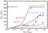 |
Fig. 13 Comparison of the observed RSDs (symbols) and semi-analytical models (lines) from Harsono et al. (2013). The red diamonds indicate the Class 0 sources, blue circles show the Class I sources we have analyzed, and blue triangles show the Class I sources whose parameters were taken from the literatures. TMR1 is indicated by the green circle since the stellar mass is derived from the bolometric luminosity. Different lines show the evolution of RSDs with different initial conditions (cs = 0.26 km s-1 (black and red) and 0.19 km s-1 (blue); Ω = 10-13 Hz (black) and 10-14 Hz (red and blue)), keeping the initial core mass fixed at 1 M⊙. |
A number of RSDs toward other embedded YSOs have been reported in the literature, which are summarized in Table 7. The values are obtained from analysis that included interferometric molecular line observations. Keplerian radii, RK, between 80 and 300 AU are found toward these sources with disk masses in the range 0.004–0.055 M⊙ around 0.2–2.5 M⊙ stars. Most of the observed RSDs are found toward Stage I sources (M⋆ > Menv), while RSDs are claimed toward three Stage 0/I sources. From the sample, large (≥100 AU) RSDs are generally found toward sources where M⋆/Mtot > 0.65 with Mtot = M⋆ + Menv + Mdisk.
How do these disks compare to disk formation models? Semi-analytical disk formation models by Visser et al. (2009), which are based on Terebey et al. (1984) and Cassen & Moosman (1981), predict that >100 AU RSDs are expected by the end of the accretion phase (Menv < Mdisk, see also Young & Evans 2005). The disk sizes depend on the initial envelope temperature or sound speed and the rotation rate. The evolution of RK within these models is shown in Fig. 13 for the same initial conditions as Harsono et al. (2013) with comparable initial rotation rates to those measured by Goodman et al. (1993). Remarkably, the observed RSDs in Stage I fall within the expected sizes from these semi-analytical models. On the other hand, most of the Class 0 disks fall outside of these models. From this comparison, the observed RSDs in Stage I can be well represented by models with Ω = 10-14 Hz and cs = 0.19−0.26 km s-1.
In semi-analytical models, the disk forms as a consequence of angular momentum conservation. However, recent numerical simulations of collapse and disk formation with the presence of magnetic fields do not always form a large RSD (>100 AU). Galli et al. (2006) showed that an RSD does not form in the ideal magnetohydrodynamics (MHD) case due to efficient magnetic breaking (e.g., Galli & Shu 1993; Mellon & Li 2008). The problem can be alleviated if the magnetic field is weak or with the inclusion of non-ideal MHD, although the results with non-ideal MHD are not entirely clear (Mellon & Li 2008, 2009; Dapp & Basu 2010; Krasnopolsky et al. 2011; Li et al. 2011; Braiding & Wardle 2012). Once the RSD forms, it can easily evolve to >400 AU (Dapp et al. 2012; Vorobyov 2010; Joos et al. 2012). The question centers on whether RSDs are already present in the Class 0 phase. This depends on the strength and orientation of the magnetic field, as well as the initial rotation rate of the envelope.
5.2.1. On the magnetic field
The dynamical importance of the magnetic field can be numerically determined through the value of the effective mass-to-flux ratio, λeff, which is the ratio of the gravitational and magnetic energies within the cloud. A value of 1 means that the cloud is strongly magnetized while value of >10 characterizes weakly magnetized clouds. Troland & Crutcher (2008) presented a recent survey of magnetic field strengths toward molecular cloud cores. They find an average λeff ~ 2–3 or an average magnetic field strength of 16 μG, which argues for the importance of magnetic field during the dynamical evolution of pre- and protostellar cores (see also Crutcher 2012).
The magnetic field strength within Taurus is found to vary toward different cores. For example, TMC1A is within the L1534 core whose line of sight magnetic field is weak (<1.2 μG, Crutcher et al. 2010), while the TMC1 dark cloud has considerable magnetic field strength of the order of 9.1 ± 2.2 μG. Since λ is inversely proportional to the magnetic field strength, the λeff toward these two sources are >10 and ~4 around TMC1A and TMC1, respectively. It is interesting to note that a large and massive RSD (R = 100 AU and Mdisk/M⋆ ~ 0.1) is found toward TMC1A, while the RSDs toward both TMC1 and TMR1, which are located closer to the TMC1 dark cloud, are small and less massive. Considering that Mdisk/Menv is lower toward TMC1 and TMR1 than toward TMC1A, this also illustrates that the magnetic field may play an important role in determining the disk properties.
How likely are these disks formed out of weakly magnetized cores? Molecular cloud cores are found to have lower than average magnetic field strength (λeff > 3, Crutcher et al. 2010), than found on cloud scales. On the other hand, the fraction of cores with λeff > 5 is low. Consequently, it is unlikely that TMC1A and other observed RSDs in Stage I all formed out of weakly magnetized cores. Thus, simulations need to be able to form RSDs out of a moderately magnetized core that evolve up to sizes of 100–200 AU by Stage I. In addition, we can argue that the magnetic breaking efficiency drops as the envelope dissipates, which allows the rapid growth of RSDs near the end of the main accretion phase as shown in Fig 13. On the other hand, there may be a low fraction of cores which are weakly magnetized, which facilitate formation of large disks as early as Stage 0 phase (Krumholz et al. 2013; Murillo et al. 2013).
5.2.2. On the large-scale rotation
Another important parameter is the large-scale rotation around these sources, which is a parameter used in both simulations and semi-analytical models. Generally, a cloud rotation rate between 10-14 Hz to a few 10-13 Hz is used in numerical simulations (e.g., Yorke & Bodenheimer 1999; Li et al. 2011). The average rotation rate measured by Goodman et al. (1993) is ~10-14 Hz, which is consistent with the initial rotation rate of the semi-analytical model that best describes a large fraction of the observed RSDs. The time at which Stage I starts within that model is 3 × 10⁵ years. For comparison, around the same computational time, Yorke & Bodenheimer (1999) form a > 500 AU RSD for their low-mass case (J). Similarly, Vorobyov (2010) also found >200 AU RSDs close to the start of the Class II phase. We find no evidence of such large RSDs at similar evolutionary stages in our observations.
Another aspect of the large-scale rotation that is worth investigating is its direction with respect to that of the disk rotation. Models assume that the disk rotation direction is the same as the rotation of its core. To compare the directions, we have used the velocity gradients reported by Caselli et al. (2002) and Goodman et al. (1993) toward the dark cores in Taurus. Velocity gradients are detected toward L1534 (TMC1A), L1536 and TMC-1C, which is located to the North East of TMR1 and TMC1. Table 7 lists the velocity gradients of the RSDs toward the embedded objects and their envelope/core rotation4. It is interesting to note that the large-scale rotation detected around or nearby the RSDs have a different velocity gradient direction. Similar misalignments in rotation have been pointed out by Takakuwa et al. (2012) toward L1551 NE and by Tobin et al. (2013) for L1527. Although the positions of the detected molecular emission in Caselli et al. (2002) do not necessarily coincide with the embedded objects due to chemical effects, the systematic velocities of the cores are similar. Misalignment at 1000 AU scales was also concluded by Brinch et al. (2007) toward L1489 where they found that the Keplerian disk and the rotating envelope are at an angle of 30° with respect to each other. If these objects formed out of these cores in the distant past, then either the collapse process changed the angular momentum of the envelope and, consequently, the disk rotation direction or it affects the angular momentum distribution of nearby cores through feedback. Interestingly, the former may suggest the importance of the non-ideal MHD effect called the Hall effect during disk formation, which can produce counter-rotating disks (Li et al. 2011; Braiding & Wardle 2012).
Finally, the simulations and models above require the initial core to be rotating in order to form RSDs. However, by analyzing the angular momentum distribution of magnetized cores, Dzib et al. (2010) suggested that the NH3 and N2H+ measurements may overestimate the angular momentum by a factor of ~8−10. This poses further problems to disk formation in previous numerical studies of collapse and disk formation. On the other hand, the inclusion of the Hall effect does not require a rotating envelope core to form a rotating structure (e.g., Krasnopolsky et al. 2011; Li et al. 2011). Further studies are required to compare the expected observables from rotating and non-rotating models.
5.3. Disk stability
Self gravitating disks can be important during the early stages of star formation in regulating the accretion process onto the protostar, which can be variable (e.g., Vorobyov 2010). Dunham & Vorobyov (2012) show that such episodic accretion events can reproduce the observed population of YSOs. A self-gravitating disk is expected when Mdisk/Mstar ≥ 0.1 (e.g., Lodato & Rice 2004; Boley et al. 2006; Cossins et al. 2009). However, most of the observed embedded RSDs around Class I sources have disk masses such that Mdisk/Mstar ≤ 0.1. It is unlikely for such disks to become self-gravitating, but they may have been in the past. Interestingly, a few embedded disk seem to be self-gravitating since their Mdisk/Mstar ≥ 0.1 such as toward TMC1A, IRS63, L1527 and NGC1333 IRAS4A2 (See Table 7).
The low fraction of large and massive disks during the embedded phase suggests that disk instabilities may have taken place in the past and limited their current observed numbers (i.e. low fluxes at long baselines). In this scenario, the embedded disks will have a faster evolution and, thus, spend most of their lifetime with small radii. Alternatively, disks experiencing high infall rates from envelope to the disk as expected during the embedded phase may also have higher accretion rates (Harsono et al. 2011). Such a scenario argues for disk instabilities to be present even for Mdisk/M⋆ < 0.1. In both cases, the dominant motion of the compact flattened structure during the embedded phase is infall rather than rotation. There are indeed sources where higher sensitivity and spatial resolution observations such as with Atacama Large Millimeter/submillimeter Array (ALMA) can detect features associated with disk instabilities (e.g., Cossins et al. 2010; Forgan et al. 2012; Douglas et al. 2013).
6. Conclusions
We present spatially and spectrally resolved observations down to a radius of 56 AU around four Class I YSOs in Taurus. The C18O and 13CO 2–1 lines are used to differentiate the infalling rotating envelope from the rotationally supported disk. Analysis of the dust and gas lines were performed directly in uv space to avoid any artefacts introduced during the inversion process. The main results of this paper are:
-
Dust disk sizes and masses can be derived from the continuumby using a power-law spherical envelope model to account forthe large-scale envelope emission. Intensity based disk models(Uniform and Gaussian) give similar disk sizes to each otherwhich are lower by typically 25%–90% than realistic disk mod-els (power-law disk). On the other hand, they give similar diskmasses to more realistic models, which are consistent with thedisk mass derived from the 50 kλ flux point. Inclusion of the envelopein the analysis is important to obtain reliable disk masses. Theobservationally derived masses indicate that there is still a signif-icant envelope present toward three of the four sources: TM1A,TMC1, and TMR1.
-
Three of the four sources (TMC1, L1536, TMC1A) host embedded rotationally supported disks (RSDs) derived from line data. By fitting velocity profiles (υ ∝ r-0.5 or ∝ r-1.0) to the red- and blue-shifted peaks, the RSDs are found to have outer radii of ~80–100 AU. In addition, the large-scale structure (>100 AU) is dominated by the infalling rotating envelope (υ ∝ r-1). The derived stellar masses of these sources are of order 0.4–0.8 M⊙, consistent with previous values. Consequently, these objects are indeed Stage I young stellar objects with M⋆/(Menv + Mdisk + M⋆) > 0.7.
-
Disk radii derived from the power-law dust disk models toward TMC1 and TMC1A are consistent with sizes of their RSDs. However, the dust disk radii toward TMR1 and L1536 are not the same as the extent of their RSDs. Thus, we emphasize that spatially and spectrally resolved gas lines observations are required to study the nature of flattened structures toward embedded YSOs.
-
Semi-analytical models with Ω = 10-14 Hz and cs = 0.19−0.26 km s-1describe most of the observed RSDs in Stage I. The observed RSDs argue for inefficient magnetic breaking near the end of the main accretion phase (M⋆/Mtot > 0.65). More theoretical studies are needed to understand how and when RSDs form under such conditions.
-
Comparison between disk masses derived from the continuum and C18O integrated line intensities (Table 6) suggests that relatively little of CO is frozen out within the embedded disk.
Online material
Appendix A: Observational data
The observational log can be found in Table A.1 and the channel maps of all the observed lines toward the four sources are shown in Figs. A.1–A.6.
Observational log.
Appendix B: Large-scale structure
The parameters of the large-scale envelope structure used to estimate the continuum emission at short baselines are in Table B.1.
1D spherical envelope parameters as published by Kristensen et al. (2012).
Appendix C: WideX data
Spectra toward all sources integrated within a 3″ box around their continuum positions are shown in Fig. C.1. The integrated flux density maps toward C18O, SO 56−45 and SO2 11111−100010 (221.96521 GHz) are shown in Fig. C.3. The SO emission toward all sources is much more extended compared to the C18O emission, while the SO2 emission is compact.
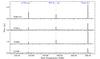 |
Fig. C.1 Integrated flux of C18O J = 2–1, SO 56–45 and 13CO J = 2–1 within a 3″ box around each source in the WideX spectra. |
 |
Fig. C.2 Integrated flux within a 1″ box around each source in the WideX spectra between 220.7–222.1 GHz. |
 |
Fig. C.3 Moment 0 maps of C18O J = 2–1, SO 56–45 and SO2 11111−100010 toward all sources from the WideX data. The contours are drawn at 10% of the peak starting at 3σ. Green star indicates the continuum position and black ellipses show the synthesized beams. |
Appendix D: L1536
Figure D.1 shows the 12CO J = 3–2 spectral map obtained with JCMT, where there is no indication of classical bipolar outflows are present.
 |
Fig. D.1 12CO J = 3–2 spectral map obtained with the JCMT from –5 km s-1 to 15 km s-1 and intensities from –0.5 K to 3.5 K. The vertical dotted lines show 0, 5.2, and 10 km s-1 for guidance. |
Recent 12CO 3–2 observations with the JCMT do not show any indication of a bipolar outflow from this source, see Appendix D.
We note that our observed visibilities (Fig. 7) are a factor of 3 higher than that reported by Eisner (2012) for TMC1A at 50 kλ.
The direction is in degrees East of North and increasing υlsr (blue to red) to be consistent with Caselli et al. (2002) and Goodman et al. (1993).
Acknowledgments
We thank the anonymous referee for the constructive comments. We are grateful to the IRAM staff, in particular to Chin-Shin Chang, Tessel van der Laan and Jérôme Pety, for their help with the observations, reduction and modelling of the data. We thank Umut Yıldız for reducing the single-dish data and making them available. This work is supported by the Netherlands Research School for Astronomy (NOVA) and by the Space Research Organization Netherlands (SRON). Astrochemistry in Leiden is supported by the Netherlands Research School for Astronomy (NOVA), by a Spinoza grant and grant 614.001.008 from the Netherlands Organisation for Scientific Research (NWO), and by the European Community’s Seventh Framework Programme FP7/2007–2013 under grant agreement 238258 (LASSIE). This research was supported by a Lundbeck Foundation Group Leader Fellowship to Jes Jørgensen. Research at Centre for Star and Planet Formation is funded by the Danish National Research Foundation and the University of Copenhagen’s programme of excellence. This research used the facilities of the Canadian Astronomy Data Centre operated by the National Research Council of Canada with the support of the Canadian Space Agency.
References
- Aikawa, Y., Wakelam, V., Garrod, R. T., & Herbst, E. 2008, ApJ, 674, 984 [NASA ADS] [CrossRef] [Google Scholar]
- Aikawa, Y., Furuya, K., Wakelam, V., et al. 2011, in IAU Symp. 280, eds. J. Cernicharo & R. Bachiller, 33 [Google Scholar]
- Andre, P., Ward-Thompson, D., & Barsony, M. 1993, ApJ, 406, 122 [NASA ADS] [CrossRef] [Google Scholar]
- Berger, J. P., & Segransan, D. 2007, New A Rev., 51, 576 [NASA ADS] [CrossRef] [Google Scholar]
- Bodenheimer, P. 1995, ARA&A, 33, 199 [NASA ADS] [CrossRef] [Google Scholar]
- Boley, A. C., Mejía, A. C., Durisen, R. H., et al. 2006, ApJ, 651, 517 [NASA ADS] [CrossRef] [Google Scholar]
- Braiding, C. R., & Wardle, M. 2012, MNRAS, 422, 261 [NASA ADS] [CrossRef] [Google Scholar]
- Brinch, C., & Jørgensen, J. K. 2013, A&A, 559, A82 [NASA ADS] [CrossRef] [EDP Sciences] [Google Scholar]
- Brinch, C., Crapsi, A., Jørgensen, J. K., Hogerheijde, M. R., & Hill, T. 2007, A&A, 475, 915 [Google Scholar]
- Brinch, C., Hogerheijde, M. R., & Richling, S. 2008, A&A, 489, 607 [NASA ADS] [CrossRef] [EDP Sciences] [Google Scholar]
- Brown, D. W., & Chandler, C. J. 1999, MNRAS, 303, 855 [NASA ADS] [CrossRef] [Google Scholar]
- Cabrit, S., Guilloteau, S., Andre, P., et al. 1996, A&A, 305, 527 [NASA ADS] [Google Scholar]
- Caselli, P., Benson, P. J., Myers, P. C., & Tafalla, M. 2002, ApJ, 572, 238 [NASA ADS] [CrossRef] [Google Scholar]
- Cassen, P., & Moosman, A. 1981, Icarus, 48, 353 [NASA ADS] [CrossRef] [Google Scholar]
- Chiang, H.-F., Looney, L. W., Tassis, K., Mundy, L. G., & Mouschovias, T. C. 2008, ApJ, 680, 474 [NASA ADS] [CrossRef] [Google Scholar]
- Chiang, H.-F., Looney, L. W., & Tobin, J. J. 2012, ApJ, 756, 168 [NASA ADS] [CrossRef] [Google Scholar]
- Choi, M., Tatematsu, K., & Kang, M. 2010, ApJ, 723, L34 [NASA ADS] [CrossRef] [Google Scholar]
- Cossins, P., Lodato, G., & Clarke, C. J. 2009, MNRAS, 393, 1157 [Google Scholar]
- Cossins, P., Lodato, G., & Testi, L. 2010, MNRAS, 407, 181 [NASA ADS] [CrossRef] [Google Scholar]
- Crapsi, A., van Dishoeck, E. F., Hogerheijde, M. R., Pontoppidan, K. M., & Dullemond, C. P. 2008, A&A, 486, 245 [NASA ADS] [CrossRef] [EDP Sciences] [Google Scholar]
- Crutcher, R. M. 2012, ARA&A, 50, 29 [NASA ADS] [CrossRef] [Google Scholar]
- Crutcher, R. M., Hakobian, N., & Troland, T. H. 2010, MNRAS, 402, L64 [NASA ADS] [Google Scholar]
- Dapp, W. B., & Basu, S. 2010, A&A, 521, L56 [NASA ADS] [CrossRef] [EDP Sciences] [Google Scholar]
- Dapp, W. B., Basu, S., & Kunz, M. W. 2012, A&A, 541, A35 [NASA ADS] [CrossRef] [EDP Sciences] [Google Scholar]
- Di Francesco, J., Johnstone, D., Kirk, H., MacKenzie, T., & Ledwosinska, E. 2008, ApJS, 175, 277 [NASA ADS] [CrossRef] [Google Scholar]
- Douglas, T. A., Caselli, P., Ilee, J. D., et al. 2013, MNRAS, 433, 2064 [NASA ADS] [CrossRef] [Google Scholar]
- Dunham, M. M., & Vorobyov, E. I. 2012, ApJ, 747, 52 [NASA ADS] [CrossRef] [Google Scholar]
- Dunham, M. M., Evans, II, N. J., Terebey, S., Dullemond, C. P., & Young, C. H. 2010, ApJ, 710, 470 [NASA ADS] [CrossRef] [Google Scholar]
- Dutrey, A., Guilloteau, S., & Ho, P. 2007, in Protostars and Planets V, B. Reipurth, eds. D. Jewitt, & K. Keil (Tucson: University of Arizona Press), 951, 495 [Google Scholar]
- Dzib, S., Loinard, L., Mioduszewski, A. J., et al. 2010, ApJ, 718, 610 [NASA ADS] [CrossRef] [Google Scholar]
- Eisner, J. A. 2012, ApJ, 755, 23 [NASA ADS] [CrossRef] [Google Scholar]
- Eisner, J. A., Hillenbrand, L. A., Carpenter, J. M., & Wolf, S. 2005, ApJ, 635, 396 [NASA ADS] [CrossRef] [Google Scholar]
- Enoch, M. L., Corder, S., Dunham, M. M., & Duchêne, G. 2009, ApJ, 707, 103 [NASA ADS] [CrossRef] [Google Scholar]
- Enoch, M. L., Corder, S., Duchêne, G., et al. 2011, ApJS, 195, 21 [NASA ADS] [CrossRef] [Google Scholar]
- Forgan, D., Armitage, P. J., & Simon, J. B. 2012, MNRAS, 426, 2419 [NASA ADS] [CrossRef] [Google Scholar]
- Furlan, E., McClure, M., Calvet, N., et al. 2008, ApJS, 176, 184 [NASA ADS] [CrossRef] [Google Scholar]
- Galli, D., & Shu, F. H. 1993, ApJ, 417, 220 [NASA ADS] [CrossRef] [Google Scholar]
- Galli, D., Lizano, S., Shu, F. H., & Allen, A. 2006, ApJ, 647, 374 [NASA ADS] [CrossRef] [Google Scholar]
- Goodman, A. A., Benson, P. J., Fuller, G. A., & Myers, P. C. 1993, ApJ, 406, 528 [NASA ADS] [CrossRef] [Google Scholar]
- Gramajo, L. V., Whitney, B. A., Kenyon, S. J., Gómez, M., & Merrill, K. M. 2007, AJ, 133, 1911 [NASA ADS] [CrossRef] [Google Scholar]
- Gramajo, L. V., Whitney, B. A., Gómez, M., & Robitaille, T. P. 2010, AJ, 139, 2504 [NASA ADS] [CrossRef] [Google Scholar]
- Harsono, D., Alexander, R. D., & Levin, Y. 2011, MNRAS, 413, 423 [NASA ADS] [CrossRef] [Google Scholar]
- Harsono, D., Visser, R., Bruderer, S., van Dishoeck, E. F., & Kristensen, L. E. 2013, A&A, 555, A45 [NASA ADS] [CrossRef] [EDP Sciences] [Google Scholar]
- Hayashi, M., Ohashi, N., & Miyama, S. M. 1993, ApJ, 418, L71 [NASA ADS] [CrossRef] [Google Scholar]
- Hogerheijde, M. R., van Dishoeck, E. F., Blake, G. A., & van Langevelde, H. J. 1998, ApJ, 502, 315 [NASA ADS] [CrossRef] [PubMed] [Google Scholar]
- Ivezic, Z., & Elitzur, M. 1997, MNRAS, 287, 799 [NASA ADS] [CrossRef] [Google Scholar]
- Joos, M., Hennebelle, P., & Ciardi, A. 2012, A&A, 543, A128 [NASA ADS] [CrossRef] [EDP Sciences] [Google Scholar]
- Jørgensen, J. K., Schöier, F. L., & van Dishoeck, E. F. 2002, A&A, 389, 908 [NASA ADS] [CrossRef] [EDP Sciences] [Google Scholar]
- Jørgensen, J. K., Bourke, T. L., Myers, P. C., et al. 2005, ApJ, 632, 973 [NASA ADS] [CrossRef] [Google Scholar]
- Jørgensen, J. K., Bourke, T. L., Myers, P. C., et al. 2007, ApJ, 659, 479 [NASA ADS] [CrossRef] [Google Scholar]
- Jørgensen, J. K., van Dishoeck, E. F., Visser, R., et al. 2009, A&A, 507, 861 [NASA ADS] [CrossRef] [EDP Sciences] [Google Scholar]
- Keene, J., & Masson, C. R. 1990, ApJ, 355, 635 [NASA ADS] [CrossRef] [Google Scholar]
- Krasnopolsky, R., Li, Z.-Y., & Shang, H. 2011, ApJ, 733, 54 [NASA ADS] [CrossRef] [Google Scholar]
- Kristensen, L. E., van Dishoeck, E. F., Bergin, E. A., et al. 2012, A&A, 542, A8 [NASA ADS] [CrossRef] [EDP Sciences] [Google Scholar]
- Krumholz, M. R., Crutcher, R. M., & Hull, C. L. H. 2013, ApJ, 767, L11 [NASA ADS] [CrossRef] [Google Scholar]
- Lada, C. J., & Wilking, B. A. 1984, ApJ, 287, 610 [NASA ADS] [CrossRef] [Google Scholar]
- Lay, O. P., Carlstrom, J. E., Hills, R. E., & Phillips, T. G. 1994, ApJ, 434, L75 [NASA ADS] [CrossRef] [Google Scholar]
- Lay, O. P., Carlstrom, J. E., & Hills, R. E. 1997, ApJ, 489, 917 [NASA ADS] [CrossRef] [Google Scholar]
- Lee, C.-F. 2010, ApJ, 725, 712 [NASA ADS] [CrossRef] [Google Scholar]
- Lee, C.-F. 2011, ApJ, 741, 62 [NASA ADS] [CrossRef] [Google Scholar]
- Li, Z.-Y., Krasnopolsky, R., & Shang, H. 2011, ApJ, 738, 180 [NASA ADS] [CrossRef] [Google Scholar]
- Lin, D. N. C., Hayashi, M., Bell, K. R., & Ohashi, N. 1994, ApJ, 435, 821 [NASA ADS] [CrossRef] [Google Scholar]
- Lindberg, J. E., Jørgensen, J. K., Brinch, C., et al. 2014, A&A, submitted [Google Scholar]
- Lodato, G., & Rice, W. K. M. 2004, MNRAS, 351, 630 [Google Scholar]
- Lommen, D., Jørgensen, J. K., van Dishoeck, E. F., & Crapsi, A. 2008, A&A, 481, 141 [NASA ADS] [CrossRef] [EDP Sciences] [Google Scholar]
- Looney, L. W., Mundy, L. G., & Welch, W. J. 2003, ApJ, 592, 255 [NASA ADS] [CrossRef] [Google Scholar]
- Looney, L. W., Tobin, J. J., & Kwon, W. 2007, ApJ, 670, L131 [NASA ADS] [CrossRef] [Google Scholar]
- Malbet, F., Lachaume, R., Berger, J.-P., et al. 2005, A&A, 437, 627 [Google Scholar]
- Mellon, R. R., & Li, Z.-Y. 2008, ApJ, 681, 1356 [NASA ADS] [CrossRef] [Google Scholar]
- Mellon, R. R., & Li, Z.-Y. 2009, ApJ, 698, 922 [NASA ADS] [CrossRef] [Google Scholar]
- Momose, M., Ohashi, N., Kawabe, R., Nakano, T., & Hayashi, M. 1998, ApJ, 504, 314 [NASA ADS] [CrossRef] [Google Scholar]
- Motte, F., & André, P. 2001, A&A, 365, 440 [NASA ADS] [CrossRef] [EDP Sciences] [Google Scholar]
- Mundy, L. G., Looney, L. W., Erickson, W., et al. 1996, ApJ, 464, L169 [NASA ADS] [CrossRef] [Google Scholar]
- Murillo, N. M., & Lai, S.-P. 2013, ApJ, 764, L15 [Google Scholar]
- Murillo, N. M., Lai, S.-P., Bruderer, S., Harsono, D., & van Dishoeck, E. F. 2013, A&A, 560, A103 [NASA ADS] [CrossRef] [EDP Sciences] [Google Scholar]
- Ohashi, N., Hayashi, M., Ho, P. T. P., & Momose, M. 1997a, ApJ, 475, 211 [Google Scholar]
- Ohashi, N., Hayashi, M., Ho, P. T. P., et al. 1997b, ApJ, 488, 317 [NASA ADS] [CrossRef] [Google Scholar]
- Ossenkopf, V., & Henning, T. 1994, A&A, 291, 943 [NASA ADS] [Google Scholar]
- Robitaille, T. P., Whitney, B. A., Indebetouw, R., Wood, K., & Denzmore, P. 2006, ApJS, 167, 256 [NASA ADS] [CrossRef] [Google Scholar]
- Sargent, A. I., & Beckwith, S. 1987, ApJ, 323, 294 [NASA ADS] [CrossRef] [Google Scholar]
- Scoville, N. Z., Sargent, A. I., Sanders, D. B., et al. 1986, ApJ, 303, 416 [NASA ADS] [CrossRef] [Google Scholar]
- Takakuwa, S., Saito, M., Lim, J., et al. 2012, ApJ, 754, 52 [NASA ADS] [CrossRef] [Google Scholar]
- Terebey, S., Shu, F. H., & Cassen, P. 1984, ApJ, 286, 529 [NASA ADS] [CrossRef] [Google Scholar]
- Tobin, J. J., Hartmann, L., Looney, L. W., & Chiang, H.-F. 2010, ApJ, 712, 1010 [NASA ADS] [CrossRef] [Google Scholar]
- Tobin, J. J., Hartmann, L., Chiang, H.-F., et al. 2012, Nature, 492, 83 [NASA ADS] [CrossRef] [PubMed] [Google Scholar]
- Tobin, J. J., Hartmann, L., Chiang, H.-F., et al. 2013, ApJ, 771, 48 [NASA ADS] [CrossRef] [Google Scholar]
- Troland, T. H., & Crutcher, R. M. 2008, ApJ, 680, 457 [NASA ADS] [CrossRef] [Google Scholar]
- Ulrich, R. K. 1976, ApJ, 210, 377 [NASA ADS] [CrossRef] [Google Scholar]
- Visser, R., van Dishoeck, E. F., Doty, S. D., & Dullemond, C. P. 2009, A&A, 495, 881 [NASA ADS] [CrossRef] [EDP Sciences] [Google Scholar]
- Visser, R., Doty, S. D., & van Dishoeck, E. F. 2011, A&A, 534, A132 [NASA ADS] [CrossRef] [EDP Sciences] [Google Scholar]
- Vorobyov, E. I. 2010, ApJ, 723, 1294 [NASA ADS] [CrossRef] [Google Scholar]
- Whitney, B. A., Wood, K., Bjorkman, J. E., & Wolff, M. J. 2003, ApJ, 591, 1049 [Google Scholar]
- Williams, J. P., & Cieza, L. A. 2011, ARA&A, 49, 67 [NASA ADS] [CrossRef] [Google Scholar]
- Wilson, T. L., & Rood, R. 1994, ARA&A, 32, 191 [NASA ADS] [CrossRef] [Google Scholar]
- Yen, H.-W., Takakuwa, S., Ohashi, N., & Ho, P. T. P. 2013, ApJ, 772, 22 [NASA ADS] [CrossRef] [Google Scholar]
- Yıldız, U. A., Kristensen, L. E., van Dishoeck, E. F., et al. 2013, A&A, 556, A89 [NASA ADS] [CrossRef] [EDP Sciences] [Google Scholar]
- Yorke, H. W., & Bodenheimer, P. 1999, ApJ, 525, 330 [NASA ADS] [CrossRef] [Google Scholar]
- Young, C. H., & Evans, II, N. J. 2005, ApJ, 627, 293 [NASA ADS] [CrossRef] [Google Scholar]
- Young, C. H., Shirley, Y. L., Evans, II, N. J., & Rawlings, J. M. C. 2003, ApJS, 145, 111 [NASA ADS] [CrossRef] [Google Scholar]
All Tables
1.36 mm continuum properties from elliptical Gaussian fits and derived disk and envelope masses (within 15′′) from fluxes.
13CO and C18O 2–1 integrated flux densities [Jy km s-1] within a 5″ box around continuum position.
Disk sizes and masses derived from continuum visibilities modelling using uniform, Gaussian and power-law disk models.
Derived disk sizes and stellar masses from the break radius in the uv-space PV diagrams corrected for inclination.
All Figures
|
Fig. 1 1.36 mm uniform weighted continuum maps toward TMC1A (I4365+2535, top left), TMC1 (I4381+2540, top right), TMR1 (I4361+2547, bottom left), and L1536 (I4295+2251, bottom right). The contours start from 10σ up to 80σ by 10σ. The peak flux densities per beam are 11 mJy, 42 mJy, 23 mJy and 128 mJy for TMC1, TMR1, L1536 and TMC1A, respectively. The red circles indicate the best-fit source-position assuming elliptical Gaussian while the black ellipses show the synthesized beams. The arrows indicate the outflow direction. The RMS is given in Table 1. The dashed blue lines indicate the negative contours starting at 3σ. |
| In the text | |
|
Fig. 2 Zoom of the continuum image toward L1536. Both of the line and color contours are drawn at 10% of the peak starting from 4σ up to the peak intensity of 23 mJy beam-1, while the synthesized beam is indicated by the black ellipse in the bottom right corner. |
| In the text | |
|
Fig. 3 Left: 13CO (top) and C18O 2–1 (bottom) spectra integrated within a 1″ box around the continuum position. Right: single-dish spectra of 13CO 3–2 (except for L1536, which is 13CO 2–1) and C18O 2–1. The vertical red dotted lines indicate the systemic velocities of each source derived from single dish C18O and C17O data (Yıldız et al. 2013). The horizontal blue lines indicate the spectral σrms. |
| In the text | |
|
Fig. 4 13CO (left) and C18O (right) 2–1 channel maps within the inner 10″ toward TMC1A. The velocities in km s-1 are indicated at the top left in each panel. The contours are drawn at every 3σ starting from 5σ where σ = 12 mJy km s-1 for 13CO and 10 mJy km s-1 for C18O. |
| In the text | |
|
Fig. 5 13CO (top) and C18O (bottom) moment zero maps. The contours are drawn at intervals of 10% of the peak starting from 5σ. The continuum position is indicated by the green stars and the arrows show the direction of the red and blue-shifted outflow components taken from the literature (TMC1: 0°; TMR1: 165°; TMC1A: 155°; L1536: None Ohashi et al. 1997a; Hogerheijde et al. 1998; Brown & Chandler 1999). The bottom row show C18O integrated flux maps from the velocity unresolved spectra (typically 1–2 channels) taken within the WideX with contours of 10% of the peak starting from 3σ (~30 mJy beam-1 km s-1). The zero moment maps are obtained by integrating over the velocity ranges [υmin,υmax] = [−3, 11] , [−1, 11] , [−2, 12] , [−2, 12] for TMC1A, TMC1, TMR1, and L1536, respectively. |
| In the text | |
|
Fig. 6 13CO and C18O moment 1 maps within the inner 5″ (700 AU). The solid line indicate the 100 AU scale and the ellipses show the synthesized beams. The gray crosses show the continuum positions. |
| In the text | |
|
Fig. 7 Circularly averaged 1.36 mm visibility amplitudes as function of projected baselines in kλ. The black circles are from this work while the red circles are from previous SMA observations at 1.1 mm (Jørgensen et al. 2009) scaled to 1.36 mm with α = 2.5. The error bars indicate the statistical errors of each bin. The blue line is the simulated continuum emission of the spherical envelope model from Kristensen et al. (2012) sampled using the observed uv points. An arrow in the first panel shows an example of the continuum excess toward TMC1A. Solid squares are the 1.36 mm single-dish flux. The zero-expectation level given in dotted line is the expected amplitude due to noise in the absence of source emission. |
| In the text | |
|
Fig. 8 Left: normalized intensity profiles for the three different continuum models: Uniform disk (top), Gaussian Disk (middle), and power-law disk (bottom). Right: normalized visibilities as function of uv radius. For comparison, the L1536 binned data are shown in gray circles. |
| In the text | |
|
Fig. 9 13CO position velocity diagrams along the direction perpendicular to the outflow: TMC1A (top left), TMC1 (top right), TMR1 (bottom left), and L1536 (bottom right). The color contours start from 3σ and increase by 1σ while the black line contours are drawn at 5σ, 8σ, 11σ, and so on up to the peak intensity. The black solid curves show the best-fit Keplerian curves, while the dashed lines indicate the r-1 curves. For TMC1A and TMC1 (top row), the blue solid line presents a 0.4 M⊙ Keplerian curve. |
| In the text | |
|
Fig. 10 C18O uv-space PV diagrams toward TMC1A with PA = 55°,65° and υlsr = 6.6,6.4 km s-1. The solid lines are the r-0.5 curves and dashed lines are the r-1 curves. The red and blue colors indicate the red- and blue-shifted components, respectively. Gray points show the rest of the peaks that were not included in the fitting. |
| In the text | |
|
Fig. 11 13CO uv-space PV diagrams toward all sources with the best fit profiles superposed in black lines (except for L1536). The red lines indicate a υ ∝ r-1 as comparison. Gray points show the peaks that were not included in the fitting. |
| In the text | |
|
Fig. 12 C18O uv-space PV diagrams toward TMC1 derived from the emission peaks. The solid line indicates the best-fit power-law slope to the peaks between 1.3–1.9 km s-1. The vertical blue dotted lines indicate the 150 AU radius. The red and blue colors indicate the red- and blue-shifted components, respectively. |
| In the text | |
|
Fig. 13 Comparison of the observed RSDs (symbols) and semi-analytical models (lines) from Harsono et al. (2013). The red diamonds indicate the Class 0 sources, blue circles show the Class I sources we have analyzed, and blue triangles show the Class I sources whose parameters were taken from the literatures. TMR1 is indicated by the green circle since the stellar mass is derived from the bolometric luminosity. Different lines show the evolution of RSDs with different initial conditions (cs = 0.26 km s-1 (black and red) and 0.19 km s-1 (blue); Ω = 10-13 Hz (black) and 10-14 Hz (red and blue)), keeping the initial core mass fixed at 1 M⊙. |
| In the text | |
 |
Fig. A.1 13CO 2–1 channel maps similar to Fig. 4 toward TMC1. |
| In the text | |
 |
Fig. A.2 C18O 2–1 channel maps similar to Fig. 4 toward TMC1. |
| In the text | |
 |
Fig. A.3 13CO 2–1 channel maps similar to Fig. 4 toward TMR1. |
| In the text | |
 |
Fig. A.4 C18O 2–1 channel maps similar to Fig. 4 toward TMR1. |
| In the text | |
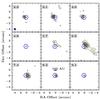 |
Fig. A.5 13CO 2–1 channel maps similar to Fig. 4 toward L1536. |
| In the text | |
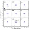 |
Fig. A.6 C18O 2–1 channel maps similar to Fig. 4 toward L1536. |
| In the text | |
|
Fig. C.1 Integrated flux of C18O J = 2–1, SO 56–45 and 13CO J = 2–1 within a 3″ box around each source in the WideX spectra. |
| In the text | |
|
Fig. C.2 Integrated flux within a 1″ box around each source in the WideX spectra between 220.7–222.1 GHz. |
| In the text | |
|
Fig. C.3 Moment 0 maps of C18O J = 2–1, SO 56–45 and SO2 11111−100010 toward all sources from the WideX data. The contours are drawn at 10% of the peak starting at 3σ. Green star indicates the continuum position and black ellipses show the synthesized beams. |
| In the text | |
|
Fig. D.1 12CO J = 3–2 spectral map obtained with the JCMT from –5 km s-1 to 15 km s-1 and intensities from –0.5 K to 3.5 K. The vertical dotted lines show 0, 5.2, and 10 km s-1 for guidance. |
| In the text | |
Current usage metrics show cumulative count of Article Views (full-text article views including HTML views, PDF and ePub downloads, according to the available data) and Abstracts Views on Vision4Press platform.
Data correspond to usage on the plateform after 2015. The current usage metrics is available 48-96 hours after online publication and is updated daily on week days.
Initial download of the metrics may take a while.