| Issue |
A&A
Volume 559, November 2013
|
|
|---|---|---|
| Article Number | A37 | |
| Number of page(s) | 10 | |
| Section | Cosmology (including clusters of galaxies) | |
| DOI | https://doi.org/10.1051/0004-6361/201321882 | |
| Published online | 01 November 2013 | |
Mass-sheet degeneracy, power-law models and external convergence: Impact on the determination of the Hubble constant from gravitational lensing
Argelander-Institut für Astronomie, Universität Bonn, Auf dem Hügel 71, 53121 Bonn, Germany
e-mail: peter@astro.uni-bonn.de
Received: 13 May 2013
Accepted: 12 September 2013
The light travel time differences in strong gravitational lensing systems allows an independent determination of the Hubble constant. This method has been successfully applied to several lens systems. The formally most precise measurements are, however, in tension with the recent determination of H0 from the Planck satellite for a spatially flat six-parameters ΛCDM cosmology. We reconsider the uncertainties of the method, concerning the mass profile of the lens galaxies, and show that the formal precision relies on the assumption that the mass profile is a perfect power law. Simple analytical arguments and numerical experiments reveal that mass-sheet like transformations yield significant freedom in choosing the mass profile, even when exquisite Einstein rings are observed. Furthermore, the characterization of the environment of the lens does not break that degeneracy which is not physically linked to extrinsic convergence. We present an illustrative example where the multiple imaging properties of a composite (baryons + dark matter) lens can be extremely well reproduced by a power-law model having the same velocity dispersion, but with predictions for the Hubble constant that deviate by ~20%. Hence we conclude that the impact of degeneracies between parametrized models have been underestimated in current H0 measurements from lensing, and need to be carefully reconsidered.
Key words: cosmological parameters / gravitational lensing: strong
© ESO, 2013
1. Introduction
Half a century ago, Sjur Refsdal (1964) pointed out that a gravitational lens system can be used for determining the Hubble constant H0, provided that the difference in light-travel time along the different light rays can be measured. The identification of active galactic nuclei as variable, distant extragalactic sources, as well as the discovery of gravitational lens systems allowed this idea to be turned into a target of research. Immediately after the discovery of the first gravitational lens system (Walsh et al. 1979), the flux variations of its two compact components were monitored, and a firm measurement of the time delay was obtained in 1997 (Kundic et al. 1997), with sub-percent accuracy. Since then, the time delays in about 20 other lens systems have been measured (see e.g. Paraficz & Hjorth 2010; Courbin et al. 2011; Eulaers & Magain 2011; Tewes et al. 2013; Fohlmeister et al. 2013; Eulaers et al. 2013, for a compilation and recent measurements).
To transform a measured time delay into an estimate of the Hubble constant, the mass distribution in the lens system needs to be determined with sufficient accuracy. Since our physical understanding of the mass distribution in the inner parts of galaxies is insufficient, parametrized mass models are employed whose parameters are fixed by the observational constraints, like the angular positions of compact images of the source, morphology of extended image components, or sometimes flux ratios. Reassuringly, “simple” parametrized mass models yield an accurate description of the image morphologies in most lens systems, without the need for more complex matter distributions. These models are further constrained by additional information, such as measurements of the stellar velocity dispersion in the lens galaxy. As a result, one obtains a good model (in the sense that it fits the data) for the mass distribution in the inner part (i.e. within a few effective radii) of lens galaxies, which together with time delay measurements is used to estimate H0.
An excellent account of the early history of H0 measurements from lensing can be found in Kochanek et al. (2004). In particular, estimated values of H0 varied substantially from system to system, and even different analyses for the same system sometimes gave substantially differing values. This can be traced back to the non-uniqueness of the mass model. Since a typical gravitational lens system has two or four images, the number of observational constraints on the mass model is small, and there is more than one density profile which can reproduce the observed image positions. Different values of H0 result if one assumes either an isothermal profile (one where the volume mass density behaves like ρ ∝ r-2) or a mass profile which follows closely the projected brightness profile. These two different model assumptions lead to different slopes of the density in the region where the strong lensing constraints are available, and this slope affects the product of time delay and Hubble constant, τ = H0 Δt (Kochanek 2002). Indeed, Falco et al. (1985) pointed out the so-called mass-sheet degeneracy (MSD), which provides a transformation of the mass profile which leaves all lensing observables exactly invariant, except H0 Δt. The mass-sheet degeneracy and families of degeneracies have been discussed in Gorenstein et al. (1988); Saha (2000); Wucknitz (2002); Liesenborgs & De Rijcke (2012). The MSD is the basic reason why the estimated values of H0 from lensing have been so different.
More recently, Suyu et al. (2010; 2013a) studied two four-image lens systems in great detail, making use of multi-color images from the Hubble Space Telescope and spectroscopy of the lens galaxies in these systems. Together with the measured time delays, they obtained a value of H0 = 70.6 ± 3.1 km s-1 Mpc-1 for B1608+656 and  for RXJ1131–1231. Motivated by the recent results from the Planck satellite (Planck Collaboration 2013), which yield a value of H0 = 67.3 ± 1.2 km s-1 Mpc-1 for a spatially flat ΛCDM cosmology, we reconsider some issues related to the determination of the Hubble constant from gravitational lensing. In Sect. 2, we briefly review the basics of the MSD and its consequences. We then discuss in Sect. 3 the uniqueness of power-law mass models, which have been widely employed for strong lens modeling, and the impact of possible deviations from a power law. More complicated (though arguably more realistic) mass profiles are considered in Sect. 4. We show that those models are (almost) degenerate with global power-law profiles leading to quite different values of τ. Section 5 considers the original interpretation of the mass-sheet degeneracy, as an additional surface mass density related to a galaxy cluster, or some overdensity along the line-of-sight. We will argue that the mass-sheet degeneracy is in general not broken by observing the environmental (or “external”) convergence. We briefly conclude in Sect. 6.
2. The mass-sheet degeneracy
We use standard gravitational lensing notation (Schneider et al. 1992); in particular, κ(θ) is the dimensionless surface mass density (or convergence) at angular position θ, ψ(θ) the deflection potential, satisfying the two-dimensional Poisson equation ∇2ψ = 2κ, and α(θ) = ∇ψ is the scaled deflection angle. The lens equation β = θ − α(θ) relates the observed angular position θ on the sky to the true intrinsic position β in the absence of light deflection. The Jacobian matrix of the lens mapping is denoted by  , and the (signed) magnification of an image of an infinitesimally small source is
  . Critical curves in the lens plane, i.e., curves of formally infinite magnification, are characterized by
  .
.
2.1. The mass-sheet transformation
As shown by Falco et al. (1985), the mass distribution κ(θ) and each of the distributions  (1)together with an (in most cases unobservable; see below) isotropic scaling of the source plane coordinates β → λ β, yields exactly the same dimensionless observables, i.e., image positions, image shapes, magnification ratios, etc. This is called the mass-sheet degeneracy (MSD). In other words, from the observed image positions and flux ratios, one cannot distinguish between the original κ and any of the mass distributions in (1). As shown by Schneider & Seitz (1995), also weak gravitational lensing cannot break the MSD, since image shapes are unaffected. However, the product of the time delay and the Hubble constant is affected, H0 Δt → λ H0 Δt, but leaving time delay ratios again invariant.
2.2. Breaking the mass-sheet degeneracy
The mass-sheet transformation (MST) leaves the critical curves invariant, also the curves on which κ = 1. Furthermore, it leaves the shapes of the isodensity contours invariant, just the value of κ on these contours changes according to (1).
As is clear from the transformation of H0 Δt, in order to get a reliable estimate of the Hubble constant from gravitational lensing, one first needs to break the MSD. Several ways have been suggested in the literature. Some of these make use of the fact that the MST (1) affects the magnification, μ → μ/λ2, hence if the magnification can be estimated, the value of λ can be constrained (this magnification corresponds to the aforementioned isotropic scaling of the source plane coordinates). For AGN as sources, which have a very broad distribution of intrinsic luminosities, this cannot be easily accomplished. Whereas Bauer et al. (2012) have shown that the correlation between AGN variability properties and luminosity can be used as a tool for estimating source luminosities, and hence lensing magnification, the scatter of the variability–luminosity relation is large and can only be employed in a statistical way.
Another possibility to break the MSD in strong lensing systems is based on independent mass estimates of the lens. Combining lensing measurements with spectroscopy of the lens galaxy, the MSD can be broken. The use of velocity dispersion measurements in estimates of H0 with the time-delay technique started with the modeling of Q0957+561 by Grogin & Narayan (1996). It was later refined by Romanowsky & Kochanek (1999) who suggested to use higher-order moments of the stellar velocity distribution. For early-type galaxies (most lenses are of that type), the stellar velocity dispersion yields an estimate of the mass inside the effective radius of the lens, which together with the precise (and unaffected by the MST) determination of the mass inside the Einstein radius of the lens allows one to determine the mean slope γ′ of the mass profile between the effective radius and the Einstein radius. The Lens Structure and Dynamics Survey (LSD) initiated the use of velocity dispersion to derive the average slope of the mass density profile of lensing galaxies (Treu & Koopmans 2002). Since then, many more systems have been studied (Rusin & Kochanek 2005; Koopmans et al. 2009). In particular, Koopmans et al. (2009) derived an average slope  (with an intrinsic scatter σγ′ ~ 0.2) for 53 early-type galaxies discovered by the Sloan Lens ACS survey (SLACS). Refinements of this technique are used in modern measurements of H0 with lensing (Suyu et al. 2010, 2013a).
The velocity dispersion and lensing constraints have generally been treated independently. Barnabé & Koopmans (2007) developed a unified scheme to retrieve a gravitational potential which reproduces the observed stellar dynamics of the lens (instead of the velocity dispersion only) and gravitational lensing observables simultaneously. This technique has been applied to several lensing galaxies from the SLACS sample (e.g. Barnabé et al. 2009, 2011). The measurement of H0 from time-delay lenses currently makes use only of the central velocity dispersion information.
In general, the velocity dispersion measurement in individual systems is derived with typically 10% uncertainty, which translates into an uncertainty of the same order on the logarithmic slope of the profile (e.g. Koopmans 2004; Auger et al. 2010; Agnello et al. 2013). Because the relative uncertainty on H0 is at least equal to the relative uncertainty on the slope (e.g. Refsdal & Surdej 1994; Witt et al. 1995, 2000; Kochanek 2002), the velocity dispersion measurement is of little help in reducing the uncertainty on H0 below 10%. In their analysis of B1608+656 and J1131−1231, Suyu et al. (2010, 2013a) have derived an uncertainty on the slope of the mass distribution of <3% while their uncertainty on the velocity dispersion is about 6%. Hence, the latter measurement contributes only little in reducing the formal uncertainty on the slope. Furthermore, the radial/tangential anisotropy of the stars commonly encoded in the anisotropy parameter  also systematically affects the estimate of the slope to a level which can reach 15% (see Fig. 1 of Koopmans et al. 2009). Agnello et al. (2013) argue that the impact of anisotropy may in practice be smaller, i.e. less than 5%.
In any case, the MST to first order corresponds to a scaling of the three-dimensional mass distribution by a factor λ – with the constant (1 − λ)-term corresponding to a larger-scale 3D mass component which contributes little to the gravitational potential inside the effective radius. Since σ2 ∝ M, we find that ΔH0/H0 = Δλ/λ = ΔM/M = 2Δσ/σ. Thus an uncertainty of 6% in the stellar velocity dispersion translates into a ~12% uncertainty in the Hubble constant, even if we ignore uncertainties regarding orbit anisotropies and triaxiality of the mass distribution. Therefore, the accuracy of H0 claimed in Suyu et al. (2010, 2013a) is not due to MSD breaking by stellar dynamical information.
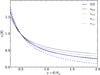 |
Fig. 1 The isothermal density profile (thick curve), and several of the transformed profiles κλ(θ), with λ ranging from 0.8 (flattest curve) to 1.2 (steepest curve), plotted as a function of x = θ/θE. Note that, if the SIS density profile provides a good fit to the lensing data, an equally good fit is obtained by all the κλ. |
3. Power-law mass profiles
The surveys just mentioned have demonstrated that the mean slope of the three-dimensional density profile of early-type lens galaxies, measured between the effective radius and the Einstein radius, is nearly isothermal, i.e. γ′ ~ 2, with relatively small variations (~±0.2) between different lenses. It must be pointed out that the slope of the density profile determined by this method is an average one, over the radial range between the effective radius and the Einstein radius; it does not imply that the density profile is indeed accurately described by a power law. In fact, from our understanding of the physical properties of galaxies, one would not expect the density profile in the central kiloparsecs region where the lensing effects occur to be a perfect power law (e.g. van de Ven et al. 2009; Cappellari et al. 2013, but see also Remus et al. 2013). These aforementioned surveys have concluded that about half of the mass inside the Einstein radius is contributed by baryonic material, the other half by dark matter (somewhat dependent on the assumed initial mass function, and thus the mass-to-light ratio, of the stellar population). Neither the luminous matter, nor the dark matter, individually are expected to follow an isothermal profile: the light (and baryonic mass) distribution in early-type galaxies is well described by a Sérsic profile, whereas dark matter-only numerical simulations suggest the dark matter in halos to have a “universal” profile, with an inner slope close to γ′ ~ 1 (Navarro et al. 1996). The dark matter density profile of real galaxies probably deviates from this universal profile, due to feedback processes and the contraction of the dark matter halo through the condensation of baryons due to cooling in the inner part. In any case, the fact that the observed mean slope is close to isothermal is most likely a conspiracy and does not imply that the power-law assumption can be extrapolated to radii smaller (or larger) than the Einstein radius (van de Ven et al. 2009).
Nevertheless, it has been common practice to model the radial mass profiles of lenses by a power law (e.g. Rusin et al. 2003; Suyu et al. 2010, 2013a). It must be pointed out that this assumption formally breaks the MSD, since the transformation of a power law of κ according to (1) is not a power law. In other words, the assumption of a power law picks out one member of the family (1) of mass models. Acknowledging the fact that we have no a priori reason to suspect κ to be a true power law, this formal breaking of the MSD may lead to biased results.
On the other hand, whereas a mass-sheet transformed power law is no longer a power law, it is approximately so, as long as λ is not very different from unity. For a power-law mass distribution, one finds that  (2)If we now denote with θmin and θmax the inner and outer radial coordinate of the region where strong lensing constraints are available, the ratio
  (3)is a measure of the deviation from a power law, with ξ = 1 for an exact power law.
We consider an isothermal model as reference, with κ(θ) = θE/(2θ), where θE is the Einstein angle of the lens. In Fig.1 we plot the density profile of a singular isothermal sphere (SIS), and several of the κλ(θ) obtained from (1). We see that over the radius range plotted, the transformed profiles appear almost as power laws, with a slope depending on λ. We quantify the slope in two different ways: first, by taking the local slope  (4)at the Einstein radius, yielding s = λ/(2 − λ). Second, we take the mean slope over the angular range θmin ≤ θ ≤ θmax,
 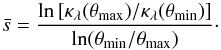 (5)For an SIS lens, the image positions are separated by 2θE; hence, if the positive parity image is found at θ = x θE, with 1 < x < 2, the negative parity image is located on the other side of the lens center, with | θ | = (2 − x)θE. Thus we choose θmin = (2 − x)θE, θmax = xθE.
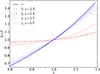 |
Fig. 2 For the mass models obtained by the transformation (1) of an SIS model, we plot the local slope s = λ/(2 − λ) at the Einstein radius as thick blue solid curve. The dashed and dotted thin blue curves show the mean slope |
In Fig.2, we have plotted the local slope s at the Einstein radius (solid blue curve), and the mean slope over the intervals 0.3 ≤ θ/θE ≤ 1.7 (dotted) and 0.5 ≤ θ/θE ≤ 1.5 (dashed) as thin blue curves, as a function of λ. Furthermore, we plot the parameter ξ (see Eq.(3)) over the same intervals as thick red curves. We see that ξ stays close to unity over a fairly wide range of λ, i.e., deviations from a power law are small over the intervals probed. This can also be seen by the fact that the mean slope  is very similar to the local slope s. Hence, a mass-sheet transformed power law remains a power law, to a good approximation (ξ deviates from 1 by less than 5% for λ ∈ [0.8,1.1] for the case x = 1.5), over the radius range typically probed by strong lensing, for quite a range of λ-values.
4. A composite model
In the previous section, we have studied the MST of a power law. Here, we present analytical and numerical experiments showing that the astrometry and photometry of synthetic lensed systems resulting from the lensing by the sum of two different density profiles can be reproduced with a single power law profile. We show that this degeneracy between profiles is coincidentally very similar to the effect of a MST and impacts only the time delay.
We start in Sect. 4.1 with a toy model which provides a simplistic analytic illustration of the freedom one has in choosing the mass models for a circular lens potential. In Sect. 4.2, we investigate numerically the situation for a more realistic non-circularly symmetric lens, and a complex and structured source composed of 10 compact structures leading to more than 20 lensed images (doubles or quadruples).
4.1. Toy data set
We follow Suyu (2012) who considered the possibility to constrain the slope of lenses in the case of a two-image system.
Hence, we assume to have a source consisting of two closely spaced components. For simplicity, we consider axi-symmetric mass distributions. We furthermore assume that the lensing properties are such that the images of the source components are located at θ1 and θ1 + Δθ on one side of the lensing galaxy, and at θ2 and θ2 − Δθ on the other side of the lens center, with θ1 > θ2 > 0. Hence, the separation of the two subcomponents is the same in both images. This implies that, when we try to model this image system with a power-law mass distribution, its slope will be isothermal. The Einstein radius of the SIS is θE = (θ1 + θ2)/2.
The same data can also be fit with a composite model, consisting of a Sérsic profile plus a power law, which should resemble a toy model of the mass distribution of baryons and the local distribution of dark matter in the inner part of the galaxy, respectively. Further specializing the Sérsic profile to an exponential, we write 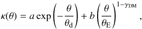 (6)where θd is the scale radius of the exponential. For a given choice of θd and 3D-slope γDM, one can find the values of the amplitudes a and b which satisfy the two constraints from the lensing information, i.e., which yield the same source positions for the two multiply imaged source components. Hence, this mass model can yield an exact solution of the lens equation. The corresponding algebra does not yield useful insight and will not be reproduced here.
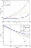 |
Fig. 3 Upper panel: the quantity ξ (blue solid curve), the mean slope |
As an example, we choose θ1 = 3θ2, and Δθ = θE/50. Furthermore, we set θd = 0.2θE and γDM = 1.75, yielding a ≈ 5.17 and b ≈ 0.36. The corresponding mass profile is shown as dashed black curve in the bottom panel of Fig.3; compared to the SIS model (shown in the same panel as thin solid curve), it is slightly steeper within the strong lensing region. The corresponding time delay is about 15% higher than for the SIS model, as expected from the steeper slope.
Next, we consider mass-sheet transformed versions of the profile described in (6). In the top panel of Fig.3, we show the parameter ξ defined in (3), evaluated between the radii x1 ≡ θ/θE = 0.5 and x2 = 1.5, i.e., over the region where strong lensing constraints are available, as a function of λ (blue solid curve). Over most of the parameter range plotted in the figure, | ξ − 1 | ≲ 0.1, i.e., in the radial range probed by strong lensing, the mass distribution fairly closely resembles a power law. The mean slope of the mass profile between these two radii is shown as dashed black curve; increasing λ yields steeper slopes, as expected. The red dotted curve shows the ratio of the time delay of the composite model, compared to that of the SIS; this ratio is a linear function of λ, as expected from the MST.
In the bottom panel of Fig.3, the resulting mass profiles κλ are shown for λ = 0.8 (blue solid curve), the original one κ1 ≡ κ (black dashed curve) and for λ = 1.19 (red dotted curve), the value of λ for which ξ ≈ 1, i.e., where the resulting mass profile is closest to a power law in the strong lensing region. Hence we see that the same strong lensing data can be fit with two different power laws, one global one with isothermal slope, and one which is locally almost exactly a power law, but with very different slope (and a resulting 37% larger value of τ = H0 Δt).
We conclude from this very simple example that there is a large freedom of fitting strong lensing data, not only due to the MSD, but also to our lack of well-motivated shapes of the total mass distribution of galaxies. Of course, this simple example may not be very realistic; in particular, we have not studied whether this model is able to satisfy any stellar kinematic constraints obtained from spectroscopy of the lens galaxy. We expect that such a more detailed study would yield constraints on the parameters θd and γDM in our model. However, the main conclusion – a substantial freedom in the choice of possible mass profiles for fitting lensing data – will be unchanged.
The profiles shown in the bottom panel of Fig.3 show a substantially different behavior for larger radii, compared to the SIS, and may appear unphysical. This is due to the simplified model of the dark matter profile as a global power law. However, as we will discuss is Sect. 5, this behavior at large radii is of no particular concern.
4.2. A complex lens system
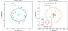 |
Fig. 4 Example of a complex lensed image system obtained from lensing by a composite mass distribution (Hernquist+gNFW) and well reproduced with a power-law mass distribution. Left: lensed image positions and critical curves for the fiducial composite model (light cyan) and for the power-law model (black). Right: corresponding caustics and source positions for the fiducial composite model (light orange) and for the power-law model (red). The small inset panel provides a zoom of the inner caustic. |
Our toy data set indicates that degeneracies between lens models could be a serious limitation to accurate lensing analysis. This model, however, provides a highly simplified view of a lens system. Real lens systems show more complex image configurations that need to be fitted with mass models, within the observational accuracy of positions. We now routinely measure lensed image positions to a few milli-arcsec accuracy and observe Einstein ring-like features1. It has been shown that those observational constraints were crucial to disentangle lens models (e.g. Kochanek et al. 2001; Cohn et al. 2001; Wucknitz et al. 2004; Suyu & Blandford 2006; Sluse et al. 2008, 2012; Suyu & Halkola 2010; Oguri et al. 2013) and we may think that this is sufficient to break the degeneracy outlined in the previous section (except, of course, the MSD). In order to investigate this question, we have simulated various ensembles of arbitrarily complex sources composed of 10 point-like features paving the source plane, and lensed them with a plausible lensing galaxy. We have then used power-law density profiles to fit the positions of the mock lensed images, and compared the retrieved flux ratios and time delays with the simulated ones.
A plausible model for a lensing galaxy has to include at least one component for the baryons and one for the dark matter halo. Following Courbin et al. (2011) in their study of the lensed system HE0435–1223, we have decided to model the stellar component with a Hernquist mass distribution and the dark matter halo with a generalized NFW profile. The density profile of the Hernquist (1990) profile is expressed as 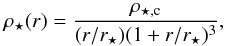 (7)where ρ⋆ ,c is a characteristic density and r⋆ the scale radius of the profile. The generalized NFW profile (Navarro et al. 1996) is
 ![\begin{equation} \rho_{h}(r) = \frac{\rho_{\rm h,\rm c}} {(r/r_{\rm s})^{\gamma_{\rm DM}} [1+(r/r_{\rm s})^2]^{(3-\gamma_{\rm DM})/2}}, \end{equation}](/articles/aa/full_html/2013/11/aa21882-13/aa21882-13-eq101.png) (8)where rs is the scale radius, γDM the inner slope of the density profile and ρh,c is a characteristic density.
(8)where rs is the scale radius, γDM the inner slope of the density profile and ρh,c is a characteristic density.
This particular choice of the mass distribution for the composite lens is to some extent arbitrary, but is sufficient for our aims. Courbin et al. (2011) generated an ensemble of galaxies which were dynamically stable, and had a stellar velocity dispersion compatible with the one observed in HE0435–1223. We used a subsample of those galaxies to create a set of about 1000 mock lensing galaxies. For simplicity, we kept the mass distribution spherically symmetric, and added an external shear (γ,θγ) = (0.1,90°). The Einstein radius was kept fixed at θE = 1.′′25 ± 0.′′05. We also fixed the scale radii of the two mass components at θs = rs/Dd ~ 4 θE, θ⋆ = r⋆/Dd ~ 0.8 θE; the two remaining free parameters of the model are then the ratio of the normalization of the two mass components and the inner dark matter slope γDM.
For each lens model, we have randomly generated 10 point-like components distributed in the source plane with a uniform probability distribution between the lens center β = 0 and βmax. We have calculated the positions of the lensed images using the public lens modeling code lensmodel (v1.99) developed by Keeton (2001), and assigned them an uncertainty of 0.004 arcsec on the position of each lensed image, representative of the best existing observational constraints. A better astrometric accuracy is sometimes achieved for radio or optical data of a few compact lensed images, but those positions often reveal astrometric perturbations produced by substructures close in projection to the lensed images and not accounted for by the smooth lens models. Those synthetic lensed images should also be equivalent to the constraints provided by a smooth extended image, such as an Einstein ring observed with the Hubble Space Telescope. Those synthetic data are then fitted with a power-law mass distribution 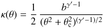 (9)plus external shear, where b is a normalization factor, θc is the core radius of the profile (assumed to be arbitrarily small, unless otherwise stated) and γ′ is the logarithmic slope of the 3D density profile [i.e. κ(θ) → θ1 − γ′ and ρ(θ) → θ− γ′], with γ′ = 2 for an isothermal profile.
We found that the power-law mass distribution could in general reproduce the mock lensed images extremely well (i.e. with a reduced χ2 ≤ 1). We show in Fig. 4 one particular example for which the lensed images generated with the composite model are perfectly reproduced with an almost isothermal lens. We clearly see that the two models have a nearly identical outer (tangential) critical curve. The inner critical curves are more different, but this does not come as a surprise since our power-law model was chosen to be nearly singular while our composite model has a relatively flat core. We discuss this effect hereafter.
Because the ability to fit a power-law model to the simulated lensed images did not depend on the parameters explored by our composite model (i.e. variable baryonic fraction fb and γDM), we focus on the fiducial example presented in Fig. 4 in the following. The fiducial model has an average projected baryon fraction ⟨fb( < θE)⟩ ~ 0.4, and γDM = 1.96. The lensed images generated with this model are fitted by a power law model with γ′ ~ 1.98. The approximate isothermality of the fitted power law model is not a generic result. For our ensemble of mock lenses, the fitted logarithmic slope of the power law was found in the range γ′ ∈ [1.55, 2.01]. The observed trend to fit model shallower than isothermal is likely incidental and is related to our particular choice of rs and r⋆. As we show hereafter, the slope of the fitted power law depends on the surface density close to the galaxy center.
The projected density profiles of the fiducial lens and of the fitted power-law profile are shown in Fig. 5. The slope and the surface density of the two models are very different. However, both models reproduce the same set of 26 lensed images (Fig. 4). Comparing the source morphology found for the fiducial and the power-law model, we see that the latter is simply a scaled-down version of the one found for the fiducial model, a behavior similar to what would be obtained with a mass-sheet transformation. In fact, the fitted power-law model (PL) is, to a good approximation, a mass-sheet transformed version of the fiducial model (fid), with source positions βPL = βfid/λ, and magnifications μPL ~ λ2 μfid, with λ ~ 1.19. For a MST, the time delays are also scaled as τPL ~ τfid/λ. This scaling of the time delays is verified in our fiducial case but not for the ensemble of mock lenses. The simple scaling of the source positions and magnifications implies that having a source which is extended instead of composed of many point-like structures would not help to break the degeneracy: the power-law and the fiducial model will lens two sources linearly scaled by a factor λ into an almost identical Einstein ring.
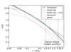 |
Fig. 5 Surface mass density of our fiducial model composed of a Hernquist (dashed red) + generalized NFW (dotted black) model. Two power-law models which reproduce equally well an ensemble of lensed images whose positions range typically in x ∈ [0.5,1.5] (vertical dashed lines) are shown. The solid blue curve is for a singular power-law model, whereas the green curve is for a power law with a core (see Sect. 4.2). |
In order to investigate whether some particular source configurations could break the degeneracy, we have generated 20 new sets of complex sources and lensed them with our fiducial model. Figure 6 displays the logarithmic slope of the fitted power law as a function of the position of the innermost lensed image xmin and colored based on the value of the χ2. We see that the power-law model provides an excellent representation of the mock data over a large range of image positions. However, the slope of the fitted power law decreases by a few percents with the increase of the width of the annulus containing the lensed images. Interestingly, the power-law model fits less accurately the mock data when images at a radius  are observed. For our fiducial model, this happened when
  . Figure 4 indicates that this situation occurs because the singular power-law model does not reproduce the inner critical curve.
In order to better match the inner critical curve, we have fitted the lensed images using a power-law model with a freely varying core θc (see Eq.(9)). We generated 80 different sets of sources with 10 components each to produce images very close/far from the center of the galaxy. This model allows us to obtain a nearly perfect fit (χ2 < 0.5) of all the 80 images configurations (down to xmin ~ 0.2). The power law retrieved with that model has a relatively large core radius (θc ~ 0.′′13) and a steeper density profile (γ′ ~ 2.3) which reproduces almost perfectly the one of the fiducial model between 0.15 < x < 0.7 (Fig. 5). Like in the case of the singular power law, the fitted value of γ′ depends on the range over which lensed images are observed. Again, the sources obtained with the two models (PL and fiducial) are almost identical up to an isotropic scaling factor λ. The time delay ratios are, however, not conserved perfectly between the two models, with deviations reaching several tens of percents for some image pairs. This shows that the transformation between the two lens models is not simply a MST.
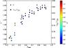 |
Fig. 6 Result of the fit of the (singular) power-law model to the composite model for 20 different sets of complex sources. For each realization of the complex source, we show the value of the logarithmic slope γ′ (circles) of the fitted power law as a function of the position of the inner-most lensed image in the system (xmin). The time-delay ratio is also shown (star-like symbols). The color code shows the (non-reduced) χ2 obtained for the fit of the power-law model; the typical number of degrees of freedom is ~30. |
We can now ask the question whether the power law models are also compatible with the velocity dispersion of the lens. The composite model we used has a velocity dispersion σ = 261 km s-1, as measured within a 1′′ slit. Following the combined lensing+virial formalism introduced by Agnello et al. (2013), we have estimated that the luminosity-weighted line of sight velocity dispersion of the power-law model, measured within a 1′′ aperture, is σlos,L(R < 1′′) = 262 km s-1, in perfect agreement with the value found for the fiducial model. The velocity dispersion of the power law with a finite core, characterized by γ′ = 2.3, is more difficult to assess. Following the same prescription as above, we find σlos,L(R < 1′′) = 375 km s-1. However, this estimate does not account for the presence of a finite core in the center of the profile. To estimate the impact of the core, we use the results of Keeton & Kochanek (1998; see also Dutton et al. 2011), to derive the circular velocity of an isothermal profile in the presence of a core. Following that formalism, we find for a core radius of θc = 0.′′13 that the circular velocity is reduced by ~30% at a radius of half the slit width (i.e. 0.′′5). Assuming that this scaling of the circular velocity is also valid for non-isothermal profiles, and knowing that the velocity dispersion is proportional to the circular velocity (Padmanabhan et al. 2004; Cappellari et al. 2013), we calculate the velocity dispersion of the power law model with a core, σlos,L(R < 1′′) = 288 km s-1. Hence, the power-law models which are degenerate with our composite fiducial model also have a velocity dispersion compatible with that one if velocity dispersion uncertainties in agreement with typical observations (i.e. about 10%) are assumed. We may be careful in generalizing this result too much, since our fiducial composite model and power-law models are not universal representations of the density profile of lensing galaxies. The velocity dispersion will always reduce the family of degenerate models reproducing the data, but our illustrative example shows that models predicting very different time delays can be found.
The above examples show that even for a non-circular lens potential there is significant freedom in choosing the lens model, even in presence of a velocity dispersion measurement. This freedom is due to the fact that our composite mass model transforms into an approximate local power law by means of a mass sheet-like transformation. It is important to realize that this transformation is formally unrelated to the external convergence from the environment (which we discuss in the next section). It exists because of the freedom one has in modifying the gravitational potential in regions not probed by the lensed images (i.e. for x < xmin and x > xmax). The freedom we have is however limited because the mass interior to the Einstein radius cannot change between the two models. A measurement of the time delays between lensed images, assuming a value of H0 determined by other methods, can break this degeneracy since τ is mostly sensitive to the slope of the mass profile near the Einstein radius (Gorenstein et al. 1988; Kochanek 2002). The observation of a second source at a different redshift should also break that degeneracy. Indeed, in case of multiple sources, a set of equations similar to (1) has to be valid for each different source redshift, hence different distance ratios Dds/Ds. As explained in details in Saha (2000, Sect. 2.2), Bradač et al. (2004), or Liesenborgs & De Rijcke (2012, Sect. 4), this effectively breaks the MSD. This implies that strong lensing studies by galaxy clusters, where sources at multiple redshifts are commonly observed, should be less impacted by that degeneracy. However, compact substructures in the potential, producing monopole-like degeneracies, may be a concern (Liesenborgs et al. 2009; Liesenborgs & De Rijcke 2012). For galaxy-scale lenses, sources at multiple redshifts are rarely observed, but a few systems with double Einstein rings are known2 (Eigenbrod et al. 2006; Gavazzi et al. 2008). We can also naively think that the observation of a central image would be of great relevance to break the degeneracy, but the magnification of the latter image constrains only the very inner core of the lensing galaxy and may be unrelated to the global shape of the mass distribution.
After the first version of this paper was published on the arXiv, Suyu et al. (2013b) modeled the time-delay lens system J1131−1231 with a composite model, using the observed light profile of the lens to fix the baryonic component, and a standard NFW-profile for the dark matter. This model yielded a value for τ which is good agreement with their earlier analysis based on a power-law mass model. This result shows that the same data can be reproduced with more than one class of models. However, over the radial range where lensing data are available, the mass profile of the composite lens and the best-fitting power-law model essentially coincide. Therefore, the new model does not probe the freedom of the lens model offered by the MST. It is possible that this agreement is a coincidence, originating from the specific shape of the luminosity profile and the choice of an inner slope of the dark matter profile of − 1. As mentioned before, this slope is obtained from dark matter-only simulations, but is most likely altered once baryon cooling comes into play (see, e.g., Scannapieco et al. 2012, and references therein).
5. The external convergence
The original motivation for Falco et al. (1985) to consider the MSD was related to the first gravitational lens system 0957+561, where the main lens is embedded in a group or low-mass cluster of galaxies. The unexpectedly large angular separation of ~ 6″ in this system hinted at a substantial influence of the mass distribution of the cluster on the lensing properties of the lens. Neglecting shear, the prime effect of the cluster is to yield an additional surface mass density at the location of the main lens galaxy, which boosts the angular splitting. Falco et al. pointed out that there is a trade-off between the mass parameters of the main lensing galaxy and the amplitude of this external convergence, which is described by the MST (1). This physical interpretation yielded the name of the transformation.
Based on that, one frequently finds the MST written in the form  (10)which obviously is fully equivalent to (1). However, the way (10) is written suggests a physical interpretation of the MST: if the original mass profile κ(θ) is chosen such that κ → 0 as | θ | → ∞, then the parameter κext is interpreted as the convergence far from the lens (e.g., the convergence contributed by a large-scale matter inhomogeneity in the direction of the main lens, such as a cluster in which the lens is embedded). In this case, one may investigate the line-of-sight to the lens to find indications for an over- (or under)density of galaxies, which can then be used as a proxy for the corresponding κext. In contrast, in its form (1) the transformation is of purely mathematical nature, without any interpretation of λ.
We believe that the interpretation of (10) is misleading. Suppose some mass distribution κ(θ) provides a good model fit to the lensing data, and suppose that this analytical model (such as an isothermal ellipse) is chosen as to vanish for large radii. Then for any λ ≠ 1, the asymptotic value of κλ(θ) for large separations is 1 − λ, i.e., in general different from zero. However, this does not imply that the lens is embedded in an external convergence with κext = 1 − λ: the strongly lensed images are located close to the center of the lens, typically within two Einstein radii, i.e., in regions where κ ≳ 0.3. Assuming elliptical symmetry, the mass profile outside this region does not affect the lensing properties, and is therefore not constrained. We note however that in case of non-elliptical symmetry, due to a gradient of convergence produced by nearby companion galaxies, or a group or cluster, lensing observables will be affected. There are many examples where this happens, including many time-delay lenses.
Assuming then that the analytic profile κ(θ) is a good description of the global mass profile, just because it provides a good fit to the lensing constraints, is a strong extrapolation, given that we have no good physical model for the density profile of galaxies – as mentioned before, we do not understand why the sum of the baryonic density and the dark matter distribution superpose to an almost isothermal profile at radii close to the Einstein radius.
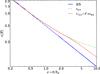 |
Fig. 7 The solid blue curve shows the isothermal density profile, the dashed curve shows the mass-sheet transformed profile κλ with λ = 0.9, and the thin solid red curve shows κ0., modified by multiplication with a smooth function F as described in the text. |
Mathematically, we can define a function F(θ) which is unity for | θ | ≲ 2θE, and then decreases smoothly to zero for larger radii. Then,  is unchanged in the inner regions of the lens (provided F shares the same symmetries as κ, e.g., being constant on confocal ellipses) and decreases to 0 at large separation | θ |, with no relation to an external convergence. Conversely, we can slightly redefine F such that
  decreases to any desired value of κext for large radii. Figure7 illustrates this with a simple example for such a transformation. Hence, studying the environment of a lens may be of limited use for breaking the MSD.
6. Conclusions
The mass-sheet degeneracy is the largest obstacle in gravitational lensing to obtain model-independent accurate quantitative results. Apart from the mass inside the Einstein radius, the masses inside all other radii are affected by the MSD, as is the (slope of the) radial mass profile. One instructive example of that statement can be found in Fig. 5 of Coe et al. (2012), where different methods for obtaining the density profile in the inner region of the lensing cluster Abell 2261 were employed; the resulting mass profiles are quite different, despite the fact that several strong lensing systems are identified in this cluster. For most galaxy-scale lenses, the observational situation is often worse, with only one source being multiply imaged in general.
The MST affects the product H0 Δt of the Hubble constant and the time delay, and hence the determination of H0 from lens systems. In this paper, we have pointed out a number of issues related to mass models and the MSD; in particular, we question the commonly made assumption that the density profile is a global power law, an assumption which implicitly breaks the MSD. Given our lack of understanding of the conspiracy that yields a mean slope close to an isothermal profile from a superposition of a Sérsic profile, which describes the luminous matter in galaxies, and that of the dark matter profile, we believe that it is timely to investigate the impact of the single power-law assumption on lensing results. This is particularly true close to the region of strong lensing features, where the observed fraction of dark matter is about one half, i.e., most likely the transition region from baryon-dominance to dark matter-dominance in lens galaxies. Using plausible lens models, we have shown that composite models made of a Sérsic (or Hernquist)+dark matter profile could be transformed through a MST-like transformation into a mass distribution close to power law over the range of radii constrained by lensed images. This probably explains why galaxy-lensing data may generally be well fitted with power law mass distributions despite the more complex intrinsic mass distribution of the lens. On the other hand, the MST (1) transforms a power law into a profile which resembles to good approximation a power law, but not an exact one. Preference of an exact power law therefore seems to some degree arbitrary.
We also question the physical interpretation of the MST to be directly related to an external convergence, since this implies a extrapolation of the density profile well beyond the region where the mass profile is constrained by lensing information. Again, due to the lack of accurate physical models for the density distribution in galaxies, such an extrapolation may not be appropriate. In particular, the frequently employed isothermal profile must break down at large radii, since the dark matter profile is steeper than isothermal for large r, and also because the total mass diverges linearly.
Together, we therefore question whether the determination of the Hubble constant from gravitational lensing indeed is as accurate as sometimes claimed in the literature. Whereas the freedom offered by the MST (1) cannot be stretched arbitrarily – values of λ too different from unity may indeed lead to unphysical mass profiles, and in particular violate constraints from the measured stellar velocity dispersion of the lens galaxy, some ~ 10% deviations (or even larger) of λ from unity seem quite plausible. The Hubble constant as determined with free-form lens modeling (e.g. Saha et al. 2006; Coles 2008; Paraficz & Hjorth 2010) may be less prone to the MSD because free-form lens models naturally explore a large variety of mass distributions. Enlarging the parameter space may, however, not guarantee an unbiased estimate of H0. Indeed, despite some priors on the variation of the potential with radius (Saha & Williams 2004), there is no security that unphysical mass distributions (e.g. dynamically unstable) are not part of the ensemble of valid lens models. The consistency between H0 as derived with pixelated mass models and the value published by Planck indicates that the current method works reasonably well, but we think that breaking the MSD with free-form lens models is not yet enough controlled to derive an accurate value of H0.
Whatever the lens modeling approach, the impact of the MST on the value of H0 from gravitational lensing has to be quantified carefully. This is particularly true because the resulting effect on H0 may not be statistical, and thus not average out when considering samples of lens systems. If the true mass profile in the strong lensing region of galaxies is systematically curved (say convex, in the transition region between baryon dominance and dark matter dominance), the power-law assumption will yield a systematic bias on the estimates of H0. This is because the sign of (1 − λ) determines the sign of curvature a mass-sheet transformed power-law model will attain. Fadely et al. (2010), in their in-depth analysis of the lens system Q0957+561 using two-component mass models and constraints from weak lensing, have investigated how their estimate of H0 was limited by the MSD.
On the other hand, a better understanding of galaxy formation and the physics of galaxies may allow one to reduce the freedom in lens models. The apparent conspiracy for lensing galaxies to show profiles close to isothermal around one Einstein radius, or even at larger radii (e.g. Gavazzi et al. 2007; Koopmans et al. 2009; van de Ven et al. 2009; Humphrey & Buote 2010; Dutton & Treu 2013), could be an indication that the systematic errors introduced by the choice of an isothermal model are small or could be quantified based on some observational properties of the galaxies. The study of mock lens galaxies based on parametrized density distributions (van de Ven et al. 2009) or hydrodynamical simulations may enable one to estimate quantitatively how large this effect is on real galaxies, and to see whether systematic errors introduced by the use of a particular type of lens models cannot be calibrated.
From the above discussion, it is also clear that if accurate measurements of the Hubble constant are obtained with an independent method, lenses with measured time delays are the best suited ones to probe the density slope in the inner part of galaxies (Read et al. 2007; Fadely et al. 2010). The modeling of such systems may enable one to investigate deviations from simple power-law profiles, and, together with a determination of the baryonic mass from the observed light profile of the lens galaxy and its velocity dispersion, to learn about the shape of the dark matter profile in the inner region of galaxy halos. This indeed makes time delay lenses a unique tool for studying the inner parts of dark matter halos in galaxies.
The double-source nature of the lens SDSSJ0924+0219 reported in Eigenbrod et al. (2006) is more speculative than for the system SDSSJ0946+1006 – also known as the “Jackpot” – discovered by Gavazzi et al. (2008) and further studied by Sonnenfeld et al. (2012).
Acknowledgments
We thank Sherry Suyu for numerous and sometimes controversial discussions which have inspired this work. Olaf Wucknitz, Yves Revaz, Chris Kochanek, Andrea Macciò are also acknowledged for useful discussions. We thank the anonymous referee for his thoughtful comments on the manuscript. Part of this work was supported by the German Deutsche Forschungsgemeinschaft, DFG project number SL172/1-1.
References
- Agnello, A., Auger, M. W., & Evans, N. W. 2013, MNRAS, 429, L35 [NASA ADS] [Google Scholar]
- Auger, M. W., Treu, T., Bolton, A. S., et al. 2010, ApJ, 724, 511 [NASA ADS] [CrossRef] [Google Scholar]
- Barnabé, M., & Koopmans, L. V. E. 2007, ApJ, 666, 726 [NASA ADS] [CrossRef] [Google Scholar]
- Barnabé, M., Czoske, O., Koopmans, L., et al. 2009, MNRAS, 399, 21 [NASA ADS] [CrossRef] [Google Scholar]
- Barnabé, M., Czoske, O., Koopmans, L. V. E., Treu, T., & Bolton, A. S. 2011, MNRAS, 415, 2215 [NASA ADS] [CrossRef] [Google Scholar]
- Bauer, A. H., Baltay, C., Ellman, N., et al. 2012, ApJ, 749, 56 [NASA ADS] [CrossRef] [Google Scholar]
- Bradač, M., Lombardi, M., & Schneider, P. 2004, A&A, 424, 13 [NASA ADS] [CrossRef] [EDP Sciences] [Google Scholar]
- Cappellari, M., Scott, N., Alatalo, K., et al. 2013, MNRAS, 432, 1709 [NASA ADS] [CrossRef] [Google Scholar]
- Coe, D., Umetsu, K., Zitrin, A., et al. 2012, ApJ, 757, 22 [NASA ADS] [CrossRef] [Google Scholar]
- Cohn, J. D., Kochanek, C. S., McLeod, B. A., & Keeton, C. R. 2001, ApJ, 554, 1216 [NASA ADS] [CrossRef] [Google Scholar]
- Coles, J. 2008, ApJ, 679, 17 [NASA ADS] [CrossRef] [Google Scholar]
- Courbin, F., Chantry, V., Revaz, Y., et al. 2011, A&A, 536, A53 [NASA ADS] [CrossRef] [EDP Sciences] [Google Scholar]
- Dutton, A. A., & Treu, T. 2013, MNRAS, submitted [arXiv:1303.4389] [Google Scholar]
- Dutton, A. A., Brewer, B. J., Marshall, P. J., et al. 2011, MNRAS, 417, 1621 [NASA ADS] [CrossRef] [Google Scholar]
- Eigenbrod, A., Courbin, F., Dye, S., et al. 2006, A&A, 451, 747 [NASA ADS] [CrossRef] [EDP Sciences] [Google Scholar]
- Eulaers, E., & Magain, P. 2011, A&A, 536, A44 [NASA ADS] [CrossRef] [EDP Sciences] [Google Scholar]
- Eulaers, E., Tewes, M., Magain, P., et al. 2013, A&A, 553, A121 [NASA ADS] [CrossRef] [EDP Sciences] [Google Scholar]
- Fadely, R., Keeton, C. R., Nakajima, R., & Bernstein, G. M. 2010, ApJ, 711, 246 [NASA ADS] [CrossRef] [Google Scholar]
- Falco, E. E., Gorenstein, M. V., & Shapiro, I. I. 1985, ApJ, 289, L1 [Google Scholar]
- Fohlmeister, J., Kochanek, C. S., Falco, E. E., et al. 2013, ApJ, 764, 186 [NASA ADS] [CrossRef] [Google Scholar]
- Gavazzi, R., Treu, T., Rhodes, J. D., et al. 2007, ApJ, 667, 176 [NASA ADS] [CrossRef] [Google Scholar]
- Gavazzi, R., Treu, T., Koopmans, L. V. E., et al. 2008, ApJ, 677, 1046 [NASA ADS] [CrossRef] [Google Scholar]
- Gorenstein, M. V., Shapiro, I. I., & Falco, E. E. 1988, ApJ, 327, 693 [NASA ADS] [CrossRef] [Google Scholar]
- Grogin, N. A., & Narayan, R. 1996, ApJ, 464, 92 [NASA ADS] [CrossRef] [Google Scholar]
- Hernquist, L. 1990, ApJ, 356, 359 [NASA ADS] [CrossRef] [Google Scholar]
- Humphrey, P. J., & Buote, D. A. 2010, MNRAS, 403, 2143 [NASA ADS] [CrossRef] [Google Scholar]
- Keeton, C. R. 2001 [arXiv:astro-ph/0102340] [Google Scholar]
- Keeton, C. R., & Kochanek, C. S. 1998, ApJ, 495, 157 [NASA ADS] [CrossRef] [Google Scholar]
- Kochanek, C. S. 2002, ApJ, 578, 25 [NASA ADS] [CrossRef] [Google Scholar]
- Kochanek, C. S., Keeton, C. R., & McLeod, B. A. 2001, ApJ, 547, 50 [NASA ADS] [CrossRef] [Google Scholar]
- Kochanek, C. S., Schneider, P., & Wambsganss, J. 2004, Part 2 of Gravitational Lensing: Strong, Weak & Micro, Proc. 33rd Saas-Fee Advanced Course, eds. G. Meylan, P. Jetzer, & P. North (Berlin: Springer-Verlag) [Google Scholar]
- Koopmans, L. V. E. 2004 [arXiv:astro-ph/0412596] [Google Scholar]
- Koopmans, L. V. E., Bolton, A., Treu, T., et al. 2009, ApJ, 703, L51 [NASA ADS] [CrossRef] [Google Scholar]
- Kundic, T., Turner, E. L., Colley, W. N., et al. 1997, ApJ, 482, 75 [NASA ADS] [CrossRef] [Google Scholar]
- Liesenborgs, J., & De Rijcke, S. 2012, MNRAS, 425, 1772 [NASA ADS] [CrossRef] [Google Scholar]
- Liesenborgs, J., De Rijcke, S., Dejonghe, H., & Bekaert, P. 2009, MNRAS, 397, 341 [NASA ADS] [CrossRef] [Google Scholar]
- Navarro, J. F., Frenk, C. S., & White, S. D. M. 1996, ApJ, 462, 563 [NASA ADS] [CrossRef] [Google Scholar]
- Oguri, M., Schrabback, T., Jullo, E., et al. 2013, MNRAS, 429, 482 [NASA ADS] [CrossRef] [Google Scholar]
- Padmanabhan, N., Seljak, U., Strauss, M. A., et al. 2004, New A, 9, 329 [Google Scholar]
- Paraficz, D., & Hjorth, J. 2010, ApJ, 712, 1378 [NASA ADS] [CrossRef] [Google Scholar]
- Planck Collaboration 2013, A&A, submitted [arXiv:1303.5076] [Google Scholar]
- Read, J. I., Saha, P., & Macciò, A. V. 2007, ApJ, 667, 645 [NASA ADS] [CrossRef] [Google Scholar]
- Refsdal, S. 1964, MNRAS, 128, 307 [NASA ADS] [CrossRef] [Google Scholar]
- Refsdal, S., & Surdej, J. 1994, Rep. Prog. Phys., 57, 117 [NASA ADS] [CrossRef] [Google Scholar]
- Remus, R.-S., Burkert, A., Dolag, K., et al. 2013, ApJ, 766, 71 [NASA ADS] [CrossRef] [Google Scholar]
- Romanowsky, A. J., & Kochanek, C. S. 1999, ApJ, 516, 18 [NASA ADS] [CrossRef] [Google Scholar]
- Rusin, D., & Kochanek, C. S. 2005, ApJ, 623, 666 [NASA ADS] [CrossRef] [Google Scholar]
- Rusin, D., Kochanek, C. S., & Keeton, C. R. 2003, ApJ, 595, 29 [NASA ADS] [CrossRef] [Google Scholar]
- Saha, P. 2000, AJ, 120, 1654 [NASA ADS] [CrossRef] [Google Scholar]
- Saha, P., & Williams, L. L. R. 2004, AJ, 127, 2604 [NASA ADS] [CrossRef] [Google Scholar]
- Saha, P., Coles, J., Macciò, A. V., & Williams, L. L. R. 2006, ApJ, 650, L17 [NASA ADS] [CrossRef] [Google Scholar]
- Scannapieco, C., Wadepuhl, M., Parry, O. H., et al. 2012, MNRAS, 423, 1726 [Google Scholar]
- Schneider, P., & Seitz, C. 1995, A&A, 294, 411 [NASA ADS] [Google Scholar]
- Schneider, P., Ehlers, J., & Falco, E. E. 1992, Gravitational Lenses, XIV (Berlin, Heidelberg, New York: Springer-Verlag, Also Astronomy and Astrophysics Library) [Google Scholar]
- Sluse, D., Courbin, F., Eigenbrod, A., & Meylan, G. 2008, A&A, 492, L39 [NASA ADS] [CrossRef] [EDP Sciences] [Google Scholar]
- Sluse, D., Chantry, V., Magain, P., Courbin, F., & Meylan, G. 2012, A&A, 538, A99 [NASA ADS] [CrossRef] [EDP Sciences] [Google Scholar]
- Sonnenfeld, A., Treu, T., Gavazzi, R., et al. 2012, ApJ, 752, 163 [NASA ADS] [CrossRef] [Google Scholar]
- Suyu, S. H. 2012, MNRAS, 426, 868 [NASA ADS] [CrossRef] [Google Scholar]
- Suyu, S. H., & Blandford, R. D. 2006, MNRAS, 366, 39 [NASA ADS] [Google Scholar]
- Suyu, S. H., & Halkola, A. 2010, A&A, 524, A94 [NASA ADS] [CrossRef] [EDP Sciences] [Google Scholar]
- Suyu, S. H., Marshall, P. J., Auger, M. W., et al. 2010, ApJ, 711, 201 [NASA ADS] [CrossRef] [Google Scholar]
- Suyu, S. H., Auger, M. W., Hilbert, S., et al. 2013a, ApJ, 766, 70 [NASA ADS] [CrossRef] [Google Scholar]
- Suyu, S. H., Treu, T., Hilbert, S., et al. 2013b, ApJL, submitted [arXiv:1306.4732] [Google Scholar]
- Tewes, M., Courbin, F., Meylan, G., et al. 2013, A&A, 556, A22 [NASA ADS] [CrossRef] [EDP Sciences] [Google Scholar]
- Treu, T., & Koopmans, L. V. E. 2002, ApJ, 575, 87 [NASA ADS] [CrossRef] [Google Scholar]
- van de Ven, G., Mandelbaum, R., & Keeton, C. R. 2009, MNRAS, 398, 607 [NASA ADS] [CrossRef] [Google Scholar]
- Walsh, D., Carswell, R. F., & Weymann, R. J. 1979, Nature, 279, 381 [NASA ADS] [CrossRef] [PubMed] [Google Scholar]
- Witt, H. J., Mao, S., & Schechter, P. L. 1995, ApJ, 443, 18 [NASA ADS] [CrossRef] [Google Scholar]
- Witt, H. J., Mao, S., & Keeton, C. R. 2000, ApJ, 544, 98 [NASA ADS] [CrossRef] [Google Scholar]
- Wucknitz, O. 2002, MNRAS, 332, 951 [NASA ADS] [CrossRef] [Google Scholar]
- Wucknitz, O., Biggs, A. D., & Browne, I. W. A. 2004, MNRAS, 349, 14 [NASA ADS] [CrossRef] [Google Scholar]
All Figures
|
Fig. 1 The isothermal density profile (thick curve), and several of the transformed profiles κλ(θ), with λ ranging from 0.8 (flattest curve) to 1.2 (steepest curve), plotted as a function of x = θ/θE. Note that, if the SIS density profile provides a good fit to the lensing data, an equally good fit is obtained by all the κλ. |
| In the text | |
|
Fig. 2 For the mass models obtained by the transformation (1) of an SIS model, we plot the local slope s = λ/(2 − λ) at the Einstein radius as thick blue solid curve. The dashed and dotted thin blue curves show the mean slope |
| In the text | |
|
Fig. 3 Upper panel: the quantity ξ (blue solid curve), the mean slope |
| In the text | |
|
Fig. 4 Example of a complex lensed image system obtained from lensing by a composite mass distribution (Hernquist+gNFW) and well reproduced with a power-law mass distribution. Left: lensed image positions and critical curves for the fiducial composite model (light cyan) and for the power-law model (black). Right: corresponding caustics and source positions for the fiducial composite model (light orange) and for the power-law model (red). The small inset panel provides a zoom of the inner caustic. |
| In the text | |
|
Fig. 5 Surface mass density of our fiducial model composed of a Hernquist (dashed red) + generalized NFW (dotted black) model. Two power-law models which reproduce equally well an ensemble of lensed images whose positions range typically in x ∈ [0.5,1.5] (vertical dashed lines) are shown. The solid blue curve is for a singular power-law model, whereas the green curve is for a power law with a core (see Sect. 4.2). |
| In the text | |
|
Fig. 6 Result of the fit of the (singular) power-law model to the composite model for 20 different sets of complex sources. For each realization of the complex source, we show the value of the logarithmic slope γ′ (circles) of the fitted power law as a function of the position of the inner-most lensed image in the system (xmin). The time-delay ratio is also shown (star-like symbols). The color code shows the (non-reduced) χ2 obtained for the fit of the power-law model; the typical number of degrees of freedom is ~30. |
| In the text | |
|
Fig. 7 The solid blue curve shows the isothermal density profile, the dashed curve shows the mass-sheet transformed profile κλ with λ = 0.9, and the thin solid red curve shows κ0., modified by multiplication with a smooth function F as described in the text. |
| In the text | |
Current usage metrics show cumulative count of Article Views (full-text article views including HTML views, PDF and ePub downloads, according to the available data) and Abstracts Views on Vision4Press platform.
Data correspond to usage on the plateform after 2015. The current usage metrics is available 48-96 hours after online publication and is updated daily on week days.
Initial download of the metrics may take a while.